Article

Global Evapotranspiration Datasets Assessment Using Water Balance in South America

by
Anderson Ruhoff
1,*,
Bruno Comini de Andrade
1,
Leonardo Laipelt
1,
Ayan Santos Fleischmann
2,
Vinícius Alencar Siqueira
1,
Adriana Aparecida Moreira
1,
Rafael Barbedo
1,
Gabriele Leão Cyganski
1,
Gabriel Matte Rios Fernandez
1,
João Paulo Lyra Fialho Brêda
1,
Rodrigo Cauduro Dias de Paiva
1,
Adalberto Meller
3,
Alexandre de Amorim Teixeira
3,
Alexandre Abdalla Araújo
3,
Marcus André Fuckner
3 and
Trent Biggs
4
1
Instituto de Pesquisas Hidráulicas, Universidade Federal do Rio Grande do Sul, Porto Alegre 91501-970, RS, Brazil
2
Mamirauá Institute for Sustainable Development, Tefe 69553-225, AM, Brazil
3
Agência Nacional de Águas e Saneamento Básico (ANA), Brasilia 70610-200, DF, Brazil
4
Department of Geography, San Diego State University, San Diego, CA 92182, USA
*
Author to whom correspondence should be addressed.
Remote Sens. 2022, 14(11), 2526; https://doi.org/10.3390/rs14112526
Submission received: 1 April 2022 / Revised: 14 May 2022 / Accepted: 21 May 2022 / Published: 25 May 2022
(This article belongs to the Special Issue Remote Sensing of Land–Atmosphere Interactions)

Abstract

:
Evapotranspiration ( E T ) connects the land to the atmosphere, linking water, energy, and carbon cycles. E T is an essential climate variable with a fundamental importance, and accurate assessments of the spatiotemporal trends and variability in E T are needed from regional to continental scales. This study compared eight global actual E T datasets ( E T g l ) and the average actual E T ensemble ( E T e n s ) based on remote sensing, climate reanalysis, land-surface, and biophysical models to E T computed from basin-scale water balance ( E T w b ) in South America on monthly time scale. The 50 small-to-large basins covered major rivers and different biomes and climate types. We also examined the magnitude, seasonality, and interannual variability of E T , comparing E T g l and E T e n s with E T w b . Global E T datasets were evaluated between 2003 and 2014 from the following datasets: Breathing Earth System Simulator (BESS), ECMWF Reanalysis 5 (ERA5), Global Land Data Assimilation System (GLDAS), Global Land Evaporation Amsterdam Model (GLEAM), MOD16, Penman–Monteith–Leuning (PML), Operational Simplified Surface Energy Balance (SSEBop) and Terra Climate. By using E T w b as a basis for comparison, correlation coefficients ranged from 0.45 (SSEBop) to 0.60 ( E T e n s ), and RMSE ranged from 35.6 ( E T e n s ) to 40.5 mm·month−1 (MOD16). Overall, E T g l estimates ranged from 0 to 150 mm·month−1 in most basins in South America, while E T w b estimates showed maximum rates up to 250 mm·month−1. E T g l varied by hydroclimatic regions: (i) basins located in humid climates with low seasonality in precipitation, including the Amazon, Uruguay, and South Atlantic basins, yielded weak correlation coefficients between monthly E T g l and E T w b , and (ii) tropical and semiarid basins (areas where precipitation demonstrates a strong seasonality, as in the São Francisco, Northeast Atlantic, Paraná/Paraguay, and Tocantins basins) yielded moderate-to-strong correlation coefficients. An assessment of the interannual variability demonstrated a disagreement between E T g l and E T w b in the humid tropics (in the Amazon), with E T g l showing a wide range of interannual variability. However, in tropical, subtropical, and semiarid climates, including the Tocantins, São Francisco, Paraná, Paraguay, Uruguay, and Atlantic basins (Northeast, East, and South), we found a stronger agreement between E T g l and E T w b for interannual variability. Assessing E T datasets enables the understanding of land–atmosphere exchanges in South America, to improvement of E T estimation and monitoring for water management.

Graphical Abstract

1. Introduction

South America is a major source of water to the atmosphere, being responsible for 21.7% of global actual evapotranspiration ( E T ) from the continents [1]. It is also the home of important ecosystems with high productivity, such as the Amazon, with tight feedbacks among E T , land surface, and the atmosphere [2], with E T playing a direct role on vegetation development [3]. Recycled precipitation ( P ) through E T regulates the continent’s climate and water cycles [4]. Furthermore, South American countries are major world food providers, and cropland expansion—in association with land cover changes—has significantly altered the surface energy partition, and thus E T fluxes [5,6]. As an essential climate variable [7,8], monitoring E T is relevant for both supporting new water-infrastructure projects and for regulating water uses to avoid water conflicts, as well as to achieve the United Nations (UN) Sustainable Development Goals [9]. There is a need to estimate water fluxes in the context of national- to continental-scale water management, e.g., to fulfill the needs of Environmental and Economical Water Accounting frameworks [10,11]. Understanding fluxes at the land–atmosphere interface contributes to better estimation of land-boundary conditions in earth-surface models [12,13], consequently improving the accuracy of short- to long-term climate modeling [14]. Accurate estimates of E T may be also useful for the calibration of hydrological models [15,16], which ultimately lead to better prediction of anomalously wet and dry periods and increased confidence regarding climate-change projections.
Actual E T , the combined process of evaporation of water from the surface and transpiration from vegetation, is a major component of the land-energy and hydrological cycles. Currently, local E T measurements can be obtained through a wide range of techniques, including—but not limited to—Bowen ratio systems, weighing lysimeters, and eddy covariance flux towers [17]. Some initiatives, such as the FLUXNET network [18,19], for example, have developed standards for data collection and created a global eddy covariance dataset from regional networks. Yet, like in most parts of the world, South America faces a very sparse coverage of field E T observations. In addition, recent years have seen a boom of global datasets that allow mapping E T from regional to global scales, made possible due to an increasing computational capacity, combined with the launching of several satellite missions [20]. Information obtained through remote-sensing datasets, from visible-to-thermal infrared bands, can be used to retrieve land-surface temperature, vegetation phenology, and other surface properties [21], which in turn are used as inputs to algorithms specifically developed for estimating E T . Typical algorithms for this purpose are the surface energy balance (SEB) approaches [22,23,24], physical equations based on vegetation phenology and potential E T equations (e.g., Penman–Monteith and Priestley–Taylor) [25,26], statistical or machine-learning models [27,28], as well as water-balance methods [29,30,31]. In parallel, land-surface models (LSMs) simulate water and energy fluxes through physical and conceptual representations of the terrestrial hydrological system [32], with increasing focus on the depiction of biophysical and biogeochemical processes related to plant and carbon dynamics [33]. LSMs are able to provide global estimates of E T when forced with meteorological data produced in combination with atmospheric models, reanalysis, and data-assimilation techniques [34,35].
Despite the significant advances in remote sensing and LSM, the estimation of E T is challenging and subject to major uncertainties. For instance, thermal remote-sensing data required for the application of SEB models are only reliable for cloud-free conditions, and such methods are very sensitive to the estimation of surface and near-surface temperature [36]. E T models, in general, are dependent on the accuracy of surface net radiation, which usually explains up to 80% of the E T variability [37], while methods that use physical equations are also subject to errors in additional meteorological variables [36], as well as to estimation of surface and canopy resistance as in the case of the Penman–Monteith approach [38]. Similarly, substantial uncertainties in LSMs are attributed to the existence of a large number of parameters, errors in forcing data, and deficiencies in model structure [32,33].
The increasing availability of global datasets, with different degrees of accuracy, urges effective methods to understand their uncertainties in both spatial and temporal dimensions. While global-scale assessments of E T datasets have been frequently reported over the last decade [39,40,41,42], in South America it has been only recently conducted, but with a focus on specific biomes, such as the Amazon basin [43,44,45]. In particular, Sörensson and Ruscica [46] evaluated the similarity among nine global E T datasets based on remote sensing, LSM, and reanalysis over continental South America, and provided a comprehensive overview of the level of uncertainty in the water and energy limitations of E T . However, detailed validation of global E T datasets relative to reference data in multiple basins of South America has not been explored so far, and knowledge of their regional performance still remains a gap in the scientific literature.
When direct measurements of E T are not available, large-scale E T datasets derived from remote sensing (RS) and LSMs can be compared to E T computed as the water-budget residual for a given basin [47,48,49,50,51]. In this approach, the water-balance equation is solved by using observations of discharge ( Q ), P , and terrestrial water-storage variations ( d S / d t ). The latter is currently estimated by the Gravity Recovery and Climate Experiment (GRACE) mission with median accuracy of 20–30 mm of equivalent water thickness for basins smaller than 100,000 km2 [52]. As errors in data from multiple sources may introduce significant biases in the water-budget closure, the uncertainty of individual water-balance components should be evaluated at the basin scale in such a way that the associated E T uncertainties can be properly quantified [30,53,54].
The objective of this paper is to evaluate multiple global actual E T datasets ( E T g l ), freely available and easily acessible, over South America using E T computed from water budget ( E T w b ) as a proxy of observations. The following questions are addressed: (i) How consistent are E T estimates from global datasets based on remote sensing, reanalysis, land-surface, and biophysical models, when compared to E T w b ? (ii) Do they coherently represent the E T magnitude and seasonality? (iii) Do they agree in terms of seasonal and interannual variability? The assessment, following [30,48,53,55], was performed on monthly time scales for 50 medium-to-large basins from 2003 to 2014, covering eight major South American rivers (Figure 1), including the Amazon, Tocantins, São Francisco, Parana, Uruguay, and Atlantic basins (Northeast, East, and South).

2. Materials and Methods
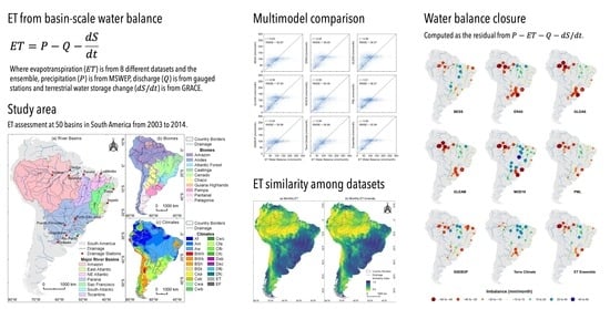
2.1. Study Area

South America is characterized by a wide range of climate regimes and biomes, with three major climate zones (tropical, arid, and temperate climates), from the humid tropics with equatorial climates to temperate and cold arid zones in the southern part of the continent [56], encompassing several major biomes, including the Amazon, Andes, Atlantic Forest, Caatinga, Cerrado, Chaco, Pampa, Pantanal and Patagonia [57,58]. The largest biome in South America is the Amazon, which has undergone in recent years high rates of deforestation and significant changes in surface–atmosphere feedback [59,60,61]. The Amazon biome is characterized by a tropical humid climate and low seasonal temperature variability [62]. The Cerrado biome is characterized by savanna vegetation with a tropical seasonal (wet-to-dry) climate [63]. The Caatinga biome, located in northeast Brazil, is described as a seasonally dry tropical forest with arid and semiarid hot climates [63]. In addition, the Chaco biome, located mostly in Argentina but also in Paraguay and Bolivia, is also described as a dry tropical forest (the largest in South America), with a semiarid climate [64]. While most of this biome is still native vegetation, around 25% of its area has been cleared for agriculture and livestock production [65,66].
Figure 1. (a) River gauges and associated drainage areas (river basins) used in this study to assess water balance and remote-sensing-based evapotranspiration estimates in South America. The red dots represent the gauge stations used to assess water balance (the bigger dots refer to the gauges used to illustrate the water-balance assessment in the following figures). (b) South American biomes from the Terrestrial Ecoregions of the World [58], with modifications based on Turchetto-Zolet et al. [57]. (c) Koppen’s climate zones in South America [56,63], denoted as follows: tropical rainforest (Af), tropical monsoon (Am), tropical wet savannah (Aw), arid hot (BWh), arid cold (BWk), semiarid hot (BSh), semiarid cold (BSk), temperate dry hot summer (Csa), temperate dry and warm summer (Csb), temperate dry and hot summer (Cwa), temperate dry winter and warm summer (Cwb), temperate dry winter and cold summer (Cwc), temperate without dry season and hot summer (Cfa), temperate without dry season and warm summer (Cfb), temperate without dry season and cold summer (Cfc), cold climate with dry and warm summer (Dsb), cold dry summer (Dsc), cold without dry season and warm summer (Dfb), cold without dry season and cold summer (Dfc), polar tundra (ET), and polar frost (EF).
Remotesensing 14 02526 g001
Some of South American biomes, such as the Cerrado, the Pantanal (one of the largest wetland complexes on Earth), and the Atlantic Forest (which has both tropical and subtropical humid climates) are facing environmental and economic threats, including deforestation, fire, cropland expansion, and drought occurrences [67,68,69]. The Pampa biome, located in Southern Brazil, Uruguay, and Argentina, has a seasonal (cold and hot) subtropical climate and temperate grassland vegetation [70], playing an important role in cropland production. Finally, Patagonia reaches the extreme south of South America, and is mainly covered by temperate grassland and steppe vegetation interspersed with shrubs characterized by temperate and arid cold climates [56].

2.2. Global Evapotranspiration Datasets

A total of eight global datasets were used in this study (Table 1), which were divided into two approaches: (i) remote-sensing-based, and (ii) comprehensive-model-based, including land-surface models, biophysical processes, and simplified water-balance approaches. We also computed the ensemble mean ( E T e n s ) as the arithmetic average of all available E T g l datasets. Given data availability, we used the 2003–2014 period to assess E T g l estimates in South America.

2.2.1. Remote-Sensing-Based Datasets

Four E T g l datasets relied primarily on remote sensing, which can be divided into vegetation ( V I )-based and surface temperature ( T s )-based methods. V I -based methods include the Global Land Evaporation Amsterdam Model (GLEAM) [26,71], MOD16 [25,72] and Penman-Monteith-Leuning (PML) [73], while ( T s )-based ones are represented here by the operational Simplified Surface Energy Balance (SSEBOP) algorithm [24,74].
Table 1. Summary of global evapotranspiration datasets assessed in this study.
ModelMethodsSpatial ResolutionTemporal
Resolution
Remote Sensing SourceRemote Sensing DriversMeteorological DriversReferences
BESSBiophysical process-based model5 km8 daysMODISAtmospheric data (aerosol, water vapor, cloud, atmospheric profile)
Surface properties (surface temperature, land cover, leaf area index, albedo)
Global meteorology (MODIS, ERA Interim and NCEP/NCAR)Jiang and Ryu [75];
Ryu et al. [18]
ERA5
(v. Land)
Land-surface model
(CHTESSEL)
0.1 degreeHourlyMODIS, SPOT-VegetationVegetation phenology (leaf area index, vegetation index)
Surface properties (land cover)
Global meteorology (ERA5)Hersbach et al. [35];
Nogueira et al. [76]
GLDAS
(v. 2.1)
Land-surface model
(NOAH)
0.25 degree3-hourlyMODIS
GPCP
Surface properties
Precipitation
Global meteorology (AGRMET) and global data assimilation (GDAS)Rodel et al. [34]
GLEAM
(v. 3.3b)
Remote sensing (Priestley–Taylor equation)0.25 degreeDailyAIRS, CERES, MODIS, ESA-CCI, SMOSAtmospheric data (radiation, precipitation, air temperature, lightning frequency)
Surface properties (snow water equivalent, multisource soil moisture, vegetation cover fraction, vegetation optical depth)
--Martens et al. [71];
Miralles et al. [26]
MOD16
(v. 6)
Remote sensing (Penman–Monteith equation)500 m8 daysMODISVegetation phenology (leaf area index)
Surface properties (land cover, albedo, emissivity)
Global meteorology (MERRA-2)Mu et al. [25,77]
PML
(v. 2)
Remote sensing (Penman–Monteith equation)500 m8 daysMODISVegetation phenology (leaf area index, fraction of photosynthetically active radiation)
Surface properties (land cover, albedo)
Global meteorology (GLDAS)Zhang et al. [73]
SSEBOP
(v. 4)
Remote Sensing (Simplified surface energy balance)1 kmMonthlyMODISThermal data (land surface temperature)
Multispectral data (surface reflectance)
Global meteorology (GLDAS)Senay et al. [24,78]
Terra ClimateOne-dimensional water balance (modified Thornthwaite–Mather equation)2.5 arcminMonthly----Global meteorology (WorldClim and JRA55)Abatzoglou et al. [29]
GLEAM is based on the Priestley–Taylor equation and was developed to estimate surface evaporative fluxes at a spatial resolution of 0.25° and daily temporal resolution [26,71]. GLEAM estimates canopy transpiration, bare-soil evaporation, canopy interception and open-water evaporation, combining multiple sources of data, including snow-water equivalent, soil moisture, and vegetation optical depth and vegetation cover fraction. The algorithm also provides a root-zone soil-moisture profile, infiltration, and evaporative stress conditions, used as constraints on soil evaporation and canopy transpiration. GLEAM version 3.3.b adopted here uses only remote-sensing observations (optical and microwave datasets, and dynamic land-cover classification), including data from CERES (Clouds and Earth’s Radiant Energy System), AIRS (Atmospheric Infra-Red Sounder), SMOS (Soil Moisture and Ocean Salinity) and ESA-CCI (European Space Agency—Climate Change Initiative) [26,71].
MOD16 [25,72] is based on the Penman–Monteith equation and uses vegetation indices to estimate canopy conductance. The total E T includes soil and canopy evaporation, and canopy transpiration at a spatial resolution of 500 m and temporal resolution of 8 days. To estimate E T , the algorithm includes remote-sensing and global meteorological reanalysis data. Remote-sensing inputs that represent land-surface processes are derived from the Moderate Resolution Imaging Spectroradiometer (MODIS) datasets, including land-cover classification, leaf area index ( L A I ), fraction of photosynthetically active radiation ( f P A R ), and albedo. As meteorological inputs, the algorithm uses reanalysis from MERRA-2 (Modern-Era Retrospective analysis for Research and Applications), with spatial resolution of 0.5° × 0.65°. To combine meteorological and remote-sensing inputs, meteorological data are interpolated from coarse spatial resolution to match THE MODIS spatial resolution and to remove abrupt changes from the meteorological reanalysis data [79].
PML [73] is a physically based model that estimates E T using the Penman–Monteith equation. Input data are from MODIS, including L A I , albedo, and emissivity, while meteorological inputs are from the Global Land Data Assimilation System (GLDAS) rescaled to 500 m using a bilinear interpolation. PML computes total E T by accounting for the evaporation from soil and canopy interception and vegetation transpiration. Spatial and temporal resolution are 500 m and 8 days, respectively.
SSEBOP [24,78] is based on a simplified SEB approach with a simple parameterization for operational applications. The algorithm combines E T fractions derived from T s and surface reflectance from MODIS and meteorological reanalysis from GLDAS. The one-source algorithm estimates total E T at a spatial resolution of 1 km and monthly temporal resolution.

2.2.2. Comprehensive-Model-Based Approaches

Four E T g l datasets were based on land-surface models, including ERA5 [35,80] and GLDAS [34]; biophysical-process-based models, including the Breathing Earth System Simulator (BESS) [18,75]; and simplified water-balance approaches from Terra Climate [29]. ERA5 is a global atmospheric-reanalysis dataset [35,80] generated by the European Centre for Medium-Range Weather Forecasts (ECMWF). ERA5 combines observed and simulated data to estimate meteorological parameters. ERA5-Land uses the ECMWF land-surface model Carbon Hydrology-Tiled Scheme for Surface Exchanges over Land (CHTESSEL) to compute hydrological fluxes [76]. Vegetation characteristics are derived from global land-cover datasets, while vegetation density and phenology are obtained from lookup tables as a function of the respective dominant type of vegetation [76]. The dataset is available at hourly, daily, and monthly temporal resolutions, with a spatial resolution of 0.1°.
GLDAS reanalysis dataset [34] is based on in situ and remote-sensing datasets, including MODIS and Global Precipitation Climatology Project (GPCP), forced with the Global Data Assimilation System (GDAS) and Agricultural Meteorological Modeling System (AGRMET). GLDAS includes four different land-surface models, and in this study we used NOAH, which uses a Penman–Monteith approach to compute potential E T ( P E T ) with a parameterization based on surface–atmosphere interactions, vegetation conditions, and water availability to estimate actual E T . GLDAS is available at 3-hourly, daily, and monthly temporal resolutions, with a spatial resolution of 0.25°.
The Breathing Earth System Simulator (BESS) is a process-based model designed to estimate E T and gross primary productivity at global scale with fine spatial resolution [18,75]. It couples a one-dimensional atmospheric radiative transfer module, a two-leaf canopy radiative transfer module, and an integrated carbon assimilation and energy balance module, fully based on MODIS land-surface ( T s , land cover, LAI, albedo) and atmospheric (aerosol, water vapor, cloud, atmospheric profile) datasets. It uses global meteorology from ERA-Interim to gap-fill missing atmospheric data, and global reanalysis from the National Center for Environmental Prediction–National Center for Atmospheric Research (NCEP-NCAR) to compute aerodynamic resistances. The spatial and temporal resolution of the adopted BESS dataset is 5 km and 8 days, respectively.
Terra Climate [29] is a monthly climate dataset that spans from 1958 to present, based on the high-spatial-resolution WorldClim climate data, in addition to Climate Research Unit (CRU) and Japanese 55-year Reanalysis (JRA55) datasets. E T is computed from a one-dimensional simplified water balance based on a modified Thornthwaite–Mather approach, that uses P , P E T (calculated using Penman–Monteith equation), soil moisture, and snowpack water storage. The model data are available at a monthly temporal resolution and 2.5 arcminutes spatial resolution.

2.3. Water-Balance Estimation of Evapotranspiration

We computed E T w b , from 2003 to 2014, as the residual of the water-balance equation (Equation (1)).
E T w b = P Q d S d t
where P was taken from Multi-Source Weighted-Ensemble Precipitation (MSWEP) version 2.2 [81,82], d S / d t from Gravity Recovery and Climate Experiment (GRACE) [83,84,85] and Q measurements from the Brazilian Water and Sanitation Agency (ANA) and the Argentinian Hydrological Database System (SNIH).
MSWEP dataset was designed specifically for hydrological modeling and assessment, with a spatial resolution of 0.1° and temporal resolution from 3 h to 30 days. MSWEP merges multiple high-quality P datasets, including measurements, satellite observations, and reanalysis data [81,82].
Monthly Q was integrated from daily streamflow measurements from ANA (available at https://www.snirh.gov.br, last accessed on 18 August 2021) and SNIH (available at https://snih.hidricosargentina.gob.ar/, last accessed on 18 August 2021). We did not gap-fill the data, so we selected basins with complete data, and months with missing data were excluded from analysis. All stations used to compute the water balance are presented in Supplementary Information Table S1.
Changes in storage ( d S / d t ) were computed using changes in terrestrial water storage ( T W S ) from GRACE, which detects changes in the Earth’s gravitational field by measuring the distance between two orbiting satellites [83,84,85] (Equation (2)). The available GRACE T W S data are anomalies relative to the 2004–2009 time-mean baseline, with a spatial resolution of 1° in both latitude and longitude, and monthly temporal resolution (approximately). Considering the irregular time intervals, we computed these changes as the difference between two GRACE observations (t + 1 and t), representing the average change in T W S [86].
d S d t Δ T W S Δ t T W S t + 1 T W S t Δ t
We used a simple average of the three different GRACE spherical harmonic solutions (from GFZ (GeoForschungsZentrum), CSR (Center of Space Research from the University of Texas), and NASA JPL (Jet Propulsion Laboratory)) to reduce the noise in the gravity fields [87].

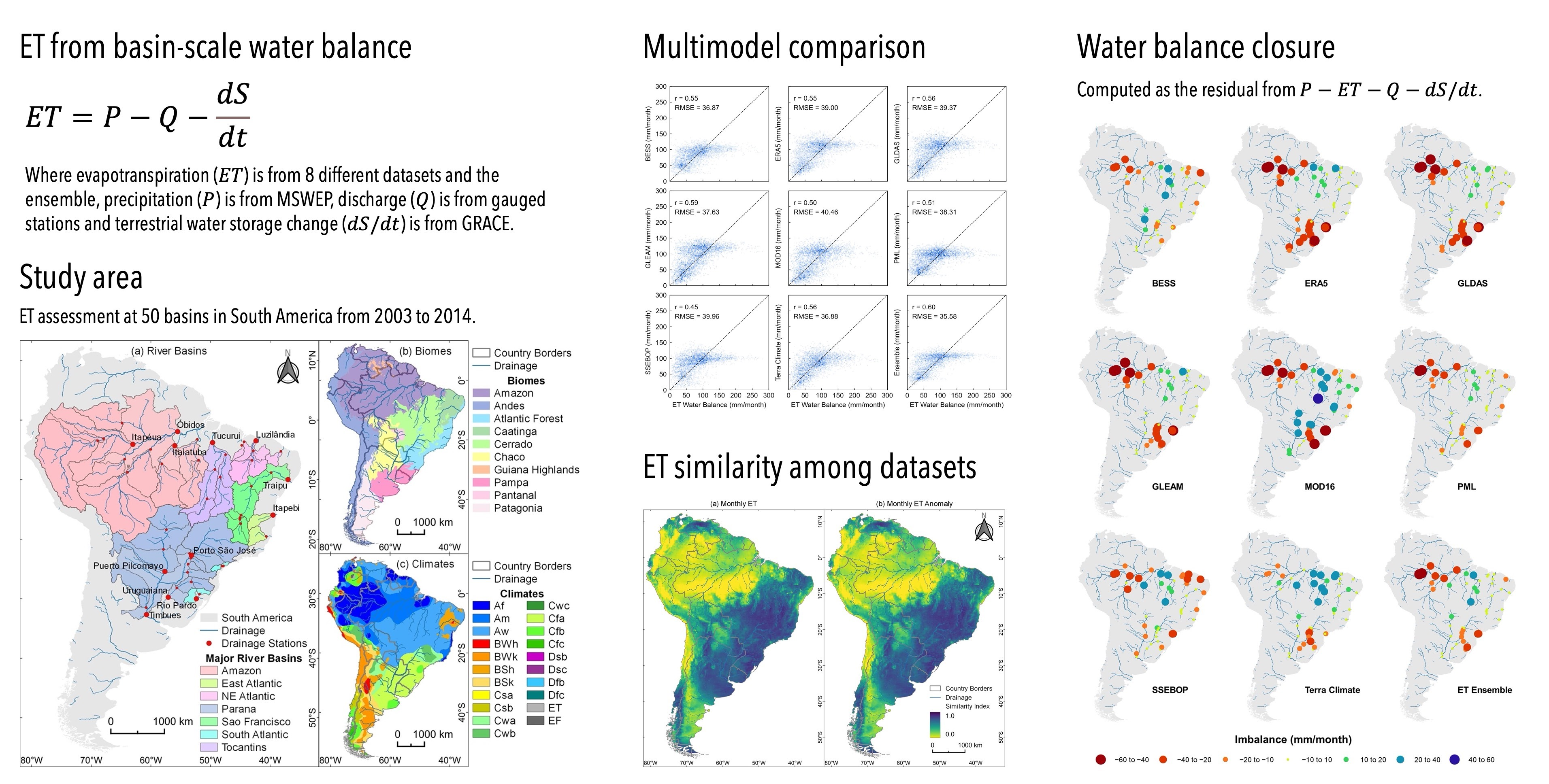
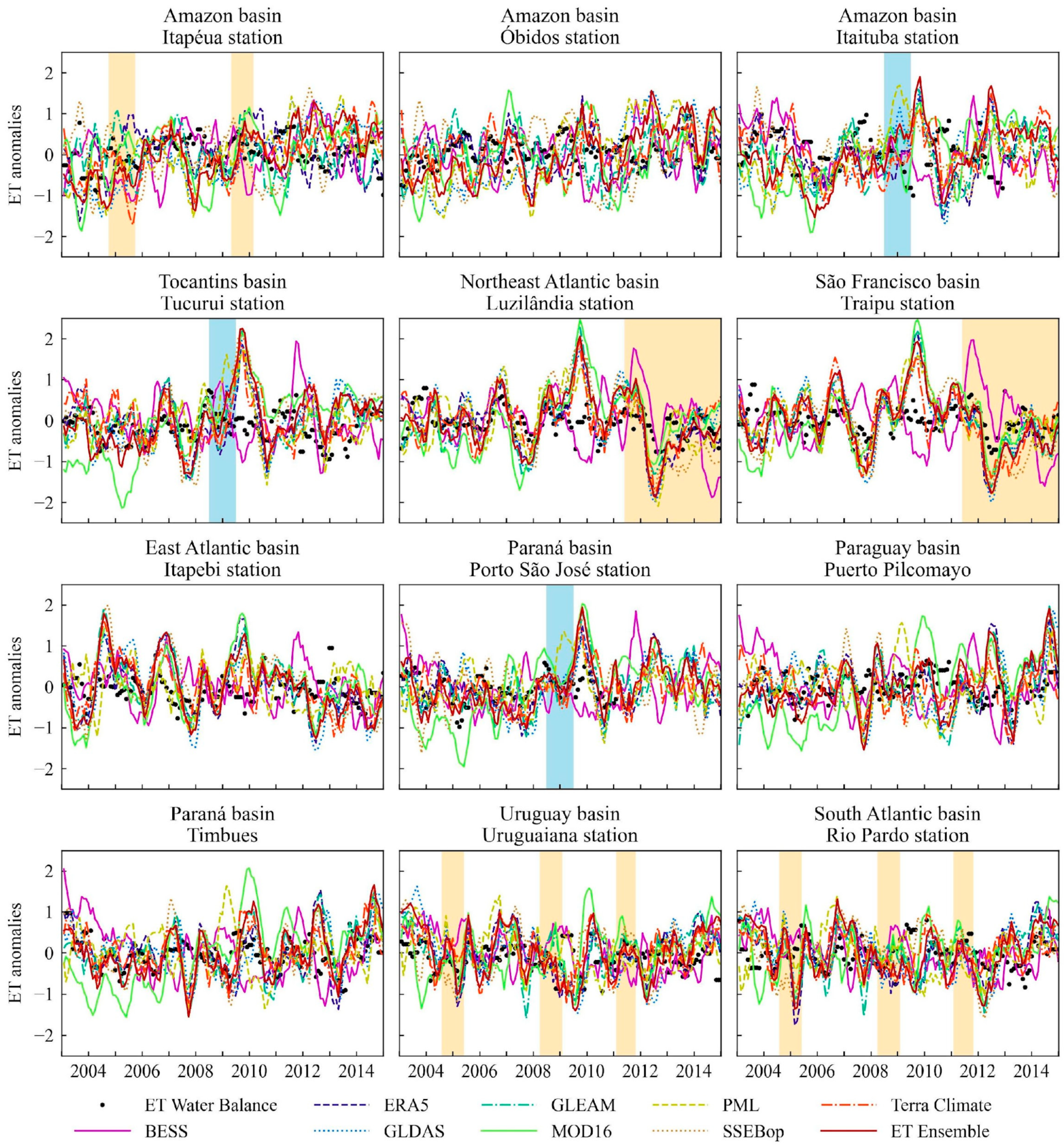
2.4. Seasonal and Interannual Assessments of Evapotranspiration

To remove the seasonal cycle of the E T estimations and compute ET anomalies, we standardized the time series by subtracting the monthly long-term average from each monthly E T estimate, dividing by the standard deviation [88]. To assess the agreement in terms of average, phase, and amplitude between the E T time series derived from multiple global datasets, we computed the similarity index ( Ω ) [46,89] for monthly E T and monthly E T anomaly (Equation (3)).
Ω = m σ b 2 σ 2 ( m 1 ) σ 2
where m is the number of ensemble members ( m = 8 ), σ b 2 is the ensemble variance of the time series, and σ 2 is the total variance of all ensemble members concatenated. A value of Ω equal to 1 indicates identical series, whereas values around 0 indicate poor-to-no agreement. Although values below zero are mathematically possible, they are very unlikely to happen, especially with an increasing number of members (m) [89].

2.5. Assessment of the Accuracy of Global Evapotranspiration

To compare E T g l and E T w b , we resampled all global ET datasets to monthly time scales and then we aggregated the basin-wide E T using a simple average, since this scheme has the best performance in preserving the mass balance [90]. To assess the accuracy of the E T g l estimates, we used nonprobabilistic metrics [88] of Pearson’s coefficient of correlation (r), bias, and root-mean-squared error (RMSE) between E T w b and E T g l .

3. Results and Discussion

3.1. Evapotranspiration Comparison between Water Balance and Global Datasets

To assess how consistent E T g l estimates are on a monthly time scale, a comparison between the water-balance approach and global datasets is presented in Figure 2. Results showed moderate correlation coefficients, with values ranging from 0.45 (SSEBOP) to 0.60 ( E T e n s ), while RMSE ranged between 35.6 ( E T e n s ) and 40.5 (MOD16) mm·month−1. E T g l rates ranged between 0 and 150 mm·month−1 in most basins, while E T w b estimates presented maximum rates up to 250 mm·month−1. Overall, E T e n s performed slightly better than the other global datasets, yielding correlations around 0.60 and RMSE of 35.6 mm·month−1. From an assessment based on major basins (Supplementary Information Table S2), two main results can be highlighted: (i) basins located in humid climates (including the Amazon, Uruguay, and South Atlantic basins) exhibited weaker correlation, with average values ranging between 0.37 and 0.48 (between 0.17 and 0.56 in the Amazon, and between 0.37 and 0.51 in the Uruguay and South Atlantic basins), with average RMSE around 39.6 mm·month−1 and bias between 11.6 and 23.4 mm·month−1; and (ii) tropical and semiarid basins located in areas where P has a strong seasonality (including the São Francisco, Northeast Atlantic, Paraná/Paraguay, and Tocantins basins), exhibited stronger correlation, with average values ranging between 0.59 and 0.81, average RMSE between 32.5 and 43.1 mm·month−1, and smaller negative bias ranging between 1 and −14 mm·month−1. These differences may be related to different E T driving factors. While in the Amazon and other basins located in Southern Brazil, E T is mainly driven by available energy (with global radiation showing a strong seasonality in the Uruguay and South Atlantic basins) [91,92,93], in the northeast and central areas of Brazil, water availability is the main driver [91,94,95]. Therefore, our results suggest that global E T datasets have closer agreement with E T w b in basins with stronger P seasonality, where E T is mainly driven by water availability, while in basins with humid climate, global ET products yield a low range of seasonal variation due to abundant water availability.
A statistical assessment based on all 50 basins is summarized in Figure 3. Overall, our results indicate a slight overestimation by most E T g l models compared to E T w b , with median bias ranging between −2.4 and 11.2 mm·month−1 and an interquartile range between −20 (for MOD16) and 30 (for ERA5) mm·month−1. In addition, median RMSE smoothly ranged between 34.8 and 39.7 mm·month−1, with some models showing a higher interquartile range (e.g., ERA5, GLDAS, GLEAM), with errors up to 60 mm·month−1. However, higher correlation values were found for ERA5, GLEAM, MOD16, and E T e n s (median higher than 0.7), while the other E T g l models showed median correlations between 0.51 and 0.65). Overall, our results suggest small discrepancies between global datasets, although some models performed slightly better than others, similarly to other reported results [41]. In the long term, all E T datasets presented moderate-to-low bias, with higher bias in humid climates, despite some of the datasets having high monthly errors, similarly to results found in other studies [41,51].

3.2. Seasonal and Interannual Assessment of Evapotranspiration

The long-term E T seasonal average for the 2003–2014 period is presented in Figure 4 for major South American basins, where E T w b standard deviations are highlighted as shaded areas. Most E T g l presented a similar seasonal pattern in the assessed basins, with E T estimates generally falling within the E T w b deviation range. In basins where P presents a stronger seasonality (i.e., Tocantins, Northeast Atlantic, São Francisco, and Paraná), our results indicate a closer agreement between E T w b and E T g l , yielding a similar seasonal pattern with smaller E T values during the dry season and its smaller deviation. In these basins we found a predominant underestimation (during the wet season and wet-to-dry seasons transition), with average bias between −30 (at Tocantins, for MOD16) and 19 mm·month−1 (at Northeast Atlantic, for SSEBOP). In addition, SSEBOP estimated higher E T rates during the dry season in semiarid climates, especially in the São Francisco and Northeast Atlantic basins, while all other models agreed and yielded lower rates during the dry season. Some overestimation was also found in subtropical humid basins such as the Uruguay and South Atlantic basins, mostly during summer months, with average bias between 7 and 36 mm·month−1 and up 29 mm·month−1, respectively.
In the humid equatorial climate zone, especially in the Amazon Basin, where water availability is not a limiting factor, since P is relatively well-distributed throughout the year, and available energy is the main driver for E T [92], the seasonal pattern shown by the E T w b was not followed by most of the E T g l , with models showing different timing and magnitude when compared to E T w b , as previously discussed [92]. Overall, our results show that E T g l is overestimated in the humid tropics (mainly in central-west Amazon, such as Itapeua and Obidos, with bias between 2.5 and 51.8 mm·month−1) when compared to E T w b , even though an underestimation is seen in eastern parts of the basin (at Itaituba) mostly during the wet season (average bias between −8 and 46 mm·month−1). This could be due to the largest P contribution on the terrestrial water balance; consequently, P variations will strongly affect the E T w b patterns [47]. As in the mainly humid Amazon region, ET is not only controlled by P and water availability, but also by radiation and vegetation phenology [92]; consequently, the water-balance approach will be less accurate in humid tropics [51].
Based on an assessment of the seasonal and interannual variability (Figure 5), a strong disagreement between E T w b and E T g l estimates was found in the Amazon Basin, leading to a wide range of variability. On the other hand, in tropical, subtropical, and semiarid basins (including the Tocantins, São Francisco, Paraná, Paraguay, Uruguay and Atlantic basins), a stronger agreement was found. Despite the wide range of variability, most models agreed in positive anomalies during the drought of 2010 (Amazon at Itapeua) [96,97] and during the anomalously wet year of 2009 (at Itaituba) [98,99,100], while E T w b showed negative anomalies in the same period.
In tropical and semiarid climates (Tocantins, São Francisco, Northeast Atlantic, Paraná and Paraguay basins), we found moderate-to-strong agreements between global E T g l and E T w b estimates for most of the E T models and the ensemble mean. Most of the E T g l datasets accurately represented wet and dry anomalous events in these climates. For the long-lasting floods of 2009–2010 that affected the Amazon region, including the Tocantins (at Tucuruí) [98] and the Paraná (at Porto São José) [101] basins, all models consistently estimated a positive E T anomaly over the flooding period, in agreement with water-balance estimates. Another hydrological extreme event well-captured by global models was the long drought that affected the Northeast region in Brazil over the 2012–2016 period [100], in the Northeast Atlantic and São Francisco basins (at Luzilândia and Traipu), with negative strong anomalies being observed since 2012. Furthermore, in subtropical humid climates, drought events that occurred in Southern Brazil (Uruguay and South Atlantic basins) over 2005, 2009, and 2012 [96], were only partially represented by E T g l datasets. Overall, most of the global E T datasets yielded a moderate agreement with E T w b ; however, in some situations, MOD16, GLDAS, and SSEBOP showed a higher amplitude of anomalies than other models in most of the basins. SSEBOP showed higher variations than other models in the Northeast Atlantic basin (at Luzilandia) for both positive and negative anomalies. MOD16 showed negative anomalies before 2007/2008 and positive anomalies for 2009–2012 in Paraguay (at Puerto Pilcomayo), and Paraná (at Timbues) basins, in contrast to other global models. This MOD16 behavior resulted in a positive E T trend. Similar results were previously reported in the Pantanal biome, with changes in the interannual variability from 2001–2006 to 2007–2012 [102]. MOD16 errors may arise from the algorithm structure [103], meteorological forcing data and possible biases [25,104], and land-cover parameterization [105], and further research is needed to identify this source of uncertainties.
From a climatic viewpoint of water-limited versus energy-limited E T estimates in South America, an assessment based on the agreement among the global datasets, represented by the similarity index Ω (Figure 6a), indicates (i) higher similarity ( Ω higher than 0.7) from the northeast to the southeast parts of the continent, including the Cerrado, Caatinga, Pantanal, Atlantic Forest, and Pampa biomes, where E T is driven by water and radiation combined [46]; (ii) lower similarity ( Ω between 0.2 and 0.4) in the extreme south of the continent, in the Patagonia biome, where E T is mainly driven by water availability [46]; and (iii) very low similarity ( Ω lower than 0.2) in the Amazon biome and Andes regions, where E T is mainly driven by radiation [46], but also by a combination with radiation and vegetation phenology [92]. The similarity of seasonal variability ( E T monthly anomalies, Figure 6b) is relatively higher in northeast Brazil (Caatinga biome) and in central parts of Brazil (Cerrado biome), while moderate similarity was found in southern Brazil (Pampa biome, including areas in Central Argentina, and Uruguay), and lower similarity was found in the Amazon.
In some regions, as in southeastern, central, and northeastern Brazil, the global E T datasets consistently agree on monthly E T , but to a lower degree on E T anomalies. Some opposite behavior was found for the Amazon and Patagonia, with higher agreement on monthly anomalies. Considering different dataset sources (remote-sensing-driven models, including GLEAM, MOD16, PML, and SSEBOP; and reanalysis, land-surface, and process-based models, including BESS, ERA5, GLDAS, and Terra Climate), a slightly higher similarity was found for the second group of assessed models for both monthly E T and E T anomalies in the Amazon (Supplementary Information Figure S1). Our findings are similar with another study [46], even though different E T datasets were used. As they indicate, when the similarity is higher, less uncertainty is found, and thus the selection of a particular dataset is less important, while when the similarity of E T anomalies is higher, seasonal variability is better represented by the models, which can be important for studies where this is of particular interest.

3.3. Water-Balance Closure

We assessed the water-balance closure (imbalance) using monthly averages from 2003 to 2014 as P E T Q d S / d t , considering E T estimates from the global datasets. Figure 7 summarizes the spatial variability of the long-term average (2003–2014) imbalance for major South American hydrological regions. There is a larger imbalance in the Amazon basin, and most global models showed a negative imbalance in the western Amazon (Itapeua and Obidos) and a positive imbalance in the eastern Amazon (Itaituba). The water balance using BESS, PML, SSEBOP, and Terra Climate models led to the lowest imbalance range in the Amazon. The other tropical basins exhibited a smaller positive imbalance. For the Tocantins basin, most global models showed an imbalance average of around 13 mm·month−1, ranging between 6 and 17.8 mm·month−1, except MOD16, whose median value was 30.2 mm·month−1. In the Paraná Basin, the median imbalance ranged between −18 mm·month−1 and 11.5 mm·month−1, with BESS, E T e n s , PML, SSEBOP, and Terra Climate yielding imbalances lower than 5 mm·month−1. In the São Francisco basin, E T g l showed an average imbalance from 3 to 11 mm·month−1, except MOD16, which showed a larger imbalance (median of 21 mm·month−1). In the Northeast Atlantic basin, SSEBOP showed an average imbalance around −19 mm·month−1, while for the other models the average imbalance ranged from −8 to 9 mm·month−1. Basins located in Southern Brazil (South Atlantic and Uruguay) showed lower imbalance values for BESS, PML, and SSEBOP models (average imbalance from −7 to −17 mm·month−1), while with the other models a higher imbalance was verified (higher than −20 mm·month−1).
From the spatial assessment of the long-term water-balance closure (Figure 7, three main results can be highlighted: (i) in the Amazon basin, our results showed higher negative imbalances, ranging from −60 up to 20 mm·month−1 using most of the E T g l datasets; (ii) in the southern basins (Uruguay and South Atlantic), higher negative imbalances were also found, mainly for ERA5, GLDAS, GLEAM, and MOD16; and (iii) most of the E T g l datasets yielded lower imbalance, ranging between −10 to 20 mm·month−1 in basins located in tropical and semiarid climates (Northeast Atlantic and São Francisco basins), with MOD16 showing higher positive imbalances. Overall, despite some differences among all global models, the long-term water-balance closure demonstrated similar patterns over South American basins, with higher imbalance in the humid tropics and lower imbalance in tropical and semiarid climates. Overall, our results agree with other research findings, indicating that E T datasets demonstrate hydrological consistency, especially in water-limited conditions, while in humid climates, biases are relatively higher [51]. Furthermore, our results also indicate similarities between different approaches to estimate E T , with no obvious divergences, since most of the models yielded similar statistics. Some models performed relatively better than others, which was concluded in previous studies [41].

4. Conclusions

The main goal of this research paper was to assess publicly available and easily accessible global E T datasets across multiple climate conditions in South America. We evaluated eight global E T datasets based on remote-sensing, reanalysis, land-surface, and biophysical-process-based modeling, as well as the ensemble mean, and compared them with ET estimated from water balance in 50 medium-to-large basins to answer the following questions:
i. 
How consistent are  E T  estimates from global datasets based on remote-sensing, reanalysis, land-surface, and biophysical models when compared to  E T w b ?
Our results indicate similar errors when E T g l are compared with the water-balance approach ( E T w b ), with moderate correlations and a slight tendency of overestimation in most of South American climates. However, basins located in tropical (and subtropical) humid climates presented lower accuracy and weaker correlations when compared to basins located in tropical seasonal (wet-to-dry) and semiarid climates, suggesting that global E T datasets have closer agreement with E T w b in basins with stronger P seasonality, when E T is mainly driven by water availability.
ii. 
Do they coherently represent its magnitude and seasonality?
Most E T g l presented a similar seasonal pattern in the assessed basins, with E T estimates generally falling within the E T w b deviation range, with basins located in tropical seasonal (wet-to-dry) climates achieving a closer agreement. Nevertheless, in humid climates (especially in the tropics) we found higher differences, with E T g l yielding different timing and magnitude when compared to E T w b , with an overall tendency of overestimation.
iii. 
How do they agree in terms of seasonal and interannual variability?
Our results indicate a strong disagreement in the seasonal and interannual variability between E T w b and E T g l in the humid tropics. However, in tropical seasonal (wet-to-dry) and subtropical climates, we found higher agreement between E T g l for detection of wet and dry anomalous events. These findings also agree with the similarity assessment, with lower similarity in the humid tropics (Amazon biome) and higher similarity in the Cerrado, Caatinga, Pantanal, Atlantic Forest and Pampa biomes. Overall, similarities were higher for monthly E T than monthly anomalies in these biomes.
The spatial and temporal assessment of the water-balance closure indicated a moderate hydrological consistency in the long-term annual average for most of the E T g l , including E T e n s ; however, higher imbalances were found in the humid tropics and subtropics. Improvements are needed to achieve lower uncertainties and higher accuracy of ET estimates mostly in the humid tropics, especially for seasonal and interannual variability. The use of E T e n s can reduce uncertainties related to single models and their forcing data [41], improving the quality of E T estimates at regional and continental scales for water management purposes [1]. E T estimates based on multiple models can also be enhanced based on spatial refinements of the water-balance approach and the use of eddy covariance networks to better understand E T drivers and thus improve models’ calibration and validation [55].
Achieving a consistent large-scale water-balance closure still remains a challenge in the humid tropics, and optimization strategies could be used to improve E T estimates [106], and its seasonal and interannual variability [107]. Assessing the sources of uncertainties in the water-balance approach from all hydrological variables is a critical issue that deserves further investigation, especially to achieve a higher accuracy on each water cycle component and to consistently close the water balance [55]. However, results from this study provided important information about the E T dynamics at basin scale and a basis for the future development of optimized E T based on the combination of multiple datasets at continental scale in South America. Therefore, future research is needed to improve E T estimates for water resources management and hydrological applications.

Supplementary Materials

The following are available online at https://www.mdpi.com/article/10.3390/rs14112526/s1: Figure S1: Similarity index for all global evapotranspiration datasets, remote-sensing-based models, including GLEAM, MOD16, PML, and SSEBOP, and land-surface, process-based models, and simplified water balance, including BESS, ERA5, GLDAS, and Terra Climate. Maps are provided for monthly absolute and monthly anomaly evapotranspiration estimates. Table S1: Summary of the discharge stations used to assess the water-balance evapotranspiration in major South American river basins. Table S2: Summary of the statistical assessment by evapotranspiration model and by major basins in South America.

Author Contributions

Conceptualization, A.A.M., A.R. and A.S.F.; methodology, A.A.M., A.R. and R.B.; programming, A.A.M., L.L. and R.B.; data curation and formal analysis, A.A.M., A.R., B.C.d.A., L.L. and R.B.; validation, A.A.M., A.R., A.S.F., B.C.d.A., L.L. and R.B.; discussions, A.A.M., A.R., L.L., B.C.d.A., R.B., G.L.C., G.M.R.F., V.A.S., J.P.L.F.B., R.C.D.d.P., A.M., A.d.A.T., A.A.A., M.A.F. and T.B.; writing—A.A.M., A.R., A.S.F., B.C.d.A., G.L.C., L.L., R.B. and V.A.S.; writing—review and editing, A.A.M., A.R., B.C.d.A., L.L., R.B., G.L.C., G.M.R.F., V.A.S., J.P.L.F.B., R.C.D.d.P., A.M., A.d.A.T., A.A.A., M.A.F. and T.B.; visualization, A.A.M., A.R., G.L.C., L.L., B.C.d.A. and R.B.; supervision, A.R. and R.C.D.d.P.; project administration, A.R. and R.C.D.d.P.; funding acquisition, A.R. and R.C.D.d.P. All authors have read and agreed to the published version of the manuscript.

Funding

The authors would like to gratefully acknowledge the financial support provided by the Brazilian Agency for the Improvement of Higher Education (CAPES) and the Brazilian National Water and Sanitation Agency (ANA) in the context of the projects “Estimating land surface evapotranspiration using remote sensing models for water management in Brazil”, and “Technological Cooperation for Hydrological Assessments in Brazil—Environmental and Economical Water Accounting”, numbers 88881.178687/2018-01 and TED-05/2019-ANA, respectively. A.A.M., A.S.F. and V.A.S were supported by National Council for Scientific and Technological Development (CNPq). L.L and J.P.L.F.B were supported by Higher Education Improvement Coordination (CAPES). T.B. was funded in part by National Science Foundation award number BCS-1825046.

Data Availability Statement

The data that support the findings of this study, including discharge stations, river basins and measured discharge, are freely available at https://metadados.snirh.gov.br/ or upon request to the corresponding author.

Acknowledgments

The authors would like to thank the Federal University of Rio Grande do Sul (UFRGS) and the Brazilian Water and Sanitation Agency (ANA) for institutional support.

Conflicts of Interest

The authors declare no conflict of interest.

References

  1. Elnashar, A.; Wang, L.; Wu, B.; Zhu, W.; Zeng, H. Synthesis of global actual evapotranspiration from 1982 to 2019. Earth Syst. Sci. Data 2021, 13, 447–480. [Google Scholar] [CrossRef]
  2. Wright, J.S.; Fu, R.; Worden, J.R.; Chakraborty, S.; Clinton, N.E.; Risi, C.; Sun, Y.; Yin, L. Rainforest-initiated wet season onset over the southern Amazon. Proc. Natl. Acad. Sci. USA 2017, 114, 8481–8486. [Google Scholar] [CrossRef] [PubMed] [Green Version]
  3. Fisher, J.B.; Malhi, Y.; Bonal, D.; Da Rocha, H.R.; De Araújo, A.C.; Gamo, M.; Goulden, M.L.; Rano, T.H.; Huete, A.R.; Kondo, H.; et al. The land-atmosphere water flux in the tropics. Glob. Chang. Biol. 2009, 15, 2694–2714. [Google Scholar] [CrossRef]
  4. Zemp, D.C.; Schleussner, C.-F.; Barbosa, H.M.J.; van der Ent, R.J.; Donges, J.F.; Heinke, J.; Sampaio, G.; Rammig, A. On the importance of cascading moisture recycling in South America. Atmos. Chem. Phys. 2014, 14, 13337–13359. [Google Scholar] [CrossRef] [Green Version]
  5. Martinelli, L.A.; Naylor, R.; Vitousek, P.M.; Moutinho, P. Agriculture in Brazil: Impacts, costs, and opportunities for a sustainable future. Curr. Opin. Environ. Sustain. 2010, 2, 431–438. [Google Scholar] [CrossRef]
  6. Spera, S.A.; Galford, G.L.; Coe, M.T.; Macedo, M.N.; Mustard, J.F. Land-use change affects water recycling in Brazil’s last agricultural frontier. Glob. Chang. Biol. 2016, 22, 3405–3413. [Google Scholar] [CrossRef]
  7. Bojinski, S.; Verstraete, M.; Peterson, T.C.; Richter, C.; Simmons, A.; Zemp, M. The Concept of Essential Climate Variables in Support of Climate Research, Applications, and Policy. Bull. Am. Meteorol. Soc. 2014, 95, 1431–1443. [Google Scholar] [CrossRef]
  8. Hollmann, R.; Merchant, C.J.; Saunders, R.; Downy, C.; Buchwitz, M.; Cazenave, A.; Chuvieco, E.; Defourny, P.; de Leeuw, G.; Forsberg, R.; et al. The ESA Climate Change Initiative: Satellite Data Records for Essential Climate Variables. Bull. Am. Meteorol. Soc. 2013, 94, 1541–1552. [Google Scholar] [CrossRef] [Green Version]
  9. Sachs, J.D. From millennium development goals to sustainable development goals. Lancet 2012, 379, 2206–2211. [Google Scholar] [CrossRef]
  10. Karimi, P.; Bastiaanssen, W.G.M.; Molden, D.; Cheema, M.J.M. Basin-wide water accounting based on remote sensing data: An application for the Indus Basin. Hydrol. Earth Syst. Sci. 2013, 17, 2473–2486. [Google Scholar] [CrossRef] [Green Version]
  11. Hamilton, K. Measuring Sustainability in the UN System of Environmental-Economic Accounting. Environ. Resour. Econ. 2016, 64, 25–36. [Google Scholar] [CrossRef]
  12. Cuxart, J.; Boone, A.A. Evapotranspiration over Land from a Boundary-Layer Meteorology Perspective. Bound.-Layer Meteorol. 2020, 177, 427–459. [Google Scholar] [CrossRef]
  13. Shrestha, P.; Simmer, C. Modeled Land Atmosphere Coupling Response to Soil Moisture Changes with Different Generations of Land Surface Models. Water 2020, 12, 46. [Google Scholar] [CrossRef] [Green Version]
  14. Pielke, R.A.; Avissar, R.; Raupach, M.; Dolman, A.J.; Zeng, X.B.; Denning, A.S. Interactions between the atmosphere and terrestrial ecosystems: Influence on weather and climate. Glob. Chang. Biol. 1998, 4, 461–475. [Google Scholar] [CrossRef]
  15. Rajib, A.; Evenson, G.R.; Golden, H.E.; Lane, C.R. Hydrologic model predictability improves with spatially explicit calibration using remotely sensed evapotranspiration and biophysical parameters. J. Hydrol. 2018, 567, 668–683. [Google Scholar] [CrossRef] [PubMed]
  16. Nijzink, R.C.; Almeida, S.; Pechlivanidis, I.G.; Capell, R.; Gustafssons, D.; Arheimer, B.; Parajka, J.; Freer, J.; Han, D.; Wagener, T.; et al. Constraining Conceptual Hydrological Models With Multiple Information Sources. Water Resour. Res. 2018, 54, 8332–8362. [Google Scholar] [CrossRef] [Green Version]
  17. Allen, R.G.; Pereira, L.S.; Howell, T.A.; Jensen, M.E. Evapotranspiration information reporting: I. Factors governing measurement accuracy. Agric. Water Manag. 2011, 98, 899–920. [Google Scholar] [CrossRef] [Green Version]
  18. Ryu, Y.; Baldocchi, D.D.; Kobayashi, H.; van Ingen, C.; Li, J.; Black, T.A.; Beringer, J.; van Gorsel, E.; Knohl, A.; Law, B.E.; et al. Integration of MODIS land and atmosphere products with a coupled-process model to estimate gross primary productivity and evapotranspiration from 1 km to global scales. Glob. Biogeochem. Cycles 2011, 25, GB4017. [Google Scholar] [CrossRef] [Green Version]
  19. Pastorello, G.; Trotta, C.; Canfora, E.; Chu, H.; Christianson, D.; Cheah, Y.-W.; Poindexter, C.; Chen, J.; Elbashandy, A.; Humphrey, M.; et al. The FLUXNET2015 dataset and the ONEFlux processing pipeline for eddy covariance data. Sci. Data 2020, 7, 225. [Google Scholar] [CrossRef]
  20. Lettenmaier, D.P.; Alsdorf, D.; Dozier, J.; Huffman, G.J.; Pan, M.; Wood, E.F. Inroads of remote sensing into hydrologic science during the WRR era. Water Resour. Res. 2015, 51, 7309–7342. [Google Scholar] [CrossRef]
  21. Liou, Y.-A.; Kar, S.K. Evapotranspiration Estimation with Remote Sensing and Various Surface Energy Balance Algorithms—A Review. Energies 2014, 7, 2821–2849. [Google Scholar] [CrossRef] [Green Version]
  22. Bastiaanssen, W.G.M.; Menenti, M.; Feddes, R.A.; Holtslag, A.A.M. A remote sensing surface energy balance algorithm for land (SEBAL): 1. Formulation. J. Hydrol. 1998, 212–213, 198–212. [Google Scholar] [CrossRef]
  23. Allen, R.G.; Tasumi, M.; Trezza, R. Satellite-Based Energy Balance for Mapping Evapotranspiration with Internalized Calibration (METRIC)—Model. J. Irrig. Drain. Eng. 2007, 133, 380–394. [Google Scholar] [CrossRef]
  24. Senay, G.B.; Bohms, S.; Singh, R.K.; Gowda, P.H.; Velpuri, N.M.; Alemu, H.; Verdin, J.P. Operational Evapotranspiration Mapping Using Remote Sensing and Weather Datasets: A New Parameterization for the SSEB Approach. JAWRA J. Am. Water Resour. Assoc. 2013, 49, 577–591. [Google Scholar] [CrossRef] [Green Version]
  25. Mu, Q.; Zhao, M.; Running, S.W. Improvements to a MODIS global terrestrial evapotranspiration algorithm. Remote Sens. Environ. 2011, 115, 1781–1800. [Google Scholar] [CrossRef]
  26. Miralles, D.G.; Holmes, T.R.H.; De Jeu, R.A.M.; Gash, J.H.; Meesters, A.G.C.A.; Dolman, A.J. Global land-surface evaporation estimated from satellite-based observations. Hydrol. Earth Syst. Sci. 2011, 15, 453–469. [Google Scholar] [CrossRef] [Green Version]
  27. Jung, M.; Reichstein, M.; Bondeau, A. Towards global empirical upscaling of FLUXNET eddy covariance observations: Validation of a model tree ensemble approach using a biosphere model. Biogeosciences 2009, 6, 2001–2013. [Google Scholar] [CrossRef] [Green Version]
  28. Jung, M.; Reichstein, M.; Margolis, H.A.; Cescatti, A.; Richardson, A.D.; Arain, M.A.; Arneth, A.; Bernhofer, C.; Bonal, D.; Chen, J.; et al. Global patterns of land-atmosphere fluxes of carbon dioxide, latent heat, and sensible heat derived from eddy covariance, satellite, and meteorological observations. J. Geophys. Res. Biogeosci. 2011, 116, G00J07. [Google Scholar] [CrossRef] [Green Version]
  29. Abatzoglou, J.T.; Dobrowski, S.Z.; Parks, S.A.; Hegewisch, K.C. TerraClimate, a high-resolution global dataset of monthly climate and climatic water balance from 1958–2015. Sci. Data 2018, 5, 170191. [Google Scholar] [CrossRef] [Green Version]
  30. Pascolini-Campbell, M.A.; Reager, J.T.; Fisher, J.B. GRACE-based Mass Conservation as a Validation Target for Basin-Scale Evapotranspiration in the Contiguous United States. Water Resour. Res. 2020, 56, e2019WR026594. [Google Scholar] [CrossRef]
  31. Pascolini-Campbell, M.; Reager, J.T.; Chandanpurkar, H.A.; Rodell, M. A 10 per cent increase in global land evapotranspiration from 2003 to 2019. Nature 2021, 593, 543–547. [Google Scholar] [CrossRef] [PubMed]
  32. Abramowitz, G.; Leuning, R.; Clark, M.; Pitman, A. Evaluating the Performance of Land Surface Models. J. Clim. 2008, 21, 5468–5481. [Google Scholar] [CrossRef]
  33. Fisher, R.A.; Koven, C.D. Perspectives on the Future of Land Surface Models and the Challenges of Representing Complex Terrestrial Systems. J. Adv. Model. Earth Syst. 2020, 12, e2018MS001453. [Google Scholar] [CrossRef] [Green Version]
  34. Rodell, M.; Houser, P.R.; Jambor, U.; Gottschalck, J.; Mitchell, K.; Meng, C.-J.; Arsenault, K.; Cosgrove, B.; Radakovich, J.; Bosilovich, M.; et al. The Global Land Data Assimilation System. Bull. Am. Meteorol. Soc. 2004, 85, 381–394. [Google Scholar] [CrossRef] [Green Version]
  35. Hersbach, H.; Bell, B.; Berrisford, P.; Hirahara, S.; Horányi, A.; Muñoz-Sabater, J.; Nicolas, J.; Peubey, C.; Radu, R.; Schepers, D.; et al. The ERA5 global reanalysis. Q. J. R. Meteorol. Soc. 2020, 146, 1999–2049. [Google Scholar] [CrossRef]
  36. Zhang, K.; Kimball, J.S.; Running, S.W. A review of remote sensing based actual evapotranspiration estimation. Wiley Interdiscip. Rev. Water 2016, 3, 834–853. [Google Scholar] [CrossRef]
  37. Fisher, J.B.; Melton, F.; Middleton, E.; Hain, C.; Anderson, M.; Allen, R.; McCabe, M.F.; Hook, S.; Baldocchi, D.; Townsend, P.A.; et al. The future of evapotranspiration: Global requirements for ecosystem functioning, carbon and climate feedbacks, agricultural management, and water resources. Water Resour. Res. 2017, 53, 2618–2626. [Google Scholar] [CrossRef]
  38. Ferguson, C.R.; Sheffield, J.; Wood, E.F.; Gao, H. Quantifying uncertainty in a remote sensing-based estimate of evapotranspiration over continental USA. Int. J. Remote Sens. 2010, 31, 3821–3865. [Google Scholar] [CrossRef]
  39. Mueller, B.; Seneviratne, S.I.; Jimenez, C.; Corti, T.; Hirschi, M.; Balsamo, G.; Ciais, P.; Dirmeyer, P.; Fisher, J.B.; Guo, Z.; et al. Evaluation of global observations-based evapotranspiration datasets and IPCC AR4 simulations. Geophys. Res. Lett. 2011, 38, L06402. [Google Scholar] [CrossRef] [Green Version]
  40. Miralles, D.G.; Jiménez, C.; Jung, M.; Michel, D.; Ershadi, A.; McCabe, M.F.; Hirschi, M.; Martens, B.; Dolman, A.J.; Fisher, J.B.; et al. The WACMOS-ET project—Part~2: Evaluation of \hack{\break} global terrestrial evaporation data sets. Hydrol. Earth Syst. Sci. 2016, 20, 823–842. [Google Scholar] [CrossRef] [Green Version]
  41. Liu, W.; Wang, L.; Zhou, J.; Li, Y.; Sun, F.; Fu, G.; Li, X.; Sang, Y.-F. A worldwide evaluation of basin-scale evapotranspiration estimates against the water balance method. J. Hydrol. 2016, 538, 82–95. [Google Scholar] [CrossRef] [Green Version]
  42. Pan, S.; Pan, N.; Tian, H.; Friedlingstein, P.; Sitch, S.; Shi, H.; Arora, V.K.; Haverd, V.; Jain, A.K.; Kato, E.; et al. Evaluation of global terrestrial evapotranspiration using state-of-the-art approaches in remote sensing, machine learning and land surface modeling. Hydrol. Earth Syst. Sci. 2020, 24, 1485–1509. [Google Scholar] [CrossRef] [Green Version]
  43. da Motta Paca, V.H.; Espinoza-Dávalos, G.E.; Hessels, T.M.; Moreira, D.M.; Comair, G.F.; Bastiaanssen, W.G.M. The spatial variability of actual evapotranspiration across the Amazon River Basin based on remote sensing products validated with flux towers. Ecol. Process. 2019, 8, 6. [Google Scholar] [CrossRef] [Green Version]
  44. Wu, J.; Lakshmi, V.; Wang, D.; Lin, P.; Pan, M.; Cai, X.; Wood, E.F.; Zeng, Z. The Reliability of Global Remote Sensing Evapotranspiration Products over Amazon. Remote Sens. 2020, 12, 2211. [Google Scholar] [CrossRef]
  45. Baker, J.C.A.; Garcia-Carreras, L.; Gloor, M.; Marsham, J.H.; Buermann, W.; da Rocha, H.R.; Nobre, A.D.; de Araujo, A.C.; Spracklen, D.V. Evapotranspiration in the Amazon: Spatial patterns, seasonality, and recent trends in observations, reanalysis, and climate models. Hydrol. Earth Syst. Sci. 2021, 25, 2279–2300. [Google Scholar] [CrossRef]
  46. Sörensson, A.A.; Ruscica, R.C. Intercomparison and Uncertainty Assessment of Nine Evapotranspiration Estimates Over South America. Water Resour. Res. 2018, 54, 2891–2908. [Google Scholar] [CrossRef] [Green Version]
  47. Rodell, M.; McWilliams, E.B.; Famiglietti, J.S.; Beaudoing, H.K.; Nigro, J. Estimating evapotranspiration using an observation based terrestrial water budget. Hydrol. Process. 2011, 25, 4082–4092. [Google Scholar] [CrossRef]
  48. Mao, Y.; Wang, K. Comparison of evapotranspiration estimates based on the surface water balance, modified Penman–Monteith model, and reanalysis data sets for continental China. J. Geophys. Res. Atmos. 2017, 122, 3228–3244. [Google Scholar] [CrossRef]
  49. Chao, L.; Zhang, K.; Wang, J.; Feng, J.; Zhang, M. A Comprehensive Evaluation of Five Evapotranspiration Datasets Based on Ground and GRACE Satellite Observations: Implications for Improvement of Evapotranspiration Retrieval Algorithm. Remote Sens. 2021, 13, 2414. [Google Scholar] [CrossRef]
  50. Ramillien, G.; Lombard, A.; Cazenave, A.; Ivins, E.R.; Llubes, M.; Remy, F.; Biancale, R. Interannual variations of the mass balance of the Antarctica and Greenland ice sheets from GRACE. Glob. Planet. Chang. 2006, 53, 198–208. [Google Scholar] [CrossRef]
  51. Carter, E.; Hain, C.; Anderson, M.; Steinschneider, S. A water balance based, spatiotemporal evaluation of terrestrial evapotranspiration products across the contiguous United States. J. Hydrometeorol. 2018, 19, 891–905. [Google Scholar] [CrossRef] [PubMed]
  52. Scanlon, B.R.; Zhang, Z.; Save, H.; Wiese, D.N.; Landerer, F.W.; Long, D.; Longuevergne, L.; Chen, J. Global evaluation of new GRACE mascon products for hydrologic applications. Water Resour. Res. 2016, 52, 9412–9429. [Google Scholar] [CrossRef]
  53. Long, D.; Longuevergne, L.; Scanlon, B.R. Uncertainty in evapotranspiration from land surface modeling, remote sensing, and GRACE satellites. Water Resour. Res. 2014, 50, 1131–1151. [Google Scholar] [CrossRef] [Green Version]
  54. Abolafia-Rosenzweig, R.; Pan, M.; Zeng, J.L.; Livneh, B. Remotely sensed ensembles of the terrestrial water budget over major global river basins: An assessment of three closure techniques. Remote Sens. Environ. 2021, 252, 112191. [Google Scholar] [CrossRef]
  55. Moreira, A.A.; Ruhoff, A.L.; Roberti, D.R.; de Arruda Souza, V.; da Rocha, H.R.; de Paiva, R.C.D. Assessment of terrestrial water balance using remote sensing data in South America. J. Hydrol. 2019, 575, 131–147. [Google Scholar] [CrossRef]
  56. Beck, H.E.; Zimmermann, N.E.; McVicar, T.R.; Vergopolan, N.; Berg, A.; Wood, E.F. Present and future Köppen-Geiger climate classification maps at 1-km resolution. Sci. Data 2018, 5, 180214. [Google Scholar] [CrossRef] [Green Version]
  57. Turchetto-Zolet, A.C.; Pinheiro, F.; Salgueiro, F.; Palma-Silva, C. Phylogeographical patterns shed light on evolutionary process in South America. Mol. Ecol. 2013, 22, 1193–1213. [Google Scholar] [CrossRef]
  58. Olson, D.M.; Dinerstein, E.; Wikramanayake, E.D.; Burgess, N.D.; Powell, G.V.N.; Underwood, E.C.; D’amico, J.A.; Itoua, I.; Strand, H.E.; Morrison, J.C.; et al. Terrestrial Ecoregions of the World: A New Map of Life on Earth: A new global map of terrestrial ecoregions provides an innovative tool for conserving biodiversity. Bioscience 2001, 51, 933–938. [Google Scholar] [CrossRef]
  59. Lucas, E.W.M.; de Sousa, F.D.A.S.; dos Santos Silva, F.D.; da Rocha Júnior, R.L.; Pinto, D.D.C.; da Silva, V.D.P.R. Trends in climate extreme indices assessed in the Xingu river basin—Brazilian Amazon. Weather Clim. Extrem. 2021, 31, 100306. [Google Scholar] [CrossRef]
  60. Espinoza, J.C.; Sörensson, A.A.; Ronchail, J.; Molina-Carpio, J.; Segura, H.; Gutierrez-Cori, O.; Ruscica, R.; Condom, T.; Wongchuig-Correa, S. Regional hydro-climatic changes in the Southern Amazon Basin (Upper Madeira Basin) during the 1982–2017 period. J. Hydrol. Reg. Stud. 2019, 26, 100637. [Google Scholar] [CrossRef]
  61. Marengo, J.A.; Souza, C.M.; Thonicke, K.; Burton, C.; Halladay, K.; Betts, R.A.; Alves, L.M.; Soares, W.R. Changes in Climate and Land Use Over the Amazon Region: Current and Future Variability and Trends. Front. Earth Sci. 2018, 6, 228. [Google Scholar] [CrossRef]
  62. Hilker, T.; Lyapustin, A.I.; Tucker, C.J.; Hall, F.G.; Myneni, R.B.; Wang, Y.; Bi, J.; Mendes de Moura, Y.; Sellers, P.J. Vegetation dynamics and rainfall sensitivity of the Amazon. Proc. Natl. Acad. Sci. USA 2014, 111, 16041–16046. [Google Scholar] [CrossRef] [PubMed] [Green Version]
  63. Alvares, C.A.; Stape, J.L.; Sentelhas, P.C.; de Moraes Gonçalves, J.L.; Sparovek, G. Köppen’s climate classification map for Brazil. Meteorol. Z. 2013, 22, 711–728. [Google Scholar] [CrossRef]
  64. Bucher, E.H.; Huszar, P.C. Critical environmental costs of the Paraguay-Paraná waterway project in South America. Ecol. Econ. 1995, 15, 3–9. [Google Scholar] [CrossRef]
  65. Muñoz Garachana, D.; Aragón, R.; Baldi, G. Estructura espacial de remanentes de bosque nativo en el Chaco Seco y el Espinal. Ecol. Austral 2018, 28, 553–564. [Google Scholar] [CrossRef]
  66. Rodas, O.; Mereles, M.F. El proceso de fragmentación y reducción de hábitat en elChaco Paraguayo y sus efectos sobre la biodiversidad. In El Chaco sin Bosques: La Pampa o el Desirto del Futuro; Morello, J., Roderiguez, A., Eds.; GEPAMA: Buenos Aires, Argentina, 2009; ISBN 9789879260746. [Google Scholar]
  67. Mataveli, G.A.V.; Pereira, G.; de Oliveira, G.; Seixas, H.T.; Cardozo, F.d.S.; Shimabukuro, Y.E.; Kawakubo, F.S.; Brunsell, N.A. 2020 Pantanal’s widespread fire: Short- and long-term implications for biodiversity and conservation. Biodivers. Conserv. 2021, 30, 3299–3303. [Google Scholar] [CrossRef]
  68. Wilson, O.J.; Mayle, F.E.; Walters, R.J.; Lingner, D.V.; Vibrans, A.C. Floristic change in Brazil’s southern Atlantic Forest biodiversity hotspot: From the Last Glacial Maximum to the late 21st Century. Quat. Sci. Rev. 2021, 264, 107005. [Google Scholar] [CrossRef]
  69. Souza, C.M.; Shimbo, J.Z.; Rosa, M.R.; Parente, L.L.; Alencar, A.A.; Rudorff, B.F.T.; Hasenack, H.; Matsumoto, M.; Ferreira, L.G.; Souza-Filho, P.W.M.; et al. Reconstructing Three Decades of Land Use and Land Cover Changes in Brazilian Biomes with Landsat Archive and Earth Engine. Remote Sens. 2020, 12, 2735. [Google Scholar] [CrossRef]
  70. Nabinger, C.; Dall’ Agnol, M.; Carvalho, P.D. Biodiversidade e produtividade em pastagens. In Proceedings of the XXIII Simpósio Sobre Manejo da Pastagem, Piracicaba, Brazil, 5–7 September 2006; pp. 87–138. [Google Scholar]
  71. Martens, B.; Miralles, D.G.; Lievens, H.; van der Schalie, R.; de Jeu, R.A.M.; Fernández-Prieto, D.; Beck, H.E.; Dorigo, W.A.; Verhoest, N.E.C. GLEAM v3: Satellite-based land evaporation and root-zone soil moisture. Geosci. Model Dev. 2017, 10, 1903–1925. [Google Scholar] [CrossRef] [Green Version]
  72. Mu, Q.; Zhao, M.; Running, S. Algorithm Theoretical Basis Document: MODIS Global Terrestrial Evapotranspiration (ET) Product (NASA MOD16A2/A3) Collection 5. NASA Headquarters; National Aeronautics and Space Administration: Washington, DC, USA, 2013. Available online: https://modis-land.gsfc.nasa.gov/pdf/MOD16ATBD.pdf (accessed on 20 May 2022).
  73. Zhang, Y.; Kong, D.; Gan, R.; Chiew, F.H.S.; McVicar, T.R.; Zhang, Q.; Yang, Y. Coupled estimation of 500 m and 8-day resolution global evapotranspiration and gross primary production in 2002–2017. Remote Sens. Environ. 2019, 222, 165–182. [Google Scholar] [CrossRef]
  74. Senay, G.B.; Schauer, M.; Friedrichs, M.; Velpuri, N.M.; Singh, R.K. Satellite-based water use dynamics using historical Landsat data (1984–2014) in the southwestern United States. Remote Sens. Environ. 2017, 202, 98–112. [Google Scholar] [CrossRef]
  75. Jiang, C.; Ryu, Y. Multi-scale evaluation of global gross primary productivity and evapotranspiration products derived from Breathing Earth System Simulator (BESS). Remote Sens. Environ. 2016, 186, 528–547. [Google Scholar] [CrossRef]
  76. Nogueira, M.; Albergel, C.; Boussetta, S.; Johannsen, F.; Trigo, I.F.; Ermida, S.L.; Martins, J.P.A.; Dutra, E. Role of vegetation in representing land surface temperature in the CHTESSEL (CY45R1) and SURFEX-ISBA (v8.1) land surface models: A case study over Iberia. Geosci. Model Dev. 2020, 13, 3975–3993. [Google Scholar] [CrossRef]
  77. Mu, Q.; Heinsch, F.A.; Zhao, M.; Running, S.W. Development of a global evapotranspiration algorithm based on MODIS and global meteorology data. Remote Sens. Environ. 2007, 111, 519–536. [Google Scholar] [CrossRef]
  78. Senay, G.B.; Kagone, S.; Velpuri, N.M. Operational Global Actual Evapotranspiration: Development, Evaluation, and Dissemination. Sensors 2020, 20, 1915. [Google Scholar] [CrossRef]
  79. Zhao, M.; Heinsch, F.A.; Nemani, R.R.; Running, S.W. Improvements of the MODIS terrestrial gross and net primary production global data set. Remote Sens. Environ. 2005, 95, 164–176. [Google Scholar] [CrossRef]
  80. Muñoz-Sabater, J.; Dutra, E.; Agustí-Panareda, A.; Albergel, C.; Arduini, G.; Balsamo, G.; Boussetta, S.; Choulga, M.; Harrigan, S.; Hersbach, H.; et al. ERA5-Land: A state-of-the-art global reanalysis dataset for land applications. Earth Syst. Sci. Data Discuss. 2021, 13, 4349–4383. [Google Scholar] [CrossRef]
  81. Beck, H.E.; Wood, E.F.; Pan, M.; Fisher, C.K.; Miralles, D.G.; van Dijk, A.I.J.M.; McVicar, T.R.; Adler, R.F. MSWEP V2 Global 3-Hourly 0.1° Precipitation: Methodology and Quantitative Assessment. Bull. Am. Meteorol. Soc. 2019, 100, 473–500. [Google Scholar] [CrossRef] [Green Version]
  82. Beck, H.E.; van Dijk, A.I.J.M.; Levizzani, V.; Schellekens, J.; Miralles, D.G.; Martens, B.; de Roo, A. MSWEP: 3-hourly 0.25° global gridded precipitation (1979–2015) by merging gauge, satellite, and reanalysis data. Hydrol. Earth Syst. Sci. 2017, 21, 589–615. [Google Scholar] [CrossRef] [Green Version]
  83. Landerer, F.W.; Swenson, S.C. Accuracy of scaled GRACE terrestrial water storage estimates. Water Resour. Res. 2012, 48, W04531. [Google Scholar] [CrossRef]
  84. Swenson, S.; Wahr, J. Post-processing removal of correlated errors in GRACE data. Geophys. Res. Lett. 2006, 33, L08402. [Google Scholar] [CrossRef]
  85. Tapley, B.D.; Bettadpur, S.; Ries, J.C.; Thompson, P.F.; Watkins, M.M. GRACE Measurements of Mass Variability in the Earth System. Science 2004, 305, 503–505. [Google Scholar] [CrossRef] [PubMed] [Green Version]
  86. Long, D.; Shen, Y.; Sun, A.; Hong, Y.; Longuevergne, L.; Yang, Y.; Li, B.; Chen, L. Drought and flood monitoring for a large karst plateau in Southwest China using extended GRACE data. Remote Sens. Environ. 2014, 155, 145–160. [Google Scholar] [CrossRef]
  87. Sakumura, C.; Bettadpur, S.; Bruinsma, S. Ensemble prediction and intercomparison analysis of GRACE time-variable gravity field models. Geophys. Res. Lett. 2014, 41, 1389–1397. [Google Scholar] [CrossRef]
  88. Wilks, D.S. “The Stippling Shows Statistically Significant Grid Points”: How Research Results are Routinely Overstated and Overinterpreted, and What to Do about It. Bull. Am. Meteorol. Soc. 2016, 97, 2263–2273. [Google Scholar] [CrossRef]
  89. Yamada, T.J.; Koster, R.D.; Kanae, S.; Oki, T. Estimation of Predictability with a Newly Derived Index to Quantify Similarity among Ensemble Members. Mon. Weather Rev. 2007, 135, 2674–2687. [Google Scholar] [CrossRef] [Green Version]
  90. Ershadi, A.; McCabe, M.F.; Evans, J.P.; Walker, J.P. Effects of spatial aggregation on the multi-scale estimation of evapotranspiration. Remote Sens. Environ. 2013, 131, 51–62. [Google Scholar] [CrossRef]
  91. Hasler, N.; Avissar, R. What Controls Evapotranspiration in the Amazon Basin? J. Hydrometeorol. 2007, 8, 380–395. [Google Scholar] [CrossRef]
  92. Maeda, E.E.; Ma, X.; Wagner, F.H.; Kim, H.; Oki, T.; Eamus, D.; Huete, A. Evapotranspiration seasonality across the Amazon Basin. Earth Syst. Dyn. 2017, 8, 439–454. [Google Scholar] [CrossRef] [Green Version]
  93. Rubert, G.; Roberti, D.; Pereira, L.; Quadros, F.; Campos Velho, H.; Leal de Moraes, O. Evapotranspiration of the Brazilian Pampa Biome: Seasonality and Influential Factors. Water 2018, 10, 1864. [Google Scholar] [CrossRef] [Green Version]
  94. De Oliveira, M.L.; dos Santos, C.A.C.; de Oliveira, G.; Perez-Marin, A.M.; Santos, C.A.G. Effects of human-induced land degradation on water and carbon fluxes in two different Brazilian dryland soil covers. Sci. Total Environ. 2021, 792, 148458. [Google Scholar] [CrossRef] [PubMed]
  95. Cabral, O.M.R.; da Rocha, H.R.; Gash, J.H.; Freitas, H.C.; Ligo, M.A.V. Water and energy fluxes from a woodland savanna (cerrado) in southeast Brazil. J. Hydrol. Reg. Stud. 2015, 4, 22–40. [Google Scholar] [CrossRef] [Green Version]
  96. Anderson, M.C.; Zolin, C.A.; Hain, C.R.; Semmens, K.; Tugrul Yilmaz, M.; Gao, F. Comparison of satellite-derived LAI and precipitation anomalies over Brazil with a thermal infrared-based Evaporative Stress Index for 2003–2013. J. Hydrol. 2015, 526, 287–302. [Google Scholar] [CrossRef] [Green Version]
  97. Marengo, J.A.; Tomasella, J.; Alves, L.M.; Soares, W.R.; Rodriguez, D.A. The drought of 2010 in the context of historical droughts in the Amazon region. Geophys. Res. Lett. 2011, 38, L12703. [Google Scholar] [CrossRef] [Green Version]
  98. Chen, J.L.; Wilson, C.R.; Tapley, B.D. The 2009 exceptional Amazon flood and interannual terrestrial water storage change observed by GRACE. Water Resour. Res. 2010, 46, W12526. [Google Scholar] [CrossRef] [Green Version]
  99. Filizola, N.; Latrubesse, E.M.; Fraizy, P.; Souza, R.; Guimarães, V.; Guyot, J.-L. Was the 2009 flood the most hazardous or the largest ever recorded in the Amazon? Geomorphology 2014, 215, 99–105. [Google Scholar] [CrossRef]
  100. Marengo, J.A.; Tomasella, J.; Soares, W.R.; Alves, L.M.; Nobre, C.A. Extreme climatic events in the Amazon basin. Theor. Appl. Climatol. 2012, 107, 73–85. [Google Scholar] [CrossRef]
  101. Abelen, S.; Seitz, F.; Abarca-del-Rio, R.; Güntner, A. Droughts and Floods in the La Plata Basin in Soil Moisture Data and GRACE. Remote Sens. 2015, 7, 7324–7349. [Google Scholar] [CrossRef] [Green Version]
  102. Penatti, N.C.; de Almeida, T.I.R.; Ferreira, L.G.; Arantes, A.E.; Coe, M.T. Satellite-based hydrological dynamics of the world’s largest continuous wetland. Remote Sens. Environ. 2015, 170, 1–13. [Google Scholar] [CrossRef]
  103. Ershadi, A.; McCabe, M.F.; Evans, J.P.; Wood, E.F. Impact of model structure and parameterization on Penman–Monteith type evaporation models. J. Hydrol. 2015, 525, 521–535. [Google Scholar] [CrossRef] [Green Version]
  104. Zhao, M.; Running, S.W.; Nemani, R.R. Sensitivity of Moderate Resolution Imaging Spectroradiometer (MODIS) terrestrial primary production to the accuracy of meteorological reanalyses. J. Geophys. Res. Biogeosci. 2006, 111, G01002. [Google Scholar] [CrossRef] [Green Version]
  105. Ruhoff, A.L.; Paz, A.R.; Aragao, L.E.O.C.; Mu, Q.; Malhi, Y.; Collischonn, W.; Rocha, H.R.; Running, S.W. Assessment of the MODIS global evapotranspiration algorithm using eddy covariance measurements and hydrological modelling in the Rio Grande basin. Hydrol. Sci. J. 2013, 58, 1658–1676. [Google Scholar] [CrossRef]
  106. Pellet, V.; Aires, F.; Yamazaki, D.; Papa, F. Coherent Satellite Monitoring of the Water Cycle Over the Amazon. Part 1: Methodology and Initial Evaluation. Water Resour. Res. 2021, 57, e2020WR028647. [Google Scholar] [CrossRef]
  107. Fassoni-Andrade, A.; Fleischmann, A.; Papa, F.; Cauduro Dias de Paiva, R.; Wongchuig, S.; Melack, J.; Moreira, A.; Paris, A.; Ruhoff, A.; Barbosa, C.; et al. Amazon hydrology from space: Scientific advances and future challenges. Rev. Geophys. 2021, 59, e2020RG000728. [Google Scholar]
Figure 2. Scatterplots of monthly evapotranspiration based on the water-balance approach and global datasets for 2003–2014.
Remotesensing 14 02526 g002
Figure 3. Statistical assessment of monthly evapotranspiration derived from global datasets, relative to the water-balance approach. The analysis is performed for the period 2003–2014 considering 50 medium-to-large basins located in South America. The black dots represent the statistics for all assessed basins, the blue boxes represent the inter-quartile range (IQR) and the median, the whiskers indicate variability outside the upper and lower quartiles (1.5 IQR), whilst the black diamonds represent the outliers.
Remotesensing 14 02526 g003
Figure 4. Long-term monthly evapotranspiration averages (2003–2014) based on estimates from water balance and global datasets. The shaded areas highlight the water-balance evapotranspiration standard deviation.
Remotesensing 14 02526 g004
Figure 5. Standardized evapotranspiration anomalies with six-month moving average, derived from water balance and global datasets. Periods with intense floods and droughts reported are highlighted with vertical blue and orange shades, respectively.
Remotesensing 14 02526 g005
Figure 6. Similarity index for monthly evapotranspiration time series (between 2003 and 2014) estimated by global datasets, for (a) absolute estimates and (b) anomalies.
Remotesensing 14 02526 g006
Figure 7. Spatial variability of the long-term annual average imbalance (2003–2014) for major river basins in South America, considering the difference between precipitation and the sum of terrestrial water storage changes, discharge, and evapotranspiration from global E T datasets.
Remotesensing 14 02526 g007
Publisher’s Note: MDPI stays neutral with regard to jurisdictional claims in published maps and institutional affiliations.

