Article

Digital Mapping of Soil Organic Carbon with Machine Learning in Dryland of Northeast and North Plain China

1
Institute of Applied Remote Sensing and Information Technology, College of Environmental and Resource Sciences, Zhejiang University, Hangzhou 310058, China
2
Key Laboratory of Spectroscopy Sensing, Ministry of Agriculture, Hangzhou 310058, China
3
Department of Land Management, Zhejiang University, Hangzhou 310058, China
4
ZJU-Hangzhou Global Scientific and Technological Innovation Center, Hangzhou 311200, China
5
College of Land Science and Technology, China Agricultural University, Beijing 100193, China
6
Institute of Digital Agriculture, Zhejiang Academy of Agricultural Sciences, Hangzhou 310021, China
*
Author to whom correspondence should be addressed.
Remote Sens. 2022, 14(10), 2504; https://doi.org/10.3390/rs14102504
Submission received: 13 April 2022 / Revised: 14 May 2022 / Accepted: 19 May 2022 / Published: 23 May 2022
(This article belongs to the Special Issue Remote Sensing for Soil Mapping and Monitoring)

Abstract

:
Due to the importance of soil organic carbon (SOC) in supporting ecosystem services, accurate SOC assessment is vital for scientific research and decision making. However, most previous studies focused on single soil depth, leading to a poor understanding of SOC in multiple depths. To better understand the spatial distribution pattern of SOC in Northeast and North China Plain, we compared three machine learning algorithms (i.e., Cubist, Extreme Gradient Boosting (XGBoost) and Random Forest (RF)) within the digital soil mapping framework. A total of 386 sampling sites (1584 samples) following specific criteria covering all dryland districts and counties and soil types in four depths (i.e., 0–10, 10–20, 20–30 and 30–40 cm) were collected in 2017. After feature selection from 249 environmental covariates by the Genetic Algorithm, 29 variables were used to fit models. The results showed SOC increased from southern to northern regions in the spatial scale and decreased with soil depths. From the result of independent verification (validation dataset: 80 sampling sites), RF (R2: 0.58, 0.71, 0.73, 0.74 and RMSE: 3.49, 3.49, 2.95, 2.80 g kg−1 in four depths) performed better than Cubist (R2: 0.46, 0.63, 0.67, 0.71 and RMSE: 3.83, 3.60, 3.03, 2.72 g kg−1) and XGBoost (R2: 0.53, 0.67, 0.70, 0.71 and RMSE: 3.60, 3.60, 3.00, 2.83 g kg−1) in terms of prediction accuracy and robustness. Soil, parent material and organism were the most important covariates in SOC prediction. This study provides the up-to-date spatial distribution of dryland SOC in Northeast and North China Plain, which is of great value for evaluating dynamics of soil quality after long-term cultivation.

1. Introduction

Soil organic carbon (SOC) is a vital element of soil, which can be referred as the key indicator of soil health, vegetation growth and climate change [1]. As the largest carbon pool in terrestrial ecosystems, the soil contains approximately 1500 Pg organic carbon in the upper 1 m, about three times the amount in the atmosphere and twice the amount in the vegetation [2]. The slight change in SOC can make a tremendous difference in terrestrial ecosystem carbon turnover and atmospheric carbon [3]. Thus, SOC has been recognized as a key indicator to assess the sustainability of ecosystems and to achieve the sustainable development goals (SDGs) proposed by the United Nations (UN) [4].
The croplands, one of the most active land-use types, approximately account for 11% of global land area and store 8–10% of soil carbon [5]. The croplands can be seen as important carbon sources and sinks, and influence greenhouse gas emissions by agriculture production and cropland reclamation [6]. When natural systems are switched into croplands, approximately 42–59% of carbon is released into the atmosphere [7]. Meanwhile, approximately 10–14% of greenhouse gas emissions come directly from soil and livestock in agricultural production [8]. Excessive use of cultivation and fertilization can aggravate the emission of soil carbon, which has a negative effect on sustainable agricultural production. Thus, it is essential to dynamically investigate regional cropland SOC and then update agriculture management policy.
Digital soil mapping (DSM) is a spatial predictive method of soil information with fitting models between the measured soil properties and the related environmental covariates [9]. Since the appearance of DSM, there have been numerous studies in the physicochemical properties of soil, including soil texture, bulk density, organic carbon and total nitrogen [10,11]. Recently, DSM approaches have developed from simple linear and classical geostatistics models to complicated machine learning (ML) methods with the rise of artificial intelligence [4,12].
The ML technology, which does not rely on the specific data distribution hypothesis, makes it possible to efficiently quantify the relationship between soil properties and massive environmental covariates and predicted per-pixel at large scales [4]. Some of the commonly used algorithms include the Cubist, Extreme Gradient Boosting (XGBoost), Random Forest (RF), Support Vector Machine (SVM) and Neural Network (NN) [13,14]. Among these, the algorithms based on the tree models are normally proven to perform well both in improving accuracy and decreasing uncertainty and have been widely used in predicting soil physicochemical properties at different scales [15,16]. Moreover, the information produced by DSM methods is widely used in the research of climate change and land resource management [17,18].
The dryland, accounting for over 70% cropland area in China, is the dominant cropland type [19,20]. Acting as the main base of marketable gain, the Northeast and North Plain are the two major agriculture zones in China [19]. Due to the significance of the Northeast and North Plain, great efforts have been made in investigating the spatial distribution of SOC in this area while ranging from the Second National Soil Survey of China in the mid-1980s to the 2000s [21]. Previous studies have proven that SOC concentrations gradually increased since 1985, particularly in North and East China [22]. The cropping structure and management practices have undergone tremendous changes, e.g., the conversion from soybeans to corns in the Northeast Plain and the adoption of conservation tillage technology, which may lead to the change of the spatial distribution of the SOC concentration in the Northeast and North Plain. Although there have been some studies on the digital mapping of SOC in the area, they generally focus on mapping SOC in the single or specific layer and all land-use types with sampling data during the 1980s–2000s and fewer environmental covariates [21,23]. To our knowledge, there is a lack of up-to-date spatial distribution maps of SOC in the dryland of the Northeast and North Plain. The fewer environmental covariates lead to the inadequate quantification of the relationship between soils and landscapes. Additionally, there is a large disturbance in the plough and compacted layer soil (0–40 cm) due to cultivation activities, which may lead to complexity in the vertical distribution pattern of the dryland SOC [24]. Thus, mapping the vertical distribution pattern can reflect the detailed condition of dryland SOC after conservation tillage and cropping structure adjustment, which can support environmental protection, land degradation management and agriculture policymaking [25].
The development of the cloud computing platforms of remote sensing makes it possible to introduce more variables into models and sufficiently quantify temporal information, which may help to improve the model performance [26]. To address the knowledge gap of up-to-date soil information in Northeast and North Plain China, we used 386 sampling sites (1584 samples) in 2017 and 29 selected variables to map the spatial distribution pattern of dryland SOC in four depths (i.e., 0–10, 10–20, 20–30 and 30–40 cm). The objectives of this study are: (1) establishing the relatively scant but informative environmental covariate database; (2) comparing and selecting the optimal SOC model from three machine learning algorithms (i.e., Cubist, XGBoost and RF); (3) determining the spatial distribution of SOC and its controlling factors.

2. Materials and Methods
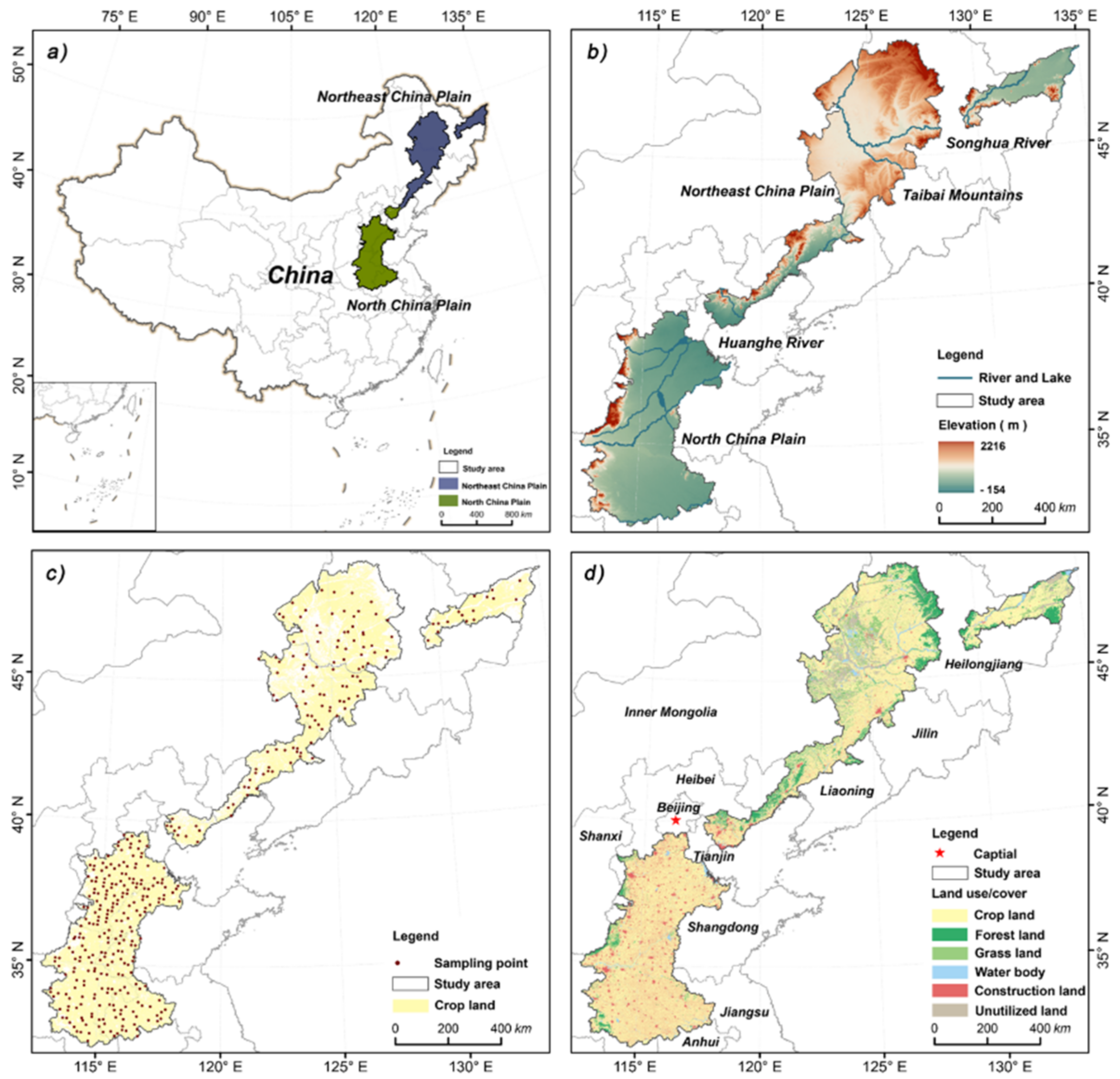
2.1. Study Area

The study area is the dryland located in the Northeast and North China Plain, covering a total area of approximately 37.79 × 10⁴ km2, including 355 counties and 7 provinces (Figure 1a). The dryland refers to the area with <5° topographic slope and >40% of the cropland area in a 1 × 1 km pixel [19]. The overall topography gradually decreases from north to south, with elevations varying from −154 to 2216 m, and the Songhua River and Yellow River flowing through the Northeast Plain and North Plain, respectively (Figure 1b). The area is dominated by a temperate continental monsoon climate. The mean annual precipitation ranges from 400 to 1200 mm, and over 70% of precipitation falls from June to August. The mean annual temperature changes by 2–16 °C from north to south. Phaeozems, chernozems, luvisols, cambisols and fluvisols are the major soil types [27]. The dryland, which is widely distributed on plains or terraces, is the dominant land-use type in the study area (Figure 1d). There are some differences in crop types between the two plains. In the Northeast Plain, the primary cultivation system is single cropping with spring wheat (Triticum aestivum), spring corn (Zea mays) and soybean (Glycine max). In contrast, double cropping is mainly used in the North Plain with summer corn and winter wheat. The study area contributes to more than 30% of national grain production, which is crucial for grain production in China.

2.2. Soil Data

The soil sampling process was established in the dryland in the Northeast and North China Plain between April and May 2017. Firstly, we overlaid DEM from the Shuttle Radar Topography Mission (SRTM) dataset [28] and land-use map in 2015 (Resource and Environment Science and Data Center, https://www.resdc.cn/, accessed on 10 Match 2017) to select dryland farming patches. Secondly, we spatially joined the maps of dryland farming patches and soil type (Institute of Soil Science, Chinese Academy of Sciences, http://www.issas.ac.cn/, accessed on 10 Match 2017). Thirdly, the settlement of sampling points was determined by the following criteria: (1) sampling points should cover all dryland farming districts and counties; (2) 5 major soil types (i.e., phaeozems, chernozem, luvisols, cambisols and vertisols) should have more than 20 sampling points; (3) sampling points should be distributed in all soil clay particle degrees (i.e., 0–5, 5–10, 10–15, 15–20, 20–25, 25–30, 30–35, 35–40, 40–45 and 45–50%). A total of 396 sampling sites (1584 samples) covered 5 kinds of soil types and 10 levels of soil clay concentration were collected (Figure 1c). For each sampling site, we collected 3 soil cores using an undisturbed soil sampler at the size of 5.1 cm diameter and 10 cm height in four depths and measured the physicochemical properties. The SOC was measured with the dichromate oxidation–external heating method [29].

2.3. Environmental Covariates

A total of 249 environmental covariates related to pedogenesis were collected [15,30] (Table S1). Environmental covariates, classified as soil and parent material, climate, organism, relief, position and remote sensing, were collected in multiple sources, including data products and indexes driven from satellites. The Landsat 8 Operational Land Imager with the 30 m spatial resolution and 16 days revisit time has been widely applicated in DSM [31]. The Landsat 8 Surface Reflectance Level 1 Tier 1, which had been operated in the process of geometric correction and radiometric correction, was used to obtain land surface reflectance information and calculate related indexes after removing the cloud and cloud shadow with the CFmask method (https://www.usgs.gov/, accessed on 21 May 2021). We composited cloudless images (a total of 2632 images) in the study area from 11 April 2013 to 1 July 2017 and then calculated the average of each band. Soil and vegetation indexes (i.e., Normalized difference vegetation index, carbonate index) were determined by band calculation. We performed principal component analysis (PCA) and tasseled cap transformation (TCT) for blue, green, red, near-infrared, shortwave infrared 1 and shortwave infrared 2 bands [32,33]. Three principal components (i.e., principal component 1, principal component 2 and principal component 3) and three tasseled cap components (i.e., tasseled cap 1, tasseled cap 2 and tasseled cap 3) were used to further extract the information in the spectral reflectance, which might not be considered in indexes.
Relief covariates were obtained from 90 m spatial resolution DEM produced by SRTM (https://srtm.csi.cgiar.org, accessed on 21 May 2021). We used SAGA GIS (http://www.saga-gis.org/, accessed on 16 June 2021) to derive 111 relief factors covering basic terrain indexes, standard flow indexes, landform class indexes, soil or hydrological deposition and accumulation indexes and climate indexes determined by relief (i.e., aspect, slope, plan curvature, total catchment area).
There were also some existing data products used to represent soil landform features. The 1 km spatial resolution WorldClim products from 1970 to 2000 contained 7 climatology variables and 14 bioclimatic variables, and we calculated the annually average values of each variable to represent climate information [34,35]. There were some variables based on MODIS data products: land surface day temperature and land surface night temperature in MOD11A1 (1 km, daily), evapotranspiration, potential evapotranspiration, latent heat flux and potential latent heat flux in MOD16A2 (1 km, 8 day), gross primary production in MOD17A2H (500 m, 8 day), net primary productivity in MOD17A3HGF (500 m, yearly), burn date and fractional tree cover in MOD44B (250 m, yearly), leaf area index and fraction of absorbed photosynthetic active radiation (FAPAR) in MOD15A2H (500 m, 8 day) (https://lpdaac.usgs.gov/, accessed on 5 July 2021). These were aggregated into yearly products from 2001 to 2017 and then calculated the average. In addition, we collected five categorical variables: soil Type (ST) [36], lithology (LI) [37], soil erosion (SE), pedoclimatic zone and vegetation type (http://www.resdc.cn, accessed on 5 July 2021). All environmental covariates were resampled to the 1 km spatial resolution using the nearest algorithm and the coordinate system was unified into the Beijing54 Albers Equal Area projection. The preprocessing of variables was performed in the Google Earth Engine [26].

2.4. Modeling Methodology

The modeling process mainly contained feature selection, model development, model validation and uncertainty assessment. The feature selection was performed in Matlab 2014 (The MathWorks Inc., Natick, MA, USA). The model development, model validation and uncertainty assessment were implemented with the caret, xgboost, randomForest, Cubist, rgdal, lattice and ggplot2 packages in R 3.6.1 [38].

2.4.1. Feature Selection

There were 249 covariates in the original dataset, with high multicollinearity and redundant information, which had negative effects on fitting and computing efficiency. We introduced the Genetic Algorithm (GA) to select informative predictive variables [39]. GA is a heuristic search algorithm that imitates Darwinian natural evolution theory to detect optimal values in groups [40]. All environmental covariates were expressed as binary codes before feature selection. Based on the best fitness of individuals, the population repeated three primary operations (i.e., selection, crossover, mutation) until reaching the stopping criteria. Three operations were mainly controlled by six main parameters (i.e., population size, max generations, convergence, mutation rate, cross validation (CV) fold, replicate runs). The result selected by the GA remained the main information of the full features and sharply reduced multicollinearity among covariates. Following prior research, we defined population size, max generations, convergence, mutation rate, CV fold and replicate runs as 60, 200, 0.6, 0.001, 10 and 100, respectively [41]. The partial least-squares regression was used as the regression model for the GA to perform feature selection. Consequently, 29 environmental covariates, including 7 soil and parent material factors, 5 climate factors, 7 organism factors, 6 relief factors and 4 remote sensing factors, were selected to fit models (Table 1).

2.4.2. Model Development

Machine learning has advantages in dealing with massive and highly multicollinear data, and has been widely used in DSM [10,42]. In this study, we compared three dominating machine learning methods algorithms based on tree models (Cubist, XGBoost, RF) in predicting SOC in four soil depths.
Based on the M5 model, Cubist is one of the regression tree algorithms [43]. Compared with the CART model, linear regression models are used in the termination of tree leaves instead of discrete variables for Cubist, thus more local linearity variable space can be captured, which leads to more a straightforward model structure and higher prediction accuracy [43,44]. The committee (the number of committee models) and the neighbor (data partition) play important roles in the model performance [45]. Based on the standard of minimal root mean square error (RMSE) in 10-fold CV, committee and neighbor were selected as 20 and 8 via the grid search method.
XGBoost is a gradient boosting tree algorithm [46]. XGBoost creates multiple interactional weak predictors and ensemble single results with a weighted summation. XGBoost randomly selects subsets to iteratively fit single predictors to obtain the minimized loss function and introduces the stochastic gradient boosting procedure, which can reduce the risk of overfitting and improve the generalization of models with regularization [16]. Seven parameters, including the learning rate (eta of 0.2), the number of iterations (nround of 150), the max depth of a single tree (max depth of 4), the decrease of the minimum loss function required for node splitting (gamma of 0.001), the number of attributes used in single tree (colsample bytree of 0.5), the sample weight sum of minimum leaf node (min child weight of 3) and the rate of random sampling for single tree (subsample of 0.8), were defined to control the single tree change and the iteration process.
RF is a bagging ensemble learning algorithm [47]. RF creates many decision trees as predictors, and calibration samples and feature collections are randomly selected to fit each predictor. As the overall predicted result is the average of every decision tree, RF is less affected by outliers and has a relatively stable performance. There are two key parameters in the RF model: the number of trees (ntree of 500) and the number of variable features in the spilt of the binary tree (mtry of 13) [48].

2.4.3. Model Validation

The whole soil dataset (386 sites) was divided into the calibration dataset (80%, 306 sites) and the validation dataset (20%, 80 sites). For each predictive model, we calculated two evaluating indices: coefficient of determination (R2) and RMSE. The values of indices were the average of 50 iterations, and the equations were as follows:
R 2 = 1 i = 1 n y i y p 2 i = 1 n y i y a 2
R M S E = 1 n i = 1 n y i y p 2
where n is the number of sampling points, y i and y p are the measured and predicted values for sample i and y a is the average of the measured values.

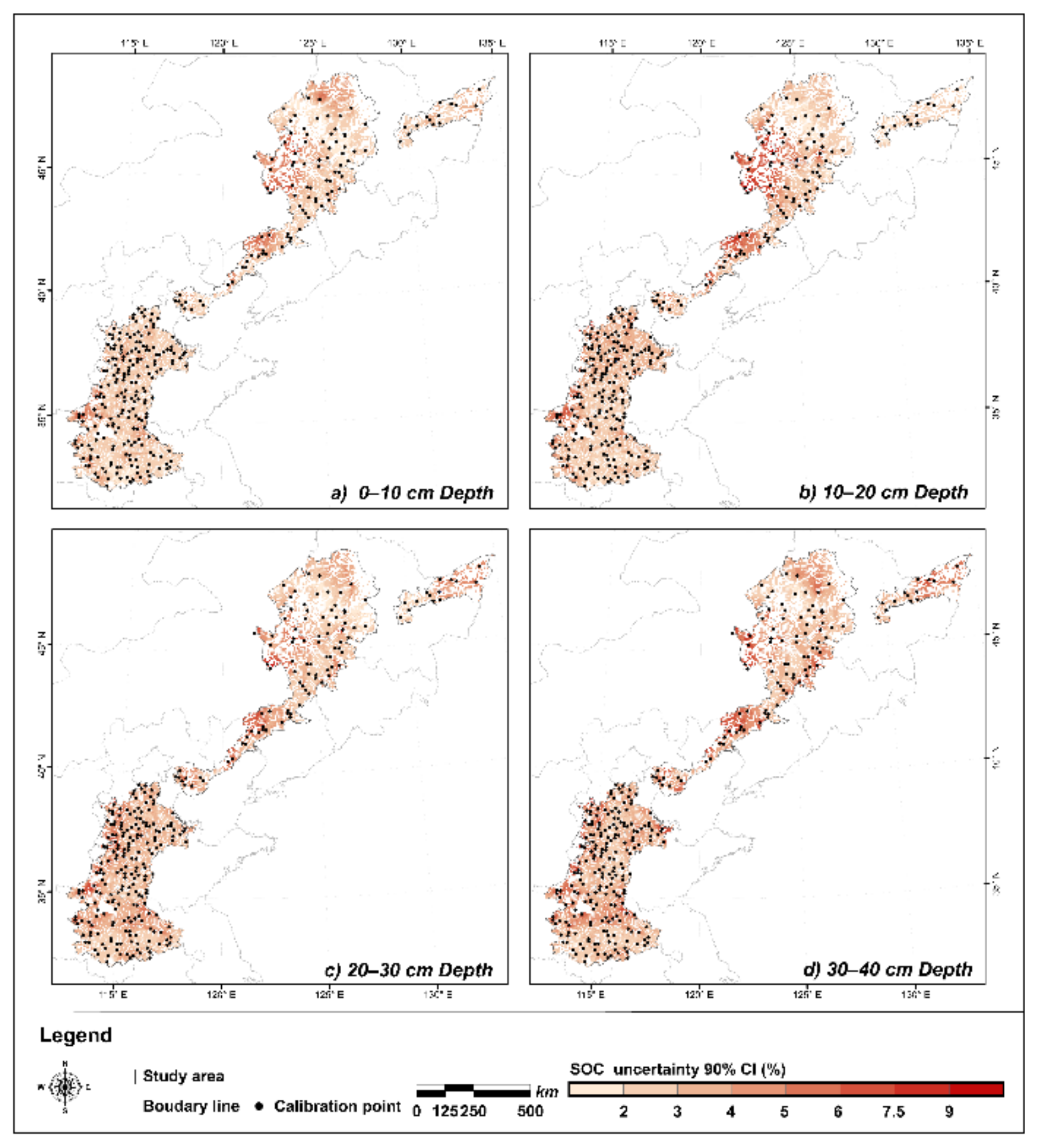
2.4.4. Uncertainty Assessment

As random sampling generated errors in machine learning algorithms, we applied a nonparametric statistical method called bootstrap to estimate the uncertainty of the predictions. The bootstrap is one of the repeated sampling methods which randomly selects samples with replacement. The new bootstrapped dataset and original dataset have the same sample number and a similar probability distribution. We generated 50 bootstrapped datasets for calibration datasets in each depth. The average accuracy in validation datasets and the average prediction of the SOC were considered as the final assessment indicator and the predicted result, respectively. We calculated the possible changing ranges of the actual values in each pixel by the confidence interval (CI) at the 90% level (Equation (3)). The uncertainty could be finally calculated in Equation (4):
C I = P a ± c × S D N
U = C I u p p e r C I l o w e r P a × 100
where C I is the 90% confidence interval, P a is the average predicted result of each model in all rounds, c is the coefficient related to the confidence interval level and iterations, S D is the standard deviation of all the predictions, N is the number of iterations, U represents the uncertainty and C I u p p e r and C I l o w e r represent the upper and lower 90% confidence limits.

3. Results

3.1. Descriptive Statistics for SOC

The statistics of SOC in 386 sampling points are shown in Table 2 and Figure 2. The mean SOC concentration decreased with deepening depth and the mean value was 9.16 g kg−1 in the 0–40 cm depth. The standard deviations (SD) of the SOC were 4.86, 4.98, 4.53 and 4.17 g kg−1, respectively, and the variations of the SOC in the four soil depths were high, with the coefficient of variation of 38.66, 49.22, 59.79 and 65.46% [49]. The original sampling of SOC data in the four depths presented positive skewness distribution (0.71, 1.37, 1.42 and 1.52) (Table 2). The kurtosis values were 3.80, 5.01, 4.83 and 4.89, respectively, which showed the SOC concentration in the first layer was closer to the normal distribution. Though the Kolmogorov–Smirnov test showed soil data for each depth slightly deviated from normality, it did not have negative effects on modeling process, as machine learning algorithms do not rely on the data contribution amusement [50].

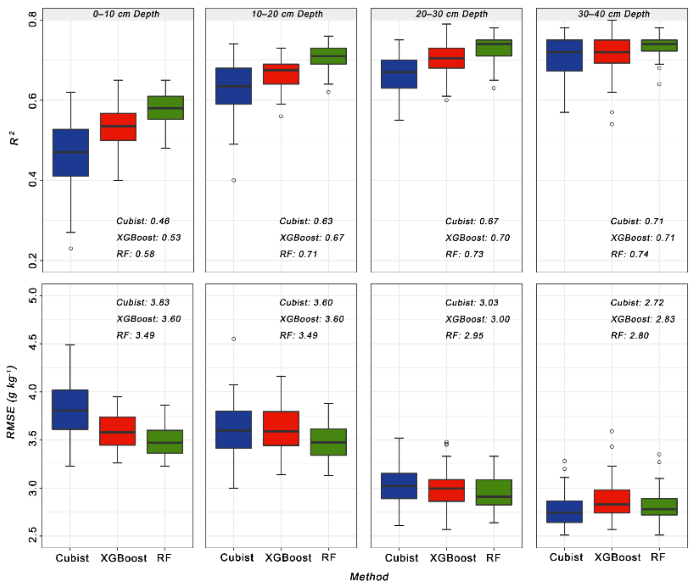
3.2. Model Evaluation and Comparison

The average values of the two evaluating indices (i.e., R2, RMSE) in the validation dataset through 50 bootstrap rounds were selected to estimate the model accuracy (Table 3 and Figure 3). Meanwhile, we calculated the relative RMSE (RRMSE) by dividing the RMSE by the mean measured values in order to eliminate dimensional effects. Compared with XGBoost and Cubist, RF performed better in four soil depths (Table 3, Figure 3). The R2 represents the explanatory ability of the prediction results to the measured values. Our results showed the R2 of RF was 0.58 (0–10 cm depth), 0.71 (10–20 cm depth), 0.73 (20–30 cm depth) and 0.74 (30–40 cm depth), which was 0.05, 0.04, 0.03 and 0.03 higher than XGBoost and 0.12, 0.08, 0.06 and 0.03 higher than Cubist. We found there was an obvious improvement in the top two depths and the difference in accuracy in the three models decreased with the depths. Meanwhile, we found that three models all performed better in deep soil depths. For example, the RMSE of RF decreased with increasing depths, with 3.49, 3.49, 2.95 and 2.80 g kg−1 in four depths.
The uncertainty results for the validation data in the four soil depths with Cubist, XGBoost and RF are shown in Figure 4. Compared with Cubist and XGBoost, RF still had the lowest uncertainty (Figure 4). While different from model accuracy indices, the uncertainty was higher in the deep soil depths as the mean measured values were lower. For example, the average uncertainty values of RF in four soil depths were 3.10, 3.17, 3.75 and 3.96%, which were consistent with the RRMSE values (0.29, 0.34, 0.38 and 0.43 in the four depths). We subsequently analyzed the relationship between the measured values and the predicted values and found the high SOC was underestimated and the low SOC was overestimated by three models. The average values of the absolute residual in the predicted values were 3.25 (Cubist), 2.89 (XGBoost) and 3.09 (RF) in low measured values (below 10 g kg−1); 1.99 (Cubist), 1.71 (XGBoost) and 1.70 (RF) in median measured values (range from 10 to 20 g kg−1); 7.19 (Cubist), 7.68 (XGBoost) and 7.21 (RF) in high measured values (above 20 g kg−1), which also proved there was less deviation in the middle SOC concentration (Figure 4).

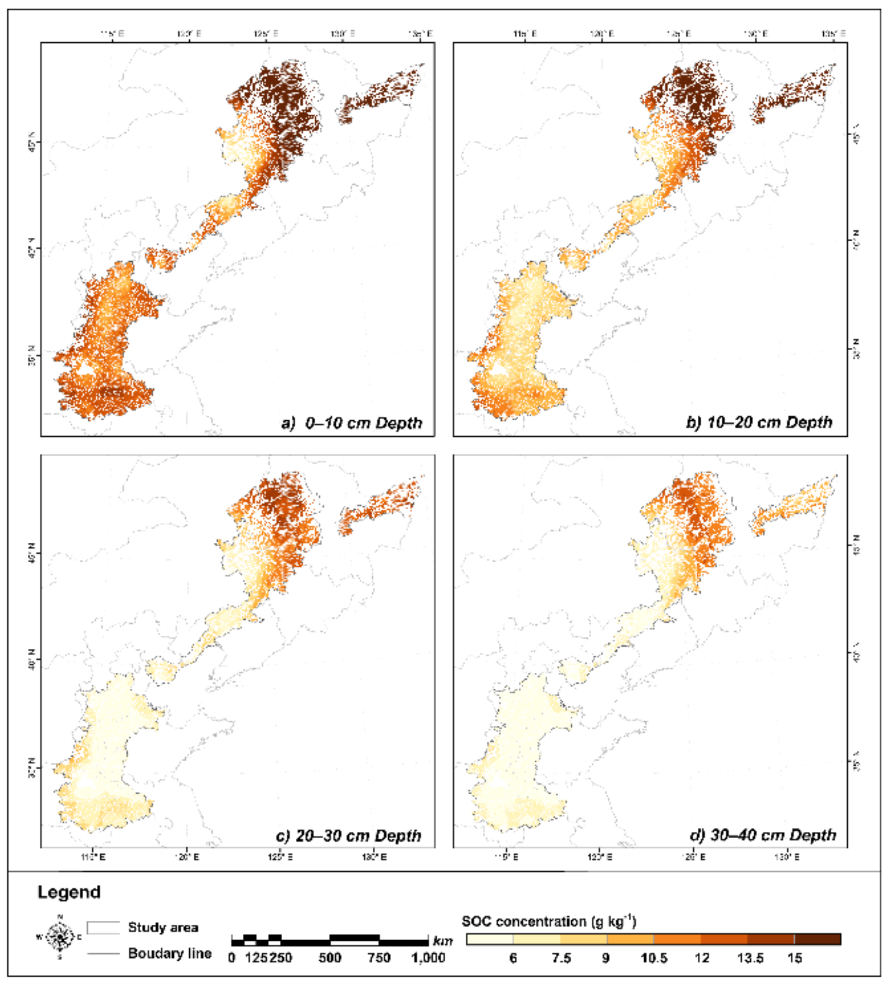
3.3. Spatial Distribution Pattern of SOC

The spatial distribution patterns of SOC in different soil depths were similar for Cubist, XGBoost and RF (Figure 5 and Figure S1). The predictions of RF, which possessed the optimal accuracy and minimal uncertainty, could precisely represent regional SOC and were finally chosen to explain the distribution patterns of SOC (Figure 5). The average values of SOC decreased with the depth and the average values in 0–10, 10–20, 20–30 and 30–40 cm were 13.21, 10.85, 8.26 and 7.08 g kg−1, respectively. Compared with the North Plain, SOC was higher in the Northeast Plain in the four soil depths. In the 0–10 cm soil depth, the average SOC was 11.96 g kg−1 in the North Plain, while it was 14.68 g kg−1 in the Northeast Plain. In the 10–20 cm soil depth, the average SOC was 8.96 g kg−1 in the North Plain, while it was 13.07 g kg−1 in the Northeast Plain. In the 20–30 cm soil depth, the average SOC was 6.12 g kg−1 in the North Plain, while it was 10.81 g kg−1 in the Northeast Plain. In the 30–40 cm soil depth, the average SOC was 5.06 g kg−1 in the North Plain, while it was 9.47 g kg−1 in the Northeast Plain. Regarding the spatial distribution pattern, the SOC significantly increased with latitudes in the Northeast Plain, while there was higher SOC in the margin of the North Plain, especially in the south, west and northeast area. Despite this, the region overall showed a relatively stationary distribution, with a SD of 1.15, 1.38, 1.20 and 1.01 in the four soil depths. Overall, the SOC increased from south to north in the study area and gradually decreased with increasing depth.

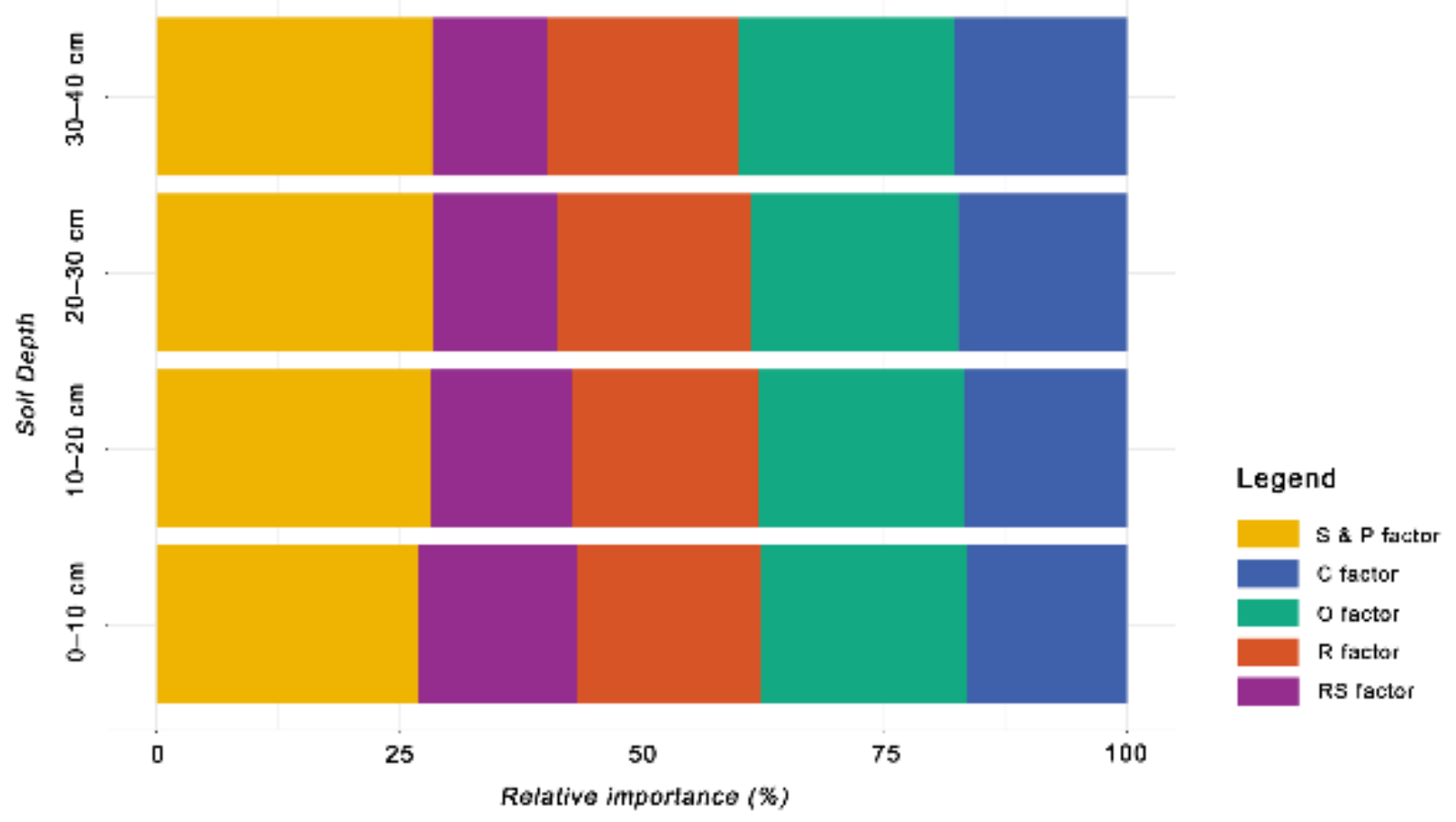
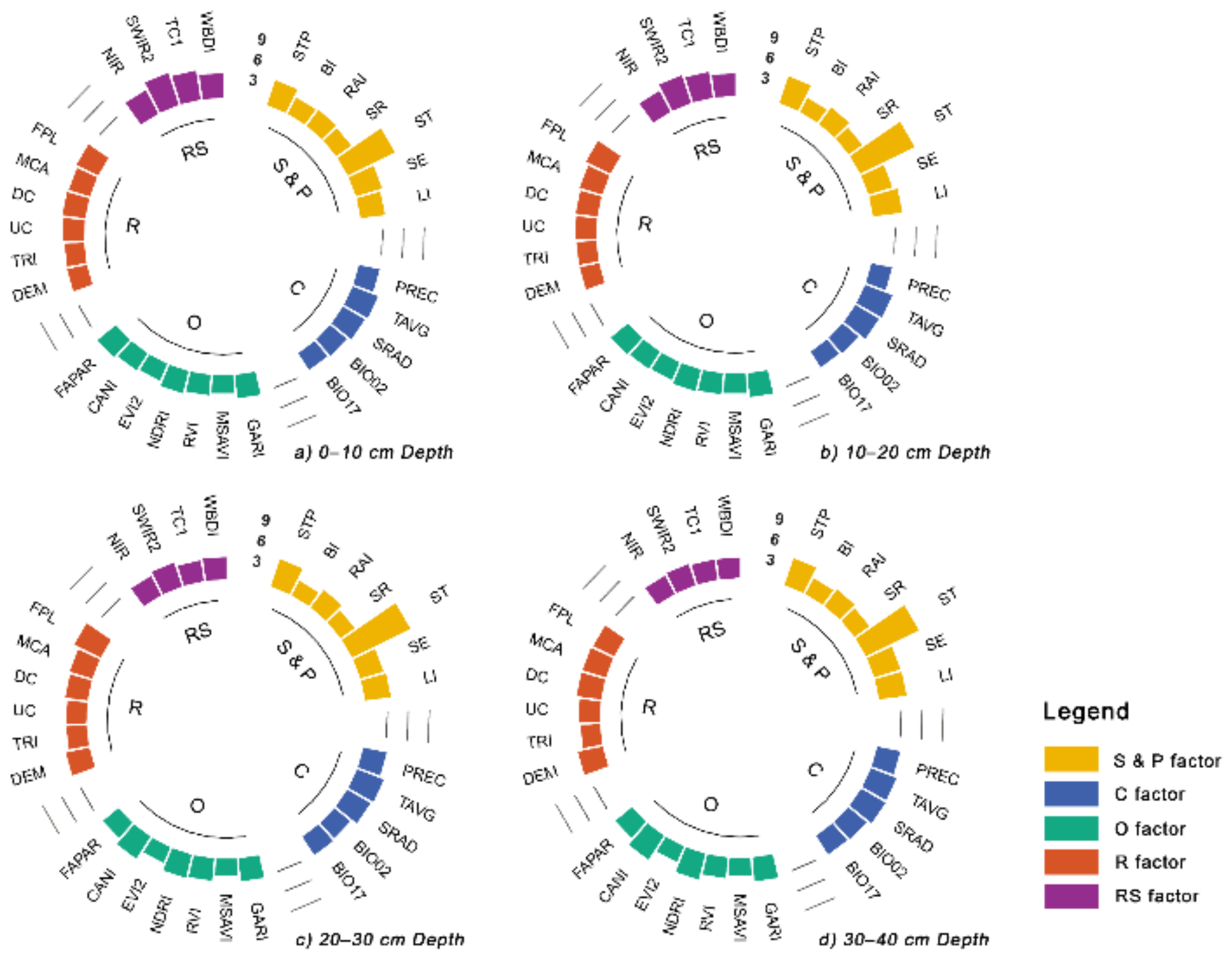
3.4. Relative Importance of Environmental Covariates

The importance of covariates could be calculated by the increasing mean error of trees in the progress of model fitting. The importance of environmental covariates in RF is shown in Figure 6. The soil and parent material with percentages of 26.96, 28.23, 28.47 and 28.42% in the four soil depths was the primary impact factor, followed by the organism (21.23, 21.35, 21.35 and 22.25%), the relief (18.77, 19.07, 19.94 and 19.63%) and the climate (16.58, 16.74, 17.40 and 17.79%). The importance of the soil and parent material and the relief increased in the first three depths, while it slightly decreased in the 30–40 cm soil depth. Meanwhile, the importance of the organism and the climate showed a relatively stable tendency, while the remote sensing band reflectance and derivative contributed minimally, and decreased with the depth getting deeper (16.46, 14.61, 12.84 and 11.90% in the four soil depths).
The proportion of the detailed environmental covariates in the factors is shown in Figure 7. We found that the contribution rates of the major environmental covariates in the four soil depths changed slightly. The ST played a vital role in the soil and parent material, with an average contribution rate of 8.49, followed by soil temperature (STP, 3.99), LI (3.85), SE (3.72), reflectance absorption index (RAI, 2.98), stress-related (SR, 2.52) and brightness index (BI, 2.46). The average contribution rates of mean temperature (TAVG), solar radiation (SRAD), mean precipitation (PREC), mean diurnal range (BIO02) and precipitation of driest quarter (BIO17) were similar, with the values of 4.02, 3.86, 3.19, 3.09 and 2.96, respectively. As for the organism factor, the difference in the average contribution rates of the covariates was slight, with the average value of 2.56 (EVI2: two-band enhanced vegetation index), 2.60 (MSAVI: modified soil-adjusted vegetation index), 3.02 (RVI: ratio vegetation index), 3.13 (FAPAR), 3.38 (GARI: green atmospherically resistant vegetation index), 3.42 (CANI: canopy index) and 3.43 (NDRI: normalized difference red/green redness index). The subrelief factors were of almost equal importance (average contribution rates of 3.19, 2.76, 2.98, 3.50, 3.47 and 3.30 in elevation (DEM), terrain ruggedness index (TRI), upslope curvature (UC), downslope curvature (DC), modified catchment area (MCA) and flow path length (FPL), respectively). The shortwave infrared 2 band reflectance (SWIR2) was the foremost remote sensing factor, although it decreased in the deep soils (4.86 in 0–10 cm, 3.17 in 30–40 cm). The average contribution rates of the near-infrared band reflectance (NIR), tasseled cap 1 (TC1) and the wetness brightness difference index (WBDI) were almost equal (3.32, 3.47 and 3.20, respectively). Overall, the soil and parent material was the dominant factor in the spatial predictions of regional SOC, followed by the organism, relief, climate and remote sensing factor. Although there were differences in the four soil depths, the ST, TAVG, CANI, FPL and SWIR2 were the pivotal five factors.

4. Discussion

4.1. Model Performance

Compared with Cubist and XGBoost, RF showed the optimal prediction performance in the 50 rounds of bootstrap, which was consistent with many studies [16,51], while RF was prone to predicting conservatively, and there was some deviation in the outliers. That is because the prediction result is from the average of the independent predictors, which promotes the antinoise ability of the models but decreases the sensitivity of extremums [47]. As for the boosting models, the residuals from the former predictors are used to fit the subsequent models, which can repeatedly adjust the model but increases the risk of overfitting [46]. As shown in our study, SOC was slightly underestimated in the north and overestimated in the south.
Our result indicated an increasing tendency of the model performance with the depth getting deeper in the soil tillage layer. The average R2 of the SOC prediction on a broadscale DSM was 0.49 (0–30 cm), 0.28 (30–100 cm) and 0.14 (100–200 cm), summarized from 126 articles between 2003 and 2021 [4]. We obtained the average R2 of 0.58, 0.71, 0.73 and 0.74 and the RMSE of 3.49, 3.49, 2.95 and 2.80 g kg−1 with the RF models in four depths, showing our results were better than almost all studies, which proved the sampling design was relatively reasonable and that the relationships between the regional SOC and environment were fully captured. Thus, it is an effective way to quantify the spatio-temporal information in environmental covariates with cloud computing platforms, which can help improve the model performance in future DSM work. Moreover, the criteria can provide the reference in sampling design at large scales in other areas of the world. The environmental covariate system can be also introduced in DSM studies in the Northeast and North Plain China.
The increase of the model accuracy with deepening depths was consistent with previous studies [51,52]. Gomes, et al. [51] reported that the performance of the RF models in predicting Brazil SOC stocks increased in 0–5, 5–15, 15–30 and 30–60 cm soil depths but decreased in the 60–100 cm depth. Liu, et al. [52] drew the same conclusions when modeling the SOC in China. As our study focused on the tillage layers with a relatively close interval, there was less variability of the SOC in the four depths. Moreover, compared with the topsoil, there was a less human disturbance in the deeper depth and the environmental covariates can better explain the SOC distribution, which may offset the negative effect of higher variability for model fitness [31]. Thus, the model performed better in the deeper depth.

4.2. Spatial Distribution Pattern of SOC and Controlling Factors

Our study showed that SOC overall increased from south to north and decreased with increasing depth, which was related to soil and environmental factors. The spatial variability in the study area was controlled by environmental variables [53]. Our results showed that soil and parent material played a dominant role in model fitness and influenced more with increasing depths (26.96, 28.23, 28.47 and 28.42% in the four soil depths), which was consistent with numerous studies in large scales [18,54]. Subsequently, ST was the major subfactor in the group. That is because the soil type is the comprehensive reflection of climate, relief and parent material, which can represent the potential soil carbon and can be considered as an important SOC indicator on large scales [55]. Our study area covered approximately 22 degree longitudes and 17 degree latitudes, including 20 main soil types, causing significant differences in the initial element concentration and soil mineralization levels, which determined the general SOC distribution patterns in the area [56]. Organism was the second important factor, and the relative importance was similar in the four depths (21.23, 21.34, 21.35 and 22.25%). As our study focused on croplands, multiple management measures led to great differences in vegetation variety and productivity, tillage rotation, fertilizer utilization, soil erosion, etc., which influenced the attainable SOC [54,57]. We used the long-term averages of vegetation indexes (e.g., GARI, NDRI, CANI) and FAPAR to explain the vegetation coverage and growth conditions, vegetation productivity and photosynthetic intensity. We did not find a pronounced decrease in the contribution rates with the increase in soil depths. It may be because there is only 10 cm between each soil depth and they all belong to tillage layers, where the organism distribution is relatively continuous. As our study area was distributed in croplands with a <5° slope and 100–200 m altitude in the Northeast and North China Plain, terrain conditions were relatively consistent, which was not enough to make an obvious difference in heat accumulation, precipitation distribution and surface runoff [58]. We found TAVG and SRAD were the main subclimate factors, which was consistent with several recent studies [59,60]. That is because the increasing temperature can have a positive effect on soil biota activities, and this subsequently accelerates the oxidation process of soil carbon [61]. Meanwhile, solar radiation can positively influence vegetation growth but negatively change surface evaporation [60]. As our study area is drylands in the plain with a relatively moderate climate, there is less variation of vegetation growth caused by the difference in solar radiation, while high solar radiation limits microbial activities and decreases SOC [62].
Overall, our study indicated that though long-term cultivation made disturbance in soils, the spatial distribution pattern of the SOC generally can be better explained by the environmental covariates. Moreover, in the relatively large region, the soil and parent material and organism were the most important covariates in the SOC prediction, which should be fully considered and quantified when mapping SOC in the large scale.

4.3. Digital SOC Mapping and Its Uncertainty

We applied bootstrap to quantify the spatial distribution pattern of prediction uncertainty [63]. The uncertainty of predictions is shown in Figure 8 and Figure S2, and the potential causes can be summarized into two aspects.
Firstly, the uncertainty originates from the sampling density. Our study found higher uncertainty in the area with relatively scattered fields, high elevation and few sampling sites. This was due to lacking information on the relationships between the soil and environmental covariates. In the deep soil depths, the uncertainty was slightly higher. This was because the average SOC concentration was low in the deeper soil depth, and thus it was more sensitive to the predicted deviations, causing little higher uncertainty. More detailed soil information can be collected by increasing the regional sampling density. Meanwhile, the spatial variability of the environmental covariates can be captured more precisely, which greatly contributes to decreasing the deviation of the sampling points, especially in the dramatic change area of environment and soil properties [64].
Secondly, the uncertainty derives from the quantity and quality of the environmental covariates. Although we collected as many environmental covariates as possible, there were some unavailable and unquantified factors [9]. Some studies introduced gamma radiometric and categorical geology variables to improve model performance [56,65], while these covariates are unavailable in the study area, which may lead to the lack of information on geology, and finally have negative effects on uncertainty. In addition, we used data products in multiple sources and translated them into the same spatial resolution by downscaling or upscaling methods, and the error in the data products and calculations may be propagated into the predictions.
Overall, the uncertainty can be controlled by increasing the sampling density, capturing informative covariates and optimizing the spatial modeling methods. With high-quality sampling data and environmental covariates, the uncertainty in the process of sampling and modeling can be minimized, especially in the area with the rapid change of soils and landscape, which can contribute to improving the reliability and accuracy of the data products.

4.4. Limitations and Perspectives

Our study updated the dryland SOC map in the Northeast and North Plain China based on optimal covariates and models, but limitations should be addressed later.
Firstly, the spatio-temporal variation information of the environmental covariates needs to be sufficiently quantified. We considered commonly used environmental covariates to fit the prediction models and generate reliable results. However, pedogenesis is an extraordinarily complicated and long-term interaction between the parent material and environment, and thus we need to quantify further the effects of pedogenesis factors and human activities [66]. Meanwhile, global and regional DSM studies have dramatically appeared in recent years, and thus it might be a good strategy to utilize previous products and legacy data to update products and improve the accuracy and stability of predictions [67,68].
Secondly, it is essential to map multiperiod cropland SOC stock products. Previous studies have proved that SOC changed dramatically in land use and cover change [69]. Besides our study, there have been considerable SOC/SOM studies with the DSM framework since 2003, while the number of SOC stock studies is relatively low [4]. The SOC stock directly quantify regional carbon storage, determining the SOC baselines and variable amounts in the different periods [70]. Meanwhile, there is an increasing demand for multiperiod DSM products to support the research of precision agriculture and ecosystem change [4,15]. Towards this, further studies need to focus on mapping multiperiod cropland SOC with sampling points in a relatively unified distribution.

5. Conclusions

This study compared three machine learning algorithms based on tree models and estimated the spatial distribution patterns of the dryland SOC in the Northeast and North Plain China. This study revealed the spatial distribution of dryland SOC in the Northeast and North China Plain with informative environmental covariates and optimal models. The following conclusions can be summarized:
  • Compared with XGBoost and Cubist, RF was the optimal model for predicting regional SOC, with the highest accuracy and the lowest uncertainty.
  • The SOC overall increased from south to north and decreased with increasing depth. In the North Plain, the SOC was higher in the margin, while it increased with latitude in the Northeast Plain, with high values in the typical black soil region.
  • The spatial variation was mainly influenced by the soil and parent material, organism, relief and climate.
The results updated the regional dryland SOC maps and indicated the potential causes of the prediction uncertainty, which could help evaluate soil quality dynamics after long-term cultivation and guide subsequent high-resolution DSM research. Meanwhile, the sampling and the environmental covariate database can provide reliable reference for mapping SOC in other areas of the world.

Supplementary Materials

The following supporting information can be downloaded at: https://www.mdpi.com/article/10.3390/rs14102504/s1, Figure S1. Spatial and vertical distribution pattern of SOC concentration with Cubist, XGBoost and RF; Figure S2. Spatial and vertical distribution pattern of uncertainty with Cubist, XGBoost and RF; Table S1. List of all environmental covariates.

Author Contributions

Conceptualization, X.Z., Z.Z. and Z.S.; methodology, X.Z., S.C. and Z.S.; software, X.Z. and J.X.; validation, X.Z. and Y.H.; formal analysis, X.Z. and N.W.; investigation, X.Z., Z.Z. and Y.H.; writing—original draft preparation, X.Z. and Z.Z.; writing—review and editing, X.Z., Z.S. and S.C.; visualization, X.Z. and J.X.; supervision, Z.Z. and Z.S.; funding acquisition, Z.S. and Y.H. All authors have read and agreed to the published version of the manuscript.

Funding

This research was funded by the National Key Research and Development Program (2018YFE0107000), Ten-thousand Talents Plan of Zhejiang Province (2019R52004), the National Key R&D Program of China (2021YFD1500201) and the China Postdoctoral Science Foundation (2021M702840). The authors are deeply grateful to the anonymous reviewers and the editor for their helpful comments on the manuscript.

Institutional Review Board Statement

Not applicable.

Informed Consent Statement

Not applicable.

Data Availability Statement

Not applicable.

Conflicts of Interest

The authors declare no conflict of interest.

References

  1. Owusu, S.; Yigini, Y.; Olmedo, G.F.; Omuto, C.T. Spatial prediction of soil organic carbon stocks in Ghana using legacy data. Geoderma 2020, 360, 114008. [Google Scholar] [CrossRef]
  2. Houghton, J.T.; Ding, Y.; Griggs, D.J.; Noguer, M.; van der Linden, P.J.; Dai, X.; Maskell, K.; Johnson, C. Climate Change 2001: The Scientific Basis; Cambridge University Press: New York, NY, USA, 2001. [Google Scholar]
  3. Lal, R. Soil carbon sequestration impacts on global climate change and food security. Science 2004, 304, 1623–1627. [Google Scholar] [CrossRef] [PubMed] [Green Version]
  4. Chen, S.; Arrouays, D.; Leatitia Mulder, V.; Poggio, L.; Minasny, B.; Roudier, P.; Libohova, Z.; Lagacherie, P.; Shi, Z.; Hannam, J.; et al. Digital mapping of GlobalSoilMap soil properties at a broad scale: A review. Geoderma 2022, 409, 115567. [Google Scholar] [CrossRef]
  5. Goldstein, A.; Turner, W.R.; Spawn, S.A.; Anderson-Teixeira, K.J.; Cook-Patton, S.; Fargione, J.; Gibbs, H.K.; Griscom, B.; Hewson, J.H.; Howard, J.F.; et al. Protecting irrecoverable carbon in Earth’s ecosystems. Nat. Clim. Change 2020, 10, 287–295. [Google Scholar] [CrossRef]
  6. Paustian, K.; Lehmann, J.; Ogle, S.; Reay, D.; Robertson, G.P.; Smith, P. Climate-smart soils. Nature 2016, 532, 49–57. [Google Scholar] [CrossRef] [PubMed] [Green Version]
  7. Zeraatpisheh, M.; Ayoubi, S.; Mirbagheri, Z.; Mosaddeghi, M.R.; Xu, M. Spatial prediction of soil aggregate stability and soil organic carbon in aggregate fractions using machine learning algorithms and environmental variables. Geoderma Reg. 2021, 27, e00440. [Google Scholar] [CrossRef]
  8. Tubiello, F.N.; Salvatore, M.; Ferrara, A.F.; House, J.; Federici, S.; Rossi, S.; Biancalani, R.; Condor Golec, R.D.; Jacobs, H.; Flammini, A.; et al. The Contribution of Agriculture, Forestry and other Land Use activities to Global Warming, 1990–2012. Glob. Chang Biol. 2015, 21, 2655–2660. [Google Scholar] [CrossRef] [Green Version]
  9. Lagacherie, P.; McBratney, A. Spatial soil information systems and spatial soil inference systems: Perspectives for digital soil mapping. Dev. Soil Sci. 2006, 31, 3–22. [Google Scholar] [CrossRef]
  10. Chen, S.; Martin, M.P.; Saby, N.P.A.; Walter, C.; Angers, D.A.; Arrouays, D. Fine resolution map of top-and subsoil carbon sequestration potential in France. Sci. Total Environ. 2018, 630, 389–400. [Google Scholar] [CrossRef]
  11. Zeraatpisheh, M.; Bakhshandeh, E.; Hosseini, M.; Alavi, S.M. Assessing the effects of deforestation and intensive agriculture on the soil quality through digital soil mapping. Geoderma 2020, 363, 114139. [Google Scholar] [CrossRef]
  12. Zhang, G.; Liu, F.; Song, X. Recent progress and future prospect of digital soil mapping: A review. J. Integr. Agric. 2017, 16, 2871–2885. [Google Scholar] [CrossRef]
  13. Hong, Y.; Chen, S.; Chen, Y.; Linderman, M.; Mouazen, A.M.; Liu, Y.; Guo, L.; Yu, L.; Liu, Y.; Cheng, H.; et al. Comparing laboratory and airborne hyperspectral data for the estimation and mapping of topsoil organic carbon: Feature selection coupled with random forest. Soil Tillage Res. 2020, 199, 104589. [Google Scholar] [CrossRef]
  14. Taghizadeh-Mehrjardi, R.; Khademi, H.; Khayamim, F.; Zeraatpisheh, M.; Heung, B.; Scholten, T. A Comparison of Model Averaging Techniques to Predict the Spatial Distribution of Soil Properties. Remote Sens. 2022, 14, 472. [Google Scholar] [CrossRef]
  15. Lamichhane, S.; Kumar, L.; Wilson, B. Digital soil mapping algorithms and covariates for soil organic carbon mapping and their implications: A review. Geoderma 2019, 352, 395–413. [Google Scholar] [CrossRef]
  16. Zhou, Y.; Xue, J.; Chen, S.; Zhou, Y.; Liang, Z.; Wang, N.; Shi, Z. Fine-resolution mapping of soil total nitrogen across China based on weighted model averaging. Remote Sens. 2020, 12, 85. [Google Scholar] [CrossRef] [Green Version]
  17. Ma, Y.X.; Minasny, B.; Malone, B.P.; Mcbratney, A.B. Pedology and digital soil mapping (DSM). Eur. J. Soil Sci. 2019, 70, 216–235. [Google Scholar] [CrossRef]
  18. Chen, S.; Arrouays, D.; Angers, D.A.; Chenu, C.; Barre, P.; Martin, M.P.; Saby, N.P.A.; Walter, C. National estimation of soil organic carbon storage potential for arable soils: A data-driven approach coupled with carbon-landscape zones. Sci. Total Environ. 2019, 666, 355–367. [Google Scholar] [CrossRef]
  19. Zhuo, Z.; Chen, Q.; Zhang, X.; Chen, S.; Gou, Y.; Sun, Z.; Huang, Y.; Shi, Z. Soil organic carbon storage, distribution, and influencing factors at different depths in the dryland farming regions of Northeast and North China. Catena 2022, 210, 105934. [Google Scholar] [CrossRef]
  20. Chen, Q.; Shi, Z.; Chen, S.; Gou, Y.; Zhuo, Z. Role of Environment Variables in Spatial Distribution of Soil C, N, P Ecological Stoichiometry in the Typical Black Soil Region of Northeast China. Sustainability 2022, 14, 2636. [Google Scholar] [CrossRef]
  21. Zhou, Y.; Hartemink, A.E.; Shi, Z.; Liang, Z.; Lu, Y. Land use and climate change effects on soil organic carbon in North and Northeast China. Sci. Total Environ. 2019, 647, 1230–1238. [Google Scholar] [CrossRef]
  22. Tang, H.; Liu, Y.; Li, X.; Muhammad, A.; Huang, G. Carbon sequestration of cropland and paddy soils in China: Potential, driving factors, and mechanisms. Greenh. Gases Sci. Technol. 2019, 9, 872–885. [Google Scholar] [CrossRef]
  23. Yao, Y.; Tang, H.; Tang, P.; Yu, S.; Wang, D.; Si, H.; Chen, Y.; He, Y. Soil organic matter spatial distribution change over the past 20 years and its causes in Northeast. In Proceedings of the 2013 Second International Conference on Agro-Geoinformatics (Agro-Geoinformatics), Fairfax, VA, USA, 12–16 August 2013; pp. 433–438. [Google Scholar]
  24. Zhuo, Z.; Xing, A.; Cao, M.; Li, Y.; Zhao, Y.; Guo, X.; Huang, Y. Identifying the position of the compacted layer by measuring soil penetration resistance in a dryland farming region in Northeast China. Soil Use Manag. 2020, 36, 494–506. [Google Scholar] [CrossRef]
  25. Lessmann, M.; Ros, G.H.; Young, M.D.; de Vries, W. Global variation in soil carbon sequestration potential through improved cropland management. Glob. Change Biol. 2022, 28, 1162–1177. [Google Scholar] [CrossRef] [PubMed]
  26. Gorelick, N.; Hancher, M.; Dixon, M.; Ilyushchenko, S.; Thau, D.; Moore, R. Google Earth Engine: Planetary-scale geospatial analysis for everyone. Remote Sens. Environ. 2017, 202, 18–27. [Google Scholar] [CrossRef]
  27. IUSS Working Group WRB. World Reference Base for Soil Resources 2014, Update 2015 International Soil Classification System for Naming Soils and Creating Legends for Soil Maps; Food and Agriculture Organization of the United Nations: Rome, Italy, 2015. [Google Scholar]
  28. Jarvis, A.; Reuter, H.I.; Nelson, A.; Guevara, E. Hole-Filled SRTM for the Globe Version 4. CGIAR-CSI SRTM 90m Database. Available online: http://srtm.csi.cgiar.org (accessed on 9 November 2018).
  29. Bao, S. Soil Agro-Chemistrical Analysis; China Agriculture Press: Beijing, China, 2000; Volume 2030, pp. 30–107. [Google Scholar]
  30. McBratney, A.B.; Santos, M.L.M.; Minasny, B. On digital soil mapping. Geoderma 2003, 117, 3–52. [Google Scholar] [CrossRef]
  31. Liu, F.; Zhang, G.L.; Song, X.D.; Li, D.C.; Zhao, Y.G.; Yang, J.L.; Wu, H.Y.; Yang, F. High-resolution and three-dimensional mapping of soil texture of China. Geoderma 2020, 361, 114061. [Google Scholar] [CrossRef]
  32. Wold, S.; Esbensen, K.; Geladi, P. Principal component analysis. Chemom. Intell. Lab. Syst. 1987, 2, 37–52. [Google Scholar] [CrossRef]
  33. Crist, E.P.; Cicone, R.C. A Physically-Based Transformation of Thematic Mapper Data—The Tm Tasseled Cap. IEEE Trans. Geosci. Remote Sens. 1984, 22, 256–263. [Google Scholar] [CrossRef]
  34. Fick, S.E.; Hijmans, R.J. WorldClim 2: New 1-km spatial resolution climate surfaces for global land areas. Int. J. Climatol. 2017, 37, 4302–4315. [Google Scholar] [CrossRef]
  35. Hijmans, R.J.; Cameron, S.E.; Parra, J.L.; Jones, P.G.; Jarvis, A. Very high resolution interpolated climate surfaces for global land areas. Int. J. Climatol. 2005, 25, 1965–1978. [Google Scholar] [CrossRef]
  36. Fischer, G.; Nachtergaele, F.; Prieler, S.; van Velthuizen, H.; Verelst, L.; Wiberg, D. Global Agro-Ecological Zones Assessment for Agriculture (GAEZ 2008); IIASA: Laxenburg, Austria; FAO: Rome, Italy, 2008; Volume 10. [Google Scholar]
  37. Hartmann, J.; Moosdorf, N. The new global lithological map database GLiM: A representation of rock properties at the Earth surface. Geochem. Geophy. Geosystems 2012, 13, 1–37. [Google Scholar] [CrossRef]
  38. R Core Team. R: A Language and Environment for Statistical Computing; R Foundation for Statistical Computing: Vienna, Austria, 2021. [Google Scholar]
  39. Taghizadeh-Mehrjardi, R.; Nabiollahi, K.; Kerry, R. Digital mapping of soil organic carbon at multiple depths using different data mining techniques in Baneh region, Iran. Geoderma 2016, 266, 98–110. [Google Scholar] [CrossRef]
  40. Holland, J.H. Adaptation in Natural and Artificial Systems: An Introductory Analysis with Applications to Biology, Control, and Artificial Intelligence; MIT Press: Cambridge, MA, USA, 1992. [Google Scholar]
  41. Welikala, R.A.; Fraz, M.M.; Dehmeshki, J.; Hoppe, A.; Tah, V.; Mann, S.; Williamson, T.H.; Barman, S.A. Genetic algorithm based feature selection combined with dual classification for the automated detection of proliferative diabetic retinopathy. Comput. Med. Imaging Graph. 2015, 43, 64–77. [Google Scholar] [CrossRef] [PubMed] [Green Version]
  42. Wadoux, A.M.J.C.; Minasny, B.; McBratney, A.B. Machine learning for digital soil mapping: Applications, challenges and suggested solutions. Earth-Sci. Rev. 2020, 210, 103359. [Google Scholar] [CrossRef]
  43. Quinlan, J.R. Combining instance-based and model-based learning. In Proceedings of the Tenth International Conference on Machine Learning, San Francisco, CA, USA, 27–29 July 1993; pp. 236–243. [Google Scholar]
  44. Minasny, B.; McBratney, A.B. Regression rules as a tool for predicting soil properties from infrared reflectance spectroscopy. Chemom. Intell. Lab. Syst. 2008, 94, 72–79. [Google Scholar] [CrossRef]
  45. Ma, Z.; Shi, Z.; Zhou, Y.; Xu, J.; Yu, W.; Yang, Y. A spatial data mining algorithm for downscaling TMPA 3B43 V7 data over the Qinghai–Tibet Plateau with the effects of systematic anomalies removed. Remote Sens. Environ. 2017, 200, 378–395. [Google Scholar] [CrossRef]
  46. Friedman, J.H. Greedy function approximation: A gradient boosting machine. Ann. Stat. 2001, 29, 1189–1232. [Google Scholar] [CrossRef]
  47. Breiman, L. Random forests. Mach. Learn. 2001, 45, 5–32. [Google Scholar] [CrossRef] [Green Version]
  48. Wang, N.; Xue, J.; Peng, J.; Biswas, A.; He, Y.; Shi, Z. Integrating Remote Sensing and Landscape Characteristics to Estimate Soil Salinity Using Machine Learning Methods: A Case Study from Southern Xinjiang, China. Remote Sens. 2020, 12, 4118. [Google Scholar] [CrossRef]
  49. Wilding, L. Spatial variability: Its documentation, accomodation and implication to soil surveys. In Proceedings of the Soil Spatial Variability, Las Vegas, NV, USA, 30 November–1 December 1984; pp. 166–194. [Google Scholar]
  50. Jansen, S. Hands-On Machine Learning for Algorithmic Trading: Design and Implement Investment Strategies Based on Smart Algorithms that Learn from Data Using Python; Packt Publishing Ltd.: Birmingham, UK, 2018. [Google Scholar]
  51. Gomes, L.C.; Faria, R.M.; de Souza, E.; Veloso, G.V.; Schaefer, C.E.G.R.; Fernandes, E.I. Modelling and mapping soil organic carbon stocks in Brazil. Geoderma 2019, 340, 337–350. [Google Scholar] [CrossRef]
  52. Liu, F.; Wu, H.; Zhao, Y.; Li, D.; Yang, J.; Song, X.; Shi, Z.; Zhu, A.; Zhang, G. Mapping high resolution National Soil Information Grids of China. Sci. Bull. 2021, 63, 328–340. [Google Scholar] [CrossRef]
  53. Viscarra Rossel, R.A.; Lee, J.; Behrens, T.; Luo, Z.; Baldock, J.; Richards, A. Continental-scale soil carbon composition and vulnerability modulated by regional environmental controls. Nat. Geosci. 2019, 12, 547–552. [Google Scholar] [CrossRef]
  54. Wiesmeier, M.; Urbanski, L.; Hobley, E.; Lang, B.; von Lutzow, M.; Marin-Spiotta, E.; van Wesemael, B.; Rabot, E.; Liess, M.; Garcia-Franco, N.; et al. Soil organic carbon storage as a key function of soils—A review of drivers and indicators at various scales. Geoderma 2019, 333, 149–162. [Google Scholar] [CrossRef]
  55. Hobley, E.; Wilson, B.; Wilkie, A.; Gray, J.; Koen, T. Drivers of soil organic carbon storage and vertical distribution in Eastern Australia. Plant Soil 2015, 390, 111–127. [Google Scholar] [CrossRef]
  56. Gray, J.M.; Bishop, T.F.A.; Wilson, B.R. Factors controlling soil organic carbon stocks with depth in eastern Australia. Soil Sci. Soc. Am. J. 2015, 79, 1741–1751. [Google Scholar] [CrossRef] [Green Version]
  57. Xue, J.; Wang, Y.; Teng, H.; Wang, N.; Li, D.; Peng, J.; Biswas, A.; Shi, Z. Dynamics of Vegetation Greenness and Its Response to Climate Change in Xinjiang over the Past Two Decades. Remote Sens. 2021, 13, 4063. [Google Scholar] [CrossRef]
  58. Brady, N.C.; Weil, R.R.; Weil, R.R. The Nature and Properties of Soils; Prentice Hall: Upper Saddle River, NJ, USA, 2008; Volume 13. [Google Scholar]
  59. Rial, M.; Martinez Cortizas, A.; Rodriguez-Lado, L. Understanding the spatial distribution of factors controlling topsoil organic carbon content in European soils. Sci. Total Environ. 2017, 609, 1411–1422. [Google Scholar] [CrossRef]
  60. Adhikari, K.; Hartemink, A.E.; Minasny, B.; Bou Kheir, R.; Greve, M.B.; Greve, M.H. Digital mapping of soil organic carbon contents and stocks in Denmark. PLoS ONE 2014, 9, e105519. [Google Scholar] [CrossRef]
  61. Ramifehiarivo, N.; Brossard, M.; Grinand, C.; Andriamananjara, A.; Razafimbelo, T.; Rasolohery, A.; Razafimahatratra, H.; Seyler, F.; Ranaivoson, N.; Rabenarivo, M.; et al. Mapping soil organic carbon on a national scale: Towards an improved and updated map of Madagascar. Geoderma Reg. 2017, 9, 29–38. [Google Scholar] [CrossRef]
  62. Kumar, L.; Skidmore, A.K.; Knowles, E. Modelling topographic variation in solar radiation in a GIS environment. Int. J. Geogr. Inf. Sci. 1997, 11, 475–497. [Google Scholar] [CrossRef]
  63. Efron, B.; Tibshirani, R.J. An Introduction to the Bootstrap; CRC Press: Boca Raton, FL, USA, 1994. [Google Scholar]
  64. Liang, Z.; Chen, S.; Yang, Y.; Zhao, R.; Shi, Z.; Rossel, R.A.V. National digital soil map of organic matter in topsoil and its associated uncertainty in 1980′s China. Geoderma 2019, 335, 47–56. [Google Scholar] [CrossRef]
  65. Chen, S.C.; Richer-de-Forges, A.C.; Mulder, V.L.; Martelet, G.; Loiseau, T.; Lehmann, S.; Arrouays, D. Digital mapping of the soil thickness of loess deposits over a calcareous bedrock in central France. Catena 2021, 198, 105062. [Google Scholar] [CrossRef]
  66. Ma, Y.; Minasny, B.; Welivitiya, W.D.P.; Malone, B.P.; Willgoose, G.R.; McBratney, A.B. The feasibility of predicting the spatial pattern of soil particle-size distribution using a pedogenesis model. Geoderma 2019, 341, 195–205. [Google Scholar] [CrossRef]
  67. Arrouays, D.; Lagacherie, P.; Hartemink, A.E. Digital soil mapping across the globe. Geoderma Reg. 2017, 9, 1–4. [Google Scholar] [CrossRef]
  68. Chen, S.C.; Mulder, V.L.; Heuvelink, G.B.M.; Poggio, L.; Caubet, M.; Dobarco, M.R.; Walter, C.; Arrouays, D. Model averaging for mapping topsoil organic carbon in France. Geoderma 2020, 366, 114237. [Google Scholar] [CrossRef]
  69. Don, A.; Schumacher, J.; Freibauer, A. Impact of tropical land-use change on soil organic carbon stocks—A meta-analysis. Glob. Change Biol. 2011, 17, 1658–1670. [Google Scholar] [CrossRef] [Green Version]
  70. Viscarra Rossel, R.A.; Webster, R.; Bui, E.N.; Baldock, J.A. Baseline map of organic carbon in Australian soil to support national carbon accounting and monitoring under climate change. Glob. Change Biol. 2014, 20, 2953–2970. [Google Scholar] [CrossRef]
Figure 1. (a) Location of the study area in Northeast and North China Plain; (b) Topography of the study area; (c) Sample locations of the study area; (d) Land-use types of the study area.
Remotesensing 14 02504 g001
Figure 2. Raincloud plot of SOC concentration in four depths.
Remotesensing 14 02504 g002
Figure 3. Boxplots of Cubist, XGBoost and RF on the prediction of SOC concentration, assessed by R2 and RMSE of the independent validation dataset.
Remotesensing 14 02504 g003
Figure 4. Scatter plot of SOC predicted values and SOC measured values with Cubist, XGBoost and RF in (a) 0–10 cm depth, (b) 10–20 cm depth, (c) 20–30 cm depth and (d) 30–40 cm depth, where the point size is the uncertainty of the sampling point.
Remotesensing 14 02504 g004
Figure 5. Spatial and vertical distribution pattern of SOC concentration with RF in (a) 0–10 cm depth, (b) 10–20 cm depth, (c) 20–30 cm depth and (d) 30–40 cm depth.
Remotesensing 14 02504 g005
Figure 6. Relative importance of environmental covariates when fitting RF models, where S and P factor is the soil and parent material factor, C factor is the climate factor, O factor is the organism factor, R is the relief factor and RS is the remote sensing factor.
Remotesensing 14 02504 g006
Figure 7. Importance of detailed subfactors when modeling RF, where S and P factor is the soil and parent material factor, C factor is the climate factor, O factor is the organism factor, R is the relief factor and RS is the remote sensing factor.
Remotesensing 14 02504 g007
Figure 8. Spatial and vertical distribution pattern of uncertainty with RF in (a) 0–10 cm depth, (b) 10–20 cm depth, (c) 20–30 cm depth and (d) 30–40 cm depth.
Remotesensing 14 02504 g008
Table 1. List of all environmental covariates.
NameCodScaleFactorType
Soil TemperatureSTP10,000 mS&P 1N 6
Reflectance Absorption IndexBI30 mS&P 1N 6
Stress RelatedRAI30 mS&P 1N 6
Brightness IndexSR30 mS&P 1N 6
Soil TypeST1000 mS&P 1C 7
Soil ErosionSE1000 mS&P 1C 7
LithologyLI2000 mS&P 1C 7
Mean PrecipitationPREC1000 mC 2N 6
Mean TemperatureTAVG1000 mC 2N 6
Solar RadiationSRAD1000 mC 2N 6
Mean Diurnal RangeBIO021000 mC 2N 6
Precipitation of Driest QuarterBIO171000 mC 2N 6
Green Atmospherically Resistant Vegetation IndexGARI30 mO 3N 6
Modified Soil Adjusted Vegetation IndexMSAVI30 mO 3N 6
Ratio Vegetation IndexRVI30 mO 3N 6
Normalized Difference Red/Green Redness IndexNDRI30 mO 3N 6
Two-Band Enhanced Vegetation IndexEVI230 mO 3N 6
Canopy IndexCANI30 mO 3N 6
Fraction of Absorbed Photosynthetic Active RadiationFAPAR500 mO 3N 6
ElevationDEM90 mR 4N 6
Terrain Ruggedness IndexTRI90 mR 4N 6
Upslope CurvatureUC90 mR 4N 6
Downslope CurvatureDC90 mR 4N 6
Modified Catchment AreaMCA90 mR 4N 6
Flow Path LengthFPL90 mR 4N 6
Near-Infrared BandNIR30 mRS 5N 6
Shortwave Infrared 2 BandSWIR230 mRS 5N 6
Tasseled Cap 1TC130 mRS 5N 6
Wetness Brightness Difference IndexWBDI30 mRS 5N 6
1 Soil and parent material, 2 climate, 3 organism, 4 relief, 5 remote sensing, 6 numerical variable, 7 categorical variable.
Table 2. Descriptive statistics for SOC concentration of 386 sampling points (g kg−1).
DepthMin 51st Qu 7MedianMean3rd Qu 8Max 6SDCV (%) 9SkewnessKurtosis
SOC 0–10 12.889.1512.0412.5615.3631.154.8638.660.713.80
SOC 10–20 22.026.818.8710.1111.7830.604.9849.221.375.01
SOC 20–30 30.964.566.267.589.1425.264.5359.791.424.83
SOC 30–40 40.603.574.916.377.6620.954.1765.461.524.88
1 SOC concentration in 0–10 cm depth; 2 SOC concentration in 10–20 cm depth; 3 SOC concentration in 20–30 cm depth; 4 SOC concentration in 30–40 cm depth; 5 Minimum (Min); 6 Maximum (Max); 7 First quantile (1st Qu); 8 Third quantile (3rd Qu); 9 Coefficient of variation.
Table 3. Performance of Cubist, XGBoost and RF on the prediction of SOC concentration, assessed by R2 and RMSE of the independent validation dataset.
DepthCubistXGBoostRF
R2RMSERRMSER2RMSERRMSER2RMSERRMSE
SOC 0–10 10.463.830.320.533.600.300.583.490.29
SOC 10–20 20.633.600.350.673.600.350.713.490.34
SOC 20–30 30.673.030.390.703.000.380.732.950.38
SOC 30–40 40.712.720.410.712.830.430.742.800.43
1 SOC concentration in 0–10 cm depth; 2 SOC concentration in 10–20 cm depth; 3 SOC concentration in 20–30 cm depth; 4 SOC concentration in 30–40 cm depth.
Publisher’s Note: MDPI stays neutral with regard to jurisdictional claims in published maps and institutional affiliations.

