Article

Retrieving Mediterranean Sea Surface Salinity Distribution and Interannual Trends from Multi-Sensor Satellite and In Situ Data

by
Michela Sammartino
1,*,
Salvatore Aronica
2,
Rosalia Santoleri
1 and
Bruno Buongiorno Nardelli
3
1
Istituto di Scienze Marine, Consiglio Nazionale delle Ricerche (ISMAR-CNR), 00133 Rome, Italy
2
Istituto per lo Studio degli Impatti Antropici e Sostenibilità in Ambiente Marino, Consiglio Nazionale delle Ricerche (IAS-CNR), S.S. di Capo Granitola, 91021 Campobello di Mazara, Trapani, Italy
3
Istituto di Scienze Marine, Consiglio Nazionale delle Ricerche (ISMAR-CNR), 80133 Naples, Italy
*
Author to whom correspondence should be addressed.
Remote Sens. 2022, 14(10), 2502; https://doi.org/10.3390/rs14102502
Submission received: 4 April 2022 / Revised: 20 May 2022 / Accepted: 20 May 2022 / Published: 23 May 2022
(This article belongs to the Section Ocean Remote Sensing)

Abstract

:
Sea surface salinity (SSS) is one of the Essential Climate Variables (ECVs), defined by the Global Climate Observing System (GCOS). Salinity is modified by river discharge, land run-off, precipitation, and evaporation, and it is advected by oceanic currents. In turn, ocean circulation, the water cycle, and biogeochemistry are deeply impacted by salinity variations. The Mediterranean Sea represents a hot spot for the variability of salinity. Despite the ever-increasing number of moorings and floating buoys, in situ SSS estimates have low coverage, hindering the monitoring of SSS patterns. Conversely, satellite sensors provide SSS surface data at high spatial and temporal resolution, complementing the sparseness of in situ datasets. Here, we describe a multidimensional optimal interpolation algorithm, specifically configured to provide a new daily SSS dataset at 1/16° grid resolution, covering the entire Mediterranean Sea (Med L4 SSS). The main improvements in this regional algorithm are: the ingestion of satellite SSS estimates from multiple satellite missions (NASA’s Soil Moisture Active Passive (SMAP), ESA’s Soil Moisture and Ocean Salinity (SMOS) satellites), and a new background (first guess), specifically built to improve coastal reconstructions. The multi-sensor Med L4 SSS fields have been validated against independent in situ SSS samples, collected between 2010–2020. They have also been compared with global weekly Copernicus Marine Environment Monitoring Service (CMEMS) and Barcelona Expert Centre (BEC) regional products, showing an improved performance. Power spectral density analyses demonstrated that the Med L4 SSS field achieves the highest effective spatial resolution, among all the datasets analysed. Even if the time series is relatively short, a clear interannual trend is found, leading to a marked salinification, mostly occurring in the Eastern Mediterranean Sea.

Graphical Abstract

1. Introduction

Sea surface salinity (SSS) represents one of the Essential Climate Variables (ECVs), defined by the Global Climate Observing System (GCOS). Salinity variations in seawater have a deep impact on ocean circulation and climate variability, at both regional and global scales. Indeed, as salinity affects the density, it modulates horizontal pressure gradients of the flow as well as the vertical stratification and stability, with a direct impact, also, on ocean currents, water mixing, and, consequently, on biogeochemistry, in terms of the nutrient uplift available for biological growth. Salinity is, clearly, modified by ice formation/melting [1], freshwater input from rivers, and other runoff/groundwater-discharge mechanisms (e.g., seepage, submarine springs), as well as by atmospheric forcings, namely precipitation and evaporation [1], which have a direct impact on the water cycle balance. The Mediterranean Sea is defined as a concentration basin (i.e., a basin where evaporation greatly exceeds precipitation and river runoff) and the salinity variations in its surface and intermediate waters have relevant impacts, not only on the regional dynamics, but also, potentially, on the global thermohaline circulation [2]. After entering the Mediterranean basin through the Strait of Gibraltar, the low-salinity Atlantic surface waters (marked by an initial value of about 36.2 pss) become saltier, flowing toward the Levantine Sea and transforming into very saline Mediterranean intermediate and deep waters (with a deep water salinity of about 38.4 and 38.7 pss in the western and eastern sub-basins, respectively) (Figure 1). The density differences between the salty Mediterranean waters and fresh Atlantic water determine the inverse estuarine circulation in the Mediterranean basin [3]. From the Levantine Sea, these high-salinity waters flow back into the Atlantic, below the Atlantic-water layer and, in the Gulf of Cádiz, they mix with the surrounding North Atlantic Central Water (NACW), to produce a new water mass known as Mediterranean Overflow Water (MOW) [4,5]. In the Atlantic, the MOW, identified as a warm and salty tongue spreading northwards, flows along the European Seas at an intermediate depth, reaching the Nordic Seas.
It was suggested that the high salt content in the MOW waters can contribute to the preconditioning of the North Atlantic Deep Water formation, thus impacting the global meridional overturning circulation and regulating the global climate system [6]. On the other hand, Atlantic water can, also, contribute to the salinification of the Mediterranean basin. Recent observational studies have highlighted a large salinity increase in the Atlantic surface waters that can determine an intensification of Mediterranean salinity at shorter timescales, underling the importance not only of the decadal signals but also of the interannual variability of the inflow [3,7].
Even if in the last years, the number of moorings and floating buoys deployed in the Mediterranean has considerably increased, in situ data still have limited spatial coverage, providing an accurate but sparse and discontinuous view of the sea surface salinity patterns. Conversely, salinity remote sensing, providing a synoptic coverage and high temporal resolution, complements in situ observations, by improving the characterization of large mesoscale features, as, e.g., fronts and eddies, which are otherwise difficult to be identified through field data only [8]. At the same time, the accuracy of in situ observations can contribute to correct for the biases found in satellite Sea Surface Salinity (SSS) estimates. Combined with sea surface temperature (SST) measurements, satellite SSS observations, also, give insight on surface density distribution, allowing investigations on water masses formation and dynamics, both in present and past times, particularly during time periods when extreme events have characterised the geological history of the Mediterranean Sea [8,9,10,11].
The synergic use of satellite SSS with in situ data represents an optimal strategy, to collect as much as possible information about the salinity variation in ocean surface layers, at an acceptable spatio-temporal resolution. Satellite level 3 (L3) SSS data, however, still cannot fully resolve the signals at the mesoscale, due to resolution, coverage, and noise issues, which require a moderate averaging to be removed/accounted for. In the last years, different approaches have, thus, been proposed to improve the effective resolution of the L3 SSS data and provide a gap-free field, denoted, hereafter, as level 4 (L4) product. Indeed, L4 fields allow to monitor the mesoscale processes and structures as well as to explore better the correlation of salinity patterns with the evolution in time and space of the other ocean variables, at surface and subsurface levels [12,13,14,15,16,17,18,19,20].
As a first example, the correlation of SSS fields with other ocean variables is at the base of the interpolation method developed by [21], fusing SSS and SST information. Their method rationale is based on the observation that a multifractal hierarchy pervades the structure of all ocean scalars. This correspondence implies that both variables can be linked by local linear regression coefficients, then used to build up a blending algorithm to improve the resolution of L3 SSS data, taking advantage of L4 SST fields.
Buongiorno Nardelli et al. [22,23] and Droghei et al. [24,25], also, proposed an algorithm that exploits the local correlation between SSS and SST. They developed a multivariate high-resolution optimal interpolation technique (OI), by defining a multidimensional covariance function to interpolate in situ data combined with SMOS SSS observations, including high-pass-filtered L4 SST fields as input. The advantages of this optimal interpolation algorithm are twofold: first of all, it implies that different weights can be assigned to different input data sources, considering the different accuracy of each observation type, thus efficiently combining in situ and remotely sensed samples. In addition to this, the extraction of pattern information from high resolution L4 SST products actually leads to a significant increase in the interpolated SSS effective spatio-temporal resolution and, consequently, allows for resolving most of the mesoscale signals at the sea surface [23].
In this work, this last method has been implemented in a modified version to develop a regional daily SSS L4 product at a nominal 1/16° × 1/16° spatial resolution, covering the Mediterranean Sea (hereafter Med L4 SSS). Two main improvements have been introduced in this regional algorithm: the ingestion of salinity data from multiple satellite sources (i.e., NASA’s Soil Moisture Active Passive (SMAP) satellite and ESA’s Soil Moisture and Ocean Salinity (SMOS) mission) and a new first guess field, based on a combination of the Mediterranean’s in situ climatology (close to main rivers’ outflow) with the upsized and temporally interpolated field obtained from weekly global SSS product distributed by the Copernicus Marine Environment Monitoring Service (CMEMS) (MULTIOBS_GLO_PHY_S_SURFACE_MYNRT_015_013, see Section 2.3).
The addition of SMAP SSS observations significantly improves the coverage of remotely sensed observations, providing, for the first time, a multi-sensor SSS product that covers the entire Mediterranean Sea. Furthermore, starting from the algorithm used by Buongiorno Nardelli [20], to obtain a high resolution SSS field over the North Atlantic, the background field needed by the optimal interpolation processing is, here, built from a combination of the nearest (in time) weekly SSS L4 global product, used for open ocean water, and a regional climatology for coastal waters. This choice was driven by the need to reduce the biases found in the coastal zones, where the satellite SSS errors are usually higher, both due to the stronger variability associated with the rivers’ discharge and land-runoff and to satellite remotely sensed SSS-observing system limitations [26].

2. Data and Methods

Seven different datasets have been used for the processing and independent validation of the new Med L4 SSS field, including in situ and satellite data, covering the period from 2010 to 2020. They are briefly described as follows:

2.1. In Situ SSS Observations

The in situ SSS observations are composed of three different sub datasets. The first is used as an input to the processing, while the second and third have been combined to carry out an independent validation of the new Med L4 SSS product (for spatial distribution of the matchup stations, see Figure 5a):
  • The first in situ dataset comprises surface salinity values coming from different platforms and instruments as CTD, Argo profiler, thermosalinograph and drifter. They are collected in two internal products of CMEMS (INSITU_GLO_TS_ASSIM_NRT_OBSERVATIONS_013_047 (NRT) and INSITU_GLO_TS_ASSIM_REP_OBSERVATIONS_013_051 (REP)), which provide global ocean in situ temperature and salinity near-real-time/reprocessed observations. The data are quality controlled and homogenized profiles/time series T/S, by concatenating the data per day and type to reduce the total number of data files. In this work, this dataset has been remapped on the same output grid and used as an input for the multidimensional OI, along with the background and SSS satellite data.
  • The second in situ dataset is made up of salinity surface values acquired during different oceanographic cruises, mostly carried out by the Italian National Research Council (CNR) in the Mediterranean Sea, from 2010 to 2018. Some of them were processed by the GOS group (Global Ocean Satellite monitoring and marine ecosystem studies) of the Institute of Marine Sciences (ISMAR-CNR) of Rome, others were carried out by the Institute of Anthropic Impacts and Sustainability in marine environment (IAS-CNR) of Capo Granitola (1550 stations). This dataset consists of 2214 samples, and, in this work, it has been used for an independent validation of the new Med L4 SSS product (for spatial distribution of the matchup stations, see Figure 5a).
  • The third in situ dataset comprises the Global Ocean Surface Underway Data (GOSUD) thermo-salinometer (TSG) observations. It is based on TSG data collected by French research vessels, since the early 2000. This dataset is carefully calibrated [27], is updated annually, and is made freely available after a delayed-mode processing (for more details about this dataset, see the data availability statement section). For our analysis, only adjusted TSG data from 2010 to 2020, with quality flags = 1, have been extracted and used. The final Mediterranean TSG dataset contains about 674,319 samples.

2.2. In Situ SSS Monthly Climatology

The monthly in situ climatology is extracted from a high-resolution atlas of salinity observations, covering the Mediterranean Sea. This is based on data collected within the pan-European marine data infrastructure SeaDataNet, containing the most complete quality controlled in situ data collection for the Mediterranean Sea (Figure 2b). The dataset is based on in situ measurements, acquired between 1950 and 2015. The atlas consists of horizontal gridded fields produced by the Data-Interpolating Variational Analysis, in which unevenly spatial distributed measurements were interpolated onto a 1/8° × 1/8° regular grid on 31 depth levels ([28], for more details about this dataset, see the data availability statement section).

2.3. SSS L3/L4 Data

The SSS data are composed of four different data sets:
  • The SSS fields from the ESA’s Soil Moisture and Ocean Salinity (SMOS) satellite used in this work consist of the L3OS MIR_CSF2Q debiased daily valid ocean salinity values disseminated by the Centre Aval de Traitement des Données SMOS (CATDS, 2019). It is an intermediate product that provides daily SSS observations corrected from coastal bias and latitudinal bias, as detailed in Boutin et al. (2018). This product is derived from the ESA L1B data and is available on EASE version 2 grid (~25 km), from 2010 to present. Ascending and descending orbits are processed separately by CATDS, but, here, they have been merged and passed as an input to the OI processing. More details about the dataset can be found in the data availability statement section. In this work, these data have been used as an input to the interpolation.
  • The SSS fields from NASA’s Soil Moisture Active Passive (SMAP) satellite are those provided by the NOAA CoastWatch/OceanWatch (for more details, see the data availability statement section). These data are 0.25° longitude/latitude Level-3 gridded sea-surface salinity (SSS) daily mean, obtained by box averaging of SMAP satellite observations over the global ocean. Daily files are available, back to the beginning of 2015. CoastWatch/OceanWatch Level-3 SSS products are generated, directly, from the NASA Jet Propulsion Laboratory (JPL) SMAP Level-2B SSS near-real-time swath HDF5 files, minimizing the data latency to within 24 h of Level-2 data availability [29,30]. As well as SMOS products, these data have, also, been used as an input to the interpolation.
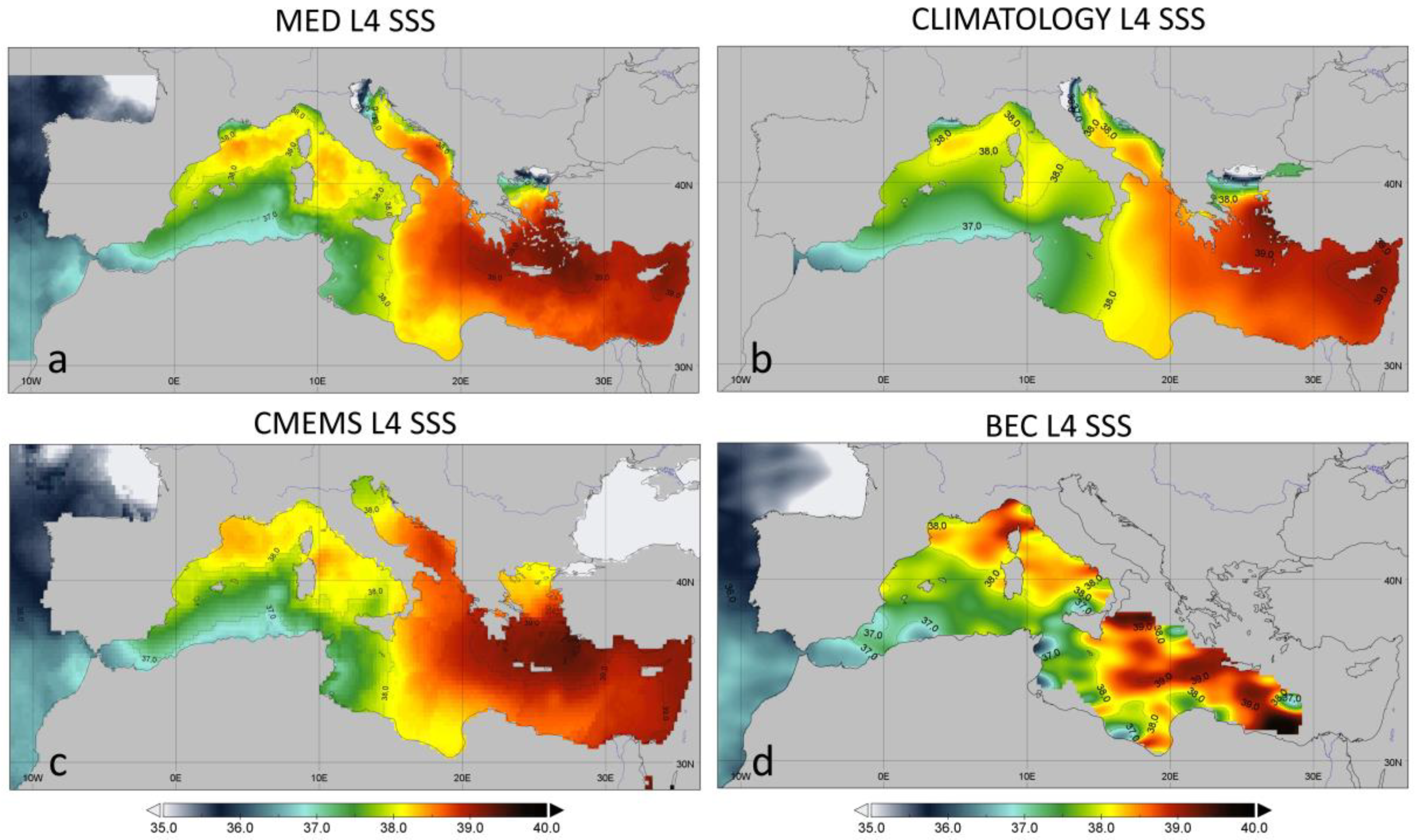
  • A third dataset is based on a weekly global gap-free Level-4 (L4) analyses of the SSS and SSD at 0.25° × 0.25° of resolution, obtained through a multivariate optimal interpolation algorithm that combines SMOS satellite images and in situ salinity measurements with satellite SST information (hereafter, CMEMS L4 SSS, see Figure 2c) [22,24,25]. The product is developed by the CNR and distributed by the CMEMS platform (MULTIOBS_GLO_PHY_S_SURFACE_MYNRT_015_013; see reference to the CMEMS QUID in data availability statement section). Here, these data have been used to build the background SSS field and to obtain pseudo-observations in input to the interpolation (see Section 2.5). The product has been, also, used as a reference for the validation of the Med L4 SSS.
  • An additional SSS dataset has been considered for the comparison with the new Med L4 SSS field. This comprises the daily maps (2010–2016) of interpolated Mediterranean L4 SSS observations at 0.05° × 0.05° resolution (see data availability statement section for more details), produced by the Barcelona Expert Centre (BEC) and the GHER—University of Liege, Belgium [26,31]. This SSS product is retrieved, following a combination of debiased non-Bayesian retrieval, DINEOF, and multifractal fusion, with the SST from the Operational Sea Surface Temperature and Ice Analysis (OSTIA) system, to obtain SMOS SSS fields over the North Atlantic Ocean and the Mediterranean Sea (Figure 2d).

2.4. SST Data

  • The satellite SST dataset used in this work is a daily gap-free (L4) product at high resolution (0.0625°) over the Mediterranean Sea, produced by the GOS-CNR and distributed by CMEMS (SST_MED_SST_L4_NRT_OBSERVATIONS_010_004; see reference to the CMEMS QUID in the data availability statement section). This SST regional product is based on the nighttime images collected by the infrared sensors mounted on different satellite platforms, and covers the southern European Seas [32]. Here, these data have been used in input to the interpolation algorithm.

2.5. Multidimensional Optimal Interpolation

In this work, gap-free regional SSS daily maps are obtained by applying an Optimal Interpolation (OI) method to the synergic combination of in situ and multi-sensor satellite SSS data over the Mediterranean Sea (Figure 2a). OI represents a powerful technique to reconstruct geophysical fields, in case of discontinuous and discrete observations. The principles of OI start from the computation of the desired values ( x analysis ) at the interpolation grid point, as a weighted sum of the anomalies of N observations ( y observed ), with respect to the first guess represented by the background ( x first _ guess ):
x analysis = x first _ guess + C R + C 1 y observed x first _ guess
where C represents the background error covariance, and R represents the observation error covariance (here, assumed diagonal, meaning that observation errors are uncorrelated, with constant values per each observation type/platform):
C = E ε fg ε fg T = E x first _ guess x true x first _ guess x true T
R = E ε obs ε obs T = E y observed x true y observed x true T
The OI method also allows us to compute the variance of the error of the optimal analysis field x analysis :
OI error = 1 C R + C 1
Following the same OI scheme adopted by Droghei et al. [25] and Buongiorno Nardelli et al. [22], the observation error covariance R is expressed here as a noise-to-signal ratio (dividing it by signal variance).
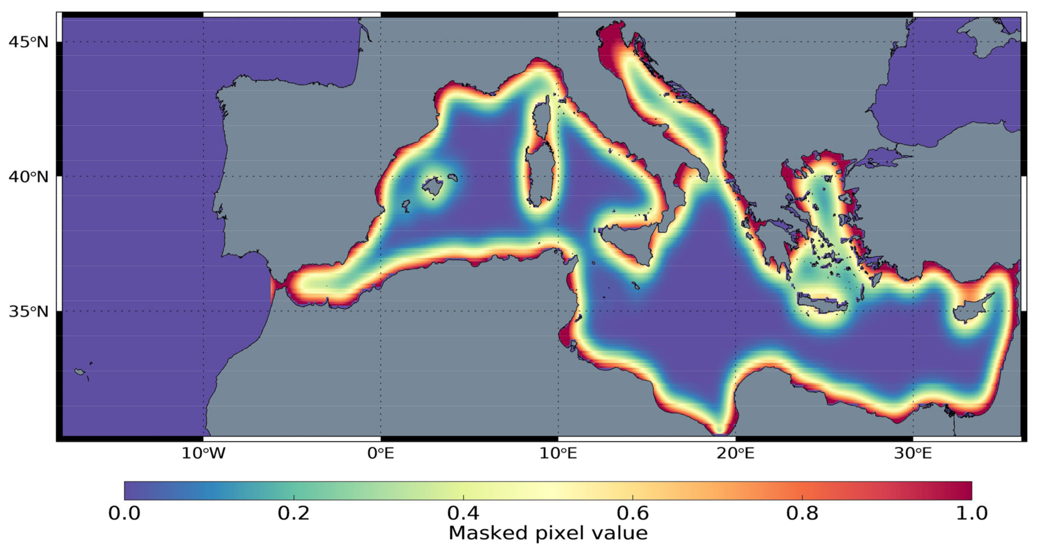
Our background field is obtained by blending an in situ monthly climatology and CMEMS SSS L4 weekly product (see Section 2.2). Specifically, both datasets have been, first, remapped on the output grid resolution (1/16° × 1/16°), through a 2D cubic-spline interpolation, then, the weekly fields were linearly interpolated in time and successively combined with the climatology. More in detail, to reduce the errors and improve the quality of L4 SSS Mediterranean product in the coastal areas, a specific mask was applied to build up the background (Figure 3). Following Equation (5), the weekly background data are gradually replaced by in situ monthly climatology, moving from offshore toward the coastal areas.
background = SSS climatology ×   mask + SSS CMEMS × 1 mask
The background field is, also, used to extract pseudo-observations (with 4-pixel subsampling step) to be included in input to the OI process. As demonstrated by the previous works describing the CMEMS L4 SSS processing chain [22,25], the pseudo-observations allow to “re-modulate” the background field, using the information extracted from the SST pattern, which means that the algorithm can reproduce mesoscale patterns, also, when too sparse observations are available. Here, the in situ observation noise-to-signal ratio was set to 0.05. Conversely, since pseudo-observations are sampled from the background, itself built up by a blend of in situ monthly climatology and CMEMS L4 SSS weekly means, two different fixed values for pseudo-observation errors have been set: a lower value (0.1), for in situ monthly climatology pixels, and a higher error (0.4), for those extracted from CMEMS weekly SSS means.
In principle, the background error covariance should be estimated from all available observations, but in the case of satellite data, this can become too complex, requiring a high computational effort. Therefore, the background error is, usually, approximated by an analytical function of the distance among the samples (here, intended as a Euclidean distance).
However, depending on the system considered and on the available data, covariance models can, also, be extended to multidimensional spaces (e.g., spatio-temporal dimension) directly, including generalised distances (e.g., space/time distances) in the covariance function definition.
In this work, the same model developed by Buongiorno Nardelli et al. [23] has been adopted. This multidimensional covariance model includes, also, high-pass-filtered thermal differences (Δ SST filtered ), in addition to the space-time differences (Δr, Δt), thus forcing the interpolated field to follow the local surface isotherms. In practice, this means that more weight is given to the observations placed on the same isotherm of the interpolation point, with respect to those observations that show the same spatial and temporal differences, but differ for their SST values. Since the SST pattern can provide information about mesoscale dynamics, the inclusion of high-resolution satellite SST represents an effective strategy to improve the resolution of the L4 SSS fields.
C Δ r , Δ t , Δ SST = e Δ r L 2 e Δ t τ 2 e Δ SST filtered T 2
where Δr, Δt, and Δ SST filtered refer to the spatial, temporal, and thermal distances, respectively; L, t, and T represent the spatial, temporal, and thermal decorrelation terms, respectively. In this work, decorrelation and filtering values have been set as the same as those already used in [23], namely L = 500 km, τ = 7 days, and T = 2.75 K.
Additionally, to reduce the computation effort, either in situ or satellite input data are sampled within a searching radius of 1500 km, with a temporal interval of 15 days in the case of in situ measurements, and 3 days in the case of SMOS and SMAP observations, giving priority to the SMAP passages in the filling of the input matrix for the OI process.
The method described above was applied to produce daily Mediterranean L4 SSS fields at 1/16° × 1/16° spatial resolution, over the time window covered by either SMOS or SMAP missions and concurrent in situ independent validation data (2010–2020).

2.6. Metrics Used for Statistical Assessment of the Interpolated SSS Fields

The assessment of the Med L4 SSS product and the comparison of the other L4 SSS fields, with respect to the same in situ independent dataset, is based on the metrics reported in the following Table 1:

3. Results and Discussion

3.1. Validation of the L4 SSS Mediterranean Product and Comparison with the Other L4 SSS Datasets

The new Med L4 SSS product was validated against the independent in situ dataset and compared to the other L4 datasets described in Section 2. Specifically, the accuracy of the new Med L4 SSS fields was compared to that estimated for the Mediterranean climatology, the CMEMS L4 SSS and the BEC L4 SSS products. The total number of matchups, available from 2011 to 2016 for the new algorithm validation and its comparison with the other L4 datasets, is 326,310.
Figure 4a shows the scatterplot of the in situ SSS vs. the new Med L4 SSS fields and the statistical results of this independent validation. Here, the data are mostly distributed along the 1:1 line, with some exceptions for extremely low salinity concentrations. Around the mean Mediterranean salinity values (about 38 pss), the scatterplot indicates a good agreement between observed and interpolated SSS. For lower salinity ranges (<36 pss), instead, the scatter is higher, with interpolated data, generally, overestimating the values provided by the independent in situ observations. In the high SSS ranges (>38 pss), instead, the new Med L4 SSS product shows a reduced scatter, with respect to the climatology and to the other global and regional L4 datasets.
Med L4 SSS and CMEMS L4 SSS products show almost comparable errors. The CMEMS L4 SSS product, produced with the same method applied here for the new Med L4 SSS dataset, differs from the regional product for two main elements: it does not include SMAP data, and it uses a different background. However, the overall evaluation of the Med L4 SSS product shows that the inclusion of coastal in situ climatology in the OI first guess and the ingestion of SMOS/SMAP observations improve the SSS fields for inshore and offshore waters, respectively. This is confirmed by the statistics obtained comparing the regional and global products. The determination coefficient is higher for the Med L4 SSS product (r2 = 0.70) than for the CMEMS L4 product (r2 = 0.62).
Furthermore, while Droghei et al. [25] reported an overall RMSE for CMEMS L4 SSS of 0.84 pss, when estimated from global in situ matchups, the CMEMS L4 SSS RMSE reduces to 0.39 pss, when limiting to the Mediterranean Sea region. The new Med L4 SSS RMSE achieves lower values of around 0.36 pss.
Consistently, the other statistical parameters (i.e., the MeanAPE(%) = 0.56 and MedianAPE(%) = 0.38), also, result slightly better for the new Med L4 SSS product with respect to the CMEMS SSS fields (MeanAPE(%) = 0.58 and MedianAPE(%) = 0.41), except for the bias and MBE(%), which are slightly lower for CMEMS L4 (bias = 0.06 and MBE(%) = 0.13) than those for the new Med L4 SSS dataset (bias = 0.10 pss, MBE(%) = 0.25).
Generally, climatology validation (Figure 4b) displays a larger scatter with respect to that of Med L4 SSS dataset, especially in the high SSS ranges (>38 pss). From a statistical point of view, the errors obtained from the validation of climatology strongly differ from those of the Med L4 SSS dataset. The r2 of 0.64 and RMSE of 0.45 pss, compared to 0.70 and 0.36 pss of the Med L4 SSS, demonstrate a much better performance of our new product. The mean bias of the climatology (0.24 pss) is, also, more than twice the one obtained from the Med L4 SSS validation (0.10 pss).
Nevertheless, at low salinities (<35.5 pss), the distribution of climatological SSS values is consistent with that of the Med L4 SSS samples. This is a direct consequence of the ingestion of the climatology as first guess in the OI process, which allows the Med L4 SSS product to improve in the low salinity ranges, while remaining not well represented in the other two interpolated products, namely CMEMS and BEC L4 SSS. This is evident from Figure 4c,d, where, for in situ SSS values between 30 and 34 pss, CMEMS and BEC L4 products never reproduce salinities below 37.5–38.5 pss.
However, even if climatology can be more accurate in very coastal areas, it cannot precisely resolve the lowest SSS values either, as those are driven by local river discharge variations and related small scale dynamics (i.e., spanning from submesoscale O (~1 km) to small mesoscale O (~10 km) processes). In fact, Figure 4a,b shows that either the in situ climatology or the new Med L4 SSS product cannot correctly retrieve values lower than 35.5–36 pss.
Finally, the independent in situ validation dataset is, also, compared with the BEC Mediterranean L4 SSS fields. As shown in Figure 4d, the scatter of the data is larger than that observed for the new Med L4 SSS in Figure 4a and also for the climatology and CMEMS products (Figure 4b,c). BEC L4 SSS statistics are comparable with those associated with in situ climatology, but significantly differ from that obtained by the new Med and CMEMS L4 SSS products. A noticeable difference is represented by the BEC L4 determination coefficients, attaining around 0.50 vs the 0.70 and 0.62 of the Med L4 SSS and CMEMS datasets, respectively. Similarly, the RMSE of 0.48 pss obtained for BEC L4 SSS dataset is higher than the 0.36 pss and 0.45 pss of the Med L4 product and in situ climatology, respectively. Differing from all the other datasets analysed, the BEC L4 SSS displays a significantly larger spread, even in the highest in situ salinity ranges (>0.38 pss), as visible in Figure 4d.
Besides the statistics emerging from the validation vs independent in situ data, our new Med L4 SSS dataset and the BEC L4 SSS dataset are quite different in their temporal and spatial coverage. The BEC Mediterranean L4 SSS provides data from 2011 to 2016 only, with a spatial domain that does not include the Adriatic Sea and most of the eastern basin. On the contrary, the new Med L4 SSS dataset is available for the full period from 2010 to 2020, covering the entire Mediterranean basin.
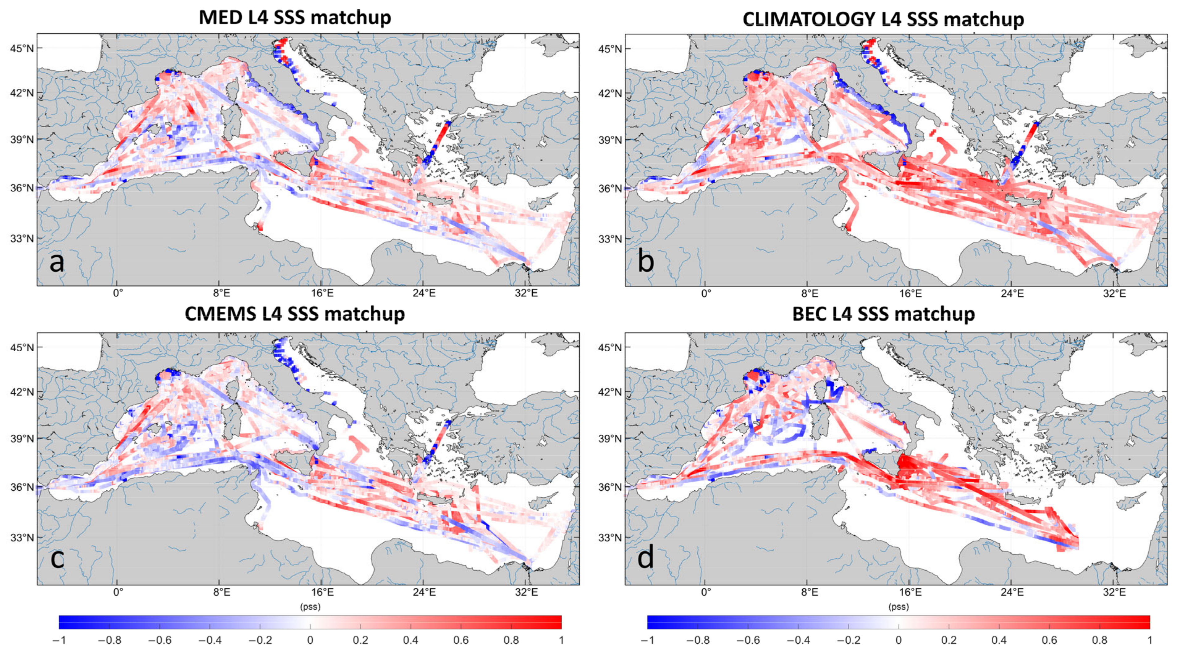
To spatially visualise the differences between in situ and each L4 SSS dataset, in all validation matchups, four different maps have been created and given in Figure 5.
As a direct consequence of how the background has been built up and, then, ingested in the optimal interpolation algorithm, in open waters, the new Med L4 SSS dataset shows similar biases to those of the CMEMS L4 SSS product, while, in more coastal areas, the errors are closer to those observed in the climatology L4 SSS. These similarities between climatology and new Med L4 SSS are, particularly, evident along the Tyrrhenian coasts and in the North Adriatic Sea (Figure 5a,b). In the North Adriatic, either climatology L4 SSS and the new Med L4 SSS underestimates the in situ observations, with the exception of the Po River estuary, where both interpolated fields give estimates higher than the in situ samples, leading to negative biases.
Conversely, in the Adriatic Sea, the CMEMS L4 SSS shows negative differences with respect to the in situ observations, in both coastal and open waters (Figure 5c). In the open waters of the central western Mediterranean basin, the new Med L4 SSS biases are close to zero and lower than those of Climatology and, also, BEC L4 SSS fields, which still underestimate the SSS in situ observations. All four datasets show positive biases in most of the stations of the northwestern Mediterranean Sea, with different magnitudes: higher for Climatology, followed by BEC L4 SSS products, and lower for Med and CMEMS L4 SSS fields (Figure 5).
Among all four datasets, the major differences are observed in the eastern basin. Here, the BEC L4 SSS dataset displays the highest positive biases, followed by Climatology (Figure 5b,d). In the extreme eastern side, both the new Med L4 SSS and CMEMS L4 SSS show very low errors, sometimes close to zero (Figure 5a,c), once again underlying the big potentiality in using these products, also, in those areas of the basin that are characterised by higher biases in satellite SSS measurements, mostly due to radar interferences.
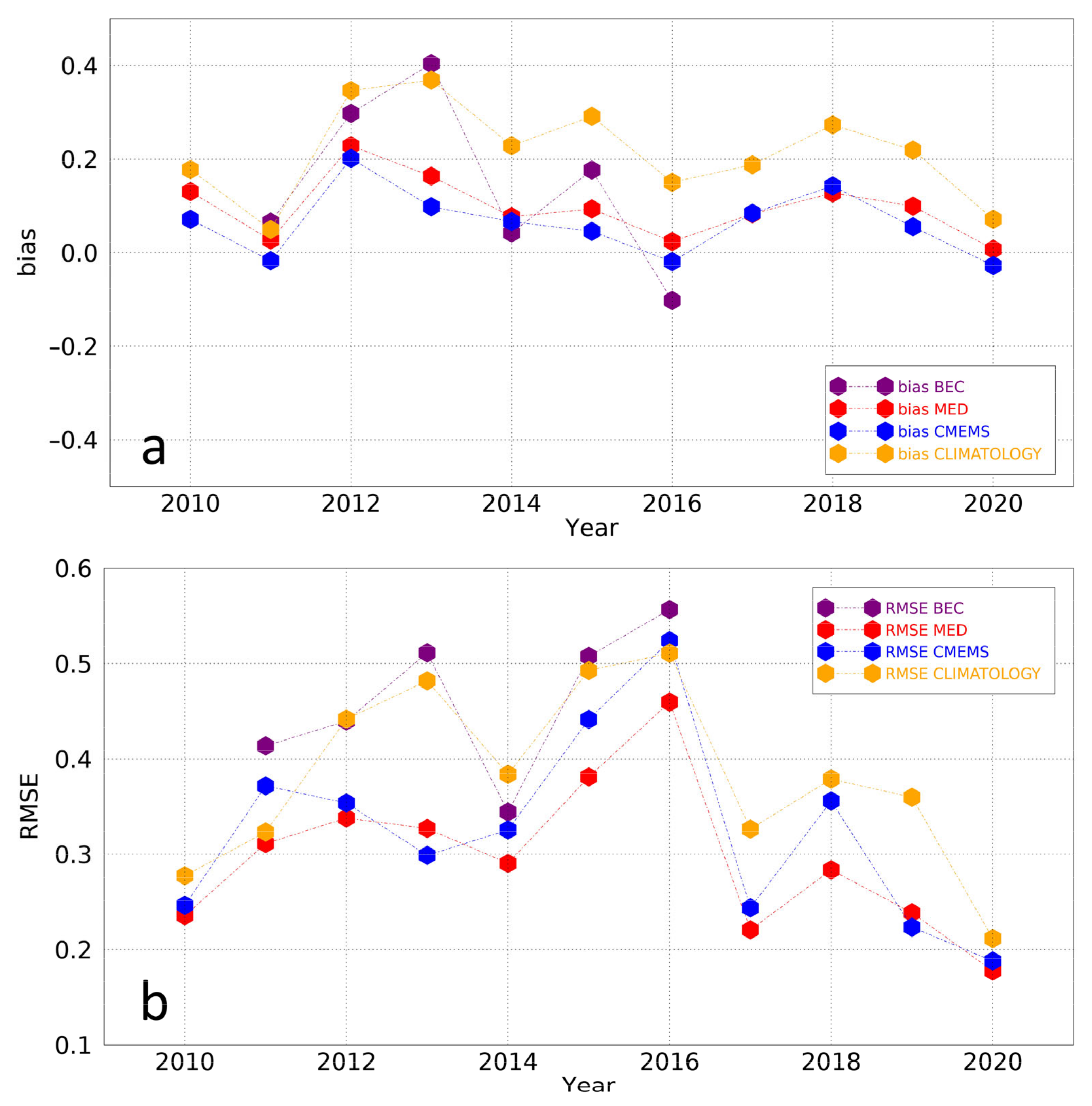
In Figure 6a, the mean biases of the Med L4 SSS are close to those obtained for the CMEMS L4 SSS for all the years. On the contrary, climatology biases are higher than the Med L4 SSS throughout the time series, followed by the BEC L4 SSS dataset, for which only five years can be considered in the comparison.
In Figure 6b, the interannual variability of the RMSE shows higher discrepancies among the four datasets, with respect to those observed in terms of biases. The RMSE of the CMEMS L4 SSS is now less close to the RMSE of the Med L4 SSS, which still remains the dataset with the lowest error throughout the time series. From Figure 6b, it can be, also, highlighted that the inclusion of SMAP observations after 2015 does not appear to impact the statistical results obtained by the Med L4 SSS product throughout the time series. These estimations, however, clearly reflect, also, the different spatial coverage by TSG data over time.

3.2. Power Spectral Density Analysis

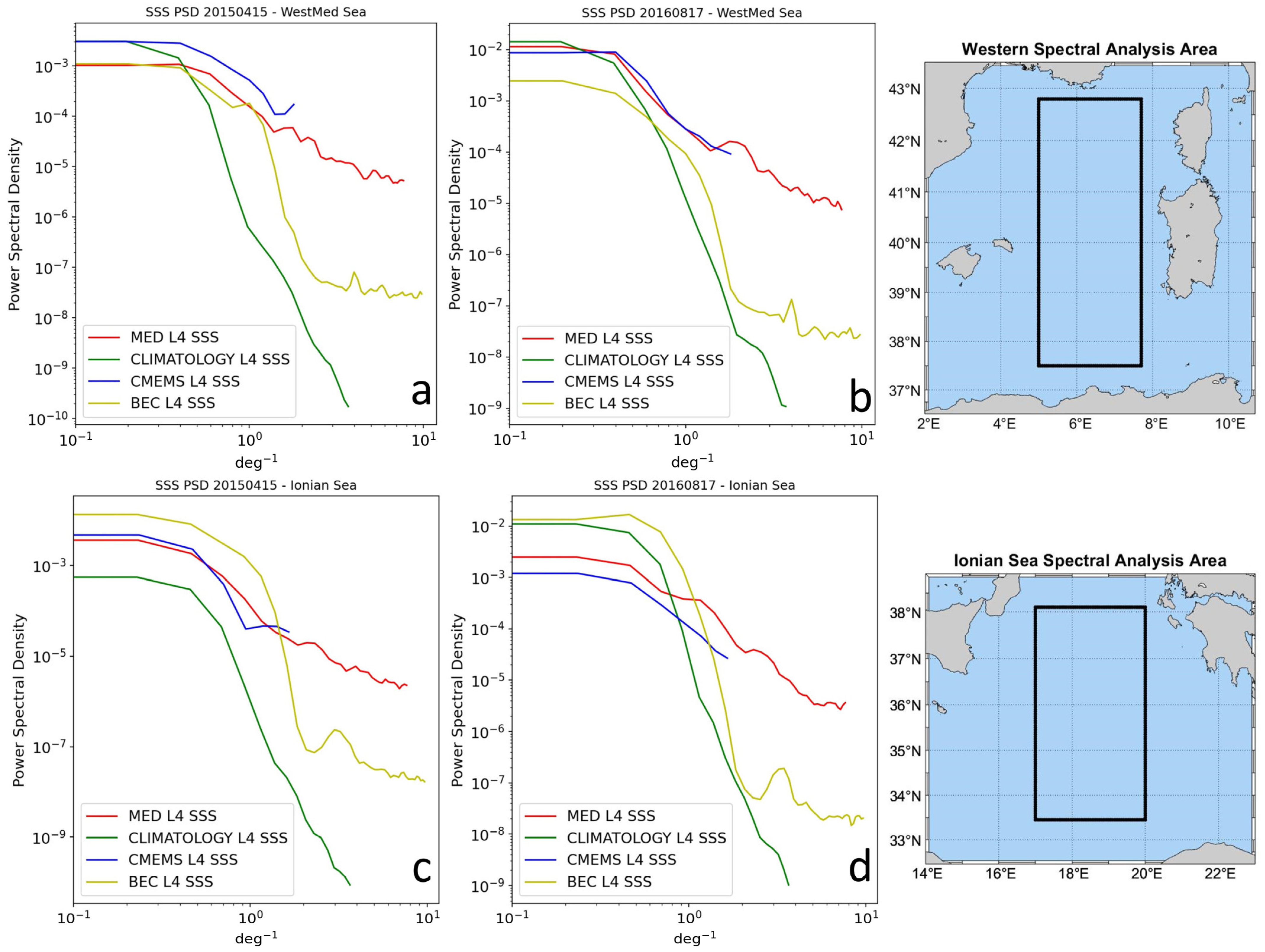
Figure 7 shows the spatial power spectral densities (PSD) as a function of the frequency computed for each of the four L4 SSS datasets.
In order to simplify the comparison between the effective resolution resolved by each product, two example dates (mid-April and August) and two different boxes (one in the western basin and the other in the Ionian Sea) have been considered. The PSD were computed, following the latitudinal variations and averaging the results obtained for each longitude, to provide a single spectrum. Before computing the Fast Fourier Transform, the data were detrended (using a linear fit) and a Blackman-Harris windowing function was applied to diminish the spectral leakage.
As expected, the PSD analysis has highlighted that for both dates and areas, the climatology L4 SSS shows the steepest decrease among all the datasets, with a drop in variance, already, from medium scales, at about 0.5 deg−1 (about 200 km). According to the natural smoothness of such climatological fields, at smaller scales (>2.5–3 deg−1) the climatology L4 SSS collapses, reaching the lowest variance with respect to all other datasets.
The spectrum of the BEC L4 SSS shows an abrupt drop, at approximately 1–1.5 deg−1, with a variance that still decreases until smaller scales (>3 deg−1), where the signal finally flattens and reveals a noise at small scales.
Compared with the BEC L4 SSS, which has the highest nominal grid resolution, CMEMS L4 SSS and Med L4 SSS display the highest spatial variance in the mesoscale wavelength ranges (>1.5–2 deg−1) for both the western and Ionian Sea areas (Figure 7).
Even with different magnitudes, all the spectra show the same shape in the two different areas and dates, with a pronounced slope for climatology and BEC L4 SSS as well as a gentler decrease for CMEMS and Med L4 SSS products.
The Med L4 SSS field, though, clearly achieves the highest effective spatial resolution, with the spectrum flattening less steeply than that of BEC L4 SSS.
In terms of resolved scales, the results of the PSD analysis provided evidence of the improvements that can be reached, by applying the multidimensional OI to a combination of in situ/satellite data.
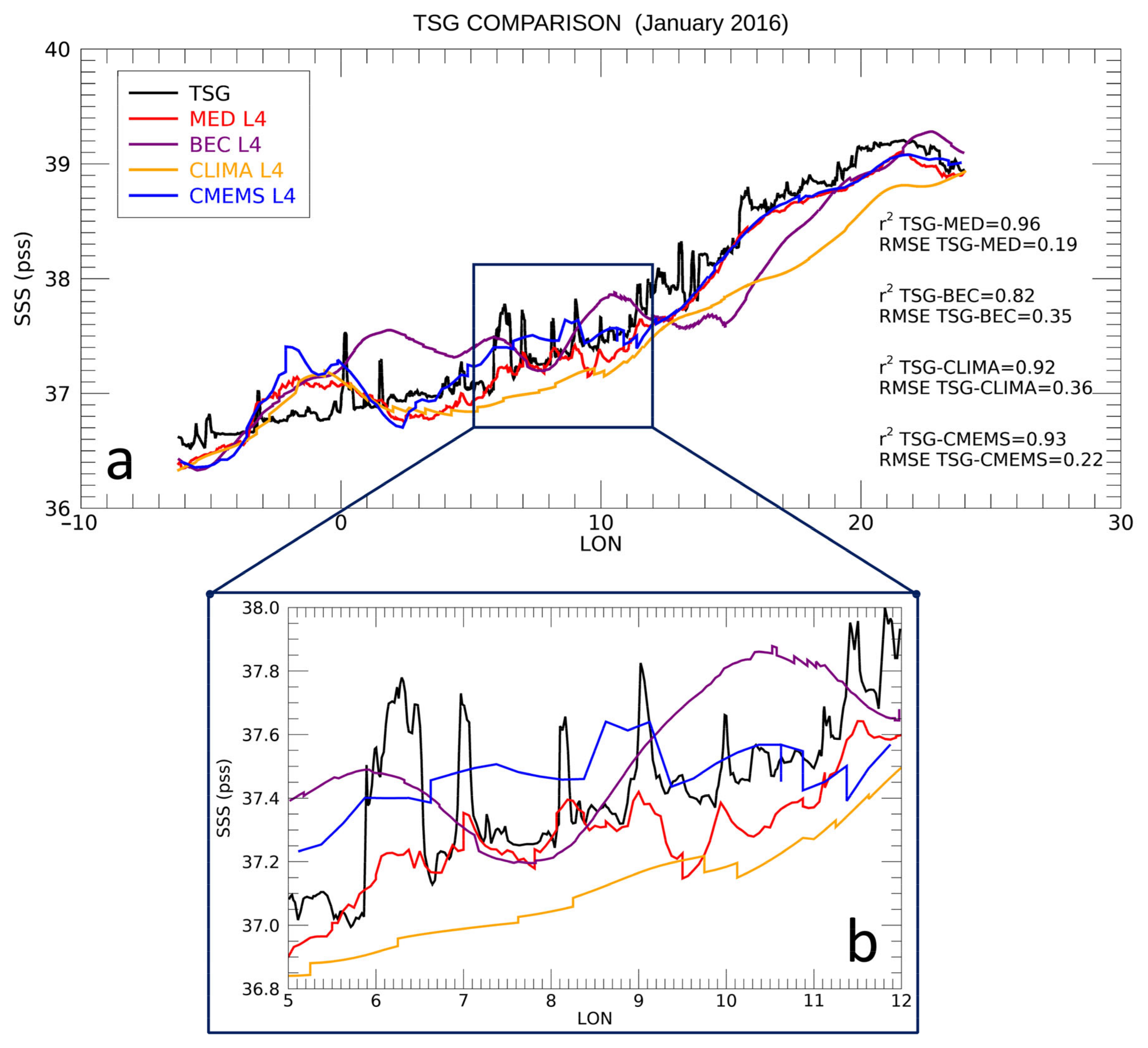
To further support the PSD results and to demonstrate that the signal obtained for the Med L4 SSS dataset does not originate from noise or artefacts, two examples of observed transect are displayed in Figure 8 and Figure 9. The transects were selected along a trans-Med trajectory, and in two distinct seasons (January and August), in order to represent the highest SSS spatial and temporal variability. The SSS field of January is, usually, the result of more variable upper-ocean dynamics (related to smaller sub-mesoscale emergence, caused by the reduced Rossby radius of deformation), while August can reveal a different surface signal because of the more marked stratification of the water column.
In Figure 8a, the TSG trajectory is compared with the SSS values extracted from the four datasets. As expected, climatology shows the smoothest signal, with the lowest statistical performance as revealed by the determination coefficient and RMSE reported in Figure 8a. Even though displaying a higher variability, the BEC L4 SSS product shows a wider discrepancy, with respect to the CMEMS L4 and Med L4 SSS fields. This is, particularly, evident between 0° and 5°E. In the first section of the transect (−6°E to 5°E), all four datasets are far from the TSG signal, while in the last section, only the new Med L4 SSS and CMEMS L4 SSS products get close to the in situ measurements. The most interesting section is within 5–11°E, where the TSG signal is more variable. A zoom of this area (Figure 8b) allows to visualise the small-scale variability of the TSG signal. Among all datasets, the new Med L4 SSS, clearly, outperforms the others in reproducing several structures at a few km scales. Indeed, even with some differences in magnitude, the Med L4 SSS field reproduces most of the picks visible in the TSG track. The good performance of the Med L4 SSS dataset, in reproducing the TSG observed values, is also supported by the statistics computed along the transect (Figure 8a).
As shown in Figure 8b, there is a significant improvement in the Med L4 SSS dataset with respect to the standard global and regional products.
Similar results are obtained for the same trajectory sampled in a different season (Figure 9). In that case, the amplitude of the signal is more variable, however, both Med L4 SSS and CMEMS L4 SSS are closer to the observed TSG values than the BEC L4 SSS and climatology. Consistently, with its relative spatial resolution, the CMEMS L4 SSS shows a smoothest signal than the Med L4 SSS, which, still, presents the best statistics among all datasets.

3.3. Sea Surface Salinity Trend over 2010–2020 Decade

The availability of a long time series of the new Med L4 SSS product allowed an analysis of the spatial and temporal variability of the salinity fields in the Mediterranean region. The trend analysis was carried out, by using an X-11 seasonal adjustment process, following the same approach adopted in [33,34].
The seasonal adjustment process requires as input a time series X t (namely an SSS monthly time series), which is then decomposed as follow:
X t = T t + S t + I t
where T t is the trend component, S t the seasonal component, and I t the irregular component, which accounts for the residual irregular variations, such as sub-annual fluctuations. The deseasonalisation of the time series is obtained by applying, iteratively, running averages, which act as a low-pass filter for T t and S t estimation from X t .
The X-11 method is a three-step filtering algorithm. The first step foresees the application of a centered 13-term moving average (MA) on X t , as given in Equation (8):
T t 1 = MA 2 × 12 X t
Then, a first estimate of the seasonal component is obtained by applying a centered five-term seasonal moving average filter (SMA3×3) to the detrended time series, Z t = X t T t 1 , as described in Equation (9):
S t 0 = MA 3 × 3 Z t
From Equation (9), the resulting seasonal component S t 1 is adjusted by subtracting its annual-centered running mean, S t 1 = S t 0 S t 0 , producing an approximately zero-mean seasonality.
The second step foresees the application of the repeated passages of the first steps on the seasonally adjusted series, Y t = X t S 1 t , as follows; T t 2 = MA 2 × 12 Y t   and   S t 2 = MA 3 × 5 Z t 1 , where MA3×5 is a centered seven-term seasonal moving average filter, and Z t 1 = X t T t 2 the detrended time series. The seasonal signal S t 2   is, then, adjusted again, to have zero mean.
The third step provides the final trend component, T t 3 = MA 2 × 12 Y t , with Y t = X t S t 2 , and the residual component as I t = X t S t 2 T t 3 .
The main advantage of the X-11 approach relies on computing the annual cycle on a year-to-year basis and not as a fixed mean effect, as in the traditional trend computation algorithms.
Once computed the seasonal adjustment, the magnitude and significance of the trend is estimated, by applying the Mann–Kendall (MK) test and Sen’s method [35] to T t . The MK test is rank-based and non-parametrical, used to identify either upward or downward trends, while Sen’s method is used to estimate the slope of the trend, as the median of the slopes of all pairwise differences in the T t series (see Appendix A) [34].
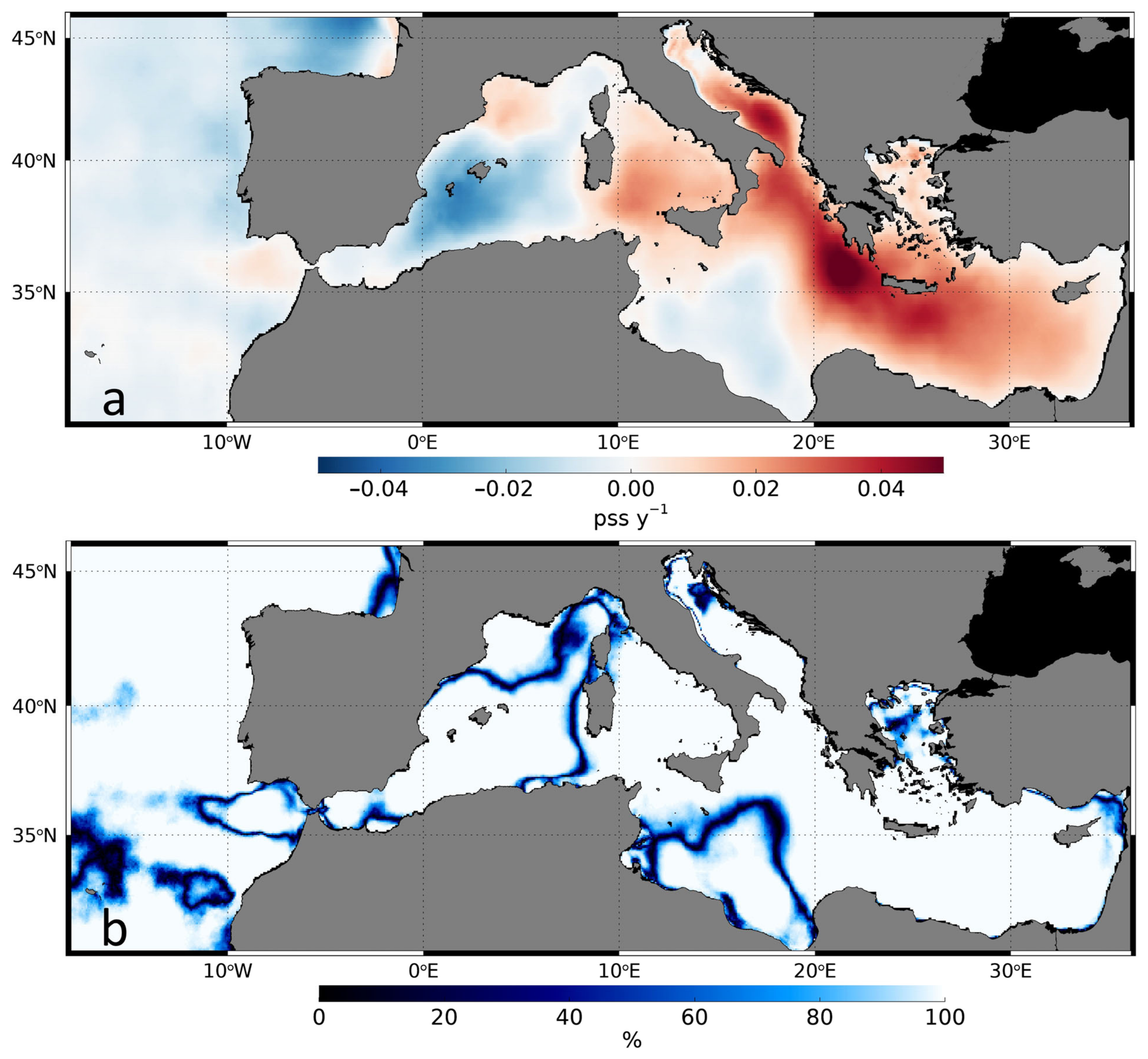
The spatial variation of the SSS trend and its significance level is shown in Figure 10. It highlights a different pattern between western and eastern basins. Overall, a marked salinity increase is found in the eastern basin. Negative values are present along the North African coast, reducing from the western basin to the Ionian Sea. This is, particularly, evident south of the Balearic Islands, where the trend attains values around −0.03 pss y−1, with a high significance level (about 99%).
A weak positive trend is seen in the Gulf of Lion, while more intense positive values cover the whole Tyrrhenian Sea. The positive trend reaches its maxima (about 0.05 pss y−1) in the southern Adriatic Sea and in the Levantine Sea. Here, the trend shows a high significance level with a uniform pattern.
Though considering time series of different lengths, the trend analysis over the 2010–2020 decade reveals a Levantine salinification that is consistent with what was observed by Grodsky et al. [36], in the years 2015–2019. Clearly, the trend pattern in Figure 10 cannot be directly compared to that described by Grodsky et al. [36] because of the temporal extension of the series. Moreover, our trend estimates (0.05 pss y−1) are lower than the values of SMAP SSS linear tendency observed in Grosky et al. [36] (about 0.14 pss y−1). In the OI algorithm, the adjustment of the satellite SSS fields with in situ observations can explain a discrepancy in the trend magnitude. Nevertheless, even with different magnitudes, our trend pattern is consistent with Grodsky et al. [36].
Indeed, estimating the trends on the same 2015–2019 time window (not shown), positive values are found along the Libya coast, and negative values are found in the northwestern Ionian Sea, confirming what was, already, pointed out by Grodsky et al. [36], who suggest that the pattern of salinification in the Levantine observed during that period may be a consequence of the strengthening of anticyclonic circulation in the Ionian Sea (an increase of the BiOS amplitude) and the strengthening of winds due to an enhanced NAO atmospheric pressure pattern.

4. Conclusions

The monitoring of SSS, in a relatively small but dynamically relevant basin as the Mediterranean Sea, is crucial for a more comprehensive understanding of climate change at regional scales and for the assessment of its impact on the global scales. Given the sparseness of in situ SSS data, only the synergic combination of in situ and satellite observations can improve the spatial and temporal scales of SSS fields, resolving the smaller scales (mesoscale). In this work, the multivariate OI algorithm, originally proposed by Buongiorno Nardelli et al. [22,23] and Droghei et al. [24,25], has been modified to provide regional daily L4 SSS fields at 1/16° nominal spatial resolution, covering the Mediterranean Sea. The implemented approach combines in situ and multi-sensor satellite observations, exploiting the high resolution of SST satellite data to provide gap-free SSS maps and overcoming the sparseness of in situ datasets.
The main novelties introduced in this updated algorithm are related to the way the first guess is designed, and to the inclusion of SMAP as additional input source of satellite SSS data.
The new Med L4 SSS has been validated against a set of independent in situ SSS observations, which have been used, also, as a further comparison with respect to the other three datasets, namely the in situ monthly climatology, the weekly CMEMS product, and the daily BEC L4 SSS product. It showed an overall RMSE (0.36 pss), which is lower than that obtained for global products (0.39 pss) and climatology (0.45). Compared with the BEC L4 SSS, the Med L4 SSS showed improved statistics and a larger spatial coverage, providing optimally interpolated SSS fields also in the Adriatic Sea and eastern basin. If compared with climatology and BEC L4 SSS, a reduction in biases between Med L4 SSS and in situ observations is, particularly, evident in open waters; while in the north Adriatic Sea, the new Med L4 SSS algorithm proved capable of reaching extremely low SSS values. Very low biases are, also, found in the eastern basin, where the detection of satellite SSS is, usually, hindered by land contamination of radio-frequency interference.
The combination of the Mediterranean in situ SSS climatology with the upsized and temporally interpolated CMEMS L4 weekly product, generally reduces the biases, also, in some coastal waters, with respect to those found in the BEC L4 SSS product.
Moreover, the inclusion of SMAP SSS observations significantly improved the coverage of remotely sensed SSS fields, allowing for the first time to cover the entire Mediterranean Sea.
Given the low negative CMEMS L4 SSS biases observed along the Tyrrhenian coasts, one of the possible future improvements of the proposed algorithm will be the creation of a refined mask for the background, allowing to start from in situ monthly climatology only in specific coastal areas (e.g., specific river mouths and the north Adriatic area).
As suggested by the spatial power spectral density analysis, and further demonstrated by an along-trajectory comparison with independent TSG data, the combination of this multivariate approach and multi-sensor satellite data blending with in situ observations leads to a significant improvement of the effective resolution of the final SSS fields. Among all datasets, the new Med L4 SSS showed the highest energy variance at smaller scales (almost mesoscale resolving), also, with respect to the BEC L4 SSS dataset, which is characterised by a higher nominal spatial resolution.
The improved performance of the Med L4 SSS dataset allowed an analysis of the variability in time and space of the salinity fields in the basin. The SSS trend map has been computed by applying the MK and Sen’s methods [35,37,38], on the seasonal adjusted time series. This analysis evidenced a clear salinification of the Levantine Sea in the 2010–2020 decade, accompanied by a slight freshening of the surface waters along the North African coasts, generally associated with the Atlantic water inflow, thus showing a clear west–east gradient. Even with different magnitudes (higher values, about 0.14 pss y−1 for SMAP SSS linear tendency in Grodsky et al. [36], than our trend values, 0.05 pss y−1), the patterns of this salinification are consistent with the results of Grodsky et al. [36].
This work confirms that the multivariate OI combining multi-sensor satellite and in situ observations, along with the high resolution of the SST, is a valuable tool to improve the spatial and temporal resolution of SSS and, consequently, the monitoring of ocean salinity variations at finer scale. This gives a potential opportunity to better understand the dynamical processes that occur at different scales in a complex and peculiar basin, such as the Mediterranean Sea.

Author Contributions

Conceptualization, M.S. and B.B.N.; methodology, B.B.N.; software, M.S. and B.B.N.; validation, M.S.; formal analysis, M.S.; investigation, M.S. and B.B.N.; resources, B.B.N., S.A. and R.S.; data curation, M.S.; writing—original draft preparation, M.S. and B.B.N.; writing—review and editing, M.S., B.B.N. and S.A.; visualization, M.S.; supervision, B.B.N.; project administration, B.B.N. and R.S.; funding acquisition, B.B.N. and R.S. All authors have read and agreed to the published version of the manuscript.

Funding

This research was partially supported by the Copernicus Marine Environment Monitoring Service (CMEMS) Multi-Observation Thematic Assembly Centre (83-CMEMS-TAC-MULTI-OBS).

Data Availability Statement

Most of the data presented in this study are openly available at: https://marine.copernicus.eu/, for the MULTIOBS_GLO_PHY_S_SURFACE_MYNRT_015_013 dataset (QUID also available at https://catalogue.marine.copernicus.eu/documents/QUID/CMEMS-MOB-QUID-015-013.pdf); https://doi.org/10.5281/zenodo.1146974, for the Mediterranean Sea in situ monthly climatology; https://doi.org/10.17882/39475, for the Global Ocean Surface Underway Data (GOSUD) thermo-salinometer (TSG) observation dataset; http://dx.doi.org/10.12770/12dba510-cd71-4d4f-9fc1-9cc027d128b0, for the CATDS-PDC L3OS 2Q-Debiased daily valid ocean salinity values product from the SMOS satellite; https://coastwatch.noaa.gov/cw/satellite-data-products/sea-surface-salinity/smap.html, for the daily L3 SSS SMAP data; http://bec.icm.csic.es/six-years-of-the-new-smos-sss-maps-in-the-mediterranean-sea-now-available/, for the BEC L4 SSS data; and https://doi.org/10.48670/moi-00172, for the SST_MED_SST_L4_NRT_OBSERVATIONS_010_004 dataset (QUID also available at https://catalogue.marine.copernicus.eu/documents/QUID/CMEMS-SST-QUID-010-004-006-012-013.pdf). For all datasets, last accessed on 20 December 2021.

Acknowledgments

We acknowledge the CMEMS project for the distribution of the free in situ and remote sensing data used in this work. We would like to thank the Centre Aval de Traitement des Données SMOS—Production and Dissemination Center, for the distribution of SMOS L3OS 2Q SSS data, and NOAA CoastWatch/OceanWatch for freely providing the SMAP Level-3 gridded sea-surface salinity (SSS) daily mean dataset. We, also, thank all the people involved in the creation and distribution of the Mediterranean atlas and monthly climatology provided by Iona et al. (2018). We, moreover, acknowledge all data providers involved in the GOSUD program, for making their products freely available. We would like to thank Angelo Bonanno and all the people involved in the collection and distribution of the in situ validation data used in this work. A special thanks to Daniele Ciani for his technical support, scientific support, and helpful advice.

Conflicts of Interest

The authors declare no conflict of interest. The funders had no role in the design of the study; in the collection, analyses, or interpretation of data; in the writing of the manuscript; or in the decision to publish the results.

Appendix A

Considering a time series of n observations ( x 1 , x 2 ,   x n ) , the MK is based on the statistical test S and its variance, Var S , as follows:
S = i = 1 n 1   j   = i + 1 n sgn x j ¯ x i
sgn x J x i = 1   if   x j x i > 0 0   if   x j x i = 0 1   if   x j x i < 0
Var S = 1 18 n n 1 2 n + 5 p = 1 q t p t p 1 2 t p + 5
where x i , j are the values of the time series (with j = i + 1 ), n   the number of data, q the number of tied groups (a tied group is a set of samples that have the same value), and t p the number of data points in the p-group.
The statistical significance of the test is given by computing the following Z value:
Z = S 1 Var s   if   S > 0 0                         if   S = 0 S + 1 Var s   if   S < 0
If Z > z 1 α / 2 (with α identifying the chosen significance level), the trend results as significant.
The magnitude of slope β is computed, by using the following Sen’s equation:
β = Median Q k = x j   x i j 1 ,   j > i ;   k = 1 , n n 1 2
with Qk identified as the ensemble of all possible pairs of differences xj − xi in the sample.

References

  1. Reul, N.; Grodsky, S.A.; Arias, M.; Boutin, J.; Catany, R.; Chapron, B. Sea surface salinity estimates from spaceborne L-band radiometers: An overview of the first decade of observation (2010–2019). Remote Sens. Environ. 2020, 242, 111769. [Google Scholar] [CrossRef]
  2. Bergamasco, A.; Malanotte-Rizzoli, P. The circulation of the Mediterranean Sea: A historical review of experimental investigations. Adv. Oceanogr. Limnol. 2010, 1, 11–28. [Google Scholar] [CrossRef]
  3. Skliris, N.; Zika, J.D.; Herold, L.; Josey, S.A.; Marsh, R. Mediterranean sea water budget long-term trend inferred from salinity observations. Clim. Dyn. 2018, 51, 2857–2876. [Google Scholar] [CrossRef] [Green Version]
  4. Lozier, M.S.; Sindlinger, L. On the Source of Mediterranean Overflow Water Property Changes. J. Phys. Oceanogr. 2009, 39, 1800–1817. [Google Scholar] [CrossRef] [Green Version]
  5. Potter, R.A. On the warming and salinification of the Mediterranean outflow waters in the North Atlantic. Geophys. Res. Lett. 2004, 31, L01202. [Google Scholar] [CrossRef] [Green Version]
  6. Skliris, N. Past, present and future patterns of the Thermohaline Circulation and characteristic water masses of the Mediterranean Sea. In The Mediterranean Sea; Goffredo, S., Dubinsky, Z., Eds.; Springer: Berlin/Heidelberg, Germany, 2014; pp. 29–48. [Google Scholar]
  7. Millot, C. Interannual salinification of the Mediterranean inflow. Geophys. Res. Lett. 2007, 34, L21609. [Google Scholar] [CrossRef]
  8. Vinogradova, N.; Lee, T.; Boutin, J.; Drushka, K.; Fournier, S.; Sabia, R. Satellite Salinity Observing System: Recent Discoveries and the Way Forward. Front. Mar. Sci. 2019, 6, 243. [Google Scholar] [CrossRef]
  9. Kontakiotis, G.; Besiou, E.; Antonarakou, A.; Zarkogiannis, S.D.; Kostis, A.; Mortyn, P.G. Decoding sea surface and paleoclimate conditions in the eastern Mediterranean over the Tortonian-Messinian Transition. Palaeogeogr. Palaeoclimatol. Palaeoecol. 2019, 534, 109312. [Google Scholar] [CrossRef]
  10. Kontakiotis, G.; Butiseacă, G.A.; Antonarakou, A.; Agiadi, K.; Zarkogiannis, S.D.; Krsnik, E. Hypersalinity accompanies tectonic restriction in the eastern Mediterranean prior to the Messinian Salinity Crisis. Palaeogeogr. Palaeoclimatol. Palaeoecol. 2022, 592, 110903. [Google Scholar] [CrossRef]
  11. Vasiliev, I.; Karakitsios, V.; Bouloubassi, I.; Agiadi, K.; Kontakiotis, G.; Antonarakou, A. Large Sea Surface Temperature, Salinity, and Productivity-Preservation Changes Preceding the Onset of the Messinian Salinity Crisis in the Eastern Mediterranean Sea. Paleoceanogr. Paleoclimatol. 2019, 34, 182–202. [Google Scholar] [CrossRef]
  12. Maes, C.; Behringer, D.; Reynolds, R.W.; Ji, M. Retrospective Analysis of the Salinity Variability in the Western Tropical Pacific Ocean Using an Indirect Minimization Approach. J. Atmos. Ocean Technol. 2000, 17, 13. [Google Scholar] [CrossRef]
  13. Buongiorno Nardelli, B.; Santoleri, R. Reconstructing Synthetic Profiles from Surface Data. J. Atmos. Ocean Technol. 2004, 21, 11. [Google Scholar]
  14. Guinehut, S.; Le Traon, P.Y.; Larnicol, G.; Philipps, S. Combining Argo and remote-sensing data to estimate the ocean three-dimensional temperature fields—A first approach based on simulated observations. J. Mar. Syst. 2004, 46, 85–98. [Google Scholar] [CrossRef]
  15. Buongiorno Nardelli, B.; Santoleri, R. Methods for the Reconstruction of Vertical Profiles from Surface Data: Multivariate Analyses, Residual GEM, and Variable Temporal Signals in the North Pacific Ocean. J. Atmos. Ocean Technol. 2005, 22, 1762–1781. [Google Scholar] [CrossRef]
  16. Buongiorno Nardelli, B.; Cavalieri, O.; Rio, M.-H.; Santoleri, R. Subsurface geostrophic velocities inference from altimeter data: Application to the Sicily Channel (Mediterranean Sea). J. Geophys. Res. 2006, 111, C04007. [Google Scholar] [CrossRef]
  17. Ballabrera-Poy, J.; Mourre, B.; Garcia-Ladona, E.; Turiel, A.; Font, J. Linear and non-linear T–S models for the eastern North Atlantic from Argo data: Role of surface salinity observations. Deep Sea Res. Part Oceanogr. Res. Pap. 2009, 56, 1605–1614. [Google Scholar] [CrossRef]
  18. Bao, S.; Zhang, R.; Wang, H.; Yan, H.; Yu, Y.; Chen, J. Salinity Profile Estimation in the Pacific Ocean from Satellite Surface Salinity Observations. J. Atmos. Ocean Technol. 2019, 36, 53–68. [Google Scholar] [CrossRef]
  19. Su, H.; Yang, X.; Lu, W.; Yan, X.-H. Estimating Subsurface Thermohaline Structure of the Global Ocean Using Surface Remote Sensing Observations. Remote Sens. 2019, 11, 1598. [Google Scholar] [CrossRef] [Green Version]
  20. Buongiorno Nardelli, B. A Deep Learning Network to Retrieve Ocean Hydrographic Profiles from Combined Satellite and In Situ Measurements. Remote Sens. 2020, 12, 3151. [Google Scholar] [CrossRef]
  21. Umbert, M.; Hoareau, N.; Turiel, A.; Ballabrera-Poy, J. New blending algorithm to synergize ocean variables: The case of SMOS sea surface salinity maps. Remote Sens. Environ. 2014, 146, 172–187. [Google Scholar] [CrossRef]
  22. Buongiorno Nardelli, B.; Droghei, R.; Santoleri, R. Multi-dimensional interpolation of SMOS sea surface salinity with surface temperature and in situ salinity data. Remote Sens. Environ. 2016, 180, 392–402. [Google Scholar] [CrossRef]
  23. Buongiorno Nardelli, B. A Novel Approach for the High-Resolution Interpolation of In Situ Sea Surface Salinity. J. Atmos. Ocean Technol. 2012, 29, 867–879. [Google Scholar] [CrossRef]
  24. Droghei, R.; Nardelli, B.B.; Santoleri, R. Combining in Situ and Satellite Observations to Retrieve Salinity and Density at the Ocean Surface. J. Atmos. Ocean Technol. 2016, 33, 1211–1223. [Google Scholar] [CrossRef]
  25. Droghei, R.; Buongiorno Nardelli, B.; Santoleri, R. A New Global Sea Surface Salinity and Density Dataset from Multivariate Observations (1993–2016). Front. Mar. Sci. 2018, 5, 84. [Google Scholar] [CrossRef] [Green Version]
  26. Olmedo, E.; Taupier-Letage, I.; Turiel, A.; Alvera-Azcárate, A. Improving SMOS Sea Surface Salinity in the Western Mediterranean Sea through Multivariate and Multifractal Analysis. Remote Sens. 2018, 10, 485. [Google Scholar] [CrossRef] [Green Version]
  27. Kolodziejczyk, N.; Diverres, D.; Jacquin, S.; Gouriou, Y.; Grelet, J.; Le Menn, M.; Tassel, J.; Reverdin, G.; Maes, C.; Gaillard, F. Sea Surface Salinity from French RESearcH Vessels: Delayed mode dataset, annual release. SEANOE 2021. [Google Scholar] [CrossRef]
  28. Iona, A.; Theodorou, A.; Watelet, S.; Troupin, C.; Beckers, J.-M.; Simoncelli, S. Mediterranean Sea Hydrographic Atlas: Towards optimal data analysis by including time-dependent statistical parameters. Earth Syst. Sci. 2018, 10, 1281–1300. [Google Scholar] [CrossRef] [Green Version]
  29. Fore, A.; Yueh, S.; Tang, W.; Hayashi, A. SMAP Salinity and Wind Speed Data User’s Guide; California Institute of Technology: Pasadena, CA, USA, 2020; p. 42. [Google Scholar]
  30. NASA Jet Propulsion Laboratory (NASA/JPL). JPL SMAP Level 2B near Real-time CAP Sea Surface Salinity V5.0 Validated Dataset 2020. Available online: https://podaac.jpl.nasa.gov/dataset/SMAP_JPL_L2B_NRT_SSS_CAP_V5 (accessed on 3 April 2022).
  31. BEC Team. SMOS-BEC Mediterranean Region SSS Product Description; Instituto de Ciencias del Mar (ICM)—CSIC: Barcelona, Spain, 2019. [Google Scholar]
  32. Buongiorno Nardelli, B.; Tronconi, C.; Pisano, A.; Santoleri, R. High and Ultra-High resolution processing of satellite Sea Surface Temperature data over Southern European Seas in the framework of MyOcean project. Remote Sens. Environ. 2013, 129, 1–16. [Google Scholar] [CrossRef]
  33. Colella, S.; Falcini, F.; Rinaldi, E.; Sammartino, M.; Santoleri, R. Mediterranean Ocean Colour Chlorophyll Trends. PLoS ONE 2016, 11, e0155756. [Google Scholar] [CrossRef] [Green Version]
  34. Pisano, A.; Marullo, S.; Artale, V.; Falcini, F.; Yang, C.; Leonelli, F.E. New Evidence of Mediterranean Climate Change and Variability from Sea Surface Temperature Observations. Remote Sens. 2020, 12, 132. [Google Scholar] [CrossRef] [Green Version]
  35. Sen, P.K. Estimates of the Regression Coefficient Based on Kendall’s Tau. J. Am. Stat. Assoc. 1968, 63, 1379–1389. [Google Scholar] [CrossRef]
  36. Grodsky, S.A.; Reul, N.; Bentamy, A.; Vandemark, D.; Guimbard, S. Eastern Mediterranean salinification observed in satellite salinity from SMAP mission. J. Mar. Syst. 2019, 198, 103190. [Google Scholar] [CrossRef]
  37. Kendall, M. Multivariate Analysis; Charles Griffin b Co. Ltd.: London, UK; High Wycombe, UK, 1975; Volume 19, p. 309. [Google Scholar] [CrossRef]
  38. Mann, H.B. Nonparametric Tests against Trend. Econometrica 1945, 13, 245–259. [Google Scholar] [CrossRef]
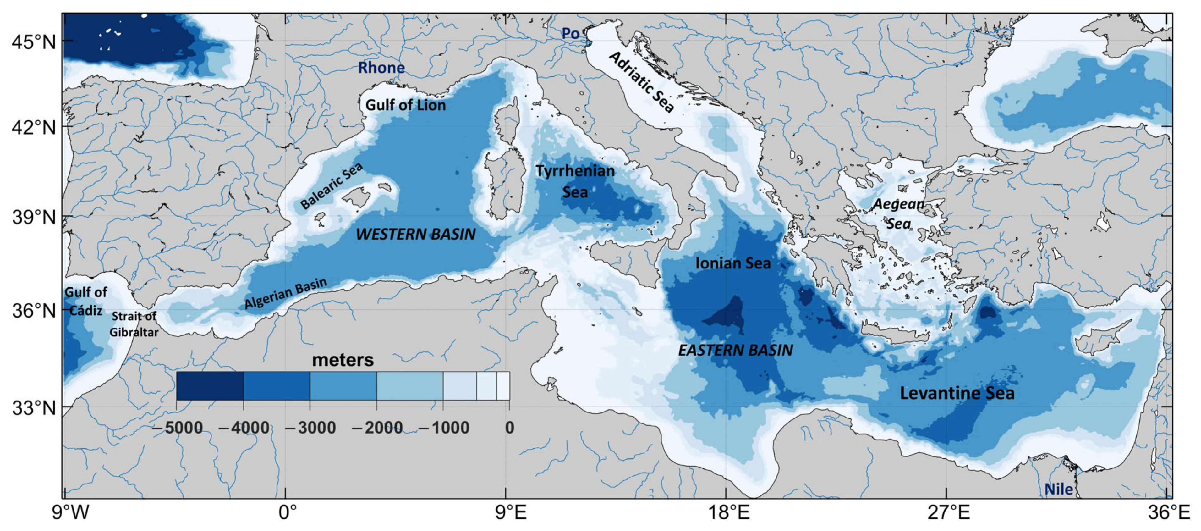
Figure 1. Map of the Mediterranean Sea bathymetry, showing the main basins, sea regions, and major rivers.
Remotesensing 14 02502 g001
Figure 2. (a) Example of daily new Med L4 SSS field (20 April 2016); (b) in situ monthly climatology (April); (c) weekly CMEMS L4 SSS product (centered on 20 April 2016); and (d) corresponding daily BEC L4 SSS product (20 April 2016).
Remotesensing 14 02502 g002
Figure 3. Map of the mask used to build the background from the blending of in situ monthly climatology and weekly CMEMS L4 SSS.
Remotesensing 14 02502 g003
Figure 4. Scatterplots of the validation against the independent in situ dataset. Comparison of the observed against interpolated L4 SSS values, for the four different L4 SSS datasets: new Med L4 SSS (a); in situ climatology (b); CMEMS L4 SSS (c); BEC L4 SSS (d). In each panel, the statistics of the validation for each satellite dataset are shown.
Remotesensing 14 02502 g004
Figure 5. Spatial distribution of the validation matchups between the four L4 SSS datasets and in situ observations. The colour of the dots refers to the biases between in situ estimates and the corresponding values extracted from new Med L4 SSS values (a); in situ Climatology L4 SSS (b); CMEMS L4 SSS and BEC L4 SSS ((c,d), respectively) products. The validation of the New Med L4 SSS dataset and its comparison with the other products can be investigated, also, accounting for the interannual variability in mean bias and RMSE from 2010 to 2020 (Figure 6). The differences over time of the RMSE (Figure 6b) are wider, with respect to those in the mean bias (Figure 6a).
Remotesensing 14 02502 g005
Figure 6. Interannual variability of mean bias (a) and RMSE (b) computed between in situ and L4 SSS products from 2010 to 2020. The statistic for the year 2011–2016 is computed on the same number of BEC L4 SSS matchups.
Remotesensing 14 02502 g006
Figure 7. Spatial power spectral density computed from all L4 SSS products (ad) in two different boxes (western Mediterranean Sea, top panel, and Ionian Sea, bottom panel) and dates (4 April 2015 on the right and 17 August 2016 on the left).
Remotesensing 14 02502 g007
Figure 8. (a) Comparison between TSG observations (black line), Med L4 SSS (in red), BEC L4 SSS (in purple), in situ monthly climatology L4 SSS (in yellow), and CMEMS L4 SSS (in blue). (b) Zoom of TSG and L4 products’ comparison between 5–12°E. The TSG trajectory refers to trans-Mediterranean track samples, between 22–31 January 2016.
Remotesensing 14 02502 g008
Figure 9. Comparison between TSG observations (black line), Med L4 SSS (in red), BEC L4 SSS (in purple), in situ monthly climatology L4 SSS (in yellow), and CMEMS L4 SSS (in blue). The TSG trajectory refers to trans-Mediterranean track samples, between 20–25 August 2015.
Remotesensing 14 02502 g009
Figure 10. SSS trend map (pss year−1) (a) and its significance level (%) (b), for the 2010–2020 period.
Remotesensing 14 02502 g010
Table 1. Statistical parameters used for the L4 SSS regional and global product validation.
Determination Coefficient r 2 = i x i x ¯ Model i Model ¯ i x i x ¯ 2 i Model i Model ¯ 2 2
Root Mean Squared Error RMSE = 1 N i = 1 N x i Model i 2
Mean Bias Error MBE = 1 N i = 1 N x i Model i
Mean Absolute Percentage Error MeanAPE = 1 N i = 1 N x i Model i x i × 100
Median Absolute Percentage Error MedianAPE = median   x i Model i x i × 100
Percent Mean Bias Error MBE % = 1 N i = 1 N x i Model i x i × 100
Mean Absolute Error MAE = 1 N i = 1 N x i Model i
Publisher’s Note: MDPI stays neutral with regard to jurisdictional claims in published maps and institutional affiliations.