Abstract
Permafrost distribution is of great significance for the study of climate, ecology, hydrology, and infrastructure construction in high-cold mountain regions with complex topography. Therefore, updated high-resolution permafrost distribution mapping is necessary and highly demanded in related fields. This case study conducted in a small catchment in the northeast of the Qinghai Tibet Plateau proposes a new method of using ground-penetrating radar (GPR) to detect the stratigraphic structure, interpret the characteristics of frozen ground, and extract the boundaries of permafrost patches in mountain areas. Thus, an empirical–statistical model of mountain frozen ground zonation, along with aspect (ASP) adjustment, is established based on the results of the GPR data interpretation. The spatial mapping of the frozen ground based on this model is compared with a field survey dataset and two existing permafrost distribution maps, and their consistencies are all higher than 80. In addition, the new map provides more details on the distribution of frozen ground. In this case, the influence of ASP on the distribution of permafrost in mountain areas is revealed: the adjustment of ASP on the lower limit of continuous and discontinuous permafrost is 180–200 m, the difference in the annual mean ground temperature between sunny and shady slopes is up to 1.4–1.6 °C, and the altitude-related temperature variation and uneven distribution of solar radiation in different ASPs comprehensively affect the zonation of mountain frozen ground. This work supplements the traditional theory of mountain permafrost zonation, the results of which are of value to relevant scientific studies and instructive to engineering construction in this region.
1. Introduction
The most extensive high-altitude permafrost region in the middle and low latitudes of the Northern Hemisphere occurs on the Qinghai–Tibet Plateau (QTP) [1]. According to the geomorphology of the QTP, the high-altitude permafrost can be distinguished into two sub-classes: high-plain permafrost and mountain permafrost [2]. The development and spatial distribution of permafrost greatly affect the ecosystem and regional hydrological process in cold regions, inducing geological disasters and affecting human infrastructure [3,4,5]. The situation may be more serious in the mountain permafrost regions on the QTP, especially when driven by climate change [4]. Thus, the distribution and evolution of mountain permafrost and its environmental effects have attracted more and more attention from scientists [3,6,7].
In recent decades, the air temperature (+0.036 °C/yr) and land surface temperature (+0.03 °C per year) on the QTP have been rising very quickly [8], far exceeding the average increase in the global land surface temperature (+0.011 °C/yr) [9]. The average increasing rate for the ground temperature at a 6 m depth was 0.043 °C per year between 1996 and 2006 [10], and the latest results show that the mean warming rate for the ground temperature at a 10 m depth had reached approximately 0.025 °C per year (2004–2018) in permafrost regions on the QTP [11]. In mountain permafrost regions, the effect of climate warming is superimposed on the effect of complex topography, which leads to increased uncertainty in the assessment of the variations of permafrost distribution [12]. Some studies have shown that the permafrost types and distribution are closely related to ecological characteristics, and permafrost degradation will lead to the destruction of the original hydrothermal state and, thus, result in a succession of ecosystems [13,14]. The permafrost degradation also influences the hydrologic process in mountainous areas, the flood peak (during the thawing season) will decrease, and the runoff during this recession will increase significantly, along with permafrost thawing [15]. Meanwhile, permafrost degradation will weaken the stability of mountain slopes and increase the risk of rock falls, landslides, and other geological disasters [3,16,17].
In order to further explore the ecological, hydrological, and disaster effects of permafrost in mountain regions, the detailed distribution of mountain frozen ground is necessary and highly demanded. The permafrost distribution can be conceptualized with the regional climate, topography, and ground conditions [6]. In mountain regions, rugged and complex terrain will alter and regulate the regional climate background and ground-surface conditions, thus playing a more critical role in the formation and distribution pattern of mountain permafrost than in areas with relatively flat terrain. A study showed that topography and surface conditions can affect the annual mean ground surface temperature (MAGST) by as much as 15 °C over a distance of 1 km [6], which leads to a high spatial heterogeneity of frozen ground distribution in mountain areas.
At present, a number of permafrost distribution maps on the QTP with different scales have been produced in different ways, which include: (1) traditional manual mapping based on field surveys and reference data [2]; (2) mapping with human–machine interactive image interpretation methods involving GIS technology and remote sensing data [2]; (3) with physical or semi-physical models driven by spatio-temporal data [18,19,20]; and (4) with statistics or machine learning models driven by multivariate data [21,22,23], etc. However, almost all of the work has exposed the issue of insufficient field-measured data on the plateau. Especially for mountainous areas, the fine and accurate descriptions and mapping of permafrost distribution are still far from enough [24,25,26,27,28,29] and cannot meet the needs of practical regional studies, e.g., hydrological modeling, ecological evolution assessment, or guidance for the design and construction of infrastructure, e.g., road construction [29]. Therefore, high-resolution and updated maps of frozen ground distribution in mountainous regions are always in demand. The premise of achieving this goal is to obtain a large quantity of more effective field survey data.
Ground-penetrating radar (GPR) is an efficient, non-destructive tool for detecting subsurface structures [30]. The difference in the dielectric constant between the target object and the surrounding geological body is the premise of GPR detection [31]. In permafrost regions, there is generally a difference in the dielectric constant between frozen and thawed soil, which leads to continuous, strong-amplitude, and in-phase reflection signals appearing on the GPR image at the corresponding position of the freeze–thaw interface [30]. Therefore, GPR has been widely used in the identification of permafrost-related features, such as the presence of permafrost [30,32,33,34,35], seasonal thawing depth or active-layer thickness [30,36,37,38,39,40,41], active-layer moisture regime [38,42], and the condition of ground ice [42,43,44,45], etc. However, there are few applications with which to extend the results of GPR detection from a local scale to a regional scale.
In this study, we tested a new method to establish an empirical–statistical zonation model of permafrost based on the interpretation results of GPR survey data and produced a regional distribution map of frozen ground in the small catchment of the Qushian River, a tributary of the Yellow River. The aims of the study are as follows: (1) to verify the applicability and performance of a GPR survey in the study of permafrost distribution in mountainous areas; (2) to propose an improved scheme of permafrost zonation, taking into account the aspect (ASP) adjustment, and generate the high-resolution permafrost distribution map of the concerned area; (3) to evaluate the generated permafrost map; (4) to quantify and explain the influence of ASP; and other factors on the zonation and distribution of mountain permafrost.
2. Materials and Methods
2.1. Study Area
The study area (34°40′–35°40′N, 99°0′–100°10′E) is located in the catchment of the Qushian River in the northeast of the QTP (Figure 1). The Qushian River is a tributary of the upper reaches of the Yellow River; it originates in the northern foothills of the Anyemaqen Mountains and flows into the Yellow River at Damitan Village. The altitude of the entire area ranges between 2000 and 5000 m. The upper reaches of the Qushian River are in mountainous areas with small intermountain basins, such as the Kuhai Lake basin and Maritan basin. The lower reaches of the river have developed small alluvial plains.
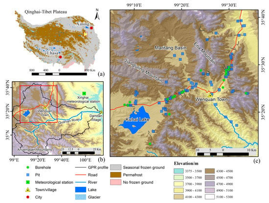
Figure 1.
(a) Location of the studied region on the Qinghai–Tibet Plateau; (b) the scope of the study area; (c) the topography of the investigated area with the locations of the field survey sites marked.
During the period from September to October 2009, a 30-day field investigation was conducted in the northern part of the catchment of the Qushian River. The field survey area is located between 35°15′–35°41′N latitude and 98°58′–99°43′E longitude, and its elevation ranges from 3562 to 5039 m, with an average altitude of more than 4000 m. The survey area has two mountains, named Erla Mountain and Jiangluling Mountain, and Kuhai Lake, which is a saltwater lake (Figure 1c).
The study area has a cool temperate continental climate. According to the monitoring of the Xinghai meteorological station (3535 m a.s.l) closest to the regional boundary (its location is marked in Figure 1b), the annual mean air temperature was 2.0 °C with a standard deviation of ±0.3 °C, and the annual precipitation was 200–370 mm during the period of 2003–2012. The flood season is from June to September, when the runoff accounts for about 70% of the total annual runoff. Precipitation in the flood season mostly occurs in the form of heavy rain or rainstorm, which often leads to flash floods in the mountain areas. Snow is the main form of precipitation in winter (from October to March), and the runoff generated in winter accounts for approximately 18% of the annual runoff. The vegetation types of the mountain areas are alpine meadow and swamp meadow, with the dominant plant being alpine Kobresia. Around Kuhai Lake at a relatively low altitude, there is an alpine steppe with Stipa purpurea as the dominant plant. The main soil type is silty loam, usually with gravels distributed on the surface.
2.2. Method and Data
2.2.1. GPR
The information on the permafrost boundary was obtained in three steps using GPR in this project.
- (1)
- Field survey and GPR data acquisition
Two methods were used to obtain the GPR data in this project: (1) the wide-angle reflection and refraction (WARR); and (2) the common-offset reflection (COR) method [30,31,41]. The WARR method is mainly used to detect the propagation velocity of electromagnetic waves and then determine the depth of the permafrost table, which is the key feature of GPR data interpretation. The COR method is used to detect the vertical and horizontal variations of a subsurface stratigraphic structure, especially to reflect the abnormal electromagnetic reflection signal due to the appearance or disappearance of permafrost in the horizontal direction as much as possible.
The equipment used for the field survey was a Professional Explorer (ProEx) GPR system (produced by Mala Corporation, Skolgatan, Sweden) with a rough terrain antenna (RTA) and unshielded antenna (UA). The central frequencies of the antennas are both 100 MHz. The RTA has the characteristics of a strong terrain coupling capability and high data acquisition efficiency and is especially suitable for mountainous environments, but it can only be used to perform COR survey tasks due to its fixed antenna offset. The UA has good anti-interference ability, and its transmitter and receiver can be separated, so it can perform both COR and WARR survey tasks. In the field investigation, we mainly used it to perform WARR tasks to determine the wave velocity at a specific location. When surveying with the RTA, we used a handheld GPS for positioning (Garmin Map60CS with a positioning accuracy of less than 15 m, produced by UniStrong Corporation, Beijing, China), and when working with the UA, a tape was used for the ground distance measurements. In the process of the survey, the change in surface conditions and their corresponding GPR track numbers needed to be recorded, especially for the COR profiles. Figure 2 shows the GPR profiles acquired with the UTA and UA, respectively. The same parameter settings were used for other profiles in this survey.

Figure 2.
The ground-penetrating radar (GPR) profiles obtained using different antennas and methods. (a) A GPR profile obtained by RTA (P034, altitude: 4309–4286 m, antenna offset: 2.2 m, sampling interval: 0.5 m). (b) A GPR profile acquired by unshielded antenna (UA), in which the common-offset reflection method (COR) was adopted for 0–40 m (antenna offset: 1 m, sampling interval: 0.1 m), and the wide-angle reflection and refraction (WARR) method was adopted after 40 m (sampling interval: 0.1 m). The velocities of the direct air wave, direct ground wave, and the reflected wave from the permafrost table can be calculated through the geometrical method on the WARR profile [41]. Profile (b) is located near the starting position of profile (a), and the borehole marked in the subgraphs is the same. The borehole provided information on the detailed stratigraphic structure, and its bottom temperature (at 10 m) was approximately −0.6 °C according to the measurement in November 2010, which indicates that the potential boundary of permafrost is probably close. The summary ground information is marked below the profile. Figure A1 provides more information on P034.
In the work, the layouts of the GPR profiles were designed according to the following principles: (1) these profiles should reflect the change of altitude; (2) they should cover different ASPs and cross different underlying surface types as far as possible. A total of 128 GPR profiles were deployed, most of which were longer than 500 m, and the longest profile reached ~3 km (Table A1). The altitude range of the GPR profiles is between 3900 m and 4700 m (Figure 3). The GPR survey was carried out from September to October of 2009, when the thickness of the active layer was close to the annual maximum, and the ground surface had not begun to freeze yet.
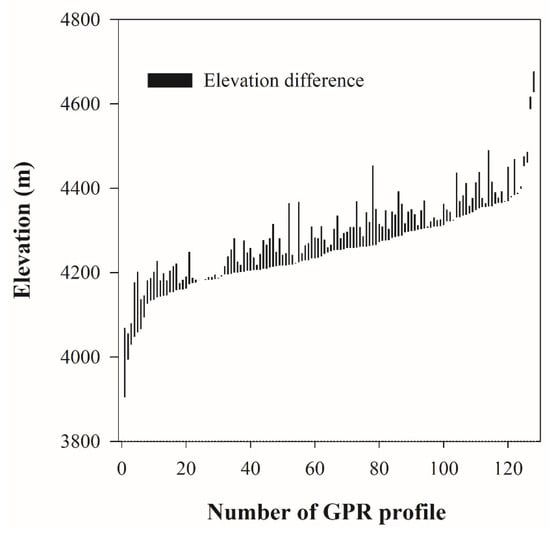
Figure 3.
The elevation ranges of ground-penetrating radar (GPR) profiles (arranged by the minimum altitude of each survey profile from low to high).
- (2)
- GPR data processing
In order to enhance deep signals and filter interference information on the GPR profiles, GPR data processing was necessary. This included the following steps: (1) subtract mean for the correction of signal saturation; (2) static correction for the adjustment of the time-zero position; (3) energy decay for the gain of signals; (4) background removal for the filtering of the horizontal signal; (5) band-pass filtering for the removal of specific frequency bands; (6) running average for the filtering of high-frequency noise signals; and (7) topographic correction. Among them, some are optional [30]. These steps are commonly used in GPR data processing for different targets, and the principles for their adoption are summarized in Neal’s report [31]. The processing was done using Reflexw software (Germany, introduced by http://www.sandmeier-geo.de/reflexw.html, accessed on 20 December 2021).
- (3)
- GPR data Interpretation
The interpretation of GPR data is the process of extracting permafrost information based on a variety of reference data. Firstly, the stratigraphic profiles from boreholes or pits that provide information on permafrost existence, soil texture, structure, etc. are the most important reference. Secondly, the change of the environmental factor in each profile, including the altitude, ASP, vegetation, landform, etc., is also considered. Google Earth, which provides a 3D visualization of remote sensing imagery, is a useful tool to aid in the interpretation of GPR data. Thirdly, the comparison and analogy of reflection features in different profiles are also the basis of interpretation.
The setting of the wave velocity follows the following principles: (1) the use of a wave velocity measured by WARR as mentioned above; (2) the use of a reverse-calculated wave velocity based on the depth of the permafrost table from a borehole or pit in or near the GPR profile; (3) the assignment of an empirical value derived from the wave velocity obtained by the above two methods according to the similarity of vegetation or micro-topography. Figure 4 and Figure 5 show several typical GPR profiles and their interpretation as examples, respectively, and Figure A1 gives more detailed information on these profiles and their display in Google Earth.
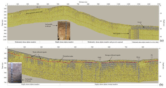
Figure 4.
Comparison of ground-penetrating radar (GPR) images between permafrost and seasonal frozen ground. (a) A typical seasonal frozen ground profile (P029, altitude: 3993–4093 m). The reflected signals are weak at 0–1200 m in the image. There is a uniform formation made up of sandy loam and no permafrost here, which is proved by a pit. The upper part of the soil profile in this pit is wet, and the lower part is dry. The latter half of the GPR image (after 1200 m) has strong reflected signals, but their continuity is poor. Considering that it is located in a river valley, these signals are interpreted as gravels brought by river alluvium. (b) A typical permafrost profile (P041, altitude: 4578–4617 m). In the profile, there is a continuous and clear in-phase reflection axis, which represents the existence of the permafrost table. The soil profile of a pit shows that the permafrost has high ice content and is located below a 1.2 m depth. According to this depth and the position of the reflection axis, the adopted wave velocity can be estimated. The ground temperature (at 10 m) observed in an adjacent borehole was approximately −2.5 °C in November 2010.
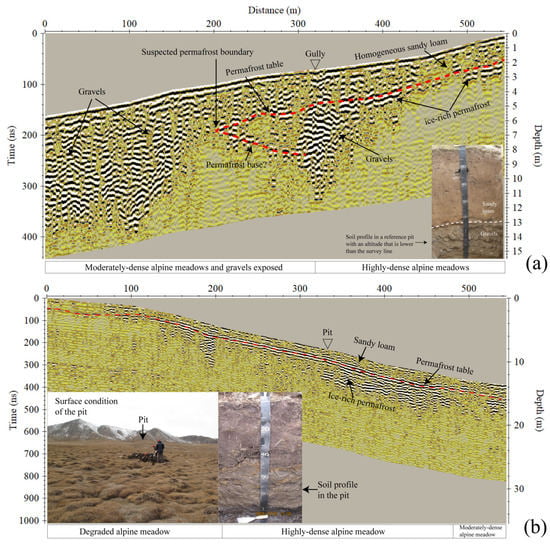
Figure 5.
The interpretation of two ground-penetrating radar (GPR) profiles in the same geomorphic unit. (a) P057 (altitude: 4125–4182 m), (b) P052 (altitude: 4264–4351 m). The first section (0–200 m) of P057 is mainly made up of gravels at a certain depth below the surface, and its interpretation depends on the soil profile in the pit that is close but lower than the start of the GPR profile (Figure A1b). After 200 m, there is an obvious continuous in-phase reflection axis, which is interpreted as the permafrost table. No wave velocity measurement was made here. The velocity setting of this profile was determined by referring to P052, which was deployed in the same geomorphic unit with similar vegetation and micro-geomorphic types. The wave velocity of the P052 has been determined as 0.07 m/ns according to a pit located in the middle of the survey line.
2.2.2. Boreholes and Pits
During the field investigation, 21 boreholes were deployed to detect permafrost and at 10 of which the ground temperatures were measured (~1 year after drilling) using thermistor temperature probes with an accuracy of ±0.05 °C (produced by the State Key Laboratory of Frozen Soil Engineering, Chinese Academy of Sciences). The rest of the boreholes were only used for the verification of the geophysical exploration, which helped to assess whether the permafrost existor not. At the same time, a number of pits were excavated, 39 of which were used as references for assessing the absence or presence of permafrost. In total, 60 ground truths from these boreholes and pits constitute a validation dataset. Among all these sites, 57 sites have definite records of vegetation types. In addition, we also collected soil samples from 13 pits and measured the soil volume moisture content by an oven-drying method in the laboratory. Then, the depth-weighted average moisture content within 1 m below the ground surface was calculated.
2.2.3. Spatial Data Products
The digital elevation model (DEM) used in this project was the ASTER GDEM V2 product with a spatial resolution of 30 m, which was produced by METI in Japan and NASA in the United States (downloaded from the Geospatial Data Cloud platform, http://www.gscloud.cn, accessed on 15 July 2021). The DEM data were used to calculate the topographic factors and estimate the potential incident solar radiation using ArcGIS software. For the analysis of the land surface temperature, MODIS LST products from 2003 to 2012, corrected by the method referred to in the literature [18], were adopted for the calculation of the multi-year average. The monthly air temperature data were extracted from the spatial dataset produced and corrected by Peng et al. [46] to calculate the multi-year mean air temperatures (downloaded from the Loess Plateau Science Data Center, National Earth System Science Data Sharing Infrastructure, National Science and Technology Infrastructure of China, http://loess.geodata.cn, accessed on 12 September 2021).
3. Results
3.1. Interpreted Results of GPR Profiles
The distribution of permafrost in mountainous areas is often fragmental and patchy due to the topographic impact (such as gullies formed by flowing water) and the complexity of the underlying surface. In the marginal areas of permafrost regions, the disappearance of permafrost is often abrupt; that is, permafrost disappears within a short horizontal distance. Some studies have shown that the depth of the permafrost table will increase considerably within a distance of less than 50 m near the edge of the permafrost region, and the frozen layer will quickly be pinched out [34,35], which generally occurs in the transition zone between continuous permafrost and seasonally frozen ground. When the GPR captures the horizontal variation in electromagnetic signals, it is possible to decipher information on the permafrost boundary from it.
GPR profiles generally pass through pits or boreholes that provide a reference basis for the interpretation of GPR data. In GPR images, strong and continuous in-phase reflection signals appear near the upper limit of permafrost (a depth range of 1.5–3.5 m in the study area, confirmed by pits or boreholes), often indicating the existence of permafrost. Thus, the main basis for assessing the boundary of permafrost patches is generally the interruption or disappearance of in-phase reflection signals that represent the permafrost table in the GPR images (Figure 2a and Figure 5a). In Section 2.2.1, the method of GPR profile interpretation is described in detail. Due to the uncertainty in the visual interpretation results of GPR, the extracted permafrost patch boundary is also called the suspected permafrost boundary (SPB). According to the GPS records during the field investigation using GPR, the geographic location and altitude of the permafrost patch boundary can be obtained. In total, 63 SPBs were identified and extracted from 128 GPR profiles (Table A1). For the rest of the profiles, some were entirely in the permafrost or seasonal frozen ground regions (e.g., the profiles in Figure 4), and the others were not easily interpreted due to a dry soil layer, excessive gravels, an insufficient detection depth of GPR, etc.
By analyzing the elevation of the SPBs, it was found that the most frequent occurrence of the SPB was between 4150 and 4350 m (Figure 6a), which indicates that this is the area where permafrost fragmentation and patches occur most frequently, as well as the transition zone from permafrost to seasonally frozen ground in the mountain permafrost region. The distribution of SPBs at different altitude zones is approximately normal. At the same time, the SPB also shows significant differences with different slope orientations. The statistical value of the south-facing slope is the largest, whereas the one of the north-facing slope is the smallest (Figure 6b). We plotted the lower limit of the permafrost along with the slope orientations in a polar coordinate system and found it can be regarded as a function of ASP (Figure 6c), which provides inspiration for improving the classical knowledge of permafrost distribution in mountainous permafrost.
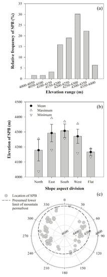
Figure 6.
(a) The frequency of the suspected permafrost boundary (SPB) occurring in different altitude zones; (b) the distribution of the elevations of the SPB at different aspects (ASPs); (c) the distribution of the SPB in a polar coordinate system, where the scale on the horizontal axis represents the elevation (m) and the angle represents the slope’s orientation (degree).
3.2. Construction of an Empirical–Statistical Model of Permafrost Distribution
The slope’s facing has an impact on the thermal state of the ground by influencing the solar radiation, atmospheric convection, and heat conduction, which eventually affects the existence of permafrost on a local or larger scale. There have been several traditional understandings of the permafrost zoning in mountainous areas under the influence of ASP [5,37,47]. Among them, the permafrost zoning scheme based on the ASP that was proposed by King had a profound impact: the highest elevation without permafrost developing on the south-facing slope is defined as the lower limit of continuous permafrost, and the lowest elevation with permafrost existing on the north-facing slope is defined as the lower limit of discontinuous permafrost (Figure 7). The two boundaries divide mountain permafrost into continuous, discontinuous, and sporadic/seasonal frozen ground from high to low altitude, and the altitude of each lower limit was generally treated as a fixed value in a local region rather than as a function of ASP, possibly due to the difficulty of detection and lack of data. The distribution map of the frozen ground produced based on this principle may cause trouble for users, such as underestimating the area of continuous permafrost or seasonally frozen ground or overestimating the area of discontinuous permafrost.
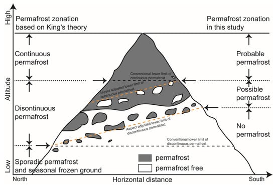
Figure 7.
Comparison between the conceptual models of mountain frozen ground zonation based on King’s theory and this research. The illustration was drawn with reference to French’s works [47] and the literature [5,37]. The left side of the graph illustrates the classical conceptual model of mountain permafrost zonation, and the right side shows the development made in this work based on classical theory. The orange dashed lines present adjustments of the lower limit of continuous and discontinuous permafrost under the influence of ASP.
According to the possibility of permafrost occurrence, the permafrost boundary or patch boundary can be detected by GPR mainly in the discontinuous permafrost belt. Thus, the closer the GPR profile’s location is to the upper continuous permafrost zone or to the lower seasonal frozen ground zone, the less likely it is to detect permafrost patch boundaries successfully, which is proved by the interpretation results of the GPR data (Figure 6a,c). Clearly, the possibility of the suspected permafrost patch boundary detected by GPR is affected by the ASP (Figure 6c), resulting in a new conceptual model of the mountain permafrost zonation presented (Figure 7).
In the new zonation scheme, the concept of “probable permafrost/possible permafrost/no permafrost” can be considered geographically equivalent to that of “continuous permafrost/discontinuous permafrost/sporadic permafrost and seasonal frozen ground” in King’s classical theory. The extent of the discontinuous permafrost zone becomes “narrow” and is regulated by the ASP, and the probabilities of the occurrence of permafrost and seasonally frozen ground, respectively, account for 50% in theory.
In this work, the layouts of the GPR profiles fully considered the influence of altitude and ASP, and relatively sufficient data were obtained (Figure 6a,c), providing the basis for building a statistical model. Based on the results from the GPR image interpretation, the relationship between the elevations of the permafrost patch boundary and the slope orientations can be described by a periodic function (Figure 8). The curve-fitting method was used to establish a mathematical model between the two indicators, and the model parameters were estimated. The form and parameters of the model are as follows:
where x is the slope orientation (degree), and y is the elevation of the SPB (m). The parameters obtained by curve fitting were: a = 91.7181, b = 4.8306, c = 4272.9235, R2 = 0.5212, and p < 0.0001. The p value indicates that the result is significant.
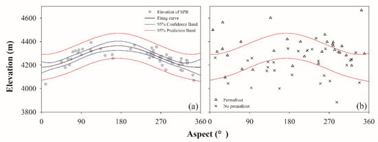
Figure 8.
(a) The curve fitting between elevations of the suspected permafrost boundary (SPB) and the slope orientations based on the interpretation results of the ground-penetrating radar (GPR) profiles; (b) the curve of the upper and lower limits of the prediction interval and the information of the field survey sites.
By comparing the field investigation of the pits and boreholes, it was found that a 95% prediction interval is ideal for describing the possible permafrost zone, and its upper and lower limits are in good agreement with the ground truths (Figure 8b). The upper and lower limits of the prediction interval ( and ) can be expressed by the following formula:
where is an unbiased estimate of the conditional mean when , n is the number of samples, is a critical value in the Student’s t distribution for degrees of freedom at a given confidence coefficient , is the sample variance, is the sample mean, and is a sample of the population. Mathematically, a prediction interval is a range of values that is likely to contain the value of a single new observation given the specified settings of the predictors, and a detailed explanation of the prediction interval is given in the work by [48]. When the confidence interval is 95%, the value of α is 0.05, and there is a 95% probability that the predicted value will be in the interval.
Thus, the complete model can be described by the following formulas:
where p = 1 represents probable permafrost, p = 0 represents possible permafrost, and p = −1 represents no permafrost. H0 is the actual altitude of the observation site. Figure 7 illustrates this empirical statistical model.
In this model, a 95% prediction interval indicates that the SPB has a 95% probability of falling within the prediction interval. In space, this area represents the transition zone from the permafrost to seasonally frozen ground, which corresponds to the discontinuous permafrost in King’s theory. Above the upper limit of the prediction interval, only a 5% probability is seasonally frozen soil theoretically, which is classified as probably permafrost, corresponding to continuous permafrost; below the lower limit of the prediction interval, only a 5% probability is permafrost, which is classified as no permafrost and corresponds to sporadic permafrost and seasonally frozen ground.
3.3. Model-Based Spatial Mapping and Evaluation
3.3.1. Frozen Ground Mapping by the Proposed Method
Based on the established empirical–statistical model, the spatial distribution of frozen ground in the study area was mapped using DEM and ASP data. According to the possibility of occurrence of permafrost patch boundaries, this map divides the frozen ground into three zones (probable permafrost zone, possible permafrost zone, and no permafrost zone) (Figure 9a).
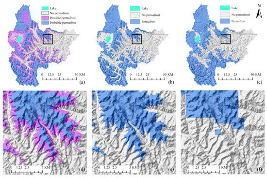
Figure 9.
Maps of frozen ground distribution in the study area. (a) Our method; (b) map based on Nan’s model in 2002; (c) map produced by Zou in 2017; (d–f) enlarged views of the three different maps, respectively.
3.3.2. Map Evaluation and Comparison with Two Existing Permafrost Maps
In order to evaluate the proposed new map (Figure 9a), a comparison was made with two existing maps. The first map was produced based on Nan’s model (referred to as Nan’s map). Nan et al. established a multiple regression model that only considers the altitude and latitude using limited ground temperature measurement data from boreholes located along the Qinghai–Tibet highway [21]. This model is generally considered to be one of the founders of the empirical–statistical model that later emerged to describe the distribution of permafrost in the Qinghai–Tibet Plateau. The expression of the model is as follows:
where is the mean annual ground temperature near the depth of zero annual amplitude, is the latitude, and is the elevation. = 0.5 °C is the boundary to determine the existence of permafrost. This model was applied to map the permafrost distribution using the same DEM data as the proposed new map in this study (Figure 9b).
The second one is Zou’s permafrost map (referred to as Zou’s map), which was produced based on the MODIS land surface temperature and TTOP model. It is the latest permafrost distribution map of the Qinghai–Tibet plateau, with a spatial resolution of 1 km, and it was well verified by the field-measured data [18] (Figure 9c).
For the entire area, the three maps can accurately reflect the distribution of permafrost, although there are differences among them in detail. These differences occur mainly in small basins with relatively flat terrain, such as the Kuhai Lake basin and the Maritang basin. The field investigation showed that both permafrost (mean annual ground temperature range of −0.7 to −2.2 °C at ~4170 m) and non-permafrost (mean annual ground temperature of 0.03 °C at ~4200 m) areas exist at the Kuhai Lake basin. However, at the bottom of the Maritang basin, there is uncertainty about the existence of permafrost. Three shallow pits with a maximum depth of 1.5 m have been dug in this area, and no permafrost has been found. Neither Nan’s map nor Zou’s map reflects the observation facts above, but the map produced in this work can depict this well. Furthermore, on the slopes of the mountains, the possible permafrost zone is distributed around the probable permafrost zone in a skirt shape. Moreover, it can be reflected in detail that the distribution of the permafrost zone is affected by the ASP (Figure 9d–f). Therefore, the permafrost zoning map is consistent with the actual field survey results and theoretical analysis and has better rationality in describing the possibility of permafrost existence in mountainous areas.
However, most of the existing permafrost distribution maps with different spatial scales of the QTP, represented by the above two maps, only provide a binary classification of permafrost occurrence (with or without permafrost). The limited pit or borehole surveys also only provide binary information on the presence or absence of permafrost.
In order to evaluate the performance of the ternary classification map produced by this study, we proposed a method to calculate the agreement (consistency) between our ternary classification map and the binary maps or ground truths (Table 1). By comparing the binary classification map and the ternary classification map, it was found that the possible permafrost type that corresponds to the discontinuous permafrost zone is the key to evaluating the performance of cartography. The consistency calculation is based on the assumption that the probability of both permafrost and non-permafrost occurrence is 50% in the possible permafrost zone in the new map of frozen ground. For the calculation of the consistency of the whole map, the area weighting method was adopted, and the proportions of different zones to the total area were taken as the weight of the spatial evaluation (Table 1).

Table 1.
The comparison scheme of evaluating consistency between our ternary mapping results and the existing binary maps/field survey dataset.
Then, the new permafrost zonation map was compared with two existing frozen ground maps, and its agreements with the existing maps and field survey ground truths were analyzed, with consistency as an indicator (Table 2). The coincidence degree between Nan’s map and the proposed permafrost zone map in this study was up to 97.7% (Table 2), whereas that between Zou’s map and the new map reached 81.8%. However, for areas that belong to the possible permafrost zone, the consistency between the two maps was only 58.2% (Table 2) because 70% of this zone is considered to be permafrost in Zou’s map, probably due to its lower resolution of 1 km. There are 60 pits or boreholes located in the field survey area (Figure 1), which provide evidence of the presence or absence of permafrost as ground truth (Figure 8b). They were also used to test the consistency between the permafrost zoning map and the real situation. The coincidence degrees between the three frozen ground zones and the ground truth reached 87.5%, 96.3%, and 82.4%, respectively. The weighted average of the entire region was 87.8% (Table 2). In general, the new permafrost zonation map performs well.

Table 2.
The areas and proportions of different permafrost zones based on the mapping results, as well as their consistency with existing maps and ground truth from survey field sites.
3.4. Temperature Characteristics at the Boundaries between Different Frozen Ground Zones
According to the above study, there are two invisible boundaries between the mountain permafrost sub-zones, which distinguish continuous permafrost zone, discontinuous permafrost zone, and sporadic and seasonal frozen ground zone. Approximately 1200 samples were selected from the two boundaries, and their multi-year average temperatures and ground temperatures during the period of 2003 to 2012 were calculated and are shown in boxplots in Figure 10. At the two boundaries, both the air temperature and land surface temperature have wide ranges of values and show the characteristics of approximate normal distribution. The lower limit of the discontinuous permafrost distribution (LLD) corresponds to the multi-year mean land surface temperature of 0.3 °C (standard deviation of ±1.0 °C) and the multi-year mean air temperature of −3.9 °C (standard deviation ±0.9 °C). The lower limit of the continuous permafrost (LLC) distribution corresponds to the multi-year mean land surface temperature of −1.3 °C (standard deviation of ±1.3 °C) and the multi-year mean air temperature of −5.7 °C (standard deviation of ±1.1 °C). King reported that the mean annual air temperature of −4 °C indicated the regional lower limit of the discontinuous permafrost zone in high-latitude mountains [5]. This is consistent with this study (−3.9 °C), although the air temperatures extracted from reanalysis data with a coarse grid have large uncertainties at a local scale [46].
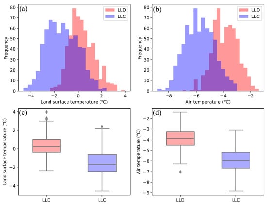
Figure 10.
Statistics of land surface temperature and temperature at the lower limits of continuous permafrost and discontinuous permafrost. (a,c) show the data frequency and box plots of the land surface temperature at the lower limit of continuous permafrost (LLC) and the lower limit of discontinuous permafrost distribution (LLD), respectively. (b,d) show the data frequency and box plots of the air temperature at the LLC and LLD, respectively.
3.5. Vegetation Types in Different Zones of Frozen Ground
The vegetation types of the field sites in the different frozen ground zones were analyzed (Table 3). In the zone of no permafrost, most of the sites are covered by alpine steppe with relatively sparse vegetation, and in most sites where alpine meadow and alpine swamp meadow developed, permafrost was not found. The only exceptions were three sites around Kuhai Lake, where permafrost was found. These three sites are located on seasonal wetlands, the formation of which is related to the terrain around Kuhai Lake. All the sites with swamp meadow in the discontinuous permafrost zone have permafrost, and the sites with alpine steppe have the lowest possibility of permafrost developing. Overall, the possibility of permafrost occurrence in continuous permafrost or discontinuous permafrost, from high to low, is alpine swamp meadow (ASM) > alpine meadow (AM) > alpine steppe (AS).

Table 3.
Statistics of field survey sites for different vegetation types and permafrost existence in different frozen ground zones. ASM, AM, and AS represent alpine swamp meadow, alpine meadow, and alpine steppe, respectively.
In this project, special attention was paid to the discontinuous permafrost belt because the spatial variability of vegetation in this region may be more controlled by local hydro-thermal conditions rather than altitude and ASP. The vegetation type is generally a reflection of moisture conditions. The average soil water content data from a limited number of boreholes or pits located in the possible permafrost zone in the new map were extracted and analyzed. The results show that the soil water content of all sites with permafrost present is relatively high except for only one site, and the water content of the eight sites without permafrost is less than or equal to 25% (Figure 11). Based on the existing observations, it can be inferred that 25% may be an average soil moisture threshold determining the existence of permafrost, at least for most cases. It also partly explains why sites with good vegetation conditions tend to have a higher probability of permafrost occurrence.
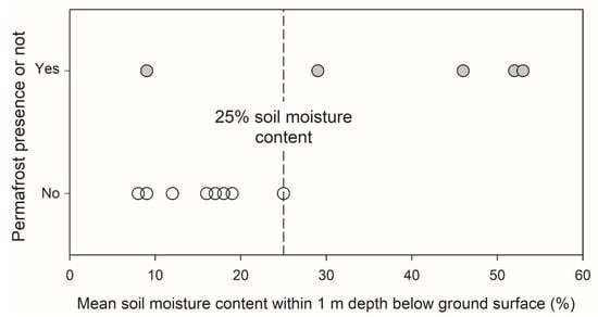
Figure 11.
The existence of permafrost under different mean soil moisture content conditions.
4. Discussion
4.1. The Influence of Solar Radiation on Permafrost in Mountainous Regions
Altitude and solar radiation play an important role in the development and distribution of mountain permafrost [26,27,49,50], and solar radiation is largely regulated by the slope direction in mountainous areas [6].
Using the GIS platform, the annual total potential incident solar radiation on different ASPs and altitude zones were calculated and are shown in Figure 12a. In general, the value of the potential incident solar radiation increased as the altitude increased. At the same altitude zone, the potential incident solar radiation values of sunny slopes were significantly greater than those of shady slopes, and the maximum value appeared on the southwest-facing slope. Therefore, compared to the shady slopes, the lower limits of permafrost distribution are higher on the sunny slopes.
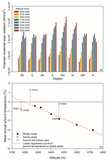
Figure 12.
(a) Distribution of annual potential incident solar radiation at different aspects of the slope at different altitude zones; (b) differences in annual mean ground temperature observed from different borehole sites.
The ground temperatures measured from the boreholes in the field also revealed the influence of ASP on the thermal regime of permafrost. Figure 12b shows that the ground temperatures at a depth of 10 m on the sunny slope were higher than those on the shady slope by 1.4–1.6 °C at the same altitude. This difference between sunny and shady slopes was also revealed in other mountain areas. For example, the ground temperature difference between sunny and shady slopes in the Fenghuoshan Mountain in the hinterland of the QTP is 1.7–2.4 °C where abundant ground ice exists [51], whereas the differences reached 1.0–6.0 °C in the Tienshan Mountains, with higher latitudes and steeper slopes [52]. The reason for the small temperature difference between sunny and shady slopes in this area may be because the slopes where borehole sites are located are relatively gentle. In addition, the two boreholes (WQ01 and WQ02) located in the Kuhai Lake basin are special, and the ground temperature is 0.8–1.0 °C lower than that of the shady slope of the mountain region at the same altitude. Through the analysis of the surface conditions and core descriptions of the boreholes, it was determined that the two sites are located on seasonal wetlands with relatively flat terrain, and the existence of permafrost at these locations is mainly due to the influence of rich soil moisture content rather than ASP.
4.2. Significance and Limitation of this Model Based on GPR Data
The influence of ASP on permafrost can be verified and simulated using theoretical models [53], but it is difficult to observe directly and describe quantitatively. Some previous studies have shown that ground temperature can reflect the difference between shady slopes and sunny slopes to a certain extent [54]. However, there can still be great uncertainty in quantifying the impact of shady and sunny slopes from the perspective of ground temperature unless strict control conditions are adopted. Sometimes, periglacial geomorphic features on landscapes are used as alternative indicators to determine the lower limit of mountain permafrost, such as rock glaciers [55]. However, for areas with less steep terrain or insufficiently low temperatures, the typical periglacial phenomena may be very limited, such as the area of concern in this case.
This work used GPR as a field observation method to reveal the influence of ASP on the distribution of permafrost for the first time in a mountain region of the Qinghai–Tibet Plateau. The established zoning model of permafrost distribution in mountainous areas considering the adjustment of ASP is an improvement and supplement to King’s theory. However, it cannot distinguish between permafrost and no permafrost well, considering the characteristics of fragmentation and patches of permafrost in discontinuous permafrost belts and transient zones, where the permafrost development is affected by soil texture, soil moisture, vegetation cover, etc. comprehensively.
Although this model was developed in a local area, the law regarding the influence of ASP on permafrost distribution revealed that it can be referenced by other studies that involve mountain permafrost regions. In addition, the map of frozen ground, taking into account the ASP adjustment in this study, describes the distribution characteristics of mountain permafrost in detail, especially distinguishing the transition zone between permafrost and no permafrost. The permafrost in this zone is generally more sensitive to climate change and may degrade first under climate warming, bringing higher geological and engineering risks [26]. The permafrost mapping result of this work has a wide range of applicability in studying the differences in vegetation evolution and hydrological processes in different permafrost zones, as well as the occurrence of permafrost-related disasters.
GPR has a wide range of applications in the detection of sedimentary structures in permafrost regions, which mainly focus on the interpretation of vertical permafrost features [30,36,37,40,43,44,45]. When studying the spatial distribution of permafrost, GPR data can be regarded as a data source participating in statistical or machine learning models that are generally based on a large amount of data and support multivariate environmental data [22,23,24,25,32,49]. The participation of data with multiple scales and qualities will bring more uncertainty to the assessment of permafrost distribution and will also greatly increase the cost of resources and time. In this context, this project puts forward a new method of GPR application, which uses the horizontal abnormalities of electromagnetic signals recorded by GPR. It makes it possible to quickly build a distribution model of frozen ground relying on only GPR data and DEM. Obviously, this model is more efficient and easier to interpret.
However, a limitation is that the proposed permafrost mapping scheme has high requirements for the layout of the GPR profiles: (1) the GPR profiles need to reflect the variations in altitude and ASP as much as possible; (2) the GPR profiles should cross the possible boundaries of permafrost patches as much as possible, which are often marked by the transformation of the landscape; for example, the GPR profile can pass through from alpine meadow to alpine steppe; (3) a sufficient number of GPR profiles are necessary in order to obtain a statistical law. In order to guarantee the sufficiency of the survey, an empirical estimation is that at least 5–10 effective GPR profiles should be deployed on each slope’s facing (reclassified as east, south, west, and north).
5. Conclusions
In this project, GPR was used to survey the permafrost boundary in the mountainous area of the Qinghai–Tibet Plateau, and the interpretation results of the GPR profiles were used to establish a permafrost zoning model at a regional scale for the first time. It was proved that the GPR method has good applicability in the detection and mapping of permafrost in the mountainous areas with rugged terrain on the QTP.
The mountain permafrost zoning model, taking into account the ASP established by GPR, depicted the distribution of permafrost in the mountain area in detail and revealed that the area proportions of continuous permafrost, discontinuous permafrost, and seasonal permafrost in the region were 38.1%, 25.0%, and 36.9%, respectively. The LLC was 4472 m on the sunny slope and 4291 m on the shady slope, and the multi-year average land surface temperature and air temperature were −1.3 °C and −5.7 °C, respectively, near the boundary between the continuous permafrost zone and the discontinuous permafrost zone. Meanwhile, the LLD was 4258 m on the sunny slope and 4061 m on the shady slope, and the multi-year average land surface temperature and air temperature were −0.3 °C and −3.9 °C, respectively, near the boundary between the discontinuous permafrost zone and the no permafrost zone.
In mountainous regions, altitude leads to the vertical zonation of permafrost, and ASP regulates the distribution of permafrost by modulating the incoming solar radiation. The influence of ASP on the lower limit altitude of continuous and discontinuous permafrost is approximately 180–200 m. Thermal regime observations showed that the ground temperature on the sunny slope was 1.4–1.6 °C higher than that on the shady slope at the same altitude. However, in addition to the ASP, there are other local factors in this area. For example, the ground temperature of permafrost in the seasonal wetland near Kuhai Lake was 0.8–1.0 °C lower than that on the shady slope in mountain areas.
The elevation range of the discontinuous permafrost zone was 200–240 m on the vertical projection plane. The discontinuous permafrost zone is located on the outskirts of the continuous permafrost zone in the mountainous areas, but in the relatively flat areas of the intermountain basin, the permafrost distribution is characterized by patches and fragmentation. In the discontinuous permafrost zone, the leading factor determining the permafrost presence or absence may be soil moisture, which can be indicated by vegetation conditions to some extent. According to the field measurements of soil moisture from 13 pits, a 25% soil water content (the mean volume content within 1 m below the surface) can be used as a threshold to assess the presence or absence of permafrost in the discontinuous permafrost zone.
Author Contributions
Conceptualization—ideas, G.L.; project administration, L.Z.; field investigation, G.L., L.Z., D.Z., E.D., Y.Z., Y.X. and Y.S.; methodology, G.L. and E.D.; data processing, G.L. Y.X. and E.D.; Resources, G.L., L.Z., C.X., T.W., E.D. and D.Z.; writing—original draft preparation, G.L.; writing—review and editing, G.L., C.X., T.W., L.W., L.Z., D.Z. and C.W.; literature arrangement, Y.W. All authors have read and agreed to the published version of the manuscript.
Funding
This research was funded by the Second Tibetan Plateau Scientific Expedition and Research Program (2019QZKK0201), State Key Laboratory of Cryospheric Science (SKLCS-ZZ-2022), National Natural Science Foundation of China (41931180, 42071094, 41671068), and Strategic Priority Research Program of the Chinese Academy of Sciences (XDA2002010202).
Data Availability Statement
The data presented in this study are available on request from the corresponding author.
Acknowledgments
Thanks for the guidance and contribution from Qihao Yu, Yanhui You, and Wu Wang, etc. in the field investigation. For the data processing and visualization in this project, we used the Anaconda platform (https://anaconda.org), Python programming language (https://www.python.org), SciPy (https://scipy.org), NumPy (https://numpy.org), pandas (https://pandas.pydata.org), and matplotlib (https://matplotlib.org) module.
Conflicts of Interest
The authors declare no conflict of interest.
Appendix A
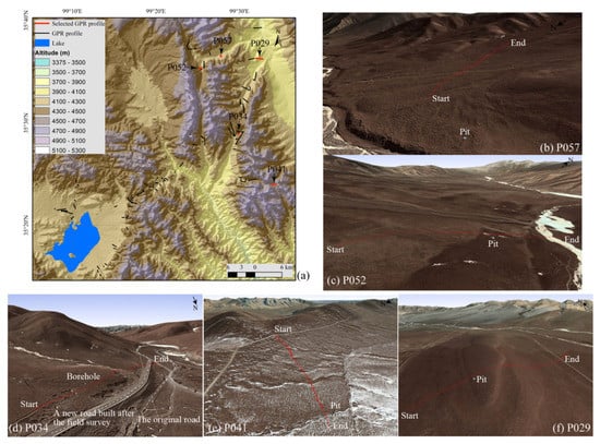
Figure A1.
(a) The locations of all GPR profiles involved in this article; (b–f) correspond to the GPR profiles P057, P052, P034, P041, and P029, which are displayed in Google Earth, respectively. When we carried out the GPR survey, the construction of the new road in the subgraph (d) had not started yet.

Table A1.
Inventory of the GPR profiles and corresponding elevations of SPB.
Table A1.
Inventory of the GPR profiles and corresponding elevations of SPB.
| ID of the GPR Profile | Start of the Survey Line | End of the Survey Line | Elevation of SPB (m) | ID of the GPR Profile | Start Of the Survey Line | End of the Survey Line | Elevation of SPB (m) | ||||
|---|---|---|---|---|---|---|---|---|---|---|---|
| Latitude (°N) | Longitude (°E) | Latitude (°N) | Longitude (°E) | Latitude (°N) | Longitude (°E) | Latitude (°N) | Longitude (°E) | ||||
| P001 | 35.4856 | 99.5094 | 35.4854 | 99.5034 | —— | P065 | 35.4795 | 99.4232 | 35.4746 | 99.4268 | 4336 |
| P002 | 35.4855 | 99.5023 | 35.4872 | 99.4954 | 4338 | P066 | 35.4753 | 99.4279 | 35.4761 | 99.4295 | —— |
| P003 | 35.4852 | 99.5077 | 35.4851 | 99.5072 | —— | P067 | 35.4762 | 99.4295 | 35.4700 | 99.4297 | 4270 |
| P004 | 35.4848 | 99.5057 | 35.4844 | 99.5056 | —— | P068 | 35.4690 | 99.4299 | 35.4696 | 99.4322 | —— |
| P005 | 35.3603 | 99.1728 | 35.3678 | 99.1688 | —— | P069 | 35.3459 | 99.2710 | 35.3459 | 99.2645 | —— |
| P006 | 35.3753 | 99.1704 | 35.3726 | 99.1725 | 4227 | P070 | 35.3444 | 99.2769 | 35.3457 | 99.2717 | —— |
| P007 | 35.3659 | 99.1703 | 35.3662 | 99.1701 | —— | P071 | 35.3490 | 99.2790 | 35.3456 | 99.2754 | 4355 |
| P008 | 35.3572 | 99.1450 | 25.3575 | 99.1449 | —— | P072 | 35.3462 | 99.2775 | 35.3468 | 99.2765 | 4354 |
| P009 | 35.3583 | 99.1453 | 35.3552 | 99.1449 | —— | P073 | 35.2951 | 99.2537 | 35.2960 | 99.2476 | 4244 |
| P010 | 35.3566 | 99.1449 | 35.3519 | 99.1684 | —— | P074 | 35.2667 | 99.2392 | 35.2677 | 99.2378 | —— |
| P011 | 35.3570 | 99.1561 | 35.3558 | 99.1556 | —— | P075 | 35.2684 | 99.2365 | 35.2711 | 99.2312 | 4217 |
| P012 | 35.3569 | 99.1560 | 35.3567 | 99.1441 | —— | P076 | 35.3655 | 99.2561 | 35.3629 | 99.2495 | —— |
| P013 | 35.4743 | 99.4959 | 35.4731 | 99.4925 | 4262 | P077 | 35.3261 | 99.2778 | 35.3308 | 99.2737 | —— |
| P014 | 35.4841 | 99.5071 | 35.4647 | 99.4915 | 4267 | P078 | 35.3637 | 99.2867 | 35.3630 | 99.2860 | —— |
| P015 | 35.4647 | 99.4915 | 35.4656 | 99.4972 | 4218 | P079 | 35.3630 | 99.2860 | 35.3635 | 99.2809 | —— |
| P016 | 35.4651 | 99.4956 | 35.4656 | 99.4974 | 4261 | P080 | 35.3635 | 99.2809 | 35.3635 | 99.2768 | —— |
| P017 | 35.4583 | 99.4873 | 35.4569 | 99.4932 | 4205 | P081 | 35.2503 | 99.2241 | 35.2538 | 99.2206 | 4257 |
| P018 | 35.5012 | 99.4818 | 35.4783 | 99.4915 | 4346 | P082 | 35.2558 | 99.2175 | 35.2613 | 99.2171 | —— |
| P019 | 35.4798 | 99.4899 | 35.4808 | 99.4914 | 4290 | P083 | 35.2617 | 99.2195 | 35.2672 | 99.2159 | 4237 |
| P020 | 35.5158 | 99.5099 | 35.5320 | 99.5075 | 4263 | P084 | 35.2649 | 99.2299 | 35.2675 | 99.2278 | 4234 |
| P021 | 35.5403 | 99.5074 | 35.5334 | 99.5182 | 4242 | P085 | 35.2977 | 99.2553 | 35.3017 | 99.2463 | —— |
| P022 | 35.5369 | 99.5120 | 35.5379 | 99.5100 | 4228 | P086 | 35.3460 | 99.1643 | 35.3423 | 99.1661 | —— |
| P023 | 35.5708 | 99.5268 | 35.5694 | 99.5312 | —— | P087 | 35.3452 | 99.1670 | 35.3475 | 99.1692 | —— |
| P024 | 35.5695 | 99.5308 | 35.5827 | 99.5345 | 4115 | P088 | 35.3583 | 99.1448 | 35.3555 | 99.1453 | 4180 |
| P024 | 35.5695 | 99.5308 | 35.5827 | 99.5345 | 4070 | P089 | 35.3555 | 99.1459 | 35.3584 | 99.1461 | 4180 |
| P025 | 35.5301 | 99.5025 | 35.5326 | 99.5030 | 4322 | P090 | 35.3563 | 99.1570 | 35.3574 | 99.1526 | 4181 |
| P026 | 35.5312 | 99.5019 | 35.5392 | 99.5017 | 4307 | P091 | 35.3580 | 99.1346 | 35.3602 | 99.1543 | 4188 |
| P027 | 35.6536 | 99.5281 | 35.6545 | 99.5450 | —— | P092 | 35.3585 | 99.1320 | 35.3611 | 99.1308 | —— |
| P028 | 35.6031 | 99.5177 | 35.6050 | 99.5314 | —— | P093 | 35.4077 | 99.1736 | 35.4030 | 99.1736 | —— |
| P029 | 35.6050 | 99.5320 | 35.6044 | 99.5479 | —— | P094 | 35.3977 | 99.1799 | 35.4001 | 99.1763 | —— |
| P030 | 35.5586 | 99.5052 | 35.5547 | 99.5170 | 4202 | P095 | 35.3777 | 99.2784 | 35.3733 | 99.2794 | —— |
| P031 | 35.5540 | 99.5165 | 35.5525 | 99.5222 | 4151 | P096 | 35.3692 | 99.2867 | 35.3732 | 99.2799 | —— |
| P032 | 35.5540 | 99.5218 | 35.5604 | 99.5201 | 4152 | P097 | 35.3776 | 99.2891 | 35.3771 | 99.2853 | 4323 |
| P033 | 35.4829 | 99.5002 | 35.4849 | 99.4982 | 4302 | P098 | 35.3796 | 99.2875 | 35.3802 | 99.2840 | 4339 |
| P034 | 35.4831 | 99.5001 | 35.4827 | 99.4994 | 4301 | P099 | 35.3767 | 99.2856 | 35.3727 | 99.2793 | —— |
| P035 | 35.4922 | 99.4768 | 35.4876 | 99.4820 | 4392 | P100 | 35.3784 | 99.2773 | 35.3770 | 99.2786 | —— |
| P036 | 35.4870 | 99.4818 | 35.4782 | 99.4901 | 4289 | P101 | 35.3817 | 99.2994 | 35.3813 | 99.2964 | —— |
| P037 | 35.4087 | 99.5129 | 35.4039 | 99.5118 | 4275 | P102 | 35.3864 | 99.2975 | 35.3816 | 99.2946 | 4370 |
| P038 | 35.4039 | 99.5119 | 35.4054 | 99.5028 | 4255 | P103 | 35.3684 | 99.2954 | 35.3731 | 99.2796 | 4295 |
| P039 | 35.4054 | 99.5028 | 35.4095 | 99.5033 | —— | P104 | 35.3735 | 99.2880 | 35.3735 | 99.2837 | —— |
| P040 | 35.4098 | 99.5033 | 35.4110 | 99.5052 | —— | P105 | 35.3918 | 99.3080 | 35.3896 | 99.3072 | —— |
| P041 | 35.4007 | 99.5738 | 35.3990 | 99.5638 | —— | P106 | 35.4361 | 99.3883 | 35.4287 | 99.3813 | —— |
| P042 | 35.4093 | 99.5339 | 35.4079 | 99.5281 | —— | P107 | 35.4111 | 99.3436 | 35.4095 | 99.3472 | —— |
| P043 | 35.4078 | 99.5275 | 35.4063 | 99.5170 | 4305 | P108 | 35.4119 | 99.3374 | 35.4094 | 99.3353 | —— |
| P044 | 35.4107 | 99.5036 | 35.4117 | 99.4978 | —— | P109 | 35.4063 | 99.3329 | 35.4078 | 99.3342 | 4228 |
| P045 | 35.4798 | 99.4009 | 35.4820 | 99.4029 | —— | P110 | 35.4030 | 99.3328 | 35.4017 | 99.3378 | —— |
| P046 | 35.6368 | 99.4004 | 35.6345 | 99.3994 | —— | P111 | 35.4019 | 99.3323 | 35.4015 | 99.3373 | —— |
| P047 | 35.6327 | 99.3996 | 35.6255 | 99.3951 | —— | P112 | 35.3974 | 99.3438 | 35.3979 | 99.3433 | —— |
| P048 | 35.6256 | 99.3952 | 35.6197 | 99.3975 | —— | P113 | 35.3990 | 99.3267 | 35.3966 | 99.3282 | 4257 |
| P049 | 35.6195 | 99.3972 | 35.6197 | 99.4065 | 4313 | P114 | 35.4025 | 99.3103 | 35.3982 | 99.3165 | 4329 |
| P050 | 35.6197 | 99.4088 | 35.6207 | 99.4154 | 4288 | P115 | 35.4194 | 99.3708 | 35.4223 | 99.3723 | 4038 |
| P051 | 35.5878 | 99.4262 | 35.5859 | 99.4200 | —— | P116 | 35.4069 | 99.3578 | 35.4084 | 99.3551 | —— |
| P052 | 35.5858 | 99.4199 | 35.5912 | 99.4247 | 4275 | P117 | 35.4084 | 99.3551 | 35.4085 | 99.3540 | 4200 |
| P053 | 35.5898 | 99.4267 | 35.5896 | 99.4296 | 4272 | P118 | 35.4085 | 99.3539 | 35.4096 | 99.3502 | —— |
| P054 | 35.5896 | 99.4296 | 35.6009 | 99.4291 | 4288 | P119 | 35.4045 | 99.3528 | 35.4080 | 99.3494 | 4159 |
| P055 | 35.6097 | 99.4416 | 35.6143 | 99.4407 | —— | P120 | 35.4033 | 99.3482 | 35.4094 | 99.3504 | 4133 |
| P056 | 35.6143 | 99.4403 | 35.6155 | 99.4396 | 4282 | P121 | 35.3979 | 99.3433 | 35.3990 | 99.3422 | —— |
| P057 | 35.6104 | 99.4609 | 35.6070 | 99.4649 | 4159 | P122 | 35.3990 | 99.3422 | 35.4005 | 99.3411 | 4199 |
| P058 | 35.4660 | 99.4070 | 35.4644 | 99.4075 | —— | P123 | 35.3990 | 99.3267 | 35.3966 | 99.3282 | —— |
| P059 | 35.4645 | 99.4076 | 35.4636 | 99.4138 | 4318 | P124 | 35.3938 | 99.3285 | 35.3957 | 99.3294 | 4251 |
| P060 | 35.4635 | 99.4139 | 35.4633 | 99.4155 | —— | P125 | 35.3892 | 99.3371 | 35.3926 | 99.3324 | 4233 |
| P061 | 35.4699 | 99.4252 | 35.4692 | 99.4282 | —— | P126 | 35.3957 | 99.3202 | 35.3958 | 99.3276 | 4252 |
| P062 | 35.4683 | 99.4299 | 35.4644 | 99.4308 | —— | P127 | 35.3871 | 99.3096 | 35.3896 | 99.3078 | —— |
| P063 | 35.4637 | 99.4311 | 35.4632 | 99.4324 | —— | P128 | 35.3901 | 99.3102 | 35.3831 | 99.2995 | —— |
| P064 | 35.4767 | 99.4266 | 35.4794 | 99.4235 | 4330 | ||||||
References
- Zhang, T.; Heginbottom, J.A.; Barry, R.G.; Brown, J. Further statistics on the distribution of permafrost and ground ice in the northern hemisphere. Polar Geogr. 2000, 24, 126–131. [Google Scholar] [CrossRef]
- Ran, Y.; Li, X.; Cheng, G.; Zhang, T.; Wu, Q.; Jin, H.; Jin, R. Distribution of permafrost in china: An overview of existing permafrost maps. Permafr. Periglac. Processes 2012, 23, 322–333. [Google Scholar] [CrossRef]
- Haeberli, W. Mountain permafrost—Research frontiers and a special long-term challenge. Cold Reg. Sci. Technol. 2013, 96, 71–76. [Google Scholar] [CrossRef]
- Zhao, L.; Zou, D.; Hu, G.; Du, E.; Pang, Q.; Xiao, Y.; Li, R.; Sheng, Y.; Wu, X.; Sun, Z.; et al. Changing climate and the permafrost environment on the Qinghai–Tibet (Xizang) Plateau. Permafr. Periglac. Processes 2020, 31, 396–405. [Google Scholar] [CrossRef]
- King, L. Zonation and ecology of high mountain permafrost in Scandinavia. Geogr. Ann. Ser. A Phys. Geogr. 1986, 68, 131–139. [Google Scholar] [CrossRef]
- Haeberli, W.; Noetzli, J.; Arenson, L.; Delaloye, R.; Gärtner-Roer, I.; Gruber, S.; Isaksen, K.; Kneisel, C.; Krautblatter, M.; Phillips, M. Mountain permafrost: Development and challenges of a young research field. J. Glaciol. 2011, 56, 1043–1058. [Google Scholar] [CrossRef] [Green Version]
- Cheng, G.; Dramis, F. Distribution of mountain permafrost and climate. Permafr. Periglac. Processes 1992, 3, 83–91. [Google Scholar]
- Zhang, G.; Yao, T.; Xie, H.; Qin, J.; Ye, Q. Estimating surface temperature changes of lakes in the Tibetan Plateau using modis lst data. J. Geophys. Res. 2014, 119, 8552–8567. [Google Scholar] [CrossRef]
- Field, C.B.; Barros, V.R. IPCC (2014) climate change 2014: Impacts, adaptation, and vulnerability. Part A: Global and sectoral aspects. In Contribution of Working Group II to the 5th Assessment Report of the Intergovernmental Panel on Climate Change; Cambridge University Press: Cambridge, UK, 2014; p. 1132. [Google Scholar]
- Wu, Q.; Zhang, T. Recent permafrost warming on the Qinghai-Tibetan Plateau. J. Geophys. Res. 2008, 113, D13108. [Google Scholar] [CrossRef]
- Zhao, L.; Zou, D.; Hu, G.; Wu, T.; Du, E.; Liu, G.; Xiao, Y.; Li, R.; Pang, Q.; Qiao, Y.; et al. A synthesis dataset of permafrost thermal state for the qinghai–tibet (xizang) plateau, China. Earth Syst. Sci. Data 2021, 13, 4207–4218. [Google Scholar] [CrossRef]
- Mollaret, C.; Hilbich, C.; Pellet, C.; Flores-Orozco, A.; Delaloye, R.; Hauck, C. Mountain permafrost degradation documented through a network of permanent electrical resistivity tomography sites. Cryosphere 2019, 13, 2557–2578. [Google Scholar] [CrossRef] [Green Version]
- Wang, G.; Yuanshou, L.I.; Qingbai, W.U.; Wang, Y. Impacts of permafrost changes on alpine ecosystem in Qinghai-Tibet Plateau. Sci. China Ser. D Earth Sci. 2006, 49, 1156–1169. [Google Scholar] [CrossRef]
- Yang, Z.; Gao, J.; Lin, Z.; Xu, X.; Ouyang, H. Linking thaw depth with soil moisture and plant community composition: Effects of permafrost degradation on alpine ecosystems on the Qinghai-Tibet Plateau. Plant Soil 2013, 367, 687–700. [Google Scholar] [CrossRef]
- Rogger, M.; Chirico, G.B.; Hausmann, H.; Krainer, K.; Brückl, E.; Stadler, P.; Blöschl, G. Impact of mountain permafrost on flow path and runoff response in a high alpine catchment. Water Resour. Res. 2017, 53, 1288–1308. [Google Scholar] [CrossRef] [Green Version]
- Patton, A.I.; Rathburn, S.R.; Capps, D.; Brown, R.A.; Singleton, J.S. Lithologic, geomorphic, and permafrost controls on recent landsliding in the Alaska range. Geosphere 2020, 16, 1479–1494. [Google Scholar] [CrossRef]
- Gruber, S.; Haeberli, W. Permafrost in steep bedrock slopes and its temperature-related destabilization following climate change. J. Geophys. Res. Earth Surf. 2007, 112, F02S18. [Google Scholar] [CrossRef] [Green Version]
- Zou, D.; Zhao, L.; Sheng, Y.; Chen, J.; Hu, G.; Wu, T.; Wu, J.; Xie, C.; Wu, X.; Pang, Q.; et al. A new map of permafrost distribution on the Tibetan Plateau. Cryosphere 2017, 11, 2527–2542. [Google Scholar] [CrossRef] [Green Version]
- Guo, D.; Wang, H. Simulation of permafrost and seasonally frozen ground conditions on the Tibetan Plateau, 1981–2010. J. Geophys. Res. Atmos. 2013, 118, 5216–5230. [Google Scholar] [CrossRef]
- Qin, Y.; Wu, T.; Zhao, L.; Wu, X.; Li, R.; Xie, C.; Pang, Q.; Hu, G.; Qiao, Y.; Zhao, G.; et al. Numerical modeling of the active layer thickness and permafrost thermal state across Qinghai-Tibetan Plateau. J. Geophys. Res. Atmos. 2017, 122, 11604–11620. [Google Scholar] [CrossRef]
- Nan, Z.; Li, S.; Liu, Y. Mean annual ground temperature distribution on the qinghai-tibetan plateau: Permafrost distribution mapping and further aplication. J. Glaciol. Geocryol. 2002, 24, 142–148. [Google Scholar]
- Wang, T.; Yang, D.; Fang, B.; Yang, W.; Qin, Y.; Wang, Y. Data-driven mapping of the spatial distribution and potential changes of frozen ground over the Tibetan Plateau. Sci. Total Environ. 2019, 649, 515–525. [Google Scholar] [CrossRef] [PubMed]
- Ni, J.; Wu, T.; Zhu, X.; Hu, G.; Zou, D.; Wu, X.; Li, R.; Xie, C.; Qiao, Y.; Pang, Q.; et al. Simulation of the present and future projection of permafrost on the Qinghai-Tibet Plateau with statistical and machine learning models. J. Geophys. Res. Atmos. 2021, 126, e2020JD033402. [Google Scholar] [CrossRef]
- Deluigi, N.; Lambiel, C.; Kanevski, M. Data-driven mapping of the potential mountain permafrost distribution. Sci. Total Environ. 2017, 590, 370–380. [Google Scholar] [CrossRef] [PubMed] [Green Version]
- Khan, M.A.R.; Singh, S.; Pandey, P.; Bhardwaj, A.; Ali, S.N.; Chaturvedi, V.; Ray, P.K.C. Modelling permafrost distribution in western himalaya using remote sensing and field observations. Remote Sens. 2021, 13, 4403. [Google Scholar] [CrossRef]
- Bonnaventure, P.P.; Lewkowicz, A.G. Modelling climate change effects on the spatial distribution of mountain permafrost at three sites in northwest Canada. Clim. Chang. 2011, 105, 293–312. [Google Scholar] [CrossRef]
- Cheng, G. Influence of local factors on permafrost occurrence and their implications for Qinghai-Xizang railway design. Sci. China Ser. D Earth Sci. 2004, 47, 704–709. [Google Scholar] [CrossRef]
- Jing, L.; Yu, S.; Ji, C.; Zhang, X.; Cao, Y. Modeling permafrost distribution using remote sensing-derived vegetation data in the source region of the Datong river in the northwestern China. In Proceedings of the Geoscience & Remote Sensing Symposium, Vancouver, BC, Canada, 24–29 July 2011; pp. 2225–2228. [Google Scholar]
- Bonnaventure, P.; Lewkowicz, A.; Kremer, M.; Sawada, M. A permafrost probability model for the southern Yukon and northern British Columbia, Canada. Permafr. Periglac. Processes 2012, 23, 52–68. [Google Scholar] [CrossRef]
- Cao, B.; Gruber, S.; Zhang, T.; Li, L.; Peng, X.; Wang, K.; Zheng, L.; Shao, W.; Guo, H. Spatial variability of active layer thickness detected by ground-penetrating radar in the Qilian mountains, western China. J. Geophys. Res. Earth Surf. 2017, 122, 574–591. [Google Scholar] [CrossRef]
- Neal, A. Ground-penetrating radar and its use in sedimentology: Principles, problems and progress. Earth Sci. Rev. 2004, 66, 261–330. [Google Scholar] [CrossRef]
- Cao, B.; Zhang, T.; Wu, Q.; Sheng, Y.; Zhao, L.; Zou, D. Brief communication: Evaluation and inter-comparisons of Qinghai–Tibet Plateau permafrost maps based on a new inventory of field evidence. Cryosphere 2019, 13, 511–519. [Google Scholar] [CrossRef] [Green Version]
- Kneisel, C.; Hauck, C.; Fortier, R.; Moorman, B. Advances in geophysical methods for permafrost investigations. Permafr. Periglac. Processes 2008, 19, 157–178. [Google Scholar] [CrossRef]
- Wu, T.; Li, S.; Cheng, G.; Nan, Z. Using ground-penetrating radar to detect permafrost degradation in the northern limit of permafrost on the Tibetan Plateau. Cold Reg. Sci. Technol. 2005, 41, 211–219. [Google Scholar] [CrossRef]
- Yu, Q.; Bai, Y.; Jin, H.; Qian, J.; Pan, X. The study of the patchy permafrost along the Heihe-Bei’an highway in Xiao Hinggan mountains with ground penetrating radar. J. Glaciol. Geocryol. 2008, 30, 461–468. [Google Scholar]
- Sudakova, M.; Sadurtdinov, M.; Skvortsov, A.; Tsarev, A.; Malkova, G.; Molokitina, N.; Romanovsky, V. Using ground penetrating radar for permafrost monitoring from 2015–2017 at calm sites in the Pechora river delta. Remote Sens. 2021, 13, 3271. [Google Scholar] [CrossRef]
- Ebihara, S.; Yamamoto, A.; Nakashima, Y.; Takasawa, K.; Sato, M. GPR application to estimate vertical profiles of permafrost in Mongolia and Siberia. Proc. SPIE-Int. Soc. Opt. Eng. 2000, 4084, 1–7. [Google Scholar]
- Shen, Y.; Zuo, R.; Liu, J.; Tian, Y.; Wang, Q. Characterization and evaluation of permafrost thawing using GPR attributes in the Qinghai-Tibet Plateau. Cold Reg. Sci. Technol. 2018, 151, 302–313. [Google Scholar] [CrossRef]
- Jørgensen, A.; Andreasen, F. Mapping of permafrost surface using ground-penetrating radar at Kangerlussuaq airport, western Greenland. Cold Reg. Sci. Technol. 2007, 48, 64–72. [Google Scholar] [CrossRef]
- Wu, T.; Wang, Q.; Watanabe, M.; Chen, J.; Battogtokh, D. Mapping vertical profile of discontinuous permafrost with ground penetrating radar at Nalaikh depression, Mongolia. Environ. Geol. 2009, 56, 1577–1583. [Google Scholar] [CrossRef]
- Moorman, B.; Robinson, S.; Burgess, M. Imaging periglacial conditions with ground-penetrating radar. Permafr. Periglac. Processes 2003, 14, 319–329. [Google Scholar] [CrossRef]
- Du, E.; Zhao, L.; Zou, D.; Li, R.; Wang, Z.; Wu, X.; Hu, G.; Zhao, Y.; Liu, G.; Sun, Z. Soil moisture calibration equations for active layer GPR detection—A case study specially for the Qinghai–Tibet Plateau permafrost regions. Remote Sens. 2020, 12, 605. [Google Scholar] [CrossRef] [Green Version]
- Stevens, C.; Moorman, B.; Solomon, S.; Hugenholtz, C. Mapping subsurface conditions within the near-shore zone of an arctic delta using ground penetrating radar. Cold Reg. Sci. Technol. 2009, 56, 30–38. [Google Scholar] [CrossRef]
- Brandt, O.; Langley, K.; Kohler, J.; Hamran, S. Detection of buried ice and sediment layers in permafrost using multi-frequency ground penetrating radar: A case examination on Svalbard. Remote Sens. Environ. 2007, 111, 212–227. [Google Scholar] [CrossRef]
- Sokolov, K.; Fedorova, L.; Fedorov, M. Prospecting and evaluation of underground massive ice by ground-penetrating radar. Geosciences 2020, 10, 274. [Google Scholar] [CrossRef]
- Peng, S.; Ding, Y.; Liu, W.; Li, Z. 1 km monthly temperature and precipitation dataset for China from 1901 to 2017. Earth Syst. Sci. Data. 2019, 11, 1931–1946. [Google Scholar] [CrossRef] [Green Version]
- French, H.M. The Periglacial Environment; John Wiley & Sons Inc.: Hoboken, NJ, USA, 2007. [Google Scholar]
- Devore, J. Probability and Statistics: For Engineering and the Sciences; China Machine Press: Beijing, China, 2004. [Google Scholar]
- Gruber, S.; Hoelzle, M. Statistical modelling of mountain permafrost distribution: Local calibration and incorporation of remotely sensed data. Permafr. Periglac. Processes 2001, 12, 69–77. [Google Scholar] [CrossRef]
- Gruber, S.; Haeberli, W. Mountain Permafrost Bt-Permafrost Soils; Springer: Berlin/Heidelberg, Germany, 2009. [Google Scholar]
- Zhou, Y.; Guo, D. Principal characteristics of permafrost in China. J. Glaciol. Geocryol. 1982, 4, 1–19. [Google Scholar]
- Marchenko, S.S.; Gorbunov, A.P.; Romanovsky, V.E. Permafrost warming in the Tien Shan mountains, central Asia. Glob. Planet. Chang. 2007, 56, 311–327. [Google Scholar] [CrossRef]
- Noetzli, J.; Gruber, S.; Kohl, T.; Salzmann, N.; Haeberli, W. Three-dimensional distribution and evolution of permafrost temperatures in idealized high-mountain topography. J. Geophys. Res. Earth Surf. 2007, 112, F02S13. [Google Scholar] [CrossRef] [Green Version]
- Lu, J.; Niu, F.; Cheng, H.; Lin, Z.; Liu, H.; Luo, J. The permafrost distribution model and its change trend of Qinghai-Tibet engineering corridor. J. Mt. Sci. 2013, 31, 226–233. [Google Scholar]
- Imhof, M. Modelling and verification of the permafrost distribution in the Bernese Alps (western Switzerland). Permafr. Periglac. Processes 1996, 7, 267–280. [Google Scholar] [CrossRef]
Publisher’s Note: MDPI stays neutral with regard to jurisdictional claims in published maps and institutional affiliations. |
© 2022 by the authors. Licensee MDPI, Basel, Switzerland. This article is an open access article distributed under the terms and conditions of the Creative Commons Attribution (CC BY) license (https://creativecommons.org/licenses/by/4.0/).