Article

The Iterative Extraction of the Boundary of Coherence Region and Iterative Look-Up Table for Forest Height Estimation Using Polarimetric Interferometric Synthetic Aperture Radar Data

1
Key Laboratory of Technology in Geo-Spatial Information Processing and Application System, Aerospace Information Research Institute, Chinese Academy of Sciences, Beijing 100190, China
2
Aerospace Information Research Institute, Chinese Academy of Sciences, Beijing 100094, China
3
School of Electronic, Electrical and Communication Engineering, University of Chinese Academy of Sciences, Beijing 100049, China
*
Author to whom correspondence should be addressed.
Remote Sens. 2022, 14(10), 2438; https://doi.org/10.3390/rs14102438
Submission received: 11 April 2022 / Revised: 16 May 2022 / Accepted: 17 May 2022 / Published: 19 May 2022

Abstract

:
In this paper, we introduce a refined three-stage inversion algorithm (TSIA) for forest height estimation using polarimetric interferometric synthetic aperture radar (PolInSAR). Specifically, the iterative extraction of the boundary of the coherence region (IEBCR) and iterative look-up table (ILUT) are proposed to improve the efficiency of traditional TSIA. A class of refined TSIA utilizes the boundary of the coherence region (BCR) to alleviate the underestimation phenomenon in forest height estimation. Given many eigendecompositions in the extraction of BCR (EBCR), we analyze the relationship of eigenvectors between the adjacent points on the BCR and propose the IEBCR utilizing the power methods. In the final inversion stage of TSIA, the look-up table (LUT) uses the exhaustive search method to minimize the loss function in the 2-D grid with defined step sizes and thus costs high computational complexity. To alleviate the deficiency, we define the random volume over ground (RVoG) function based on the RVoG model and prove its monotonicity and convergence from the analytical and numerical points of view. After analyzing the relationship between the RVoG function and the loss function, we propose the ILUT for the inversion stage. The simulation and experiments based on the BioSAR 2008 campaign data illustrate that the IEBCR and ILUT greatly improve the computational efficiency almost without compromising on accuracy.

1. Introduction

Forest height is a pivotal parameter in biomass estimation which plays an essential role in forest management, biodiversity, global carbon storage, and climate modeling [1,2,3,4]. Remote sensing technologies can provide a means for large-scale forest height measurement. There are mainly three forest height inversion methods in remote sensing technologies.
The first method is Light Detection and Ranging (LiDAR). LiDAR can measure the three-dimensional physical distribution of the forest canopy directly, thus providing the most accurate estimates of forest height compared with other remote sensing techniques [5]. Therefore, the LiDAR-derived height is often used to validate the reliability of other remote sensing techniques. However, the large-scale tree height retrieval based on LiDAR is limited by the high acquisition cost [6].
The second approach is the model-based inversion. In recent decades, the PolInSAR technology has shown great potential in forest height inversion. Extensive research has demonstrated that the forest height can be estimated from PolInSAR data at X-, C-, L-, and P-bands [7,8,9,10,11,12,13,14,15,16,17,18,19,20].
The third method is based on machine learning, including decision trees ensemble methods and support vector machine [21,22]. In the model-based methods, the relationship between the observations and the forest structure parameters is complex and nonlinear. More parameters describing the scattering process usually generate a better inversion result. However, the nonlinear models are often ill-posed [23,24]. Therefore, some scholars have tried to use machine learning methods to estimate the forest height [6,25,26,27]. However, the performance of these algorithms highly depends on the training samples [6]. Moreover, the training process requires lots of PolInSAR and LiDAR data, which limits the application of this method.
In this paper, we mainly focus on the model-based inversion methods. This study estimates the forest heights from the PolInSAR data according to the inversion methods. The LiDAR canopy heights are used for comparison and validation of inverted forest heights. RVoG model is one of the most widely used models among these methods [28,29,30]. The model assumes that the canopy is a uniform particles layer with random directions. The observed coherence is modeled in terms of four physical parameters: the forest height, which denotes the thickness of the canopy; the mean extinction coefficient, which indicates the attenuation of the electromagnetic waves through the canopy; the ground phase relating to the underlying topography; and the ground-to-volume amplitude ratio (GVR), which varies with the polarization channels.
The three-stage inversion algorithm (TSIA) was proposed based on the geometrical characteristics of the RVoG model [31]. The geometrical characteristic avoids the six-dimensional nonlinear optimization problem and reduces the computational complexity [7,31]. Concretely, a coherence line is firstly fitted by the least squares using the observed coherences. Combining the NGVR hypothesis, the ground phase is estimated for each pixel in the second stage. Finally, the look-up table is established for the remaining parameters, height, and extinction.
The traditional TSIA has two limitations. On the one hand, the TSIA uses several observed coherences to fit the coherence line and estimate the ground phase. However, the observed coherences can be influenced by various parameters, including temporal or spatial baseline, frequency, and systematic errors. Therefore, the coherence line is not robust enough and cannot fully reflect the characteristics of the entire coherence region. On the other hand, the TSIA approximates the volume coherence with HV polarization coherence resulting in the underestimation phenomenon.
Based on the boundary of the coherence region (BCR) [32], some coherence optimization algorithms have been proposed, including the phase diversity algorithm [33], magnitude difference algorithm [34], numerical radius algorithm [35], and principal component analysis of coherence region [36]. In addition, some refined three-stage inversion algorithms [36,37] have been proposed using these coherence optimization algorithms. In the direction of the fitted coherence line, the boundary points are regarded as the coherences with the largest and smallest GVR. The coherence with minimum GVR is the best candidate for the volume-only coherence. Two computational burdens make these refined algorithms a time-consuming process that is intolerable in practice. For one thing, the computation is enormous, as many eigendecompositions need to be solved for each pixel in the EBCR. For another thing, in the final inversion stage, the look-up table (LUT) uses the exhaustive search method to minimize the loss function in the 2-D grid with defined step sizes and thus costs high computational complexity.
In this paper, we try to enhance the efficiency of the refined TSIA. To achieve this, we study the eigenvectors of the adjacent points and utilize the power methods to improve the computational efficiency, which avoids the eigendecompositions. Moreover, we define the RVoG function based on the RVoG model. Then, we prove its monotonicity and convergence from the analytical and numerical points of view. After analyzing the relationship between the RVoG function and the loss function, we propose an iterative LUT (ILUT) for the inversion problem.
This article is organized as follows. Section 2 presents the basic processing flow of the model-based PolInSAR inversion. Section 3 introduces the proposed iterative methods. Section 4 concerns the experimental results. Section 5 presents the discussion on the further analysis of the iterative methods. Finally, conclusions are given in Section 6.

2. Model-Based Pol-InSAR Inversion

The basic flow of PolInSAR inversion can be divided into three parts, namely PolInSAR observation, modeling, and inversion [11].

2.1. Observation

The PolInSAR data is obtained from two separate antennas in different positions or times. For a single-baseline PolInSAR system, the Pauli scattering vectors of the two registered images are [23]
k 1 = 1 2 [ s h h 1 + s v v 1 s h h 1 s v v 1 2 s h v 1 ] T k 2 = 1 2 [ s h h 2 + s v v 2 s h h 2 s v v 2 2 s h v 2 ] T
where k 1 , k 2 are the Pauli scattering vectors from the pixel of two images assuming target reciprocity ( s h v i = s v h i ), the subscripts 1 , 2 denote master and slave, respectively, the superscript ( · ) T denotes the transpose, s h h i , s v v i , s h v i , i = 1 , 2 are the backscatter coefficient from different polarization channels, and the subscripts h and v indicate the horizontal polarization and vertical polarization, respectively.
The coherence matrix and polarimetric interferometric matrix are computed from
T i = 1 2 k i k i H , i = 1 , 2 Ω = 1 2 k 1 k 2 H
where T 1 , T 2 are the Hermitian coherence matrix, the superscript ( · ) H denotes the conjugate transpose, · indicates the ensemble average in order to reduce bias [38], and Ω is the polarimetric interferometric matrix.
Complex coherence can be introduced according to the unitary complex projection vectors [30,32]
γ ( w ) = w H Ω w w H T w
where T = 1 2 T 11 + T 22 and γ is the interferometric coherence relating to the projection vectors w. In real data processing, T 1 and T 2 are close. Adding up the two matrices is reasonable because the assumption of polarization stability is valid in most cases [23,32].

2.2. RVoG Model

The purpose of modeling is to link the observed coherences with the physical parameters. The complex coherence γ g , v ( w ) [23] in the RVoG model is
γ g , v ( w ) = μ μ + 1 e j k z z 0 + 1 μ + 1 γ v
where the subscripts g , v mean two contributions from the ground surface and the canopy (often referred to as volume), z 0 is the ground height, μ presents the GVR, w indicates the unitary complex projection vector relating to the polarization, j illustrates the imaginary unit, γ v denotes the pure volume coherence, and the vertical wavenumber k z . k z and γ v [23,31] are defined as follows
k z = 4 π Δ θ λ sin θ
γ v ( h v , k e ) = e j φ g p 1 p 2 e p 2 h v 1 e p 1 h v 1
where h v is the forest height, k e indicates the mean wave extinction coefficient, θ presents the mean angle of incidence, Δ θ indicates the difference of θ between antennas, and the wavelength λ . p 1 , p 2 are defined as follows for convenience
p 1 = 2 k e cos θ , p 2 = p 1 + j k z
According to the normalization in Equation (3), the complex coherence is located in the unit circle of the 2-D complex plane. Equation (4) indicates that the complex coherence is the convex combination of ground coherence e j k z z 0 and volume coherence γ v . Therefore, the complex coherence is located on the line segment that links e j k z z 0 and γ v .

2.3. Refined Three-Stage Inversion Scheme

Figure 1 presents the basic PolInSAR flow. The observation in PolInSAR is the coherence that is obtained after a series of preprocessing. The RVoG model is the bridge linking observation and inversion. To estimate the forest height from the PolInSAR observation and RVoG model, the inversion scheme is divided into three stages, namely coherence line fitting according to the IEBCR method, volume coherence and ground phase estimation, and height and extinction estimation in the ILUT method.

2.3.1. Coherence Line Fitting

The IEBCR method is first implemented to generate the boundary coherence. As shown in Figure 1, in the principal direction of the BCR, the boundary points γ 1 , γ 2 are regarded as the coherence with the largest and smallest GVR [36,39]. Therefore, the line passing through these two points is the optimal coherence line.

2.3.2. Volume Coherence and Ground Phase Estimation

In the complex plain, the ground coherence is one of the intersections between the coherence line and the unit circle. The HH+VV polarization γ H H + V V generally has a higher GVR than the HV polarization γ H V [31]. Therefore, the criterion to determine the volume coherence is as follows [31,36]
( γ h , γ l ) = ( γ 1 , γ 2 ) , if γ 1 γ H V < γ 1 γ H H + V V ( γ 2 , γ 1 ) , otherwise .
With the volume coherence, the ground phase can be estimated from the two intersections in return
ϕ 0 = ϕ 1 , if | e j ϕ 1 γ l | < | e j ϕ 1 γ h | ϕ 2 , otherwise .
where ϕ 0 indicates the groud phase, e j ϕ 1 , e j ϕ 2 are the two intersections between the coherence line and the unit circle, and  | · | denotes the Euclidean distance.

2.3.3. Height and Extinction Estimation

Assuming that the estimated γ h satisfies the NGVR assumption, the height and extinction can be estimated according to the 2-D LUT, which is based on Equation (6) [31]
h ˜ v = arg min h v , k e | γ h γ v ( h v , k e ) |
where h ˜ v denotes the estimated height and h v , k e vary in the 2-D solution space. As shown in Figure 1, the ILUT is applied to solve the optimization problem.

3. Methods

3.1. IEBCR

The maximum and minimum real part of γ correspond to the generalized Rayleigh quotient problem, which can be transformed to the following eigendecomposition problems [40]
A k w = λ T w A k = 1 2 Ω e i ϕ k + Ω H e i ϕ k ϕ k = 2 k π / N , 1 k N / 2
where A k and T are 3 × 3 Hermitian matrices, ϕ k denotes the angle of phase rotation, and N is the number of the boundary points. For each ϕ k , the eigendecomposition yields two extreme values of the real part of γ , which correspond to the maximum and minimum eigenvalues. A pair of coherences can be estimated using the corresponding eigenvectors according to Equation (3). The accuracy of EBCR depends on the step of the sampled angle. As long as the phase spacing is small enough, the EBCR is accurate.
To extract the BCR, a series of eigendecompositions for each pixel in Equation (11) is a time-consuming task. The problem can be arranged as follows
T 1 A k w k = λ k w k T 1 A k + 1 w k + 1 = λ k + 1 w k + 1
The relationship between eigenvectors is the key to calculating the coherence
w k + 1 = f ( w k , Δ ϕ )
where the angle Δ ϕ is the phase spacing. Since the matrix multiplication corresponds to the linear transformation, we can focus on the relation between A k and A k + 1 . In some particular cases, there are some good properties on the eigendecomposition problem between a matrix and its Hermitian part [41,42]. The difficulties of finding the analytical form arise from Ω which does not provide the special properties. Therefore, we attempt to use the numerical relation instead.
Multiplying a matrix by the term e j ϕ corresponds to the rotation. After rotating, the eigenvectors of matrix Ω become the eigenvectors of the matrix e j ϕ Ω . Because the angle Δ ϕ is small, the change from Ω to e j ϕ Ω is rather small. As we mentioned before, A k is the Hermitian part of Ω , and  A k + 1 is the Hermitian part of e j ϕ Ω . We infer that the eigenvectors of A k and A k + 1 are close.
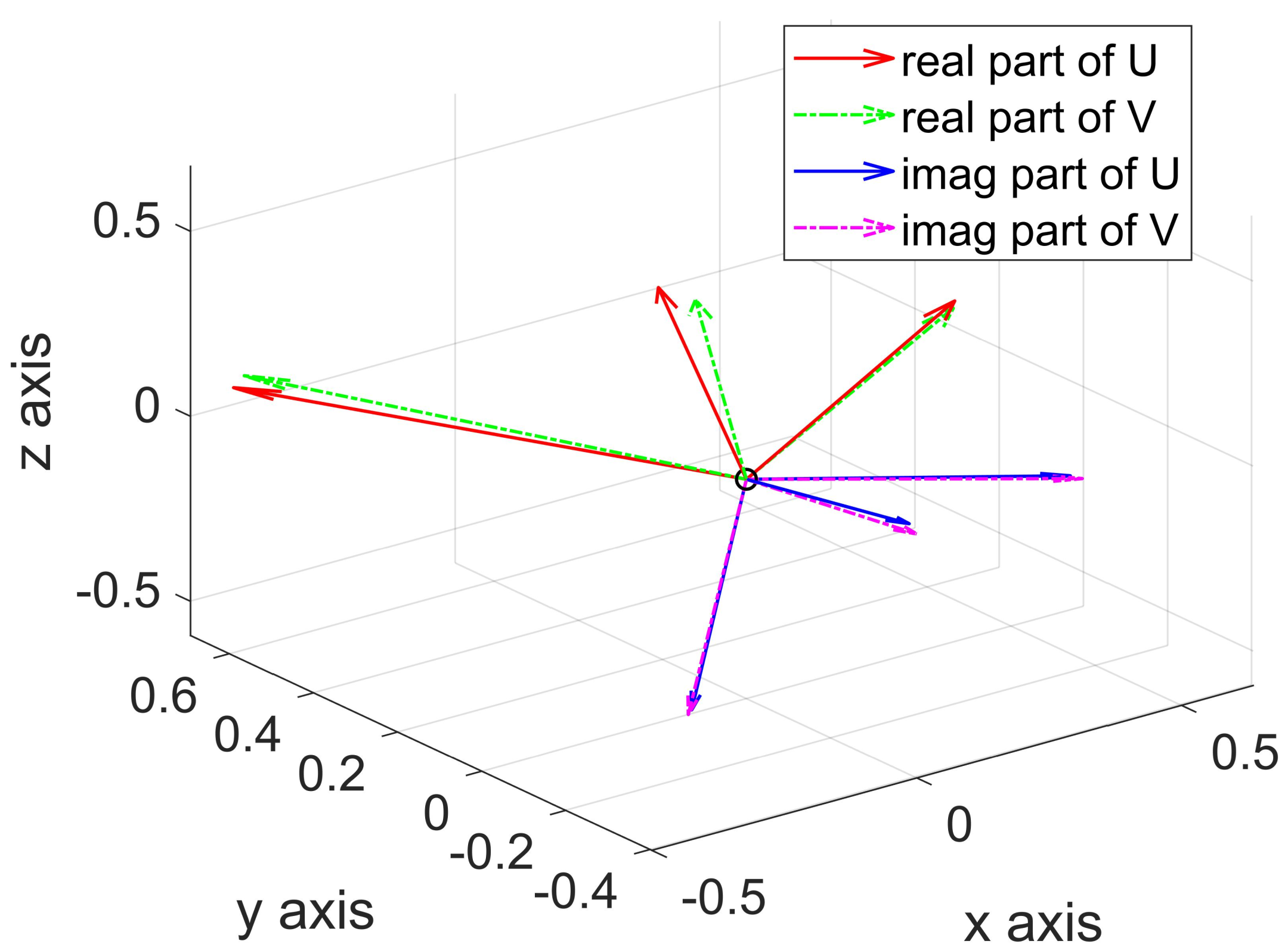
Figure 2 presents the relationship between the eigenvectors. The figure illustrates that the eigenvectors corresponding to the similar eigenvalue are close. To avoid the eigendecompositions, we use the relation in power methods to compute the eigenvectors [43].
Assuming the matrix B C n × n has n linearly independent eigenvectors v i , i = 1 , 2 , n and eigenvalues λ i , i = 1 , 2 , n
B v i = λ i v i , λ 1 λ 2 λ n
The power method starts from a vector b 0 , which can be a random vector or an approximation of the dominant eigenvector of the matrix. The method can be written as follows [43]
b k + 1 = B b k
The vector b k is multiplyed by B at each iteration. These linearly independent eigenvectors form a basis of n-dimensional space. Therefore, b 0 can be written as a linear combination of the n eigenvectors
b 0 = i = 1 n α i v i
Thus b 1 = B b 0 = i = 1 n α i λ i v i . Generally
b k + 1 = B b k = i = 1 n α i λ i k v i = λ 1 k i = 1 n α i λ i λ 1 k v i
For sufficiently large k,
λ i λ 1 k 0
So, we have
b k + 1 λ 1 k α 1 v 1
The eigenvalue and eigenvector can be computed from
λ 1 b k + 1 1 / b k 1 , v 1 b k + 1
Taking the arithmetic overflow into consideration, the normalization is usually performed in actural calculation. Thus, the iteration can be writen as
b k + 1 = B b k B b k
The power method converges to the eigenvector corresponding to the eigenvalue with the largest amplitude. The least eigenvalue in amplitude can be obtained by the inverse power method.
In our problem, the eigenvalue must be real because T , A k are Hermitian matrices. The boundary points on the BCR correspond to the largest and smallest eigenvalues. However, the power methods can only obtain the largest and least eigenvalues in amplitude. As the eigenvalues are sorted differently, the eigenvectors are not always identical. Figure 3 illustrates two cases in eigenvalue sorting. In the first case, the eigendecomposition and the power methods get the same eigenpairs. However, in Case 2, they are different. To solve this problem, we use a theorem as follows
Theorem 1
([44] ). Let p ( t ) be a given polynomial of degree k. If  ( λ , x ) is an eigenvalue–eigenvector pair of B C n × n , then ( p ( λ ) , x ) is an eigenvalue–eigenvector pair of p ( B ) .
Therefore, a proper identity matrix can be added to change the eigenvalues while the eigenvectors remain unchanged
B ˜ = B + θ I
Note that the coefficient θ is of importance. On the one hand, θ should ensure that all the eigenvalues of B ˜ are positive. On the other hand, the identity matrix should not change the relationship between A k and A k + 1 . For example, if  θ is large enough, the matrix B ˜ becomes a diagonally dominant matrix leading to the failure of the phase rotations algorithm. The spectral radius of a square matrix is the largest absolute value of its eigenvalues [44]
ρ ( B ) = max | λ B |
ρ ( B ) precisely satisfies the requirement of θ . However, computing the spectral radius is also an eigendecomposition work. The spectral radius is the lower bound of any norm of matrix [44], so we use the 2-norm.
After a series of transformations, the orders of eigenvalues are consistent. To keep notation light, we rewrite the problem
B 0 = T 1 ( Ω + Ω H ) B k = T 1 ( e j ϕ k Ω + e j ϕ k Ω H )
Since the eigenvectors of B and B ˜ are close, the eigenvectors of B k are set as the initial vector of power methods in solving eigenvectors of B k + 1 . The power methods can reach high accuracy after several iterations. The IEBCR is summarized in Algorithm 1.
Algorithm 1. IEBCR.
1:
Input: The polarimetric interferometric matrix Ω , the coherence matrix T, the phase step ϕ
2:
Output: The boundary coherence vector γ C 2 n
   % main precedure: %
3:
Eigendecomposition of B 0 = T 1 ( Ω + Ω H )
4:
Sort the eigenvalues, λ 1 > λ 2 > λ 3 , with eigenvectors v 1 , v 2 , v 3 . Calculate γ 1 , γ 2 according to Equation (3) using v 1 , v 2 .
5:
Calculate the spectral norm of B 0 , θ = B 0 2 .
6:
   % main loop: %
7:
for   k = 2 : n   do
8:
       B k = T 1 ( e j k ϕ Ω + e j k ϕ Ω H )
9:
       B k ˜ = B k + θ I
10:
       v 1 = Power Method ( v 1 , B k ˜ )
11:
       v 3 = Inverse Power Method ( v 3 , B k ˜ )
12:
       γ 2 k 1 = v 1 H Ω v 1 / v 1 H T v 1
13:
       γ 2 k = v 3 H Ω v 3 / v 3 H T v 3
14:
       k = k + 1
15:
end loop
In the algorithm, the 2-norm is not calculated in each iteration. First, calculating the 2-norm in each iteration is time-consuming. More importantly, using the norm of B 0 is feasible in actual calculations.

3.2. ILUT

In the final stage of TSIA, the exhaustive search strategy to get the optimal parameters in the defined step sizes brings high computational complexity. To explore the property of loss function in Equation (10), we define the RVoG function as follows
f = p 1 p 2 e p 2 h v 1 e p 1 h v 1 2
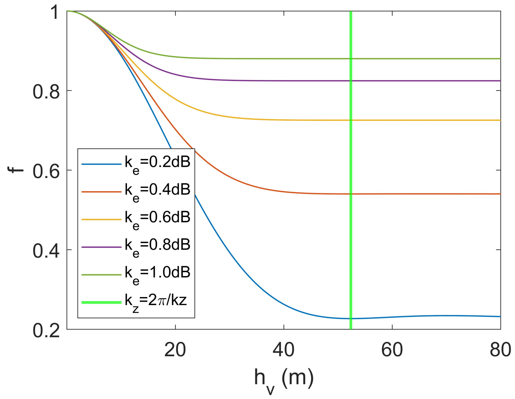
From the function plots in Figure 4, the function seems to have the following characteristics.
1.
For a fixed k e , the function converges to a value as the tree height increases. Moreover, the value increases with the increase of k e .
2.
In the direction of h v , the function is monotonically decreasing in a specific interval.
3.
In the direction of k e , the function is monotonically increasing.
In the following text, we will attempt to prove these properties from analytic and numerical points of view.

3.2.1. Convergence Properties

The linear relationship between p 1 and k e does not influence the characteristics of the function. For convenience, we use p 1 to represent k e in proving text. To illustrate the convergence, we simplify f using Euler’s formula as follows
f = p 1 p 1 + j k z 2 e p 1 h v e j k z h v 1 e p 1 h v 1 2 = p 1 2 p 1 2 + k z 2 1 + 2 e p 1 h v e p 1 h v 1 2 1 cos k z h v
The first part is independent of h v . When h v is sufficiently large, we have
= lim h v p 1 2 p 1 2 + k z 2 1 + 2 e p 1 h v e p 1 h v 1 2 1 cos k z h v = p 1 2 p 1 2 + k z 2
The above expression is monotonically increasing with p 1 . Moreover, as  p 1 operates on the exponential term, the curve converges faster when p 1 is larger.
We next prove that the minimum value of the function is the convergence value.
The second part of f has a concise geometric interpretation as shown in Figure 5. According to the triangle inequality, the difference between any two sides of a triangle must less than the length of the third side. So, the length of the orange vector is larger than that of the green vector. So, we have
e p 1 h v + j k z h v 1 e p 1 h v 1 > 1 f > p 1 2 p 1 2 + k z 2
Moreover,
f 2 n π k z = p 1 2 p 1 2 + k z 2 , n = 1 , 2 ,
where 2 n π 2 n π k z k z is the ambiguity height. It demonstrates that the inversion capability of the RVoG model is [ 0 , 2 π / k z ] . Therefore, we infer that the monotonic interval in the h v direction is [ 0 , 2 π / k z ] . Next, we will prove the monotoncity of f in both directions.

3.2.2. Monotoncity

The partial derivative of the RVoG function with respect to h v is
f h v = p 1 2 e p 1 h v p 1 2 + k z 2 e p 1 h v 1 3 k z sin k z h v e p 1 h v 1 p 1 1 cos k z h v e p 1 h v + 1
Apparently, the ambiguity heights are the stationary points that satisfy the following equation
f h v 2 n π k z = 0 , n = 1 , 2 ,
It is challenging to determine whether there are other stationary points because of the exponential and trigonometric terms. For a fixed h v , the derivative changes with p 1 and k z , and we can judge its sign according to the numerical computation. However, we can not exhaust all h v in the range of [ 0 , 2 π / k z ] to prove the monotoncity. To achieve this goal, we carry out the following transformation
t = p 1 / k z , x = k z h v , 0 < x < 2 π
With the transformation, the derivative function has two variables left and can be written as
f x t 2 t 2 + 1 e t x e t x 1 3 e t x 1 sin x t 1 cos x e t x + 1
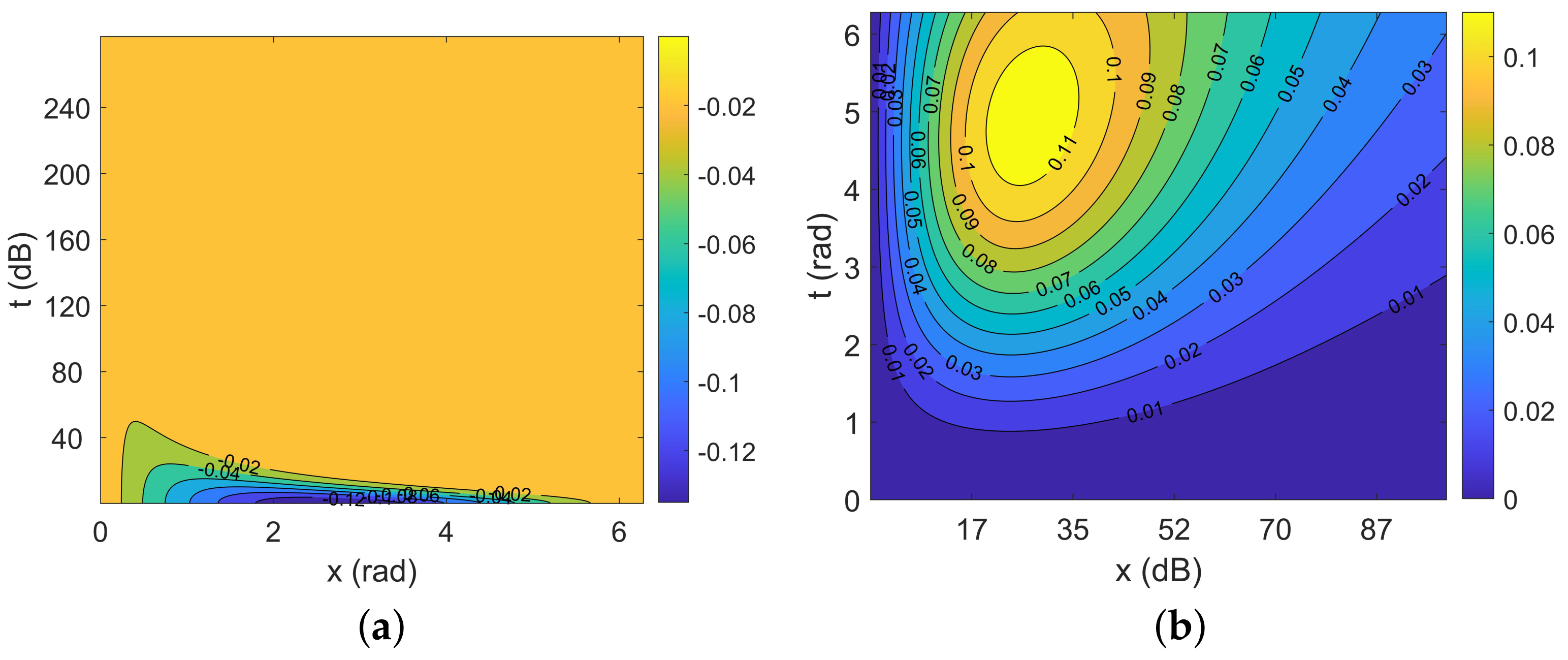
Figure 6a provides the contour map of the derivative function. The derivative function is always negative, which means the function f is monotonically decreasing in [ 0 , 2 π / k z ] .
The partial derivative of the RVoG function with respect to p 1 can be written as follows
f p 1 = p 1 p 1 2 + k z 2 2 k z 2 p 1 2 + k z 2 + 2 ( 1 cos ( k z h v ) ) e p 1 h v e p 1 h v 1 2 · 2 k z 2 p 1 2 + k z 2 p 1 h v e p 1 h v + 1 e p 1 h v 1
Similarly, in order to explain the sign of the derivative more conveniently, we apply the following transformation
x = p 1 h v , t = k z h v , 0 < t < 2 π
So, the derivative becomes
f x 2 x t 2 x 2 + t 2 2 1 + 2 e x e x 1 2 1 cos t 2 1 cos t x 2 x 2 + t 2 e x e x + 1 e x 1 3
Figure 6b presents the contour of the derivative. The positive derivative demonstrates that f is monotonically increasing in the p 1 direction.

3.2.3. ILUT

The RVoG function and loss function have different geometric interpretations despite similar forms. In the 2-D complex plane, the loss function denotes the Euclidean distance between the calculated coherence and the observed coherence. The RVoG function denotes the Euclidean distance between the thetical coherence and the origin.
Figure 7 shows the geometrical representation and the contour of the loss function. The black rectangles indicate the neighborhood near the optimal solution. In the complex space, the neighborhood has a rather small distance that corresponds to the blue band areas in the contour map. After analysis, the optimization problem does not exhibit particularly irregular properties. Therefore, as long as the neighborhood of the optimal solution can be found in the initial search, a new grid can be established locally to get a better solution. Figure 7 inspires us that the iterative LUT (ILUT) can be established in the inversion process. Specifically, a coarse grid is first established to search the neighborhood near the optimal solution, then a series of refined grids can be established in the neighborhood for the optimal solution. Algorithm 2 provides the details of ILUT.
Moreover, the loss function is more sensitive in the direction of h v than that of k e . Therefore, in the contour map, blue band areas appear near the optimal solution in the direction of k e . Thus, a fixed extinction coefficient, assuming 0.4 dB/m, can still achieve reasonable inversion results despite the loss of accuracy. Some scholars have tried this during the inversion process [8,37], and our analysis verifies the rationality of this approach.
Algorithm 2. ILUT.
1:
Input: The candidate of volume coherence γ v ˜ , the range of k e : k e m a x , k e m i n , the range of h v : h v m a x , h v m i n , the precision Δ k e and Δ h v .
2:
Output: The inversion height h v ˜ , k e ˜ and the loss function value l o s s
   % main precedure: %
3:
The initial step Δ h v i , Δ k e i , the ratio of step m
4:
   % main loop: LUT inversion: h b e s t , k e b e s t , l o s s %
5:
while Δ h v i > Δ h v
6:
    h v m i n = h b e s t Δ h v i , h v m a x = h b e s t + Δ h v i
7:
    k e m i n = k b e s t Δ k e i , k e m a x = k b e s t + Δ k e i
8:
    Δ h v i = Δ h v i / m
9:
    Δ k e i = Δ k e i / m
10:
end loop

4. Results

4.1. Data Description

This paper uses European Space Agency (ESA) BioSAR 2008 data [45] to verify the effectiveness of the proposed algorithms. The data were acquired by the German Aerospace Center (DLR) E-SAR system in Northern Sweden. The test site is mainly confined within the Krycklan River catchment (KCS). The KCS is 6790 ha in area and comprises a mosaic of instrumented and well-studied forests, agriculture, wetlands, and lakes, all drained and connected by a network of streams and rivers [46]. Mixed coniferous forest is the dominating forest type, primarily between 0–35 m in height. The data contains airborne SAR data and the LiDAR H100 data. The SAR images are Single Look Complex (SLC) format with four polarization channels: HH, HV, VH and VV. The SAR data were acquired in two different flight directions with various spatial baselines. First flight direction is 313 with a southwest radar look direction. The other flight direction is 133 with the northeast radar look direction. Table 1 provides some details of the PolInSAR data. In this paper, the researched data is 6 m baseline at L-band and 24 m baseline at P-band. The reference height for validation is the LiDAR H100, which is defined as the mean height of the 100 highest trees per hectare [47]. Previous works have well demonstrated that the LiDAR H100 can provide precise measurement for forest canopy height [6,47].
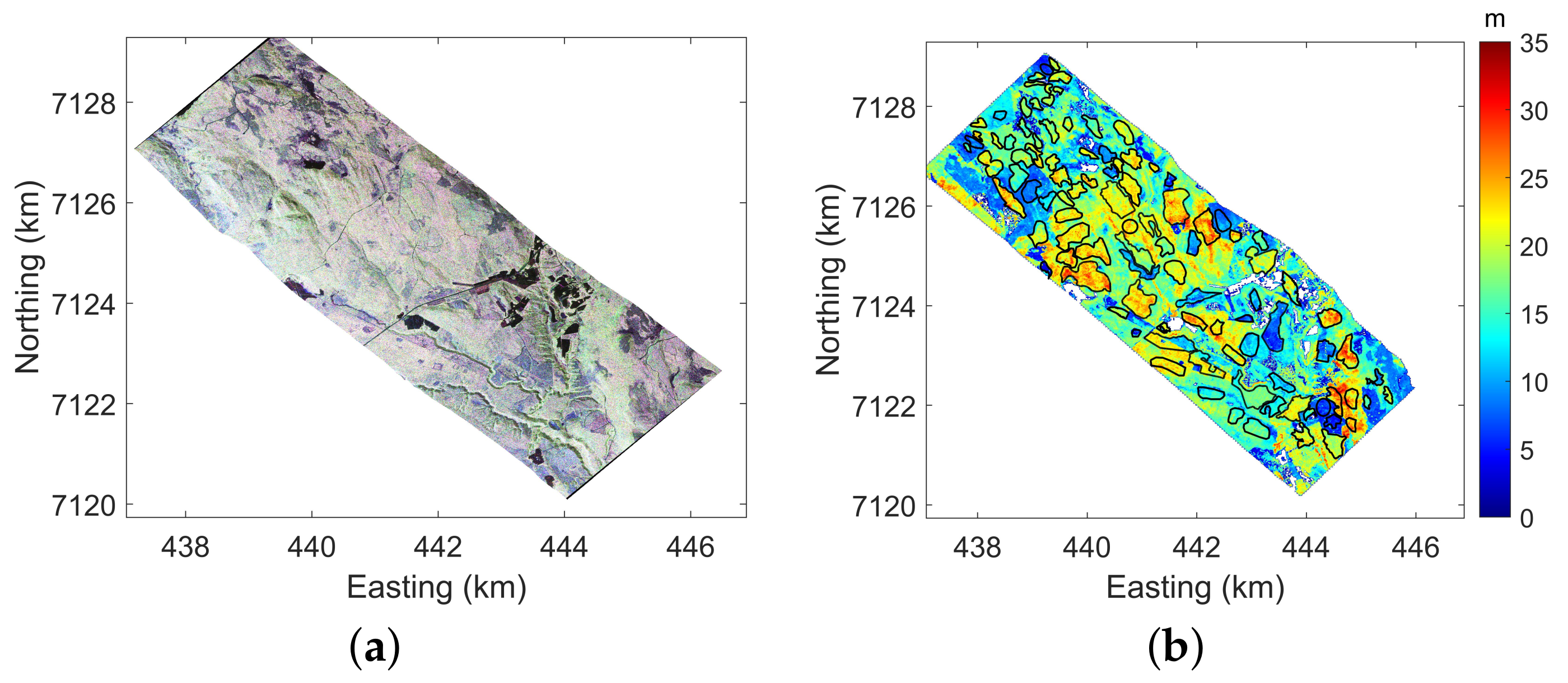
Figure 8a shows the Pauli-basis polarimetric composite image. Figure 8b provides the LiDAR H100 forest height map. It is worth noting that the resolution of the LiDAR map and geocoded SAR images is 10 m × 10 m, 1 m × 1 m, respectively.

4.2. Evaluation Indicator

The valuation indicators used to evaluate the results are: mean error m, root mean square error (RMSE) r, correlation coefficient ρ , and accuracy α . The indicators are defined as follows
m = 1 K k = 1 K h k ˜ h k
r = 1 K k = 1 K ( h k ˜ h k ) 2
ρ = Cov ( h ˜ , h ) Var ( h ˜ ) Var ( h )
α = 1 K k = 1 K I | h k ˜ h k | < σ
where Cov is the covariance function and Var is the variance function. I | h k ˜ h k | < σ is the indicative function defined as flows
I | h k ˜ h k | < σ = 1 , if | h k ˜ h k | < σ 0 , otherwise .

4.3. Forest Height Inversion

Part 1 in Figure 1 illustrates the processing flowchart. The preprocessing includes coregistration, flat-ground phase removal, geocoding, and coherence estimation. The coregistration has been performed by DLR [45]. The flat-ground phase removal can be completed according to the flat-ground phase files. After the flat-ground phase removal, the coregistered image can be converted into geocoded geometry using conversion matrices, which are included in the master products. The coherences are calculated using a boxcar filtering, with a sliding window size of 7 × 7. The boxcar filtering can reduce the speckle noise of SAR images and the output pixel value is an average of pixels in the sliding window.
Since the resolution of the LiDAR data is different from that of the PolInSAR forest map, an interpolation is processed on LiDAR data to better compare the inversion results. The bicubic interpolation [48] is performed to generate a more reasonable interpolation result. Specifically, the output pixel value is a weighted average of pixels in the nearest 4 × 4 neighborhood. If there is no particular illustration in the following text, the LiDAR H100 has been interpolated.
To facilitate the further analysis of the two iterative algorithms, four sets of comparative experiments are implemented at both bands, respectively. Concretely, the experimental configurations are carried out, i.e., (a) TSIA + EBCR + LUT, (b) TSIA + IEBCR + ILUT, (c) TSIA + EBCR + ILUT, and (d) TSIA + IEBCR + LUT. Note that all the configurations follow the same processing flow shown in Figure 1. The difference between IEBCR and EBCR is whether using the relationship between the eigenvectors of adjacent points on the boundary. Moreover, the power methods are used to obtain the eigenvector in the extraction of BCR, and the termination condition of the power methods is identical. At the same time, the step size of height and extinction in the ILUT and LUT is the same.

4.4. Forest Height Validation

As shown in Figure 8b, 105 polygons over the entire test site are selected from the original LiDAR H100 to provide validation for the estimated height. To reduce the influence of topographic variation, each individual polygon is selected only from the homogenous areas. For better validation, all the estimated heights were transformed from slant range geometry to the UTM Zone 34 coordinate.

4.4.1. P-Band

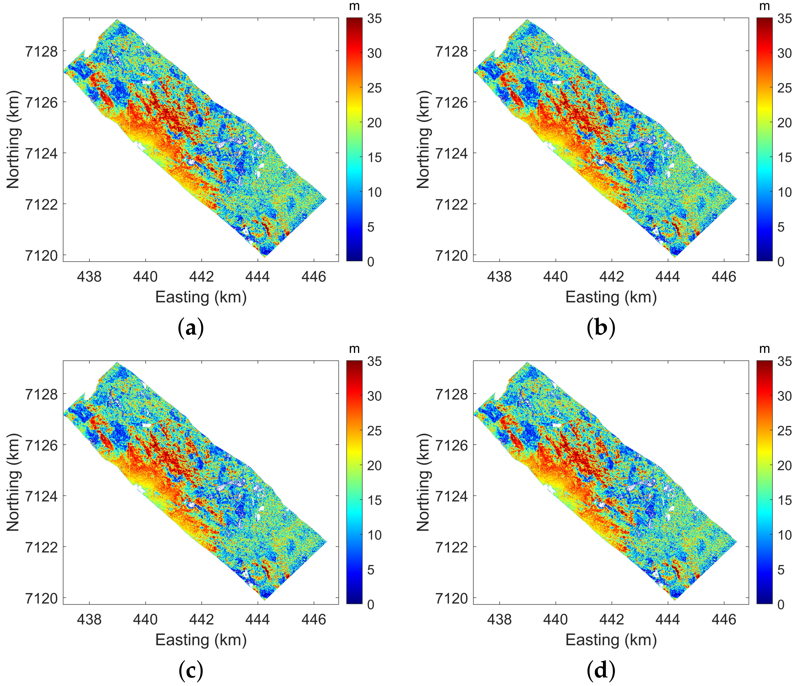
Figure 9 provides the inversion height maps from P-band data. All the color ramps range from 0 to 35 m for convenient comparisons with the LiDAR H100. The influence of IEBCR and ILUT on the inversion accuracy can be obtained from the following comparisons. Concretely, the difference between IEBCR and EBCR can be obtained from Figure 9a,d. The difference between ILUT and LUT can be acquired from Figure 9a,c. The total influence of IEBCR and ILUT can be seen from Figure 9a,b. The estimated heights of the four sets of experiments are almost the same in terms of visual effects. It demonstrates that the proposed iterative algorithms almost have no deterioration on the inversion results. To further evaluate the estimated heights, the mean value of each polygon is calculated from the LIDAR H100 and the Pol-InSAR estimated height separately. The correlation plots and the evaluation indicators in 105 polygons are shown in Figure 10. As shown in Figure 10a, the inversion heights from TSIA + EBCR + LUT reach the mean error of −2.08 m, the RMSE of 4.92 m, the correlation coefficient of 0.58, and the accuracy of 61.54%. Figure 10b–d show the similar indicators.

4.4.2. L-Band

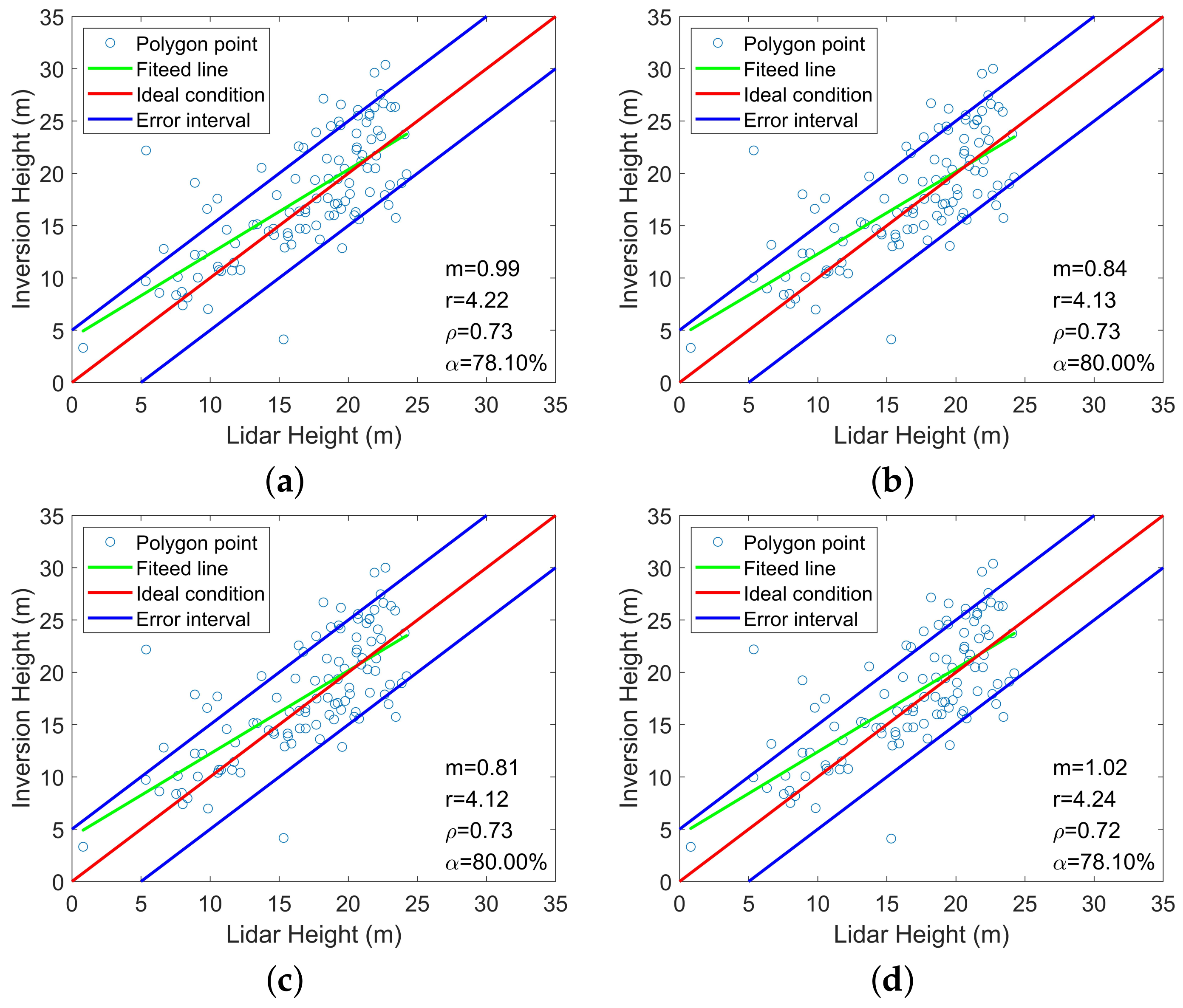
Figure 11 shows the inversion height maps from L-band data and Figure 12 presents the comparisons and the evaluation indicators in polygons. The similar inversion results in Figure 11a–d indicates that the iterative methods are also valid at L-band. As shown in Figure 12a, the inversion heights from TSIA + EBCR + LUT reach the mean error of 0.99 m, the RMSE of 4.22 m, the correlation coefficient of 0.73, and the accuracy of 78.10%. Figure 12b–d show the similar indicators.

5. Discussion

5.1. Quality of Forest Height Estimation

For both bands, the indicators of the estimated height maps from different experimental configurations are quite similar. The L-band inverted heights correlated better with LiDAR H100 than that of the P-band. As shown in Figure 10 and Figure 12, the height estimates at P-band suffer a more serious underestimation than L-band. The main reason may be interpreted from the stronger penetration from P-band. First, the ground contribution in all polarimetric channels makes the estimation of the volume-only coherence a challenge. Although γ h is regarded as the best candidate for volume-only coherence, the GVR still cannot be neglected. Second, the strong penetration introduces more uncertainty in the sorting of GVR at different polarization channels, which makes Equation (8) fail, resulting in the wrong choice of γ h and ground phase.

5.2. Analysis of IEBCR

5.2.1. Analysis of the Accuracy

To better evaluate the accuracy of the IEBCR, we compare the inversion results from different experiment configurations. Specifically, we analyzed the results from TSIA + IEBCR + ILUT and TSIA + EBCR + ILUT. Figure 13 presents their absolute difference of estimated heights. As shown in Figure 13c, most areas show a difference smaller than 1 m at both bands. In the valid areas, the difference is equal to 0 in 63% of the pixels at P-band and 75% at L-band. The comparisons illustrate that the IEBCR achieves almost the same inversion results.

5.2.2. Analysis of Efficiency

The relationship of eigenvectors between adjacent boundary points is changing with the phase spacing. Specifically, the smaller the phase spacing, the closer the eigenvectors. Furthermore, the closer the eigenvectors, the faster convergence. Therefore, the efficiency should be changed with the number of points on BCR.
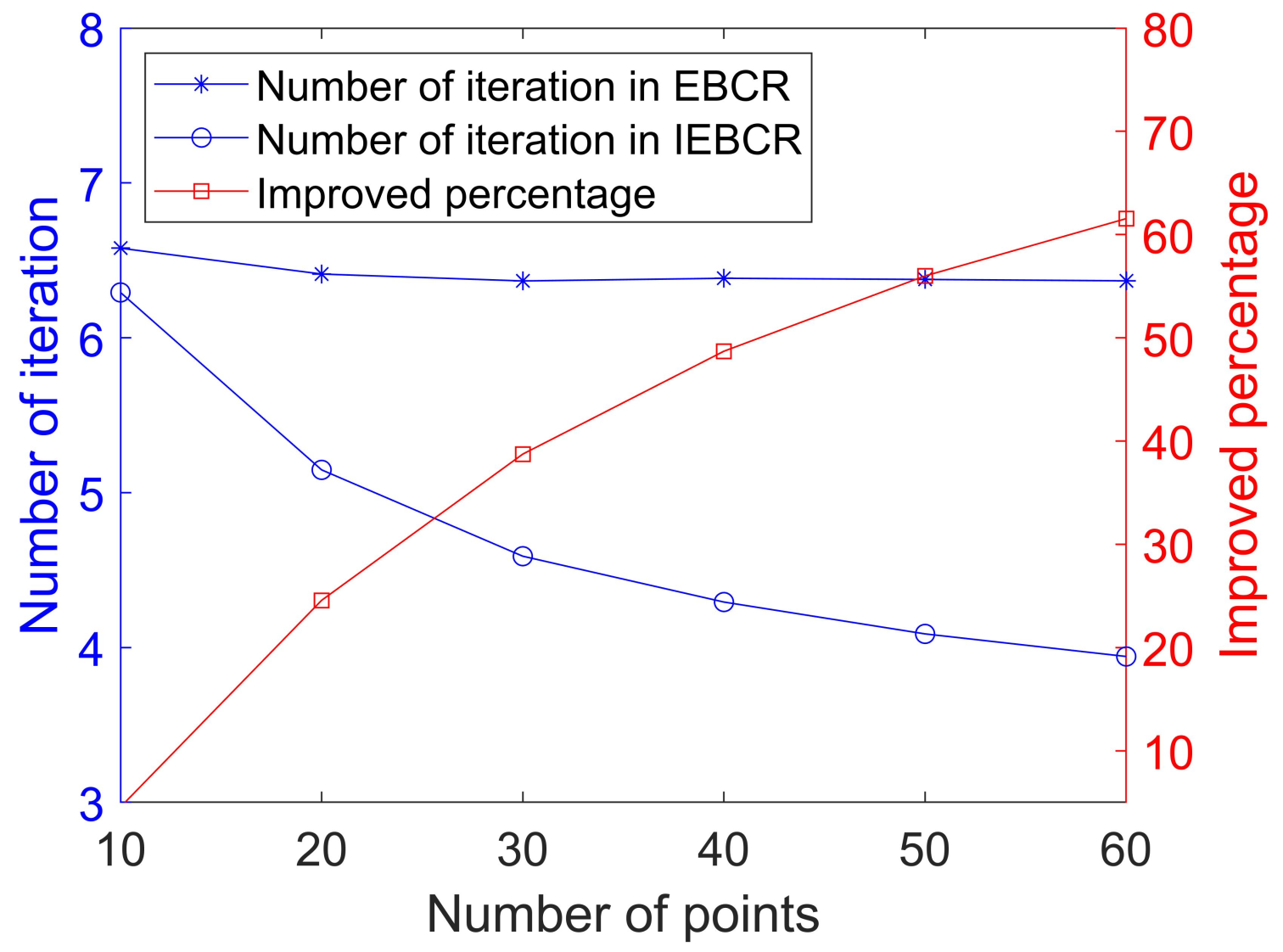
To evaluate the efficiency, we performed the Monte Carlo experiments in ERCR and IEBCR methods. In the tested area, the power methods are applied to calculate the BCR for each pixel. We set N in the range of [ 10 , 60 ] with a spacing of 10. For each N, the BCR of 1000 pixels is extracted. Figure 14 depicts the average number of iterations in ERCR and IEBCR and the improved curve on efficiency. As shown in the figure, the number of iterations in ERCR is almost not varied with N. However, the number of iterations in IEBCR is decreased with the increase of N. Thus, the improved efficiency rise with the increase of N. It is consistent with our above analysis. Taking N = 30 in practice provides a good trade-off between accuracy and efficiency.

5.3. Analysis of ILUT

5.3.1. Analysis of the Accuracy

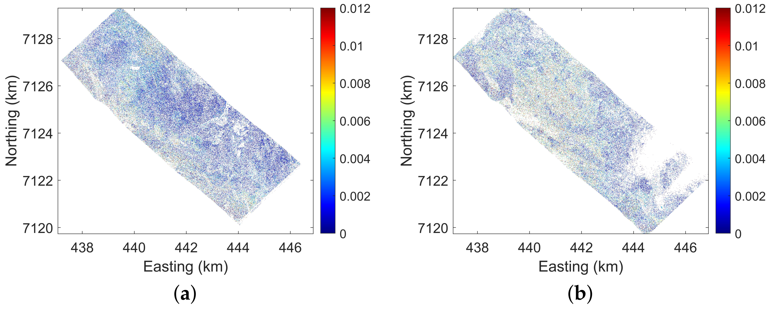
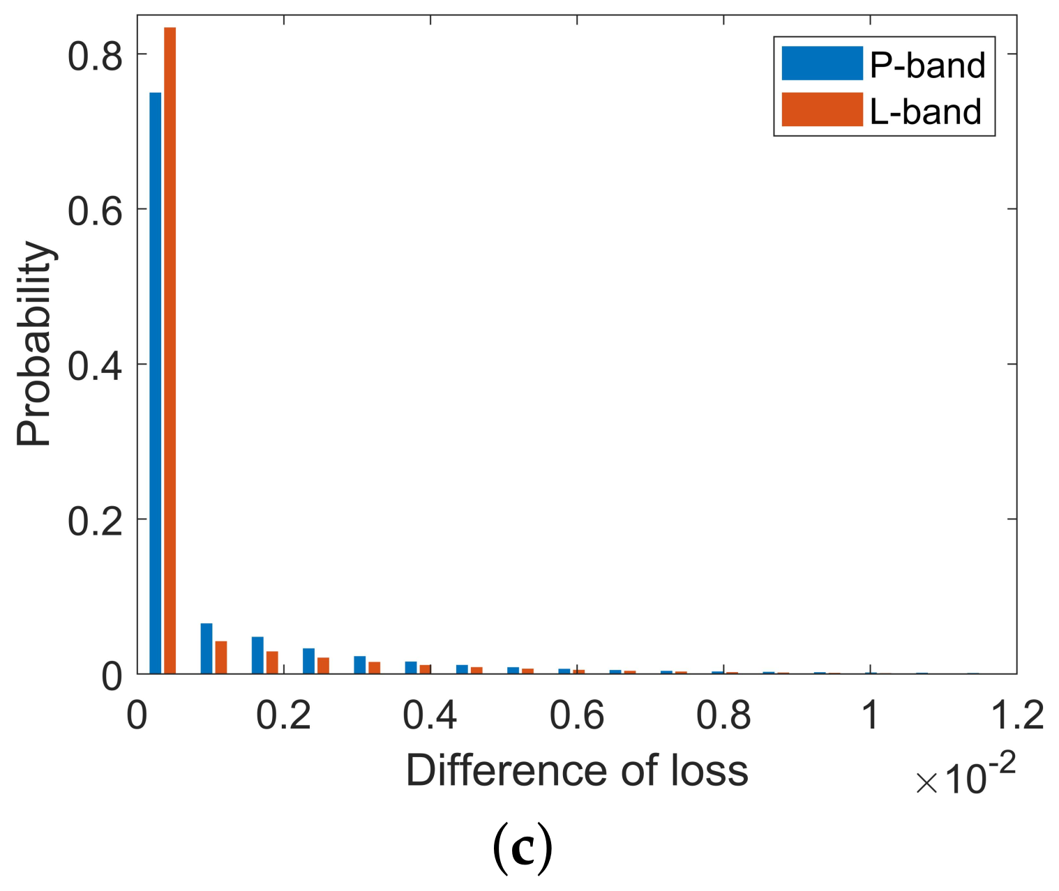
To better evaluate the accuracy of the ILUT, we compare the inversion results from different experiment configurations. Concretely, we analyzed the results from TSIA + IEBCR + ILUT and TSIA + IEBCR + LUT. Figure 15 illustrates the absolute difference of loss between them. The difference is less than 0.01 in more than 99% of the area at both bands. In the numerical calculation, the difference is negligible. The main reason for the error is the height-extinction ambiguity in the interpretation of the interferometric coherence. High forest with a high extinction coefficient generates the same loss function as a low forest with a lower extinction coefficient [28,29].

5.3.2. Analysis of the Efficiency

Assuming that the range of h v is ( 0 , h v m ) , the range of k e is ( 0 , k e m ) , and the precisions are Δ h v , Δ k e , respectively. The number of the grid points in LUT and ILUT is respectively
N L U T = h v m Δ h v · k e m Δ k e
N I L U T = h v m Δ h v 1 · k e m Δ k e 1 + ( q 1 ) · ( 2 m + 1 ) 2
where Δ h v 1 and Δ k e 1 is the precision in the first search grid of ILUT, q represents the total number of iterations, ( 2 m + 1 ) 2 is the number of the grid points in the second and subsequent iterations.
In the inversion process, the consumed time to calculate the coherence based on the model and to search the minima in the grid are linearly dependent on the number of grid points. Therefore, the ratio of the computational complexity can be written approximately as
β = N L U T N I L U T = h v Δ h v · k e Δ k e h v Δ h v 1 · k e Δ k e 1 + ( q 1 ) · ( 2 m + 1 ) 2
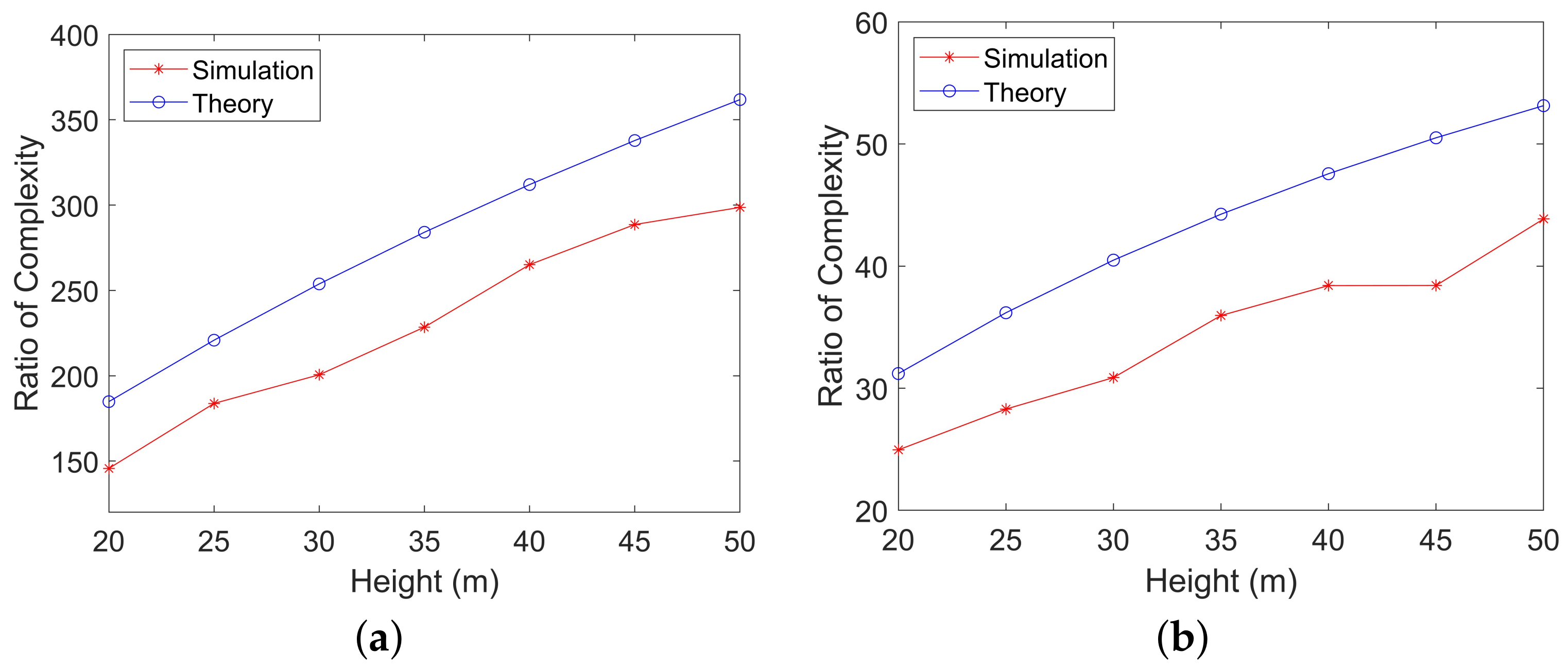
We carry out two sets of experiments to verify the above theoretical analysis. In the first experimental configuration, we set Δ h v = 0.01 m, Δ k e = 0.01 dB/m, Δ h v 1 = 1 m, Δ k e 1 = 0.1 dB/m, q = 3 and k e m = 1 dB/m. In the second case, we set Δ h v = 0.1 m, Δ k e = 0.01 dB/m, Δ h v 1 = 1 m, Δ k e 1 = 0.1 dB/m, q = 2 , and k e m = 1 dB/m. With these fixed parameters, the ratio of computational complexity relies on the h v m . We set h v m in the range of 20–50 m with a spacing of 5 m. For each value of h v m , 1000 observed coherences are calculated by Equation (6), where the height and extinction are randomly sampled in their respective ranges. Then, we apply LUT and ILUT respectively and record the ratio of consumed time.
Figure 16 provides the theoretical and simulated complexity ratio. Although there are differences between them, the trends of the curves demonstrate a good correspondence. In programming, the vectorized and parallel strategies may affect the actual ratio of consumed time, but the theoretical analysis ensures that the ILUT significantly improves the computational efficiency.

5.4. Limitations of the Proposed Methods

From the results discussed above, even if IEBCR improves the efficiency by around 40% ( N = 30 ), the efficiency still needs to be further improved in practice for large-scale forest height estimation. The main reason is that the analytical form in Equation (13) is not derived. The relationship of the eigenvectors is complex and needs further study.

6. Conclusions

This study set out to enhance the computational efficiency of EBCR and LUT in the TSIA. The IEBCR and ILUT iterative methods are introduced and analyzed. Given many eigendecompositions in the EBCR, we analyzed the relationship of eigenvectors of the adjacent points on the BCR. The analysis manifests the eigenvectors are close in the Euclidean space. Therefore, we proposed the IEBCR utilizing the relationship of eigenvectors. In the final stage, we define the RVoG function and prove its monotonicity and convergence from the analytical and numerical points of view. The proof indicates that the loss function in the LUT does not exhibit extreme irregular properties. Therefore, we propose the iterative LUT (ILUT) for the inversion stage.
The experiments are carried out to verify the effectiveness of the proposed algorithms based on the BioSAR 2008 PolInSAR data at P- and L-bands. The results demonstrate that
1.
The two iterative methods are effective at P- and L-bands in single-baseline forest height inversion.
2.
The iterative methods can significantly improve the computational efficiency without compromising on the accuracy and are applicable to various algorithms for retrieval of forest vertical structure based on the RVoG model.

Author Contributions

Conceptualization, Z.H.; methodology, Z.H.; software, Z.H.; validation, Z.H. and X.L.; formal analysis, Z.H.; investigation, Z.H.,Y.Y., X.L. and H.C.; resources, Z.H., Y.Y., H.C. and X.L.; data curation, Z.H. and H.C.; writing—original draft preparation, Z.H.; writing—review and editing, Z.H. and X.L.; visualization, Z.H., Y.Y., X.L. and H.C.; supervision, Z.H., Y.Y., H.C. and X.L.; project administration, X.L., Y.Y. and H.C.; funding acquisition, X.L. and Y.Y. All authors have read and agreed to the published version of the manuscript.

Funding

This work was supported in part by the National Natural Science Foundation of China under Grant 41801356 and in part by the LuTan-1 L-Band Spaceborne Bistatic SAR data processing program under Grant E0H2080702.

Institutional Review Board Statement

Not applicable.

Informed Consent Statement

Not applicable.

Data Availability Statement

The BioSAR 2008 campaign data is available on https://earth.esa.int/eogateway/campaigns/biosar-2 (accessed on 16 May 2022) via FTP upon submission of a data access request.

Acknowledgments

The authors would like to thank the European Space Agency(ESA) for providing the BioSAR 2008 dataset (ESA EO Project Campaign ID 69499).

Conflicts of Interest

The authors declare no conflict of interest.

Abbreviations

The following abbreviations are used in this manuscript:
RVoGRandom Volume over Ground
TSIAthree-stage inversion algorithm
LiDARLight Detection And Ranging
PolInSARPolarimetric Interferometric Synthetic Aperture Radar
GVRground-to-volume amplitude ratio
NGVRnull ground-to-volume amplitude ratio
RMoGRandom-Motion-over-Ground
VTDvolume temporal decorrelation
BCRboundary of the coherence region
EBCRextraction of the boundary of the coherence region
IEBCRiterative extraction of the boundary of the coherence region
LUTlook-up table
ILUTiterative look-up table
RMSEroot mean square error

References

  1. Toan, T.L.; Villard, L.; Lasne, Y.; Mermoz, S.; Koleck, T. Assessment of tropical forest biomass: A challenging objective for the biomass mission. In Proceedings of the 2012 IEEE International Geoscience and Remote Sensing Symposium, Munich, Germany, 22–27 July 2012; pp. 7581–7584. [Google Scholar] [CrossRef]
  2. Bergen, K.M.; Goetz, S.J.; Dubayah, R.O.; Henebry, G.M.; Hunsaker, C.T.; Imhoff, M.L.; Nelson, R.F.; Parker, G.G.; Radeloff, V.C. Remote sensing of vegetation 3-D structure for biodiversity and habitat: Review and implications for lidar and radar spaceborne missions. J. Geophys. Res. Biogeosci. 2009, 114, G00E06. [Google Scholar] [CrossRef] [Green Version]
  3. Le Toan, T.; Quegan, S.; Davidson, M.W.J.; Balzter, H.; Paillou, P.; Papathanassiou, K.; Plummer, S.; Rocca, F.; Saatchi, S.; Shugart, H. The BIOMASS mission: Mapping global forest biomass to better understand the terrestrial carbon cycle. Remote Sens. Environ. 2011, 115, 2850–2860. [Google Scholar] [CrossRef] [Green Version]
  4. Agata, H.; Aneta, L.; Dariusz, Z.; Krzysztof, S.; Marek, L.; Christiane, S.; Carsten, P. Forest Aboveground Biomass Estimation Using a Combination of Sentinel-1 and Sentinel-2 Data. In Proceedings of the IGARSS 2018—2018 IEEE International Geoscience and Remote Sensing Symposium, Valencia, Spain, 22–27 July 2018; pp. 9026–9029. [Google Scholar] [CrossRef]
  5. Lefsky, M.A.; Cohen, W.B.; Parker, G.G.; Harding, D.J. Lidar Remote Sensing for Ecosystem Studies: Lidar, an emerging remote sensing technology that directly measures the three-dimensional distribution of plant canopies, can accurately estimate vegetation structural attributes and should be of particular interest to forest, landscape, and global ecologists. BioScience 2002, 52, 19–30. [Google Scholar] [CrossRef]
  6. Pourshamsi, M.; Xia, J.; Yokoya, N.; Garcia, M.; Lavalle, M.; Pottier, E.; Balzter, H. Tropical forest canopy height estimation from combined polarimetric SAR and LiDAR using machine-learning. ISPRS J. Photogramm. Remote Sens. 2021, 172, 79–94. [Google Scholar] [CrossRef]
  7. Papathanassiou, K.P.; Cloude, S.R. Single-baseline polarimetric SAR interferometry. IEEE Trans. Geosci. Remote Sens. 2001, 39, 2352–2363. [Google Scholar] [CrossRef] [Green Version]
  8. Garestier, F.; Dubois-Fernandez, P.C.; Champion, I. Forest height inversion using high-resolution P-band Pol-InSAR data. IEEE Trans. Geosci. Remote Sens. 2008, 46, 3544–3559. [Google Scholar] [CrossRef]
  9. Soja, M.J.; Persson, H.; Ulander, L.M.H. Estimation of forest height and canopy density from a single InSAR correlation coefficient. IEEE Geosci. Remote Sens. Lett. 2014, 12, 646–650. [Google Scholar] [CrossRef] [Green Version]
  10. Kugler, F.; Koudogbo, F.; Gutjahr, K.; Papathanassiou, K. Frequency effects in Pol-InSAR forest height estimation. In Proceedings of the European Conference on Synthetic Aperture Radar (EUSAR), Dresden, Germany, 16–18 May 2006; pp. 1–4. [Google Scholar]
  11. Zhao, L.; Chen, E.; Li, Z.; Zhang, W.; Fan, Y. A New Approach for Forest Height Inversion Using X-Band Single-Pass InSAR Coherence Data. IEEE Trans. Geosci. Remote Sens. 2021, 60, 5206018. [Google Scholar] [CrossRef]
  12. Sun, X.; Wang, B.; Xiang, M.; Zhou, L.; Jiang, S. Forest Height Estimation Based on P-Band Pol-InSAR Modeling and Multi-Baseline Inversion. Remote Sens. 2020, 12, 1319. [Google Scholar] [CrossRef] [Green Version]
  13. Soja, M.J.; Persson, H.J.; Ulander, L.M.H. Modeling and Detection of Deforestation and Forest Growth in Multitemporal TanDEM-X Data. IEEE J. Sel. Top. Appl. Earth Obs. Remote Sens. 2018, 11, 3548–3563. [Google Scholar] [CrossRef]
  14. Kugler, F.; Lee, S.; Hajnsek, I.; Papathanassiou, K.P. Forest Height Estimation by Means of Pol-InSAR Data Inversion: The Role of the Vertical Wavenumber. IEEE Trans. Geosci. Remote Sens. 2015, 53, 5294–5311. [Google Scholar] [CrossRef]
  15. Wang, X.; Xu, F. A PolinSAR Inversion Error Model on Polarimetric System Parameters for Forest Height Mapping. IEEE Trans. Geosci. Remote Sens. 2019, 57, 5669–5685. [Google Scholar] [CrossRef]
  16. Chen, H.; Cloude, S.R.; Goodenough, D.G.; Hill, D.A.; Nesdoly, A. Radar Forest Height Estimation in Mountainous Terrain Using Tandem-X Coherence Data. IEEE J. Sel. Top. Appl. Earth Obs. Remote Sens. 2018, 11, 3443–3452. [Google Scholar] [CrossRef]
  17. Askne, J.I.H.; Santoro, M. On the Estimation of Boreal Forest Biomass From TanDEM-X Data Without Training Samples. IEEE Geosci. Remote Sens. Lett. 2015, 12, 771–775. [Google Scholar] [CrossRef]
  18. Shi, Y.; He, B.; Liao, Z. An improved dual-baseline PolInSAR method for forest height inversion. Int. J. Appl. Earth Obs. Geoinf. 2021, 103, 102483. [Google Scholar] [CrossRef]
  19. Parache, H.B.; Mayer, T.; Herndon, K.E.; Flores-Anderson, A.I.; Lei, Y.; Nguyen, Q.; Kunlamai, T.; Griffin, R. Estimating Forest Stand Height in Savannakhet, Lao PDR Using InSAR and Backscatter Methods with L-Band SAR Data. Remote Sens. 2021, 13, 4516. [Google Scholar] [CrossRef]
  20. Chen, W.; Zheng, Q.; Xiang, H.; Chen, X.; Sakai, T. Forest Canopy Height Estimation Using Polarimetric Interferometric Synthetic Aperture Radar (PolInSAR) Technology Based on Full-Polarized ALOS/PALSAR Data. Remote Sens. 2021, 13, 174. [Google Scholar] [CrossRef]
  21. Dietterich, T.G. An experimental comparison of three methods for constructing ensembles of decision trees: Bagging, boosting, and randomization. Mach. Learn. 2000, 40, 139–157. [Google Scholar] [CrossRef]
  22. Smola, A.J.; Schölkopf, B. A tutorial on support vector regression. Stat. Comput. 2004, 14, 199–222. [Google Scholar] [CrossRef] [Green Version]
  23. Lavalle, M.; Hensley, S. Extraction of Structural and Dynamic Properties of Forests From Polarimetric-Interferometric SAR Data Affected by Temporal Decorrelation. IEEE Trans. Geosci. Remote Sens. 2015, 53, 4752–4767. [Google Scholar] [CrossRef]
  24. Garestier, F.; Toan, T.L. Forest Modeling For Height Inversion Using Single-Baseline InSAR/Pol-InSAR Data. IEEE Trans. Geosci. Remote Sens. 2010, 48, 1528–1539. [Google Scholar] [CrossRef]
  25. García, M.; Saatchi, S.; Ustin, S.; Balzter, H. Modelling forest canopy height by integrating airborne LiDAR samples with satellite Radar and multispectral imagery. Int. J. Appl. Earth Obs. Geoinf. 2018, 66, 159–173. [Google Scholar] [CrossRef]
  26. Brigot, G.; Simard, M.; Colin-Koeniguer, E.; Boulch, A. Retrieval of forest vertical structure from PolInSAR data by machine learning using LIDAR-derived features. Remote Sens. 2019, 11, 381. [Google Scholar] [CrossRef] [Green Version]
  27. Li, W.; Niu, Z.; Shang, R.; Qin, Y.; Wang, L.; Chen, H. High-resolution mapping of forest canopy height using machine learning by coupling ICESat-2 LiDAR with Sentinel-1, Sentinel-2 and Landsat-8 data. Int. J. Appl. Earth Obs. Geoinf. 2020, 92, 102163. [Google Scholar] [CrossRef]
  28. Treuhaft, R.N.; Madsen, S.N.; Moghaddam, M.; Zyl, J.J.v. Vegetation characteristics and underlying topography from interferometric radar. Radio Sci. 1996, 31, 1449–1485. [Google Scholar] [CrossRef]
  29. Treuhaft, R.N.; Siqueira, P.R. Vertical structure of vegetated land surfaces from interferometric and polarimetric radar. Radio Sci. 2000, 35, 141–177. [Google Scholar] [CrossRef] [Green Version]
  30. Cloude, S.R.; Papathanassiou, K.P. Polarimetric SAR interferometry. IEEE Trans. Geosci. Remote Sens. 1998, 36, 1551–1565. [Google Scholar] [CrossRef]
  31. Cloude, S.; Papathanassiou, K. Three-stage inversion process for polarimetric SAR interferometry. IEE Proc. Radar Sonar Navig. 2003, 150, 125–134. [Google Scholar] [CrossRef] [Green Version]
  32. Flynn, T.; Tabb, M.; Carande, R. Coherence region shape extraction for vegetation parameter estimation in polarimetric SAR interferometry. In Proceedings of the IEEE International Geoscience and Remote Sensing Symposium, Toronto, ON, Canada, 24–28 June 2002; Volume 5, pp. 2596–2598. [Google Scholar] [CrossRef]
  33. Mark, T.; Jeffrey, O.; Thomas, F.; Richard, C. Phase diversity: A decomposition for vegetation parameter estimation using polarimetric SAR interferometry. In Proceedings of the European Conference on Synthetic Aperture Radar EUSAR, Koln, Germany, 4–6 June 2002; pp. 721–724. [Google Scholar]
  34. Lavalle, M. Full and Compact Polarimetric Radar Interferometry for Vegetation Remote Sensing. Ph.D. Thesis, Université Rennes 1, Rennes, France, 2009. [Google Scholar]
  35. Colin, E.; Titin-Schnaider, C.; Tabbara, W. An interferometric coherence optimization method in radar polarimetry for high-resolution imagery. IEEE Trans. Geosci. Remote Sens. 2006, 44, 167–175. [Google Scholar] [CrossRef]
  36. Lu, H.X.; Song, W.Q.; Li, F.; Wang, Y.H.; Liu, H.W.; Bao, Z.; Huang, H.F. Forest parameters inversion based on nonstationarity compensation and mapping space regularization. J. Electron. Inf. Technol. 2015, 37, 283–290. [Google Scholar]
  37. Liao, Z.; He, B.; Bai, X.; Quan, X. Improving forest height retrieval by reducing the ambiguity of volume-only coherence using multi-baseline PolInSAR data. IEEE Trans. Geosci. Remote Sens. 2019, 57, 8853–8866. [Google Scholar] [CrossRef]
  38. Touzi, R.; Lopes, A.; Bruniquel, J.; Vachon, P. Coherence estimation for SAR imagery. IEEE Trans. Geosci. Remote. Sens. 1999, 37, 135–149. [Google Scholar] [CrossRef] [Green Version]
  39. Wold, S.; Esbensen, K.; Geladi, P. Principal component analysis. Chemom. Intell. Lab. Syst. 1987, 2, 37–52. [Google Scholar] [CrossRef]
  40. Neumann, M.; Reigber, A.; Ferro-Famil, L. Data classification based on PolInSAR coherence shapes. In Proceedings of the 2005 IEEE International Geoscience and Remote Sensing Symposium, Seoul, Korea, 29 July 2005; Volume 7, pp. 4852–4855. [Google Scholar] [CrossRef]
  41. Mathias, R. Matrices with positive definite Hermitian part: Inequalities and linear systems. SIAM J. Matrix Anal. Appl. 1992, 13, 640–654. [Google Scholar] [CrossRef] [Green Version]
  42. Al-Hawari, M. Hermitian Part, and Skew Hermitian Part of Normal Matrices; Istanbul Commerce University: Istanbul, Turkey, 2016; p. 23. [Google Scholar]
  43. Andrilli, S.; Hecker, D. Numerical methods. In Elementary Linear Algebra, 4th ed.; Andrilli, S., Hecker, D., Eds.; Academic Press: Boston, MA, USA, 2010; Chapter 9; pp. 587–643. [Google Scholar] [CrossRef]
  44. Horn, R.A.; Johnson, C.R. Matrix Analysis; Cambridge University Press: Cambridge, UK, 2012. [Google Scholar]
  45. Irena, H.; Rolf, S.; Martin, K.; Ralf, H.; Seungkuk, L.; Lars, U.; Anders, G.; Gustaf, S.; Thuy, L.T.; Stefano, T.; et al. BioSAR 2008 Experiment Final Report. Report. 2009. Available online: https://earth.esa.int/eogateway/documents/20142/37627/BIOSAR2_final_report.pdf (accessed on 5 May 2022).
  46. Laudon, H.; Hasselquist, E.M.; Peichl, M.; Lindgren, K.; Sponseller, R.; Lidman, F.; Kuglerova, L.; Hasselquist, N.J.; Bishop, K.; Nilsson, M.B.; et al. Northern landscapes in transition: Evidence, approach and ways forward using the Krycklan Catchment Study. Hydrol. Process. 2021, 35, e14170. [Google Scholar] [CrossRef]
  47. Hajnsek, I.; Kugler, F.; Lee, S.; Papathanassiou, K.P. Tropical-Forest-Parameter Estimation by Means of Pol-InSAR: The INDREX-II Campaign. IEEE Trans. Geosci. Remote Sens. 2009, 47, 481–493. [Google Scholar] [CrossRef] [Green Version]
  48. Keys, R. Cubic convolution interpolation for digital image processing. IEEE Trans. Acoust. Speech Signal Process. 1981, 29, 1153–1160. [Google Scholar] [CrossRef] [Green Version]
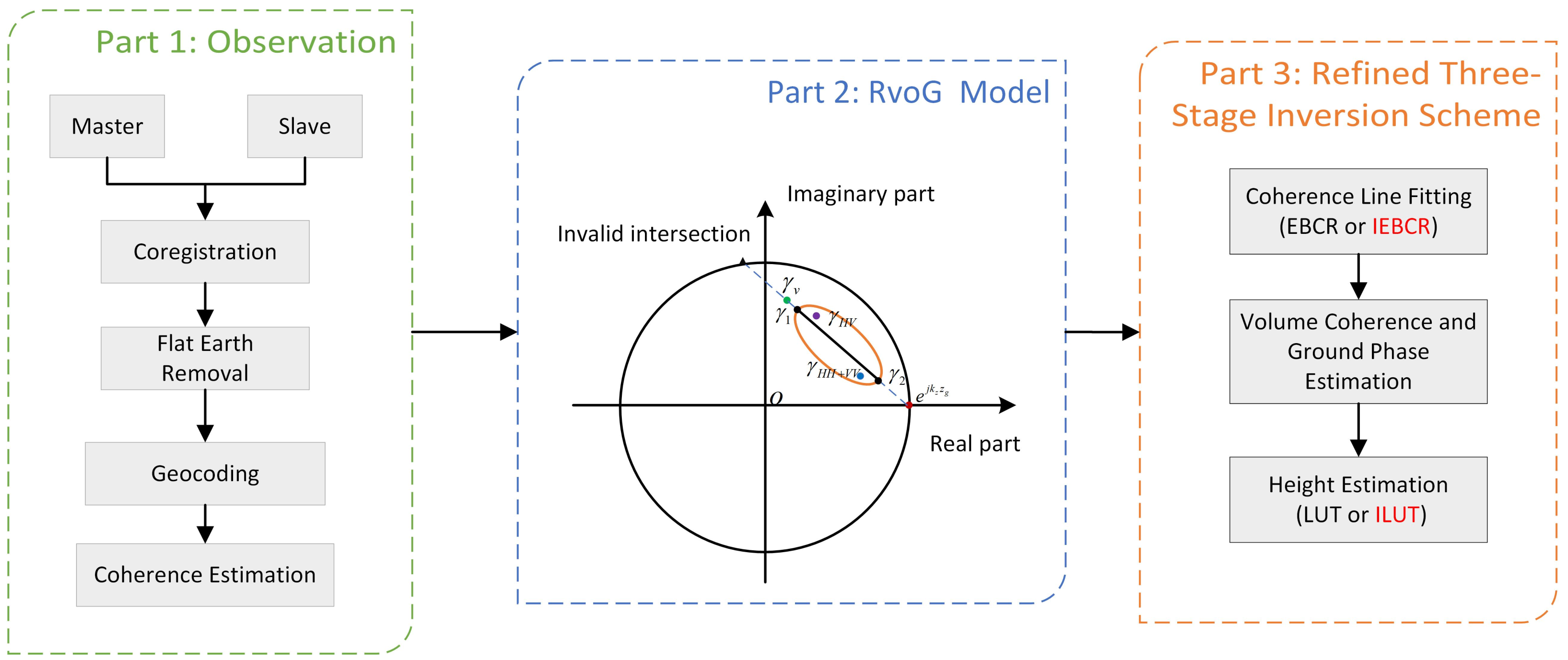
Figure 1. The PolInSAR flow. The figure in Part 2 depicts the geometrical interpretation of the RVoG model in the unit circle. The orange ellipse is the locus of BCR. The green, purple, blue, and red points are volume coherence, HV polarization coherence, HH+VV polarization coherence, and ground coherence, respectively. The black points denote two candidates of the volume coherence with the largest and smallest GVR, respectively. The blue dotted line linking γ v and e j k z z g is the theoretical distribution of coherence based on the RVoG model. The solid line over the blue dotted line is the visible segment. The black triangle is the invalid intersection.
Remotesensing 14 02438 g001
Figure 2. The example of the eigenvectors. U is the eigenvector matrix of T 1 A k and V is the eigenvector matrix of T 1 A k + 1 . The eigenvectors are the columns of U and V. The arrows denote the eigenvectors in the 3-D plot.
Remotesensing 14 02438 g002
Figure 3. The different sorting cases of eigenvalues.
Remotesensing 14 02438 g003
Figure 4. The RVoG function with θ = π / 4 , k z = 0.12 m 1 .
Remotesensing 14 02438 g004
Figure 5. Geometric interpretation of the second part of the RVoG function. The blue vector denotes e p 1 h v . After rotating a angle of k z h v , e p 1 h v becomes e p 1 h v + j k z h v denoted by the black vector. The red vector is 1 . The green vector presents e p 1 h v 1 . The orange vector denotes e p 1 h v + j k z h v 1 , which is the vector sum of e p 1 h v + j k z h v and 1 .
Remotesensing 14 02438 g005
Figure 6. The contour of the partial derivative of the RVoG function. k e ranges between 0 and 1 dB/m [14], and k z > 0.01 m 1 , θ = π / 4 . (a) Direction of h v . (b) Direction of p 1 .
Remotesensing 14 02438 g006
Figure 7. Different representation of the loss function with θ = π / 4 , k z = 0.12 m 1 . The red asterisks denote the location of the observed coherence which is also the optimal solution. The black rectangles indicate the neighborhood near the optimal solution. (a) Geometrical representation of the loss function. The area enclosed by the green line is the solution space where the coherences are calculated by Equation (6). The blue line denotes the direction of h v . The red line presents the direction of k e . (b) The contour of the loss function.
Remotesensing 14 02438 g007
Figure 8. The Pauli-basis color composite map and LiDAR H100 height map. Both maps are defined in the UTM Zone 34 coordinate. (a) The Pauli-basis color composite map. (b) The LiDAR H100 height map. The polygons are used in the forest height validation. The color ramp ranges from 0 to 35 m.
Remotesensing 14 02438 g008
Figure 9. The forest height inversion results of P-band in different configurations. The color ramps ranges from 0 to 35 m. (a) TSIA + EBCR + LUT. (b) TSIA + IEBCR + ILUT. (c) TSIA + EBCR + ILUT. (d) TSIA + IEBCR + LUT.
Remotesensing 14 02438 g009aRemotesensing 14 02438 g009b
Figure 10. The correlation plots of P-band in different configurations. (a) TSIA + EBCR + LUT. (b) TSIA + IEBCR + ILUT. (c) TSIA + EBCR + ILUT. (d) TSIA + IEBCR + LUT.
Remotesensing 14 02438 g010
Figure 11. The single baseline inversion results of L-band in different configurations. The color ramps = [0, 35] m. (a) TSIA + EBCR + LUT. (b) TSIA + IEBCR + ILUT. (c) TSIA + EBCR + ILUT. (d) TSIA + IEBCR + LUT.
Remotesensing 14 02438 g011
Figure 12. The correlation plots of L-band in different configurations. (a) TSIA + EBCR + LUT. (b) TSIA + IEBCR + ILUT. (c) TSIA + EBCR + ILUT. (d) TSIA + IEBCR + LUT.
Remotesensing 14 02438 g012
Figure 13. The absoulte difference of estimated height between TSIA + IEBCR + ILUT and TSIA + EBCR + ILUT. The color ramps range from 0 to 1.2 m. (a) P-band. (b). L-band. (c). The distribution of the absoulte difference.
Remotesensing 14 02438 g013
Figure 14. The average number of iterations in ERCR and IEBCR and the improved curve in efficiency.
Remotesensing 14 02438 g014
Figure 15. The absoulte difference of loss function between TSIA + IEBCR + ILUT and TSIA + IEBCR + LUT. (a) P-band. (b). L-band. (c). The distribution of the absoulte error.
Remotesensing 14 02438 g015aRemotesensing 14 02438 g015b
Figure 16. Comparison of the ratio of complexity between theoretical analysis and simulation. (a) First experimental configuration. (b) Second experimental configuration.
Remotesensing 14 02438 g016
Table 1. Characteristics of PolInSAR data.
BandLP
Centre Frequency1.300 GHz0.349 GHz
Spatial Baseline6, 12, 18, 24, 30 m8, 16, 24, 32, 40 m
Flight Direction 133 and 313
Easting size9561
Northing size9821
Easting Range437,061–446,881 m
Northing Range7,119,733–7,129,293 m
Geocoded Resolution1 m × 1 m
The coordinate system is the UTM Zone 34 coordinate.
Publisher’s Note: MDPI stays neutral with regard to jurisdictional claims in published maps and institutional affiliations.