Article

Characteristics of Greening along Altitudinal Gradients on the Qinghai–Tibet Plateau Based on Time-Series Landsat Images

1
Key Laboratory of Digital Earth Science, Aerospace Information Research Institute, Chinese Academy of Sciences, Beijing 100094, China
2
International Research Center of Big Data for Sustainable Development Goals, Beijing 100094, China
3
University of Chinese Academy of Sciences, Beijing 100049, China
4
School of Life Sciences, Faculty of Science, University of Technology Sydney, Sydney, NSW 2007, Australia
5
Institute of Land Surface System and Sustainable Development, Faculty of Geographical Science, Beijing Normal University, Beijing 100875, China
6
Geospatial Sciences Center of Excellence, Department of Geography & Geospatial Sciences, South Dakota State University, Brookings, SD 57007, USA
7
Institute of Applied Remote Sensing and Information Technology, College of Environmental and Resource Sciences, Zhejiang University, Hangzhou 310058, China
8
Ministry of Education Key Laboratory for Earth System Modelling, Department of Earth System Science, Tsinghua University, Beijing 100084, China
9
Institute of Atmospheric Physics, Chinese Academy of Sciences, Beijing 100029, China
*
Author to whom correspondence should be addressed.
Remote Sens. 2022, 14(10), 2408; https://doi.org/10.3390/rs14102408
Submission received: 31 March 2022 / Revised: 10 May 2022 / Accepted: 15 May 2022 / Published: 17 May 2022

Abstract

:
The Qinghai–Tibet Plateau (QTP) is ecologically fragile and is especially sensitive to climate change. Previous studies have shown that the vegetation on the QTP is undergoing overall greening with variations along altitudinal gradients. However, the mechanisms that cause the differences in the spatiotemporal patterns of vegetation greening among different types of terrain and vegetation have not received sufficient attention. Therefore, in this study, we used a Landsat NDVI time-series for the period 1992–2020 and climate data to observe the effects of terrain and vegetation types on the spatiotemporal patterns in vegetation greening on the QTP and to analyze the factors driving this greening using the geographical detector and the velocity of the vertical movement of vegetation greenness isolines. The results showed the following: (1) The vertical movement of the vegetation greenness isolines was affected by the temperature and precipitation at all elevations. The precipitation had a more substantial effect than the temperature below 3000 m. In contrast, above 3000 m, the temperature had a greater effect than the precipitation. (2) The velocity of the vertical movement of the vegetation greenness isolines of woody plants was higher than that of herbaceous plants. (3) The influence of slope on the vertical movement of vegetation greenness isolines was more significant than that of the aspect. The results of this study provided details of the spatiotemporal differences in vegetation greening between different types of terrain and vegetation at a 30-m scale as well as of the underlying factors driving this greening. These results will help to support ecological protection policies on the QTP.

1. Introduction

With an altitude averaging higher than 4000 m, the QTP, famous as the world’s ‘third pole’, is the highest plateau in the world [1,2]. The QTP is also known for its significant thermal and mechanical influences on the regional and global climate [2]. Compared to other regions at the same latitude, vegetation growth on the QTP is more vulnerable and sensitive to climate change due almost entirely to its topography [3,4]. In recent decades, many studies have indicated that the QTP has been undergoing significant warming and is becoming wetter [5,6,7]. These trends have been accompanied by overall vegetation greening [6,8,9]. The long-term change in vegetation greenness on the QTP is driven by climate change [8,10,11], particularly by the trend to warmer and wetter conditions [12]. The role of precipitation and temperature on QTP vegetation greenness shifts at 3000 m, and mismatch between vegetation greenness and temperature isolines shifts along elevation on the QTP has been reported by previous researchers [13,14]. However, these studies either focused on analyzing the elevation-dependent relationship between temperature and vegetation greenness or only analyzed vegetation greenness variations under climate change taking the QTP as a whole. It is urgent that this knowledge gap is filled, which will involve clarifying the variations in the spatiotemporal patterns of vegetation greening across different types of terrain and vegetation and underlying mechanisms.
Vegetation forms a vital connection between the pedosphere, atmosphere, and hydrosphere, and is one of the main components of the terrestrial ecosystem [15]. Vegetation greenness is a proxy for aboveground green biomass, the carbon and water cycles, energy flows, and other terrestrial ecosystem processes. Changes in vegetation greenness on the QTP significantly modify the biophysical properties of the land surface [13,16,17]. In previous studies, observations of the response of vegetation greenness on the QTP to climate change have been made from the perspectives of the spatial patterns and temporal variations in this response. The majority of the east Indian Himalayan region has seen a more greening trend than browning [18], with vegetation expansion [19,20]. The distribution of vegetation in the mountainous parts of the QTP often displays a clear relation to elevation, and clear changes with elevation have been found in the response of vegetation growth and greenness to climate change [21].
It is important to clarify the elevation-dependent relations between climate change and vegetation greenness in the mountainous parts of the QTP. Some studies have demonstrated the effect of temperature and precipitation changes along altitudinal gradients [16,22,23,24,25]. For example, Wang, et al. [14] found that the response of vegetation greenness to climate change varies with altitude and shifts at 2400 m. Some studies have inferred that a lag in the response of vegetation activity to temperature change or by limits on the availability of water or nutrients might cause the mismatch between climate warming and vegetation greening along altitudes above 3000 m on the QTP [13]. Other studies have shown that precipitation and temperature both have an effect on vegetation greening but with different intensities at different altitudes: for example, the precipitation has a stronger influence than temperature at lower elevations [14]. Similar results have been found from research on the vertical movement of vegetation greenness isolines in different mountainous regions using Landsat NDVI. These results showed that warming has different impacts on vegetation greenness isolines at different altitudes: vegetation greenness isolines are tending to move upward at higher altitudes and downward at lower altitudes [26].
Although elevation-dependent relationships between vegetation greenness change and climate change have been documented in some studies, the characteristics of vegetation greenness that are occurring in different types of terrain on the QTP and for different vegetation types have received little attention. The land surface is an important regulator of the energy budget and water availability, and the surface of the QTP is very complex. As a result, the land surface can have a critical impact on the regulation of vegetation dynamics [12,19]. For example, regions of vegetation change are mainly found where the slope is less than 20° and the elevation is in the range of 3000–5000 m. In particular, the response of the fraction of vegetation cover (FVC) to climate change is strongest at elevations of 3000–4000 m [27], and the changes of vegetation phenology under climate change differ as slope increases [28,29,30]. The vegetation type is also affected by the climate, soil, and terrain [31], and the spatiotemporal trends in vegetation greening vary greatly with vegetation type across the QTP [15,32]. For example, sufficient preseason precipitation may delay the emergence of evergreen forests in the southeastern part of the plateau while advancing the emergence in areas of alpine steppe, sparse alpine vegetation, or sparse alpine shrub in relatively arid areas [3]. In controlled experiments on the QTP, it has been observed that, in areas of alpine meadow, an increase in precipitation has a greater effect on vegetation greening than warming has [24,33]. Additionally, climate warming-induced changes in carbon and nutrient cycling may be more pronounced in drier alpine meadows than in wetter swamps [34]. Finally, interactions between different vegetation types can slow the upward movement of tree lines induced by climate warming [35], and time lags have also been observed between changes in climate variables and vegetation greenness in areas of alpine steppe, alpine meadow, and subalpine plain meadow [15,19].
Previous studies have enriched our understanding of the spatial variability in greening trends on the QTP. However, these studies were limited in some respects. First, the spatial resolution of the data used in these studies was poor; for example, GIMMS NDVI, MODIS NDVI, and gridded climate data have a spatial resolution of 8 km, 250 m, and 0.1°, respectively. These data are not appropriate for analyzing elevation-dependent vegetation phenomena because vegetated and non-vegetated areas can be mixed in coarse NDVI data [36]. Moreover, because in situ climate observations on the QTP are sparse, there may be gaps in the information needed to determine the details of the elevation-dependent variability of climate factors [6]. Additionally, earlier studies usually focused more on the impact of climate change on the greening trend and seldom examined the role of terrain and vegetation types. It is still important to clarify the mechanisms of vegetation greening across different terrain and vegetation types on the QTP. Vegetation indices (such as the NDVI) are surrogates for vegetation greenness and are widely used to monitor vegetation dynamics at regional and continental scales [37]. Therefore, in this study, the paper used a Landsat NDVI time-series for the period 1992–2020 and high spatial resolution climate data to investigate vegetation greening trends between different terrain and vegetation types on the QTP. The results of this study will help to ensure the ecological security of the QTP.

2. Materials and Methods
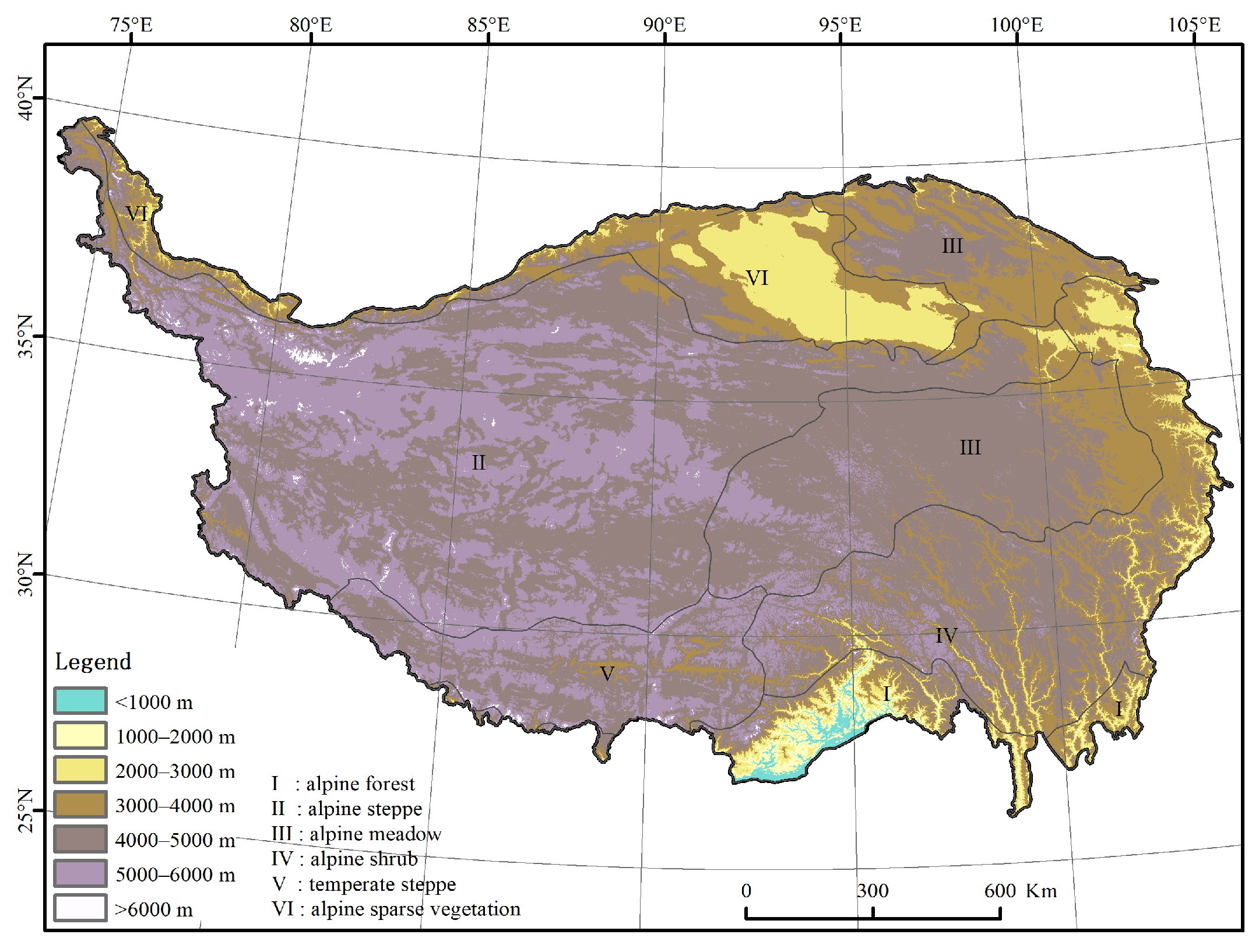
2.1. Study Region

The QTP region extents from 26.5° N to 39.5° N, 78.3° E to 103.1° E, with an average elevation higher than 4000 m (as shown in Figure 1). The average annual temperature varies from −15 to 10 °C, and the average annual precipitation varies from 392 to 764 mm. The main vegetation types in the QTP are alpine steppe (dominated by cushion plants), alpine meadow (dominated by perennial tussock grasses), and alpine shrub [25,32]. The focus of this research was on regions of vegetation. Therefore, pixels that had mean NDVIGS values of less than 0.1 for the period 1992–2020 were considered to be non-vegetation areas and were excluded from further analysis [13,16,26]. Pixels with observations made in each of the years 1992, 1994, 2000–2002, 2004–2011, and 2013–2020 were included in the analysis. The areas of vegetation thus generated were then taken as being the study area that is mainly located at the overlap area of neighboring Landsat orbits. The calculation below is located at this study area.

2.2. Preprocessing of Landsat Time-Series

The Landsat mission has provided an uninterrupted series of high-resolution remote sensing data for more than 40 years since the launch of the first satellite in the series in 1972. The first valid observations of the QTP were made in 1986; however, prior to the launch of Landsat 7 in 1999, the number of valid Landsat observations of the QTP was small. Because of the malfunction of the Landsat 7 scan-line corrector in May 2003 and the transmission failure suffered by the Landsat 5 Thematic Mapper (TM) in November 2011, the number of valid observations made in 2003 and 2012 was also small. Based on the number of available Landsat observations, we finally selected the years 1992, 1994, 2000–2002, 2004–2011, and 2013–2020—a total of 21 years—for analysis.
There are some inconsistencies between the Landsat TM, ETM+, and OLI records of the QTP. In order to make the data acquired by the different sensors comparable, we first adjusted the reflectance values of the Landsat 5 TM and Landsat 7 ETM+ data to match those of the Landsat 8 OLI data by using a linear transformation function [38]. In each dataset, we then masked areas of cloud, cloud shade, and snow by using a pixel-quality band generated by the CFMask algorithm [39]. In addition, because Landsat 5 scenes often contain abnormalities along the edges, which result in missing data and outlier NDVI values, we used a 450-m inward buffer to mask these abnormal pixels [40,41]. Following this processing, we calculated the NDVI values for each Landsat dataset by using the surface reflectances in the near-infrared and red bands; the counts of valid Landsat NDVI pixels are shown in Figure 2. From these, we calculated monthly NDVI values using the maximum value composite (MVC) method to remove the effects of atmospheric conditions, residual clouds, and aerosol scattering [42]. Based on the hypothesis that, over a brief period of time, the NDVI will change linearly [43], for months where data were missing due to cloud contamination, the gap was filled by linear interpolation between values of the adjacent months that had not been identified as cloudy [44,45]. Finally, the annual growing season NDVI (NDVIGS) was defined as the mean of the filtered maximum NDVI values across the five months May to September. All of this preprocessing of the Landsat data was performed on the Google Earth Engine (GEE) platform.

2.3. Climate Data

The climate dataset was provided by the National Earth System Science Data Center of the National Science and Technology Infrastructure of China (http://www.geodata.cn, accessed on 16 October 2021). The dataset included monthly precipitation and mean temperature data with a 1-km spatial resolution. The dataset was spatially downscaled from the 30′ Climatic Research Unit (CRU) time-series with WorldClim climatology dataset using the delta method and evaluated using observations made at 496 weather stations across China. This made the data suitable for climate change research in China by producing a dataset that had a higher quality and finer spatial resolution than the CRU data [46]. The annual growing season temperature (TGS) and annual growing season precipitation (PGS) were then defined as the mean of the monthly mean temperatures and the sum of monthly precipitation for the five months May to September. Finally, the PGS and TGS values were resampled to the resolution of the NDVI data using the bilinear interpolation method to standardize with Landsat NDVI.

2.4. Elevation and Vegetation Type Data

The elevation data were provided by the Advanced Spaceborne Thermal Emission and Reflected Radiometer Global Digital Elevation Model Version 2 (ASTER GDEM V2, https://earthexplorer.usgs.gov, accessed on 16 October 2021) and had a spatial resolution of 30 m. Information about the vegetation types on the QTP was extracted from the 1:1,000,000 Vegetation Atlas of China provided by the Resource and Environment Science and Data Center (https://www.resdc.cn/data.aspx?DATAID=122, accessed on 18 October 2021). The vegetation type data were resampled to the resolution of the NDVI data using the nearest-neighbor interpolation method.

2.5. Elevation Dependence of the Movement of Vegetation Greenness Isolines

In order to observe the elevation-dependent patterns in the movement of vegetation greenness isolines, we used the NDVI as a surrogate for the vegetation greenness to analyze the elevation-dependent relationship between (1) the NDVI of a pixel at a specific elevation or the average NDVI of all pixels within a specific elevation interval and (2) the altitude. At a regional level, the QTP was divided into 56,100-m elevation bins from the 200-m bin (150–250 m) to the 5700-m bin (5650–5750 m). We calculated the velocity of the vertical movement of the vegetation greenness isolines (V_NDVIGS(h), units: m/year) for each elevation bin using Equation (1):
V NDVI GS ( h ) = T NDVI GS ( h ) A NDVI GS ( h )
where T_NDVIGS(h) (units: year−1) is the temporal rate of change of NDVIGS, which is equal to the slope of the linear regression of the annual NDVIGS against the year. A_NDVIGS(h) (units: m−1) is the gradient (with elevation) of NDVIGS at the bin with elevation h; a positive A_NDVIGS(h) indicates that the value of NDVIGS is higher at higher elevations, a negative value indicates that NDVIGS is higher at lower elevations. A_NDVIGS(h) can be calculated using Equation (2):
A NDVI GS ( h ) = NDVI GS [ ( h 100 ) : h ] NDVI GS [ h : ( h + 100 ) ] E [ ( h 100 ) : h ] E [ h : ( h + 100 ) ]
where E[(h−100):h] is the mean elevation of all valid pixels in the bins with elevations h−100 and h, and NDVIGS[(h−100):h] is the mean value of NDVIGS for all valid pixels in the bins with elevations h−100 and h. E[h:(h+100)] and NDVIGS[h:(h+100)] are similarly defined.
At the pixel level, the velocity of the vegetation greenness isolines was determined using Equation (1), but based on individual pixels rather than bin averages. The temporal rate of change of NDVIGS for a given pixel was defined as the slope of the linear regression of the annual NDVIGS against the year. The method used for calculating the gradient was different from that used in the regional-level analysis. Within a 3 × 3 moving window, the gradient at the central pixel was defined as the ratio of the difference in NDVIGS to the difference in elevation along the line of steepest slope among the horizontal, vertical, and two diagonal directions [13,47]. Whether V_NDVIGS was positive or negative was determined by the signs of T_NDVIGS and A_NDVIGS: a negative V_NDVIGS indicated upward movement of the greenness isolines. There were two different ‘upward’ possibilities: ‘upward1’ (T_NDVIGS > 0 and A_NDVIGS < 0) and ‘upward2’ (T_NDVIGS < 0 and A_NDVIGS > 0). A positive V_NDVIGS indicated downward movement of the greenness isolines and corresponded to the two cases ‘downward1’ (T_NDVIGS < 0 and A_NDVIGS < 0) and ‘downward2’ (T_NDVIGS < 0, A_NDVIGS > 0) [14,21].

2.6. Factors Driving the Elevation-Dependent Movement of Vegetation Greenness Isolines

To analyze the factors driving the spatial heterogeneity of the vegetation greenness, we used the geographic detector (GD) [48,49] to quantitatively compare the effects of the elevation, slope, aspect, temperature, precipitation, and vegetation type on the multiyear average value of NDVIGS. The fundamental hypothesis behind the GD is that if an independent variable has an important influence on a dependent variable, then the spatial distribution of the independent and dependent variables should be similar. The value of the GD is in the range [0, 1]; the higher the value, the stronger the influence of the independent variable on the dependent variable [48]. In this study, independent variable are slope, aspect, elevation, vegetation type, and multiyear averages of TGS and PGS; the dependent variable is the multiyear average of the growing season NDVI (NDVIGS). The GD is defined as Equation (3):
GD = 1 h = 1 L N h σ h 2 N σ 2
where, in this study, h = 1, …, L is the stratum (category) of NDVIGS for the independent variable x, Nh and N are the numbers of samples in the stratum h and total samples in all categories, respectively, and σh2 and σ2 were the variances of NDVIGS in the stratum h and in all categories, respectively. The metric variables such as the elevation, slope, temperature, and precipitation were discretized using 100-m, 5°, 1 °C, and 100-mm intervals, respectively.
To analyze the impact of PGS and TGS on the vegetation greenness in the temporal dimension, for each pixel, we obtained the coefficients of PGS and TGS for the period 1992–2020 based on least-squares regression using Equation (4) [21]. To determine which factors were driving the temporal change in NDVIGS, the pixels were classified into four categories (Table 1) based on the sign of the trend in NDVIGS and the signs of the coefficients α and β in Equation (4). The four different categories were: (a) the trend in NDVIGS is primarily driven by the trend in TGS, (b) the trend in NDVIGS is primarily driven by the trend in PGS, (c) the trend in NDVIGS is mainly determined by the trend in both PGS and TGS, and (d) the trend in NDVIGS is possibly driven by other factors [21]. Equation (4) is written as:
NDVI GS = α × T GS + β × P GS + ε

3. Results

3.1. Changes in Spatiotemporal Patterns in Vegetation Greenness on the QTP

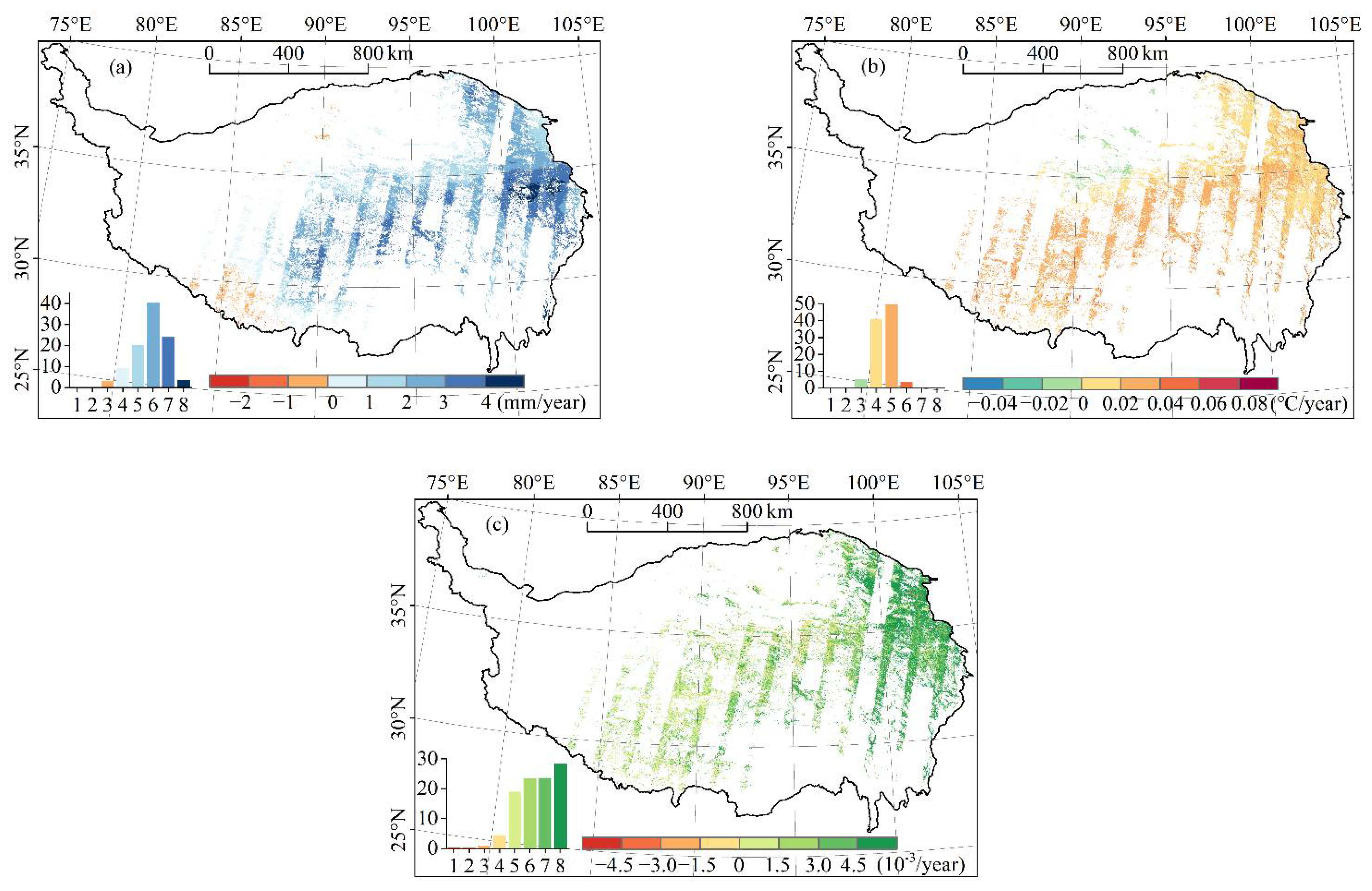
3.1.1. Temporal Trends in Vegetation Greenness, TGS, and PGS on the QTP

According to the temporal trends in PGS shown in Figure 3a, about 90% of the QTP study area became wetter over the study period. The rate of change of PGS is concentrated in the range 0–4 mm/year, with pixels where the rate of change is 2–3 mm/year accounting for 40% of all pixels. In most areas between 30° N and 35° N, the rate of change of PGS is greater than 3 mm/year, which means that the climate became considerably wetter. In the southwest of the QTP, east of 90° E and north of 35° N, there are two small areas where the rate of change of PGS is between −1 and 0 mm/year, which means that there was a drying trend. According to the temporal trends in TGS shown in Figure 3b, more than 90% of the QTP study area became warmer, with the rate of change concentrated in the range 0–0.06 °C/year and pixels corresponding to a rate of 0.02–0.04 °C/year accounting for nearly 50% of the total. In most areas between 30° N and 35° N, the temporal trends of TGS is in the range 0.02–0.04 °C/year, which means that the warming speed was relatively fast. Most areas north of 35° N and between 90° E and 95° E have a rate of change of TGS between −0.02 and 0 °C/year, which means that they became colder over the study period. According to the temporal trends in NDVIGS shown in Figure 3b, 90% of the QTP study area became greener. The rate of change of NDVIGS in most areas east of 100° E is greater than 4.5 × 10⁻³ year−1; in most other parts of the study area, it is between 0 and 3 × 10⁻³ year−1. From Figure 3, it can be seen that there is a region that became significantly warmer and wetter located between 30° N and 35° N. About 94% of the pixels in the QTP study area experienced greening, and there is a region of significant greening located east of 100° E. However, this does not match the region between 30° N and 35° N that is becoming noticeably warmer and wetter.

3.1.2. Spatiotemporal Variations in the Change in Vegetation Greenness on the QTP

Figure 4a shows that the temporal trends in NDVIGS, PGS, and TGS vary with elevation. The rate of change of NDVIGS fluctuates significantly between 0.004 and 0.0055 year−1 within 200 and 3500 m. The rate of change of NDVIGS decreases steadily from 0.0055 year−1 at 3500 m to 0.002 year−1 at 4800 m and remains at 0.002 year−1 between 4800 and 5300 m. It then decreases again to 0.001 year−1 at 5700 m. The rate of change of PGS declines as the elevation increases. More specifically, the rate of change of PGS fluctuates within the range 1.0–5.5 mm/year between 200 and 1200 m, decreases gradually from 5.0 mm/year at 1200 m to 1.5 mm/year at 2800 m, increases slightly from 1.5 mm/year at 2800 m to 3.0 mm/year at 3500 m, and then continually decreases from 3.0 mm/year at 3500 m to 0.0 mm/year at 5700 m. The rate of change of TGS fluctuates greatly within the range 0.01–0.27 °C/year between 200 and 1200 m and remains at 0.02 °C/year between 1200 and 2600 m. Above 3000 m, the rate of change of TGS tends to increase slightly and increases significantly from 0.02 °C/year at 5000 m to 0.04 °C/year at 5700 m. The rates of change of NDVIGS, PGS, and TGS all fall near 2800 m.
As shown in Figure 4b, at lower altitudes (200–3500 m), the vegetation greenness isolines alternate between moving up and moving down along elevation intervals. At higher altitudes (3500–5700 m), the motion is mainly upward. The patterns of vertical movement of the PGS and TGS isolines between 200 and 2600 m are similar and almost opposite to those of the NDVIGS isolines. Between 2600 and 3800 m, the patterns of vertical movement of the NDVIGS and PGS isolines are similar and almost opposite to those of the TGS isolines, indicating that the vertical movement of the NDVIGS isolines might be influenced by the movement of the PGS isolines. Above 3800 m, the vertical velocity of the NDVIGS isolines is stable with a somewhat similar trend to that of the TGS isolines; this similarity becomes stronger above 5000 m. The vertical velocity of the vegetation greenness isolines is generally about 20 m/year; the exceptions are near 500 m, 900 m, 1700 m, 3100 m, and 5200 m, where the absolute velocity is greater than 100 m/year, and between 2300 and 2500 m, where the absolute velocity is greater than 50 m/year.

3.2. Factors Driving Spatiotemporal Changes in Greenness on the QTP

To quantitatively analyze the effects of the slope, aspect, elevation, vegetation type, and multiyear averages of TGS and PGS on the spatial heterogeneity in vegetation greenness, respectively, the geographical detector (GD) for the multiyear average of the growing season NDVI (NDVIGS) was obtained using intervals of 100 m, 5°, 1 °C, and 100 mm for the elevation, slope, average TGS, and average PGS, respectively, using eight different aspect azimuth angles and six vegetation types. The GD for PGS, vegetation type, elevation, slope, aspect, and TGS are 0.57, 0.48, 0.42, 0.21, 0.14, and 0.13. The results show that the multiyear average of PGS has the highest GD and that PGS can explain 57% of the spatial heterogeneity in the vegetation greenness. The results also show that the vegetation type and elevation can explain 48% and 42% of the heterogeneity, respectively. The values of the GD for the slope, aspect, and multiyear average of TGS are low, indicating that these factors have relatively little influence on the spatial distribution of NDVIGS on the QTP.
According to Figure 5a, within every elevation bin, the proportion of pixels where the vertical movement of the vegetation greenness isolines is primarily affected by both the temperature and precipitation is high—over 60% in each case. However, the degree to which the temperature and precipitation affect the movement differs with the elevation. Between 3000 and 5700 m, the proportion of pixels primarily affected by the temperature is higher than that primarily affected by the precipitation. Conversely, between 200 and 3000 m, the proportion of pixels primarily affected by the precipitation is higher than that mainly affected by the temperature. The proportion of pixels affected by both the temperature and precipitation falls from 85% at 200 m to 25% at 1000 m, whereas the proportion of pixels primarily affected by the precipitation increases from about 10% at 200 m to nearly 40% at 1000 m. The proportion of pixels mainly affected by other factors increases from 10% at 200 m to nearly 35% at 1000 m. Above 1000 m, the proportion of pixels where the primary influence on the vertical movement of the greenness isolines is due to both temperature and precipitation increases sharply to about 80%, whereas the proportion of pixels mainly affected by other factors decreases rapidly and remains at between 0% and 5% at these elevations. The proportion of pixels affected by the temperature only increases from 10% at 3100 m to 25% at 4500 m, rapidly decreases from 25% at 4500 m to 10% at 5000 m, and then sharply increases again from 10% at 5000 m to 50% at 5700 m; it exceeds the proportion of pixels that are mainly affected by both the temperature and precipitation at 5500 m. Close to the 1000-m and 2800-m elevation bins, the proportions of pixels primarily affected by the temperature and by other factors both increase significantly, whereas there is no obvious change in the proportion of pixels mainly affected by the temperature only.
According to Figure 5b, 75.24% of the pixels in the QTP study region are primarily affected by both the temperature and precipitation; 13.24% are primarily affected by the temperature—these are found mainly in the eastern (102° E–103° E, 31° N–32° N), east-central (95° E–100° E, 33° N–35° N), and southwestern (83° E–86° E, 28° N–30° N) parts of the study area, where the vegetation types mainly include alpine shrub meadow, alpine meadow, and temperate steppe, and 9.36% of the pixels in the region are mainly affected by the precipitation—these are located mainly in the north-central (90° E–95° E, 34° N–40° N) and southwestern (86° E–90° E, 28° N–29° N) parts of the study area, where the vegetation types mainly include temperate shrub, alpine steppe, and temperate steppe. In 2.16% of the study area, the main effect on the vertical movement of the vegetation greenness isolines is due to other factors, and there are no obvious patterns in the spatial distribution of these pixels.

3.3. The Influence of the Terrain on the Vertical Movement of Vegetation Greenness

According to Figure 6a, the temporal trend in NDVIGS is not significantly affected by aspect. The average for all temporal rate of change in NDVIGS is between 0.0030 and 0.0035 year−1, the average value for all negative temporal rate of change in NDVIGS is between −0.0010 and 0.0015 year−1 for all aspects, and the average value for all positive temporal rate of change in NDVIGS is about 0.0035 year−1.
According to Figure 6b, the vertical velocity of the vegetation greenness isolines is the highest at an aspect of 315°: the average value for all positive vertical velocity of the vegetation greenness isolines is 18 m/year, and the average value for all negative vertical velocity of the vegetation greenness isolines is −17 m/year. The difference in velocity between positive and negative pixels is the lowest at an aspect of 180°: the mean value for all positive pixels is 12 m/year, and the mean value for all negative pixels is −11 m/year. Overall, the vertical velocity of the vegetation greenness isolines is small and negative for all eight values of the aspect azimuth at about −1 m/year.
According to Figure 6c, the factors driving the vertical movement of the vegetation greenness isolines differ significantly at the eight different aspect azimuths. For all eight different azimuth angles, among the four different groups of driving factors, the proportion of pixels mainly affected by both the temperature and precipitation is the highest at 75–76%, whereas the proportion of pixels primarily affected by other factors is the lowest and accounts for only 2–3%. The proportion of pixels primarily affected by either only the temperature or the precipitation is between 7% and 16%. The proportion of pixels primarily affected by the temperature is larger than that primarily affected by the precipitation at all of the different aspect azimuths except 90°; the difference between these two proportions is maximum at an aspect of 270°, where the difference is about 9%.
According to Figure 6d, the direction of motion of the vegetation greenness isolines is ‘upward1’ for about 51% of pixels and ‘downward2’ for about 44% of pixels; the proportions of ‘upward2’ and ‘downward1’ pixels are much lower, both accounting for about 2–3% of pixels. There is no significant overall difference between the proportions of pixels corresponding to upward and downward movement of vegetation greenness isolines: the difference is 9% at aspects of 45° and 225° and 5% at an aspect of 315°.
Then, we continue to discuss the slope’s impacts on the spatiotemporal changes in vegetation greenness on the QTP. According to Figure 7a, the mean temporal rates of change of NDVIGS for all pixels (0.003–0.0045 year−1) and all positive pixels (0.0032–0.0049 year−1) increase as the slope increases; the mean temporal rate of change of NDVIGS for all negative pixels increases from −0.0015 year−1 at a slope of 0° to −0.0010 year−1 at slope of 35°; it then gradually decreases to −0.0020 year−1 for steeper slopes.
According to Figure 7b, for all pixels, the mean value of the vertical velocity of the vegetation greenness isolines is about −2 m/year; the absolute mean value of the vertical velocity for both positive and negative pixels increases gradually from ±5 m/year to ±65 m/year with increasing slope, from a slope of 0° to a slope of 60°, indicating that the patterns of vertical motion of the vegetation greenness isolines become more complex as the slope increases.
According to Figure 7c, for each 5° slope bin, there are significant differences in the factors driving the vertical movement of the vegetation greenness isolines. For all slope bins, the proportion of pixels mainly affected by both the temperature and precipitation is greater than the proportions in the other categories and is around 73–77%. In all slope bins, the percentage of pixels primarily affected by other factors is the lowest among the four driving-factor categories and accounts for only 2–3% of pixels. The proportion of pixels primarily affected by the temperature gradually decreases from 14% to 10% as the slope increases from a slope of 0° to a slope of 60°. The proportion of pixels primarily affected by the precipitation decreases slightly from 10% at a slope of 0° to 9% at a slope of 25° and then increases from 9% to 15% as the slope increases from 25° to 60°. For slopes in the range 0°–40°, the proportion of pixels primarily affected by the temperature is larger than the proportion primarily affected by the precipitation; however, the opposite is true for slopes in the range of 40°–60°.
According to Figure 7d, in most cases, the direction of the vertical movement of the vegetation greenness isolines is in the upward1 (47–55%) or downward2 (41–47%) categories; the proportions of upward2 and downward1 pixels are both relatively small at around 2–3%. As the slope increases, the proportion of upward1 pixels increases rapidly from 47% at a slope of 0° to 55% at a slope of 35°; it then slowly falls to 52% at a slope of 60°. The proportion of downward2 pixels decreases rapidly from 47% at a slope of 0° to 41% at a slope of 35°; it then rises slowly to 44% at a slope of 60°. The proportion of upward1 pixels is higher than that of downward2 pixels in all the slope bins; the greatest difference (14%) occurs at a slope of 35°.

3.4. Variation in the Vertical Movement of Vegetation Greenness Isolines with Vegetation Types

The steepness of the slope has an obvious effect on the distribution of the vegetation types (Figure 8). Alpine steppe, alpine meadow, alpine sparse vegetation, and temperate steppe (vegetation types II, III, IV, and V, all consisting of mainly herbaceous plants) are mainly found in flat regions with slopes in the range of 10°–15°. Alpine forest and alpine shrub (vegetation types I and VI, all consisting of mainly woody plants) are mainly found in steeper regions with slopes in the range of 20°–30°.
The temporal rate of change of NDVIGS and the vertical velocity of the vegetation greenness isolines differ significantly for different vegetation types. For all vegetation types, NDVIGS shows an increasing trend, with rates of 0.002–0.005 year−1. The rate of increase of NDVIGS and the vertical velocity of the vegetation greenness isolines is highest for alpine forest (vegetation type I); the ranges of these values are also large. The mean temporal rates of change of NDVIGS for positive and negative alpine forest are 0.005 and −0.003 year−1, respectively; the mean velocities of the positive and negative pixels are 40 and −40 m/year, respectively, indicating that the greenness of this vegetation type may be affected by many factors. The temporal rate of change of NDVIGS and the velocity of the vertical movement of the vegetation greenness isolines for alpine meadow and alpine shrub (vegetation types III and VI) are lower, and the ranges of values small. The mean temporal rate of change of NDVIGS for all positive and negative pixels is in the range of 0.002–0.003 and −0.0005–−0.001 year−1, respectively, and the mean velocity for all positive and negative pixels is in the range of 5–10 and −5–−10 m/year, respectively (Figure 9a,b).
The factor driving the vertical movement of the vegetation greenness isolines differs significantly according to the vegetation type, Figure 9c. For all vegetation types, the proportion of pixels primarily affected by both the temperature and precipitation is the highest among the four driving-factor categories and is in the range of 62–82%; pixels primarily affected by other factors constitute the lowest proportion (0–3%) for all vegetation types. The proportion of pixels mainly affected by temperature is higher than that mainly affected by precipitation in the case of alpine meadow, alpine sparse vegetation, and alpine shrub (vegetation types III, IV, and VI) This indicates that the greenness of these three types of vegetation is sensitive to temperature; this is especially true of alpine sparse vegetation (vegetation type IV), with 24% of pixels being mainly affected by temperature. The proportion of pixels mainly affected by precipitation is higher than that mainly affected by temperature for alpine steppe, temperate steppe, and alpine shrub (vegetation types II, V, and VI), which indicates that the greenness of these three types of vegetation is sensitive to precipitation.
According to Figure 9d, the direction of the vertical movement of the vegetation greenness isolines for alpine shrub (vegetation type VI) is mainly in the categories upward1 (54% of pixels) and downward2 (44%), with a maximum difference of 10% between the two. The proportions of upward2 and downward1 pixels corresponding to this vegetation type are small (about 4% each). For alpine steppe (vegetation type II), the proportions of upward1 and downward2 pixels are both about 47%. For alpine sparse vegetation (vegetation type IV), the proportions of upward1 and downward2 pixels are 51% and 40%, respectively—a difference of 11%—and the proportions of upward2 and downward1 pixels are the lowest among all vegetation types at about 2% each. The highest absolute values of the vertical velocity of the vegetation greenness isolines are for alpine steppe, alpine sparse vegetation, and temperate steppe (vegetation types II, IV, and V), which indicates that these three categories of herbaceous alpine plants have a greater ability to adapt to climate change on the QTP.

4. Discussion

4.1. Characteristics and Causes of the Vertical Movement of Vegetation Greenness Isolines

The results described above show that the proportion of pixels in the QTP study area where the velocity of the vertical movement of the vegetation greenness isolines is affected by both temperature and precipitation exceeded 60% in all elevation bins (Figure 5a), which indicates that the change in vegetation greenness is influenced by the temperature and precipitation together rather than a single climate factor [8,10,11,14]. The size of the effect of the temperature and precipitation varied with the elevation. When the amount of precipitation met the maximum limit of the vegetation’s demand for water, the temperature had a greater effect than the precipitation; when the temperature reached the maximum limit that the vegetation can tolerate, the precipitation had a greater effect than the temperature [23,50].
The results also show that the influence of the precipitation on the vertical movement of the vegetation greenness isolines in the QTP study area is greater than that of the temperature at lower altitudes (200–3000 m), whereas the influence of the temperature is greater at higher altitudes (3000–5700 m). In previous research, it was also observed that the vertical movement of vegetation greenness isolines on the QTP was mainly affected by precipitation below 2400 m and by temperature above 2400 m [14]. The authors of these earlier studies considered that this difference was due to the large difference in the spatial resolution between NDVI and climate data. The vegetation type changes from alpine steppe-meadow at 4390–4500 m to alpine meadow at 4600–5210 m [51]. In our results, we found that, between 4500 and 5000 m, the proportion of pixels where the temperature plays the most important role in the vegetation greenness change dropped rapidly from 25% to 10%; the proportion of pixels where the vegetation greenness change is affected by both the temperature and precipitation increased rapidly from 60% to 80% (Figure 5a). The rate of change of TGS remained at 0.02 °C/year throughout this interval, and NDVIGS and PGS had similar decreasing trends (Figure 4a). Under these conditions, although the altitude is high, the vegetation greenness change is still affected by both the temperature and precipitation and not mainly by the temperature alone [23,51]. In addition, it is possible that terrain-induced temperature inversions in the period before the growing season [52] and the increasing non-growing season albedo [53] at elevations of 4500–5500 m are also factors that contribute to the rapid drop in the proportion of pixels mainly affected by temperature between 4500 and 5500 m.
Above 5000 m, the temporal rate of change of TGS increased with elevation (Figure 4a); this is consistent with the conclusion of previous research that the QTP is undergoing faster warming at high altitudes [54,55,56]. Meanwhile, the proportion of pixels where the vegetation greenness change is mainly affected by the temperature increased rapidly from 10% at 5000 m to 50% at 5700 m and exceeded that of pixels where the change is affected by both the temperature and precipitation (Figure 5a). These two results demonstrate that the vegetation greenness change is mainly controlled by the temperature above 5000 m [13]. On the QTP, the zone of maximum precipitation is around 5000 m [52], and the temporal rate of change of PGS fell with increasing altitude above 5000 m (Figure 4a). Most regions at 5000 m above sea level are located near the lower limit of permafrost [52], and alpine tree lines on the QTP do not reach 5000 m [57]. Above this level, the main vegetation types on the QTP are alpine meadow and alpine cushion, and these are sensitive to temperature change [58,59]. A significant decrease in the temporal trend of NDVIGS (Figure 4a) and aboveground biomass [60,61] was also found as the elevation above 5000 m increased. A significant acceleration in warming and a stable temporal trend in PGS were observed at high elevations within the permafrost region. These were the primary reasons for the observed rapid increase in the proportion of pixels where the vegetation greenness change is mainly affected by temperature above 5000 m on the QTP.

4.2. Differences in the Vertical Movement of Vegetation Greenness Isolines between Different Types of Terrain and Vegetation

The vertical movement of vegetation greenness isolines was found to differ according to the gradient; differences in the spatiotemporal variations in vegetation greenness on the QTP were also found for different types of terrain and vegetation. The conclusion that the slope affects the vertical movement of vegetation greenness isolines more than the aspect does is consistent with the findings of An et al. [13] and Lu et al. [26], who also observed that there was no significant difference in the velocity of the vertical movement of vegetation greenness isolines on the QTP at different aspects. There was also a study revealing that vegetation greening trends at lower elevations occurred on steeper slopes, whilst at higher elevations, flatter areas exhibited stronger trends [19]. The value of the geographical detector (GD) for the slope was 0.21—greater than the value of 0.14 found for the aspect. No significant differences were found between the temporal rate of change of NDVIGS and the vertical velocity of the vegetation greenness isolines for different aspects. However, significant differences were found for different slope angles (Figure 6 and Figure 7), which supports the idea that the slope has a greater impact than the aspect. We found that the proportion of upward1 pixels increased with increasing slope, reaching a maximum at a slope of 35°. The relative influences of PGS and TGS on the vertical movement of vegetation greenness isolines changed at a slope of 35°. Lu et al. [26] observed that the velocity of the vertical movement of vegetation greenness isolines on the QTP increased with increasing slope and reached a maximum at a slope of 30°. This is similar to our conclusion—the slight difference may be caused by differences in the time span and in the spatial resolution of the data used in the two analyses.
How is it possible, then, that the vertical movement of the vegetation greenness isolines on the QTP is greatly affected by the slope but only slightly affected by the aspect? The terrain is a significant regulator of the availability of water, energy, and radiation at fine scales [12], and thus affects the distribution of vegetation types [31]. For example, on the QTP, areas of alpine shrub are mainly located in the southeast of the region at elevations of 3800–4800 m and on sunlit slopes; alpine meadow is mainly found in the east of the region at elevations of 4000–5000 m and on shaded slopes. Alpine grassland, which is adapted to a cold, dry climate is mainly found on the Chang Tang Plateau, the eastern part of the Kunlun Mountain plain, and around the headwaters of the Yangtze River at heights of 4200–5300 m [24,59]. Terrain features such as the slope and aspect determine the soil types that are present by influencing the rock-weathering process; they also affect the soil thickness by influencing the amount of soil erosion. As a result, specific vegetation types are associated with specific types of terrain. For example, within the QTP study area, herbaceous vegetation types such as alpine meadow, alpine grassland, and alpine sparse vegetation are mainly found in relatively flat areas with slopes of between 10° and 15°; woody plant types such as subalpine woodlands and shrubs are mainly found in steeper areas with slopes of between 20° and 30° (Figure 8). These observations confirm that the influence of the slope on the vertical movement of vegetation greenness isolines in the QTP study area is greater than that of the aspect and that the observed differences in the vertical movement of the vegetation greenness isolines associated with different types of terrain are, in fact, due to the different types of vegetation that occur there. The question then is, what differences are there in the patterns of vertical movement of vegetation greenness isolines on the QTP between different vegetation types?
We found that it is the availability of water and heat as well as differences in the sensitivity of different vegetation types to climate change that produced the differences in the vertical movement of vegetation greenness isolines for different vegetation types [23,50]. For example, in the northern part of the alpine forest in the east of the QTP study area, which is becoming colder and wetter, the change in vegetation greenness (102° E–103° E, 31° N–32° N) was mainly affected by TGS, whereas alpine grassland in the center of the northern part of the study area (90° E–95° E, 34° N–40° N) were mainly affected by PGS (see Figure 3 and Figure 5b). The east-central part of the QTP study area (95° E–100° E, 33° N–35° N) is becoming warmer and wetter; here, it was found that the change in the greenness of the alpine shrub and alpine meadow were mainly affected by TGS. Another region that is becoming warmer and wetter is the southwest of the study area (86° E–90° E, 28° N–29° N), where the results showed that the temperate grassland was mainly affected by PGS. The factors driving the vertical movement of vegetation greenness isolines differ significantly between different vegetation types (see Figure 9c). The proportion of pixels mainly affected by TGS was higher than that mainly affected by PGS in areas of alpine shrub, alpine meadow, and alpine sparse vegetation, indicating that changes in vegetation greenness for those species are more sensitive to temperature. The proportion of pixels mainly affected by PGS was higher than that mainly affected by TGS for alpine shrub and alpine steppe, indicating that changes in vegetation greenness for those species are more sensitive to precipitation. It has also been documented in earlier studies [12,13,20,33,35,62] that the changes in the greenness of alpine steppe and alpine shrub are more sensitive to precipitation, whereas for alpine forest and alpine meadow they are more sensitive to temperature. The main reasons for this are that alpine steppe and alpine shrub are greener and better adaptable to the environment. Alpine steppe is mainly found in flat areas above 4500 m, where the temperature is higher than in areas of alpine meadow. As a result, the alpine steppe is more sensitive to precipitation, whereas the alpine meadow is more sensitive to temperature as heat is less accessible to it.

4.3. Limitations of the Study and Future Prospects

There are clearly still some limitations to the analysis that was performed in this study. Firstly, because of the limited quality of the remote sensing data that were available, the study area was spatially discontinuous. Before the launch of Landsat 7 in 1999, the number of valid Landsat observations of the QTP was limited. As the cloud and shadow pixels were also masked, there were many missing pixels in the time-series of Landsat data, and these were randomly distributed in space. We used MODIS data to extract vegetated regions as a reference [13,14,26] and determined the proportion of valid Landsat pixels’ area in the reference vegetation region for the period 1987 to 2020. In order to ensure the reliability of the analysis and maximize the utilization of the time-series of Landsat data, annual NDVIGS values were calculated for the years 1992, 1994, 2000–2002, 2004–2011, and 2013–2020, for which the proportion of valid pixels was greater than 70% (Figure 10). In addition, the proportions of pixels in the study area corresponding to different terrain and vegetation types and altitudes were similar to those in the reference region (Figure 11). Therefore, although the study area in this paper was discontinuous, the pixels were evenly distributed across different terrain and vegetation types and altitudes, which means that the subsequent analysis was reliable.
Secondly, in the analysis of the factors that drive the temporal variations in the vegetation greenness isolines, the number of variables used was limited. We analyzed the effects of TGS, PGS, and other factors on the temporal variations in the vegetation greenness. However, some studies [32,34,35,63] have shown that radiation, length of daylight, land-use change, topography, and interactions between species—which were categorized as other factors in this study—also have a significant impact on vegetation greenness change in addition to the temperature and precipitation. What is more, whether changes in river-flows caused by snowmelt under climate warming could affect vegetation greenness is also worth researching [64].
Thirdly, the geographical detector has already been applied to consider the linear and nonlinear interactions between variables in the analyses of the factors driving the spatial heterogeneity in vegetation greenness on the QTP [26]. The analysis of the temporal heterogeneity that was performed in this study was based on binary linear regression, which could only analyze the linear interactions between variables. However, previous research has indicated that the effects of temperature and precipitation on vegetation greenness change on the QTP are nonlinear and complex [14,32,65]. Furthermore, the authors of these studies considered that the development of advanced data-processing methods to acquire a spatiotemporally seamless series of Landsat data to support sustainable development goals [66], and integrating the climate, terrain, radiation, vegetation type, and other variables to analyze the linear and nonlinear interactions between them, was required to improve the analysis of vegetation greenness changes on the QTP.

5. Conclusions

In this study, we used a time-series of 30-m Landsat NDVI data and 1-km climate data from 1992 to 2020 to observe long-term changes in the spatiotemporal patterns of vegetation greenness and variations in the response of vegetation greenness to climate change for different types of terrain and vegetation. The main conclusions of this study are as follows.
(1)
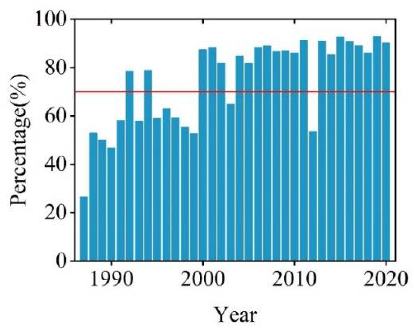
Over 90% of the QTP study area, the vegetation greenness has been increasing. The regions with the fastest rate of vegetation greenness increase do not match the regions that are clearly becoming warmer and wetter.
(2)
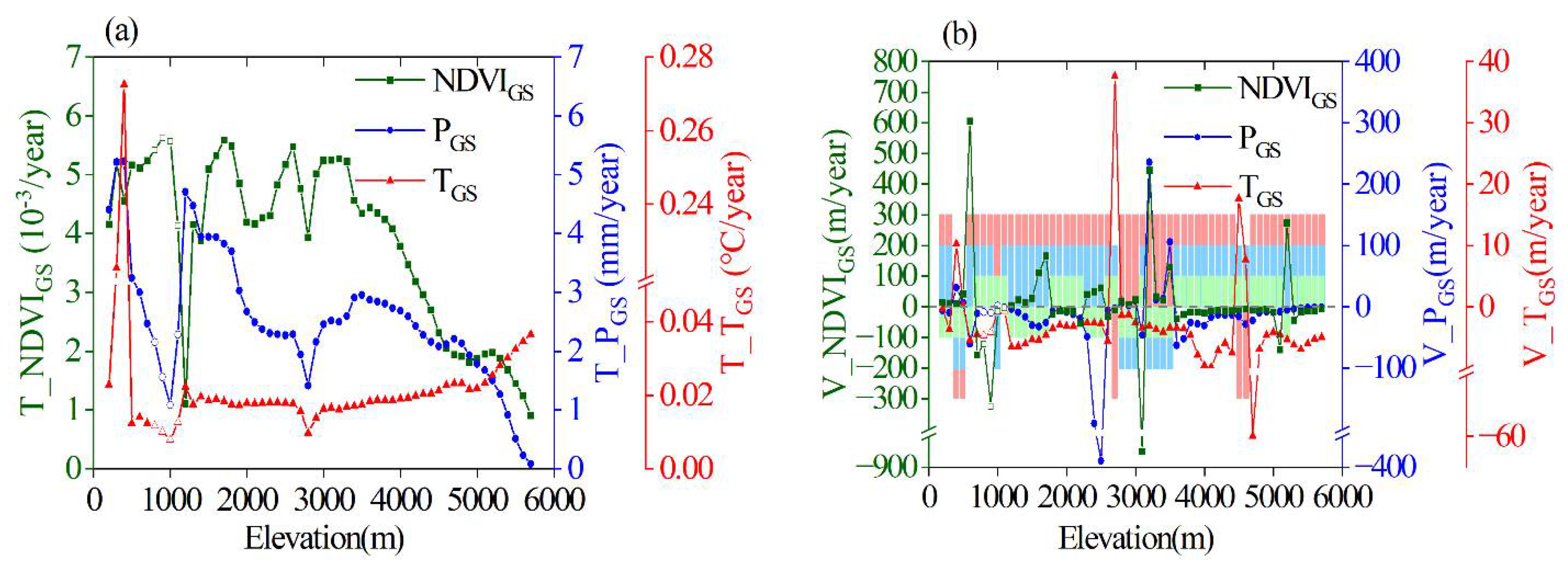
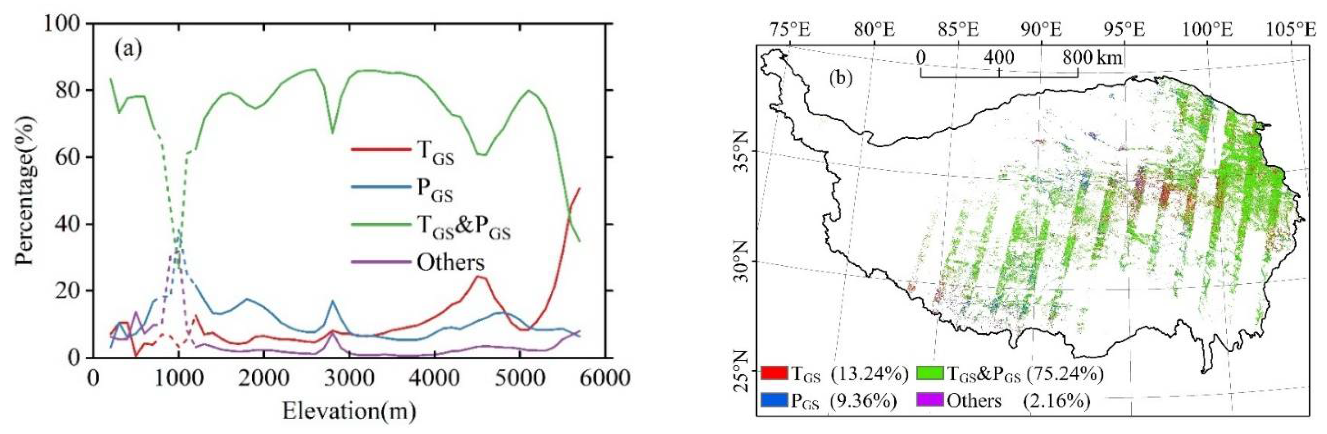
The vertical movement of vegetation greenness isolines is affected by both the temperature and precipitation between 200 and 5700 m. Precipitation plays a more important role at lower altitudes (200–3000 m), whereas, at higher altitudes (3000–5700 m), temperature plays a more important role.
(3)
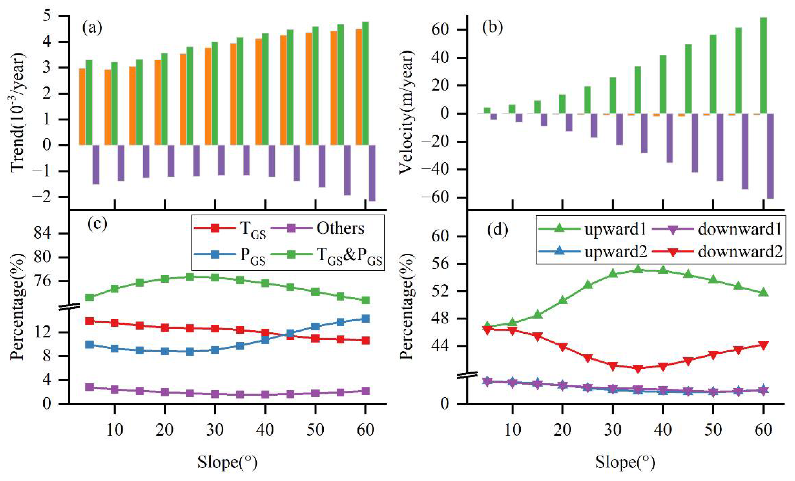
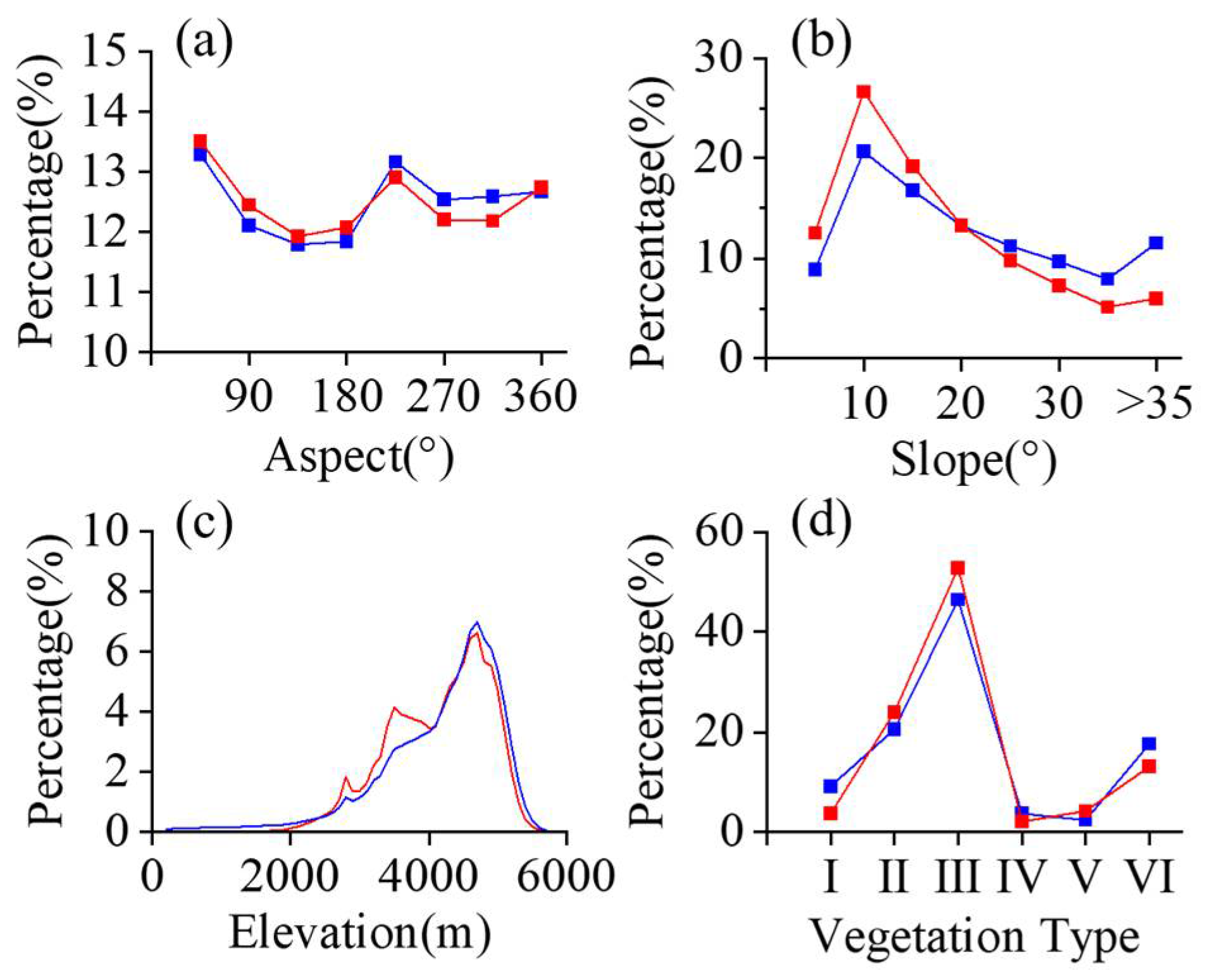
The terrain has notable impacts on the spatiotemporal changes in vegetation greenness on the QTP, with the effect of the slope being greater than that of the aspect.
(4)
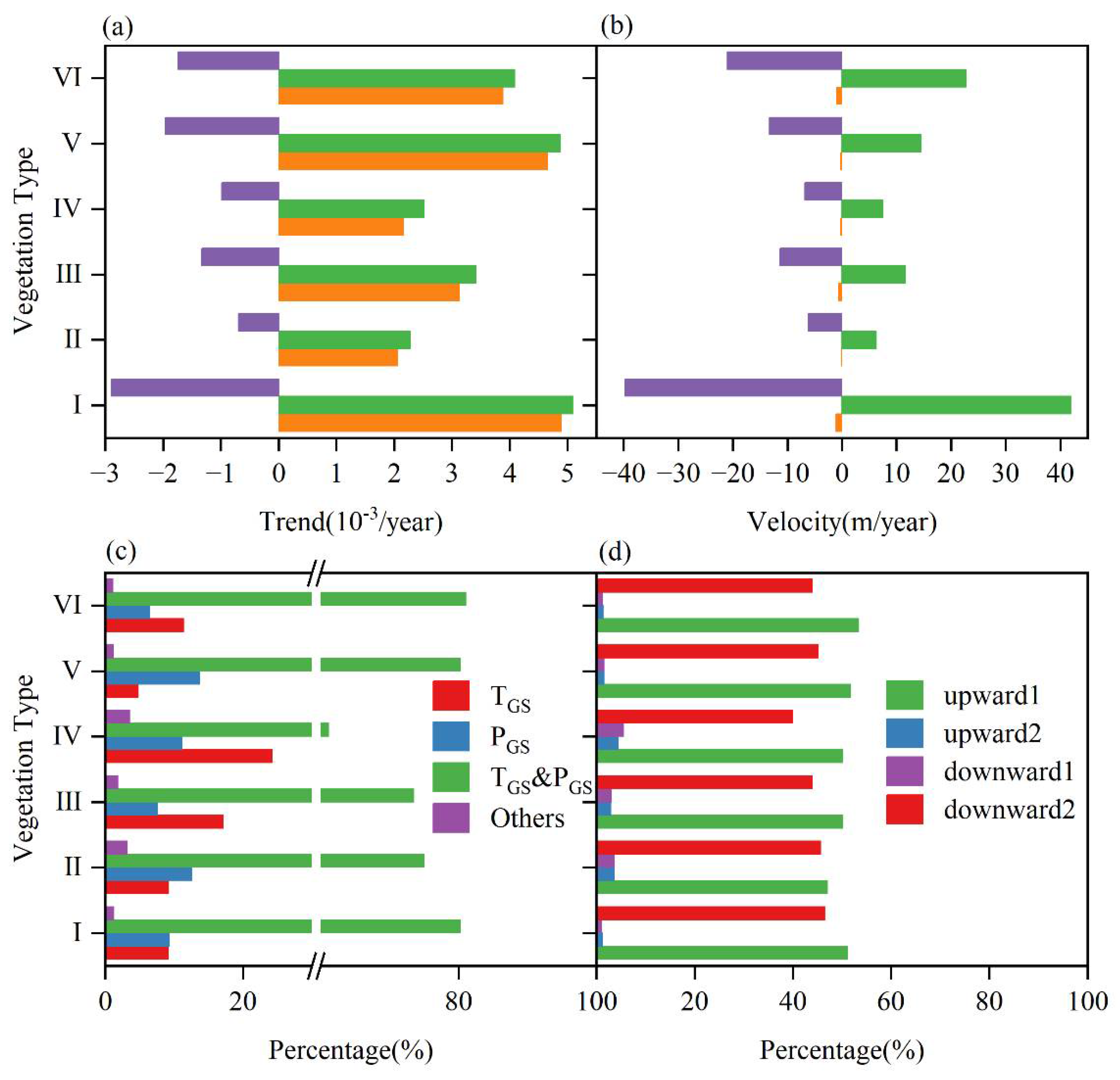
In the QTP study area, herbaceous vegetation types are mainly found in relatively flat areas, whereas woody plants are mainly found in relatively steep areas. The change in the greenness of subalpine broadleaf deciduous scrub, alpine meadow, and alpine sparse vegetation is more sensitive to temperature, while for subalpine needleleaf evergreen scrub and alpine grassland it is more sensitive to precipitation. The vertical velocity of the vegetation greenness isolines is higher for woody plants than for herbaceous plants, which means that the former are more adaptable to climate change.
These results enrich the understanding of differences in vegetation greening and the underlying factors for different types of terrain and vegetation at a spatial scale of 30 m and will help provide support to ecological protection on the QTP.

Author Contributions

Y.P., conceptualization, methodology, investigation, formal analysis, visualization, writing—original draft, writing—review and editing; Y.W., investigation, software; S.Z., software, visualization; A.R.H., writing—review and editing; M.S., conceptualization, writing—review and editing; X.Z., writing—review and editing; J.H., funding acquisition; G.H., project administration, funding acquisition; L.Y., resources; X.X., resources; Q.X., resources; D.P., supervision, writing—review and editing, project administration, funding acquisition, resources. All authors have read and agreed to the published version of the manuscript.

Funding

This research was funded by the Second Tibetan Plateau Scientific Expedition and Research Program, grant number 2019QZKK0307; the National Natural Science Foundation of China, grant number 42071329; the Strategic Priority Research Program of the Chinese Academy of Sciences, grant number XDA19070203; and the Erasmus+ Project, grant number 598838-EPP-1-2018-EL-EPPKA2-CBHE-JP.

Data Availability Statement

The climate dataset is available at http://www.geodata.cn. The elevation data is available from https://earthexplorer.usgs.gov. The vegetation types data is available at https://www.resdc.cn. The landsat data is available at https://code.earthengine.google.com. The datasets generated during the current study are available from the corresponding author on reasonable request. (All accessed on 30 March 2022).

Conflicts of Interest

The authors declare no conflict of interest.

References

  1. Wang, Q.; Hong, D. Understanding the plant diversity on the roof of the world. Innovation 2022, 3, 100215. [Google Scholar] [CrossRef] [PubMed]
  2. Duan, A.; Wu, G.; Liu, Y.; Ma, Y.; Zhao, P. Weather and climate effects of the Tibetan Plateau. Adv. Atmos. Sci. 2012, 29, 978–992. [Google Scholar] [CrossRef]
  3. Cheng, M.; Jin, J.; Zhang, J.; Jiang, H.; Wang, R. Effect of climate change on vegetation phenology of different land-cover types on the Tibetan Plateau. Int. J. Remote Sens. 2017, 39, 470–487. [Google Scholar] [CrossRef]
  4. Duan, J.; Esper, J.; Buntgen, U.; Li, L.; Xoplaki, E.; Zhang, H.; Wang, L.; Fang, Y.; Luterbacher, J. Weakening of annual temperature cycle over the Tibetan Plateau since the 1870s. Nat. Commun. 2017, 8, 14008. [Google Scholar] [CrossRef] [Green Version]
  5. Kuang, X.; Jiao, J.J. Review on climate change on the Tibetan Plateau during the last half century. J. Geophys. Res. D Atmos. JGR 2016, 121, 3979–4007. [Google Scholar] [CrossRef]
  6. Yao, T.; Xue, Y.; Chen, D.; Chen, F.; Thompson, L.; Cui, P.; Koike, T.; Lau, W.K.M.; Lettenmaier, D.; Mosbrugger, V.; et al. Recent Third Pole’s Rapid Warming Accompanies Cryospheric Melt and Water Cycle Intensification and Interactions between Monsoon and Environment: Multidisciplinary Approach with Observations, Modeling, and Analysis. Bull. Am. Meteorol. Soc. 2019, 100, 423–444. [Google Scholar] [CrossRef]
  7. Zhang, C.; Tang, Q.; Chen, D. Recent Changes in the Moisture Source of Precipitation over the Tibetan Plateau. J. Clim. 2017, 30, 1807–1819. [Google Scholar] [CrossRef]
  8. Zhu, Z.; Piao, S.; Myneni, R.B.; Huang, M.; Zeng, Z.; Canadell, J.G.; Ciais, P.; Sitch, S.; Friedlingstein, P.; Arneth, A.; et al. Greening of the Earth and its drivers. Nat. Clim. Chang. 2016, 6, 791–795. [Google Scholar] [CrossRef]
  9. Shen, M.; Piao, S.; Jeong, S.J.; Zhou, L.; Zeng, Z.; Ciais, P.; Chen, D.; Huang, M.; Jin, C.S.; Li, L.Z.; et al. Evaporative cooling over the Tibetan Plateau induced by vegetation growth. Proc. Natl. Acad. Sci. USA 2015, 112, 9299–9304. [Google Scholar] [CrossRef] [Green Version]
  10. Piao, S.; Nan, H.; Huntingford, C.; Ciais, P.; Friedlingstein, P.; Sitch, S.; Peng, S.; Ahlstrom, A.; Canadell, J.G.; Cong, N.; et al. Evidence for a weakening relationship between interannual temperature variability and northern vegetation activity. Nat. Commun. 2014, 5, 5018. [Google Scholar] [CrossRef] [Green Version]
  11. Shen, M.; Piao, S.; Cong, N.; Zhang, G.; Janssens, I.A. Precipitation impacts on vegetation spring phenology on the Tibetan Plateau. Glob. Chang. Biol. 2015, 21, 3647–3656. [Google Scholar] [CrossRef] [PubMed] [Green Version]
  12. Teng, H.; Luo, Z.; Chang, J.; Shi, Z.; Chen, S.; Zhou, Y.; Ciais, P.; Tian, H. Climate change-induced greening on the Tibetan Plateau modulated by mountainous characteristics. Environ. Res. Lett. 2021, 16, 064064. [Google Scholar] [CrossRef]
  13. An, S.; Zhu, X.; Shen, M.; Wang, Y.; Cao, R.; Chen, X.; Yang, W.; Chen, J.; Tang, Y. Mismatch in elevational shifts between satellite observed vegetation greenness and temperature isolines during 2000–2016 on the Tibetan Plateau. Glob. Chang. Biol. 2018, 24, 5411–5425. [Google Scholar] [CrossRef] [PubMed]
  14. Wang, Y.; Peng, D.; Shen, M.; Xu, X.; Yang, X.; Huang, W.; Yu, L.; Liu, L.; Li, C.; Li, X.; et al. Contrasting Effects of Temperature and Precipitation on Vegetation Greenness along Elevation Gradients of the Tibetan Plateau. Remote Sens. 2020, 12, 2751. [Google Scholar] [CrossRef]
  15. Zhong, L.; Ma, Y.; Salama, M.S.; Su, Z. Assessment of vegetation dynamics and their response to variations in precipitation and temperature in the Tibetan Plateau. Clim. Chang. 2010, 103, 519–535. [Google Scholar] [CrossRef]
  16. Shen, M.; Zhang, G.; Cong, N.; Wang, S.; Kong, W.; Piao, S. Increasing altitudinal gradient of spring vegetation phenology during the last decade on the Qinghai-Tibetan Plateau. Agric. For. Meteorol. 2014, 189, 71–80. [Google Scholar] [CrossRef]
  17. Alexander, J.M.; Chalmandrier, L.; Lenoir, J.; Burgess, T.I.; Essl, F.; Haider, S.; Kueffer, C.; McDougall, K.; Milbau, A.; Nunez, M.A.; et al. Lags in the response of mountain plant communities to climate change. Glob. Chang. Biol. 2018, 24, 563–579. [Google Scholar] [CrossRef]
  18. Rakesh, K.; Arun, J.N.; Amitabh, N.; Netrananda, S.; Rajiv, P. Landsat-based multi-decadal spatio-temporal assessment of the vegetation greening and browning trend in the Eastern Indian Himalayan Region. Remote Sens. Appl. Soc. Environ. 2022, 25, 100695. [Google Scholar] [CrossRef]
  19. Anderson, K.; Fawcett, D.; Cugulliere, A.; Benford, S.; Jones, D.; Leng, R. Vegetation expansion in the subnival Hindu Kush Himalaya. Glob. Chang. Biol. 2020, 26, 1608–1625. [Google Scholar] [CrossRef] [Green Version]
  20. Tao, J.; Zhang, Y.; Dong, J.; Fu, Y.; Zhu, J.; Zhang, G.; Jiang, Y.; Tian, L.; Zhang, X.; Zhang, T.; et al. Elevation-dependent relationships between climate change and grassland vegetation variation across the Qinghai-Xizang Plateau. Int. J. Climatol. 2015, 35, 1638–1647. [Google Scholar] [CrossRef] [Green Version]
  21. Gao, M.; Piao, S.; Chen, A.; Yang, H.; Liu, Q.; Fu, Y.H.; Janssens, I.A. Divergent changes in the elevational gradient of vegetation activities over the last 30 years. Nat. Commun. 2019, 10, 2970. [Google Scholar] [CrossRef] [PubMed]
  22. Piao, S.; Cui, M.; Chen, A.; Wang, X.; Ciais, P.; Liu, J.; Tang, Y. Altitude and temperature dependence of change in the spring vegetation green-up date from 1982 to 2006 in the Qinghai-Xizang Plateau. Agric. For. Meteorol. 2011, 151, 1599–1608. [Google Scholar] [CrossRef]
  23. Cong, N.; Shen, M.; Yang, W.; Yang, Z.; Zhang, G.; Piao, S. Varying responses of vegetation activity to climate changes on the Tibetan Plateau grassland. Int. J. Biometeorol. 2017, 61, 1433–1444. [Google Scholar] [CrossRef] [PubMed]
  24. Dorji, T.; Totland, O.; Moe, S.R.; Hopping, K.A.; Pan, J.; Klein, J.A. Plant functional traits mediate reproductive phenology and success in response to experimental warming and snow addition in Tibet. Glob. Chang. Biol. 2013, 19, 459–472. [Google Scholar] [CrossRef] [PubMed]
  25. Liu, L.; Wang, Y.; Wang, Z.; Li, D.; Zhang, Y.; Qin, D.; Li, S. Elevation-dependent decline in vegetation greening rate driven by increasing dryness based on three satellite NDVI datasets on the Tibetan Plateau. Ecol. Indic. 2019, 107, 105569. [Google Scholar] [CrossRef]
  26. Lu, L.; Shen, X.; Cao, R. Elevational Movement of Vegetation Greenness on the Tibetan Plateau: Evidence from the Landsat Satellite Observations during the Last Three Decades. Atmosphere 2021, 12, 161. [Google Scholar] [CrossRef]
  27. Zhang, Y.; Xu, G.; Li, P.; Li, Z.; Wang, Y.; Wang, B.; Jia, L.; Cheng, Y.; Zhang, J.; Zhuang, S.; et al. Vegetation Change and Its Relationship with Climate Factors and Elevation on the Tibetan Plateau. Int. J. Environ. Res. Public Health 2019, 16, 4709. [Google Scholar] [CrossRef] [Green Version]
  28. Wang, J.; Sun, H.; Xiong, J.; He, D.; Cheng, W.; Ye, C.; Yong, Z.; Huang, X. Dynamics and Drivers of Vegetation Phenology in Three-River Headwaters Region Based on the Google Earth Engine. Remote Sens. 2021, 13, 2528. [Google Scholar] [CrossRef]
  29. An, S.; Zhang, X.; Chen, X.; Yan, D.; Henebry, G. An Exploration of Terrain Effects on Land Surface Phenology across the Qinghai–Tibet Plateau Using Landsat ETM+ and OLI Data. Remote Sens. 2018, 10, 1069. [Google Scholar] [CrossRef] [Green Version]
  30. Wang, Y.; Xu, W.; Yuan, W.; Chen, X.; Zhang, B.; Fan, L.; He, B.; Hu, Z.; Liu, S.; Liu, W.; et al. Higher plant photosynthetic capability in autumn responding to low atmospheric vapor pressure deficit. Innovation 2021, 2, 100163. [Google Scholar] [CrossRef]
  31. Fang, J.; Guo, K.; Wang, G.; Tang, Z.; Xie, Z.; Shen, Z.; Wang, R.; Qiang, S.; Liang, C.; Da, L.; et al. Vegetation classification system and classification of vegetation types used for the compilation of vegetation of China. Chin. J. Plant Ecol. 2020, 44, 96–110. [Google Scholar] [CrossRef]
  32. Liu, Y.; Liu, S.; Sun, Y.; Li, M.; An, Y.; Shi, F. Spatial differentiation of the NPP and NDVI and its influencing factors vary with grassland type on the Qinghai-Tibet Plateau. Environ. Monit. Assess. 2021, 193, 48. [Google Scholar] [CrossRef] [PubMed]
  33. Fu, G.; Shen, Z.-X.; Zhang, X.-Z. Increased precipitation has stronger effects on plant production of an alpine meadow than does experimental warming in the Northern Tibetan Plateau. Agric. For. Meteorol. 2018, 249, 11–21. [Google Scholar] [CrossRef]
  34. Peng, A.; Klanderud, K.; Wang, G.; Zhang, L.; Xiao, Y.; Yang, Y. Plant community responses to warming modified by soil moisture in the Tibetan Plateau. Arct. Antarct. Alp. Res. 2020, 52, 60–69. [Google Scholar] [CrossRef] [Green Version]
  35. Liang, E.; Wang, Y.; Piao, S.; Lu, X.; Camarero, J.J.; Zhu, H.; Zhu, L.; Ellison, A.M.; Ciais, P.; Peñuelas, J. Species interactions slow warming-induced upward shifts of treelines on the Tibetan Plateau. Proc. Natl. Acad. Sci. USA 2016, 113, 4380–4385. [Google Scholar] [CrossRef] [PubMed] [Green Version]
  36. Bolton, D.K.; Coops, N.C.; Hermosilla, T.; Wulder, M.A.; White, J.C. Evidence of vegetation greening at alpine treeline ecotones: Three decades of Landsat spectral trends informed by lidar-derived vertical structure. Environ. Res. Lett. 2018, 13, 084022. [Google Scholar] [CrossRef]
  37. Myers-Smith, I.H.; Kerby, J.T.; Phoenix, G.K.; Bjerke, J.W.; Epstein, H.E.; Assmann, J.J.; John, C.; Andreu-Hayles, L.; Angers-Blondin, S.; Beck, P.S.A.; et al. Complexity revealed in the greening of the Arctic. Nat. Clim. Chang. 2020, 10, 106–117. [Google Scholar] [CrossRef] [Green Version]
  38. Roy, D.P.; Kovalskyy, V.; Zhang, H.K.; Vermote, E.F.; Yan, L.; Kumar, S.S.; Egorov, A. Characterization of Landsat-7 to Landsat-8 reflective wavelength and normalized difference vegetation index continuity. Remote Sens. Environ. 2016, 185, 57–70. [Google Scholar] [CrossRef] [Green Version]
  39. Zhu, Z.; Wang, S.; Woodcock, C.E. Improvement and expansion of the Fmask algorithm: Cloud, cloud shadow, and snow detection for Landsats 4-7, 8, and Sentinel 2 images. Remote Sens. Environ. 2015, 159, 269–277. [Google Scholar] [CrossRef]
  40. Robinson, N.P.; Allred, B.W.; Jones, M.O.; Moreno, A.; Kimball, J.S.; Naugle, D.E.; Erickson, T.A.; Richardson, A.D. A Dynamic Landsat Derived Normalized Difference Vegetation Index (NDVI) Product for the Conterminous United States. Remote Sens. 2017, 9, 863. [Google Scholar] [CrossRef] [Green Version]
  41. Deines, J.M.; Kendall, A.D.; Crowley, M.A.; Rapp, J.; Cardille, J.A.; Hyndman, D.W. Mapping three decades of annual irrigation across the US High Plains Aquifer using Landsat and Google Earth Engine. Remote Sens. Environ. 2019, 233, 111400. [Google Scholar] [CrossRef]
  42. Yang, L.; Guan, Q.; Lin, J.; Tian, J.; Tan, Z.; Li, H. Evolution of NDVI secular trends and responses to climate change: A perspective from nonlinearity and nonstationarity characteristics. Remote Sens. Environ. 2021, 254, 112247. [Google Scholar] [CrossRef]
  43. Bai, B.; Tan, Y.; Donchyts, G.; Haag, A.; Weerts, A. A Simple Spatio-Temporal Data Fusion Method Based on Linear Regression Coefficient Compensation. Remote Sens. 2020, 12, 3900. [Google Scholar] [CrossRef]
  44. Chen, J.; Jonsson, P.; Tamura, M.; Gu, Z.H.; Matsushita, B.; Eklundh, L. A simple method for reconstructing a high-quality NDVI time-series data set based on the Savitzky-Golay filter. Remote Sens. Environ. 2004, 91, 332–344. [Google Scholar] [CrossRef]
  45. Priyadarshi, N.; Chowdary, V.M.; Srivastava, Y.K.; Das, I.C.; Jha, C.S. Reconstruction of time series MODIS EVI data using de-noising algorithms. Geocarto Int. 2018, 33, 1095–1113. [Google Scholar] [CrossRef]
  46. Peng, S.; Ding, Y.; Liu, W.; Li, Z. 1 km monthly temperature and precipitation dataset for China from 1901 to 2017. Earth Syst. Sci. Data 2019, 11, 1931–1946. [Google Scholar] [CrossRef] [Green Version]
  47. Gandhi, M.G.; Parthiban, S.; Thummalu, N.; Christy, A. Ndvi: Vegetation change detection using remote sensing and gis-A case study of Vellore District. Procedia Comput. Sci. 2015, 57, 1199–1210. [Google Scholar] [CrossRef] [Green Version]
  48. Wang, J.-F.; Zhang, T.-L.; Fu, B.-J. A measure of spatial stratified heterogeneity. Ecol. Indic. 2016, 67, 250–256. [Google Scholar] [CrossRef]
  49. Wang, J.-F.; Li, X.-H.; Christakos, G.; Liao, Y.-L.; Zhang, T.; Gu, X.; Zheng, X.-Y. Geographical Detectors-Based Health Risk Assessment and its Application in the Neural Tube Defects Study of the Heshun Region, China. Int. J. Geogr. Inf. Sci. 2010, 24, 107–127. [Google Scholar] [CrossRef]
  50. Guo, Q.; Hu, Z.; Li, S.; Yu, G.; Sun, X.; Zhang, L.; Mu, S.; Zhu, X.; Wang, Y.; Li, Y.; et al. Contrasting responses of gross primary productivity to precipitation events in a water-limited and a temperature-limited grassland ecosystem. Agric. For. Meteorol. 2015, 214–215, 169–177. [Google Scholar] [CrossRef]
  51. Wang, Z.; Luo, T.; Li, R.; Tang, Y.; Du, M.; Huston, M. Causes for the unimodal pattern of biomass and productivity in alpine grasslands along a large altitudinal gradient in semi-arid regions. J. Veg. Sci. 2013, 24, 189–201. [Google Scholar] [CrossRef]
  52. Jian, X.; Jingshi, L.; Mingyuan, D.; Shichang, K.; Kuikui, W. Analysis of the Observation Results of Temperature and Precipitation over an Alpine Mountain, the Lhasa River Basin. Prog. Geogr. 2009, 28, 223–230. [Google Scholar]
  53. Tian, L.; Chen, J.Q.; Zhang, Y.J. Growing season carries stronger contributions to albedo dynamics on the Tibetan plateau. PLoS ONE 2017, 12, e0180559. [Google Scholar] [CrossRef] [PubMed] [Green Version]
  54. Pepin, N.; Deng, H.; Zhang, H.; Zhang, F.; Kang, S.; Yao, T. An Examination of Temperature Trends at High Elevations Across the Tibetan Plateau: The Use of MODIS LST to Understand Patterns of Elevation-Dependent Warming. J. Geophys. Res. Atmos. 2019, 124, 5738–5756. [Google Scholar] [CrossRef] [Green Version]
  55. Guo, D.; Yu, E.; Wang, H. Will the Tibetan Plateau warming depend on elevation in the future? J. Geophys. Res. Atmos. 2016, 121, 3969–3978. [Google Scholar] [CrossRef] [Green Version]
  56. Pepin, N.; Bradley, R.S.; Diaz, H.F.; Baraer, M.; Caceres, E.B.; Forsythe, N.; Fowler, H.; Greenwood, G.; Hashmi, M.Z.; Liu, X.D. Elevation-dependent warming in mountain regions of the world. Nat. Clim. Chang. 2015, 5, 424–430. [Google Scholar]
  57. Yao, Y.; Xu, M.; Zhang, B. The implication of mass elevation effect of the Tibetan Plateau for altitudinal belts. J. Geogr. Sci. 2015, 25, 1411–1422. [Google Scholar] [CrossRef]
  58. Lin, Z.; Wu, X. Cumatic Regionalization of the Qinghai-Xizang Plateau. Acta Geogr. Sin. 1981, 36, 22–32. [Google Scholar] [CrossRef]
  59. Wang, J. A Preliminary Study on Alpine Vegetation of the Qinghai-xizang (Tibet) Plateau. Chin. J. Plant Ecol. 1988, 12, 81–90. [Google Scholar]
  60. Ma, W.L.; Shi, P.L.; Li, W.H.; He, Y.T.; Zhang, X.Z.; Shen, Z.X.; Chai, S.Y. Changes in individual plant traits and biomass allocation in alpine meadow with elevation variation on the Qinghai-Tibetan Plateau. Sci. China-Life Sci. 2010, 53, 1142–1151. [Google Scholar] [CrossRef]
  61. Wang, G.; Li, Y.; Wu, Q.; Wang, Y. The relationship between permafrost and vegetation and its influence on the alpine ecosystem in the Tibetan Plateau. Sci. China D 2006, 36, 743–754. [Google Scholar] [CrossRef]
  62. Zhou, Z.; Yi, S.; Chen, J.; Ye, B.; Sheng, Y.; Wang, G.; Ding, Y. Responses of Alpine Grassland to Climate Warming and Permafrost Thawing in Two Basins with Different Precipitation Regimes on the Qinghai-Tibetan Plateaus. Arct. Antarct. Alp. Res. 2018, 47, 125–131. [Google Scholar] [CrossRef] [Green Version]
  63. Feng, Y.; Liang, S.; Kuang, X.; Wang, G.; Wang, X.-S.; Wu, P.; Wan, L.; Wu, Q. Effect of climate and thaw depth on alpine vegetation variations at different permafrost degrading stages in the Tibetan Plateau, China. Arct. Antarct. Alp. Res. 2019, 51, 155–172. [Google Scholar] [CrossRef] [Green Version]
  64. Hayat, H.; Akbar, T.A.; Tahir, A.A.; Hassan, Q.K.; Dewan, A.; Irshad, M. Simulating Current and Future River-Flows in the Karakoram and Himalayan Regions of Pakistan Using Snowmelt-Runoff Model and RCP Scenarios. Water 2019, 11, 761. [Google Scholar] [CrossRef] [Green Version]
  65. Piao, S.; Yin, G.; Tan, J.; Cheng, L.; Huang, M.; Li, Y.; Liu, R.; Mao, J.; Myneni, R.B.; Peng, S.; et al. Detection and attribution of vegetation greening trend in China over the last 30 years. Glob. Chang. Biol. 2015, 21, 1601–1609. [Google Scholar] [CrossRef] [PubMed]
  66. Jinhu, B.; Ainong, L.; Guangbin, L.; Zhengjian, Z.; Xi, N. Global high-resolution mountain green cover index mapping based on Landsat images and Google Earth Engine. ISPRS J. Photogramm. Remote Sens. 2020, 162, 63–76. [Google Scholar] [CrossRef]
Figure 1. Digital elevation models and vegetation zone of the QTP; the vegetation zone data was extracted from Chinese vegetation zone data (downloaded from the Resource and Environment Science and Data Center, https://www.resdc.cn/data.aspx?DATAID=133, accessed on 18 October 2021).
Remotesensing 14 02408 g001
Figure 2. Counts of valid Landsat NDVI after cloud, cloud shade, and snow masking and inward buffering during 1987–2020.
Remotesensing 14 02408 g002
Figure 3. Temporal trends (defined as the slope of the linear regression of the annual variables against the year) in (a) growing season precipitation (PGS), (b) growing season temperature (TGS), and (c) growing season NDVI (NDVIGS). The insets show the percentage of pixels in each interval of the mapped variable.
Remotesensing 14 02408 g003
Figure 4. (a) Temporal trends in the growing season NDVI (NDVIGS) (T_NDVIGS; green line; values on left-hand y-axis (×10−3/year)), growing season precipitation (PGS) (T_PGS; blue line; values on right-hand y-axis (mm/year)), and growing season temperature (TGS) (T_TGS; red line; values on right-hand y-axis (°C/year) plotted against the elevation. The unfilled symbols indicate where the number of valid pixels in the interval was less than 1000. (b) The vertical velocity of the growing season NDVI (V_NDVIGS; green line; values on left-hand y-axis), growing season precipitation (V_PGS; blue line; values on right-hand y-axis), and growing season temperature (V_TGS; red line; values on right-hand y-axis) plotted against the elevation. The unfilled points indicate where the number of effective pixels in the interval was less than 1000. A positive velocity of the vertical movement of the NDVIGS, PGS, and TGS isolines (V_NDVIGS, V_PGS and V_TGS, units: m/year) indicated upward movement of the isolines. The direction of the vertical movement of the NDVIGS, PGS, and TGS isolines is indicated by the short green, medium blue, and long red bars, respectively: above zero indicates upward and below zero indicates downward.
Remotesensing 14 02408 g004
Figure 5. (a) The proportion of pixels belonging to four different cases of driving factors at each 100-m elevation bin: the red line indicates the proportion of pixels primarily affected by the growing season temperature (TGS), the blue line indicates the proportion primarily affected by the growing season precipitation (PGS), the green line indicates the proportion primarily affected by both TGS and PGS, and the purple line indicates the proportion primarily affected by other factors. The dotted line indicates where the number of pixels in the elevation bin was less than 1000. (b) The spatial distributions of the pixels belonging to the four different cases.
Remotesensing 14 02408 g005
Figure 6. (a) Temporal rate of change in growing season NDVI (NDVIGS) and (b) vertical velocity of vegetation greenness isolines for eight different aspect azimuth angles (the orange columns indicate the mean values for all pixels, the green columns the mean values for all positive pixels, and the purple columns the mean values for all negative pixels). (c) The percentage of pixels corresponding to each of the four driving-factor cases and (d) the percentage of pixels belonging to the different upward and downward categories for the eight different aspect azimuth angles.
Remotesensing 14 02408 g006
Figure 7. (a) Temporal rate of change of growing season NDVI (NDVIGS) and (b) vertical velocity of vegetation greenness isolines within each 5° slope bin (Same comment as Figure 4). (the orange columns indicate the mean values for all pixels, the green columns the mean values for all positive pixels, and the purple columns the mean values for all negative pixels). (c) The percentage of pixels corresponding to each of the four driving-factor cases and (d) the percentage of pixels belonging to the different upward and downward categories within each 5° slope bin.
Remotesensing 14 02408 g007
Figure 8. The proportion of pixels in each slope interval for six different vegetation types. The codes used for the vegetation types are the same as those in Figure 1.
Remotesensing 14 02408 g008
Figure 9. (a) Variation in the temporal trend of growing season NDVI (NDVIGS) with vegetation type. (b) Vertical velocity of the vegetation greenness isolines for different categories of pixel (the orange bars indicate the mean values for all pixels, the green columns the mean values for all positive pixels, and the purple columns the mean values for all negative pixels). (c) The percentage of pixels corresponding to each of the four driving-factor cases and (d) the proportion of upward and downward pixels for each vegetation type. The codes used for the vegetation types are the same as those in Figure 1.
Remotesensing 14 02408 g009
Figure 10. The percentage of valid Landsat pixels’ area in the reference vegetation region for the period 1987 to 2020.
Remotesensing 14 02408 g010
Figure 11. The percentage of the study area (red line) and reference vegetation area (blue line) corresponding to different aspects (a), slopes (b), altitudes (c), and vegetation types (d). The codes used for the vegetation types in (d) are the same as those in Figure 1.
Remotesensing 14 02408 g011
Table 1. Pixels belonging to four different driving factors categories.
CategoriesTemporal Trend of Growing Season NDVI (NDVIGS)Coefficient (α) of Growing Season Temperature (TGS)Coefficient (β) of Growing Season Precipitation (PGS)
(a) primarily driven by temporal trend of temperature (TGS)++
+
(b) primarily driven by temporal trend of precipitation (PGS)++
+
(c) primarily driven by temporal trend of temperature and precipitation (PGS & TGS)+++
(d) primarily driven by other factors+
++
Publisher’s Note: MDPI stays neutral with regard to jurisdictional claims in published maps and institutional affiliations.

