Localized Downscaling of Urban Land Surface Temperature—A Case Study in Beijing, China

Abstract

High-resolution land surface temperature (LST) data are essential for fine-scale urban thermal environment studies. Urban LST downscaling studies mostly remain focused on only two-dimensional (2-D) data, and neglect the impact of three-dimensional (3-D) surface structure on LST. In addition, the choice of window size is also important for LST downscaling over heterogeneous surfaces. In this study, we downscaled Landsat-LST using localized and stepwise approaches in a random forest model (RF). In addition, both 2- and 3-D building morphologies were included. Our results show that: (1) The performances of a local moving window and stepwise downscaling are dependent on the extent of surface heterogeneity. For mixed surfaces, a localized window performed better than the global window, and a stepwise approach performed better than a single-step approach. However, for monotonous surfaces (e.g., urban impervious surfaces), the global window performed better than a localized window; (2) That multi-scale geographically weighted regression (MGWR) could provide a possibility for selection of the optimal moving window. 7 × 7 windows derived from MGWR by the minimum bandwidth of predictors, performed better than other windows (3 × 3, 5 × 5, and 11 × 11) in the Beijing area; (3) That the morphology of buildings has a non-negligible impact and scaling effect on urban LST. When building morphologies were included in downscaling, the performance of the RF model improved. Furthermore, the importance of the sky view factor, building height, and building density was greater at a higher resolution than at a lower resolution.

1. Introduction

Understanding the urban thermal environment on a fine scale is important for urban climate, urban planning, and urban meteorological disaster studies. Land surface temperature (LST) is a vital parameter for urban thermal environment studies (e.g., the urban heat island). However, urban surfaces are extremely complex, with varied surface components and materials with different thermal properties. In addition, urban surfaces contain complex three-dimensional (3-D) structures, which further exacerbate LST heterogeneity [1,2,3]. Satellite thermal remote sensing suffers from a tradeoff between the spatial and temporal resolutions of LST, which greatly limits the application of LST in urban systems. Downscaling is an effective method for obtaining higher spatiotemporal resolutions from satellite-based LST [4,5].

Several previous studies have attempted to improve the spatial resolution of satellite-based LST; these can be roughly divided into four categories based on their different methodologies (

Table 1. The categories of satellite-based LST downscaling methods.

Number	Method	Description
1	statistical regression algorithm-based	This applies the relationships between LST and land surface properties (e.g., normalized difference vegetation index (NDVI), normalized difference building index (NDBI), leaf area index (LAI)) at a high resolution to a low resolution, with the assumption of fixed relationships being preserved from high to low resolution [6,7,8,9]
2	image fusion-based	This brings abundant spatial information from high-resolution images into low-resolution images using a fusion technique. Examples include the spatial and temporal adaptive reflectance fusion model (STARFM; [10]), enhanced spatial and temporal adaptive reflectance fusion model (ESTARRM; [11]), spatiotemporal adaptive data fusion algorithm for temperature mapping (SADFAT; [12], and deep learning-based spatiotemporal temperature fusion network (STTFN; [13]).
3	modulation distribution-based	This reassigns the grid LST at a low resolution into sub-grids according to weights, using visible and other high-resolution bands. Examples include a pixel block intensity modulation (PBIM) [14] and a disaggregated atmosphere-land and exchange inversion model (DisALEXI) [15].
4	linear spectral mixture model-based	This develops the relationships of LSTs at high and low resolutions based on a linear mixed spectral model [16].

).

Among these methods, statistical regression has been widely used owing to its ease of manipulation and satisfactory accuracy. Machine learning algorithms (e.g., artificial neural network (ANN), support vector machine (SVM), random forest (RF)) can simulate nonlinear regression relationships between LST and related variables [17,18,19]. The RF method performs best, having higher accuracy and faster arithmetic computation speed than the ANN and SVM algorithms [5], and is more effective over heterogeneous regions [20]. In addition, window size has a substantial impact on statistical regression; a local window performs better than the global window for LST downscaling over mixed landcovers (e.g., a mixture of urban, rural, and hills) [4]. However, determining the optimal window size is not straightforward. Yang et al. (2017) [21] utilized a semi-variance curve function to identify local window size. Gao et al. (2017) [4] used the resolution ratio of pre- and post-downscaled LSTs as the optimal window size, and also compared this with the semi-variance curve function; they showed that the resolution ratio was a better option because it offered the best tradeoff between accuracy and computational complexity. However, landcover properties (e.g., NDVI, NDBI, LAI) also affect window size selection, and the resolution ratio approach does not address this point. Duan et al. (2016) [9] provided a geographically weighted regression (GWR)-based local downscaling method, which markedly improved accuracy. However, GWR assumes all surface properties perform at the same spatial scale; in contrast, multi-scale geographically weighted regression (MGWR) allows properties to perform at different spatial scales to meet an increased number of physical conditions [22,23,24].

To the best of our knowledge, most previous studies have focused on natural surfaces, and only a limited number of studies have involved urban LST downscaling. Furthermore, 2-D and 3-D building morphologies, which have an important impact on urban surface thermal conditions [2,25], have rarely been considered in previous studies. The objectives of this study are to: (1) Identify the optimal moving window size for urban LST downscaling based on the bandwidth of predictors using MGWR; (2) Perform stepwise (1 km to 100 m) LST downscaling instead of using a single step; (3) Include 2-D and 3-D building morphology parameters in the statistical regression and investigate the impact of urban morphology on LST downscaling over an urban area. This study presents a new methodology for urban LST downscaling and could provide an important data source for higher-resolution urban thermal environment and climate studies.

2. Materials and Methods

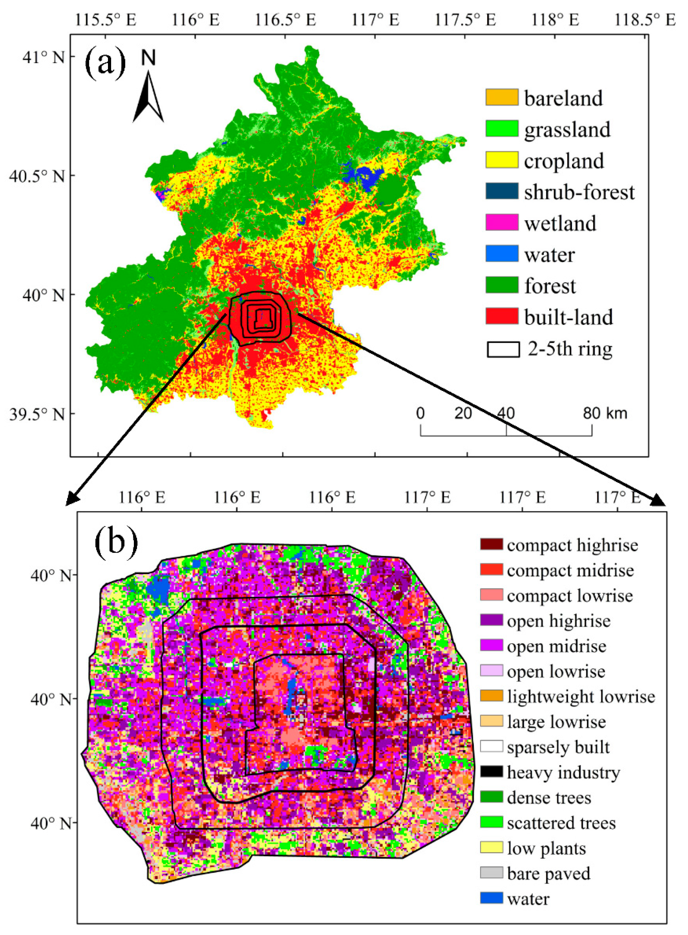
2.1. Study Area

Beijing (39°28′–41°05′N, 115°25′–117°35′E) includes diverse land types and terrains, with an average elevation of approximately 43.5 m. It has a typical continental monsoon climate with an annual mean air temperature of 10–12 °C and mean annual precipitation of 450–550 mm. Herein, study area A is the Beijing city area. It contains four main types of land cover: vegetation, cropland, impervious surfaces (buildings and roads), and water (Figure 1a). The area is about 16,410 km^2, and has a population of about 22 million. Study area B comprises only the 5th ring of Beijing with an area of about 667 km², covered almost entirely by impervious surfaces with relatively flat topography (Figure 1b). The local climate zones of the 5th ring of Beijing are classified by Landsat data, and there is less water and vegetation in the 5th ring. Within the 2nd ring, it is covered mainly by compact midrise and compact lowrise buildings. In the 3rd and 4th rings, there are mainly open buildings. There are more trees and plants in the 4th–5th ring.

2.2. Data

The satellite-based LST data were retrieved from Landsat 8 using the split-window algorithm and data from 22 October 2020 (a sunny and cloud-free day). The overpass time is about 11:30 am in Beijing time. It is mainly sunny in October in Beijing, before and after this date, and the air temperature on this day was within the normal range. The original thermal bands were at 30 m spatial resolution, and LST at 30 m resolution was upscaled to 1080 m, then downscaled to 90 m in this study. LST at 90 m spatial resolution, upscaled from 30 m, was used to validate the downscaled LST. The “upscale-downscale” approach used the same satellite data to validate downscaled LST and avoided errors from different satellite data. The independent variables used in the statistical regression algorithm included spectral reflectance (blue, red, green, near-infrared, short-wave infrared 1, and short-wave infrared 2), spectral indices, building morphology indices, and a DEM (a total of 18 predictors). The spectral indices were calculated from the spectral reflectance of Landsat 8, and building morphology indices were obtained from building vector data. Details of these data and indices are listed in

Table 2. Data used in this study.

Data Type	Data Resource	Spatial Resolution
Land surface temperature	Landsat 8 (http://earthexplorer.usgs.gov/, accessed on 12 October 2021)	30 m
Spectral reflectance	Landsat 8	30 m
DEM	SRTM1 (http://gdex.cr.usgs.gov/gdex/, accessed on 12 October 2021)	30 m
Building boundary and floor numbers	Beijing Institute of Surveying and Mapping	Vector data

and

Table 3. Spectral and building morphology indices used herein for statistical regression.

	Parameter	Full Name	Algorithm
1. Spectral indices	NDVI	Normalized difference vegetation index	$NDVI=\frac{{\rho }_{nir}-{\rho }_{red}}{{\rho }_{nir}+{\rho }_{red}}$ where ρ is band reflectance.
	NDMI	Normalized difference moisture index	$NDMI=\frac{{\rho }_{nir}-{\rho }_{swir2}}{{\rho }_{nir}+{\rho }_{swir2}}$
	NDBI	Normalized difference building index	$NDBI=\frac{{\rho }_{swir2}-{\rho }_{nir}}{{\rho }_{swir2}+{\rho }_{nir}}$
	MNDWI	Modified normalized difference water index	$MNDWI=\frac{{\rho }_{green}-{\rho }_{swir2}}{{\rho }_{green}+{\rho }_{swir2}}$
	NDDI	Normalized difference desert index	$NDDI=\frac{{\rho }_{swir2}-{\rho }_{blue}}{{\rho }_{swir2}+{\rho }_{blue}}$
	NMDI	Normalized multiband drought index	$NMDI=\frac{{\rho }_{nir}-({\rho }_{swir1}-{\rho }_{swir2})}{{\rho }_{nir}+({\rho }_{swir1}-{\rho }_{swir2})}$
2. Building morphology indices	Height	Mean building height	$Height=\frac{{\displaystyle \sum _{i=1}^n{A}_i{H}_i}}{{\displaystyle \sum _{i=1}^n{A}_i}}$ where, Hi is the ith building height, Ai is the plan area of building i, and n is the total number of buildings in one pixel.
	Density	Mean building density	$Density=\frac{{\displaystyle \sum _{i=1}^n{A}_i}}{A_{pixel}}$ where, Ai is the plan area of building i, Apixel is the pixel size, and n is the total number of buildings in one pixel.
	SVF	Sky view factor	$SVF=1-\frac{{\displaystyle \sum _{i=1}^m\sin {\gamma }_i}}{m}$ where, γi is the influence of terrain elevation angle of the ith azimuth angle with unit of radians, m is the number of azimuth angles (m = 36 herein). SVF = 0 means the sky is totally covered. SVF = 1 means the sky is totally open [26].
	λB	Building surface area to plan area ratio	${\lambda }_B=\frac{{\displaystyle \sum _{i=1}^n(A_{r,i}+A_{w,i})}}{A_{pixel}}$ where, Ar,i and Aw,i are the roof area and the area of all walls of building i, respectively.
	FAR	Floor area ratio	$FAR=\frac{{\displaystyle \sum _{i=1}^n{A}_i\times N}}{A_{pixel}}$ where, Ai is the plan area of building i, Apixel is the pixel size, n is the total number of buildings in one pixel, and N is the number of floors of building i.

. In addition, building morphology indices were used only for study area B (5th ring of Beijing) because the building data we obtained does not cover every impervious surface of Beijing.

2.3. Methods

2.3.1. LST Retrieval

A practical split-window algorithm for LST retrieval was proposed by Du et al. (2015) [27], based on radiative transfer theory, as follows:

$$LST=b_0+(b_1+b_2\frac{1-\epsilon }{\epsilon }+b_3\frac{\mathsf{\Delta }\epsilon }{{\epsilon }^2})\frac{T_i+T_j}{2}+(b_4+b_5\frac{1-\epsilon }{\epsilon }+b_6\frac{\mathsf{\Delta }\epsilon }{{\epsilon }^2})\frac{T_i-T_j}{2}+b_7{(T_i-T_j)}^2$$

(1)

where T_i and T_j are the TOA (top of atmosphere) brightness temperature in bands 10 and 11, respectively; ε is the average emissivity of bands 10 and 11; Δε is the emissivity difference (Δε = ε_i − ε_j); and b_k (k = 1, 2, …, 7) are coefficients that can be obtained from the look-up table in Du et al. (2015) [27]. The emissivity algorithm is as follows:

$$\epsilon =P_v{R}_v{\epsilon }_v+(1-P_v)R_m{\epsilon }_m+d_{\epsilon }$$

(2)

$$\left\{\begin{array}{c}{R}_v=0.9332+0.0585P_v\\ R_m=0.9886+0.128P_v\\ R_s=0.9902+0.1068P_v\end{array}\right\}$$

(3)

where P_v is the coverage of vegetation, $P_v={(\frac{NDVI-NDV{I}_s}{NDV{I}_v-NDV{I}_s})}^2$, with NDVIs representing the NDVI values of bare soil or impervious surfaces, and NDVI_v representing the NDVI values of dense vegetation; ε_v, ε_m, and ε_s are the emissivities of vegetation, impervious surfaces, and bare soil, respectively (Equation (2)); and R_v, R_m, and R_s are the LST ratios of vegetation, impervious surfaces, and bare soil, respectively, which can be obtained from P_v (Equation (3)).

2.3.2. Random Forest Method

The RF method was developed based on a decision tree model and is an extension of a bagging algorithm with the advantages of high accuracy, high robustness, and insensitivity to multicollinearity [20,28]. Random forest is an integrated algorithm involving the aggregation of substantial “trees” into a single prediction; each tree is involved in the decision making. A random forest can exploit nonlinear relationships between predictors and dependent variables, and is widely used for regression [5,19,20,28]. Training data are randomly selected by a bootstrap approach, and approximately 37% of samples are not selected when the number of samples is large enough; these are out-of-bag (OOB) samples. The OOB samples can then be used as test data; thus, RF should not deliberately prepare training and test samples. The OOB score is used to judge the performance of the RF model and is indicated as R² (Equations (4)–(6)). Each tree has one R² value, and the average of all the R² values is the OOB score of the RF model. Random forest determines the importance of each predictor by assessing the increase in OOB error when this predictor changes, but other predictors remain constant [29]. OOB error = 1 − R².

This study used OOB samples as test data, and all predictors were input for RF model generation (mtry = all input predictors). The minimum size of terminal nodes “nodesize” = 5. After testing, 500 trees were observed to be sufficient for this study (ntree = 500); the OOB score demonstrated no significant improvement when the number of trees exceeded 500.

$$R^2=1-\frac{u}{v}$$

(4)

$$u={\displaystyle \sum _{i=1}^N{(f_i-y_i)}^2}$$

(5)

$$v={\displaystyle \sum _{i=1}^N{(y_i-\overline{y})}^2}$$

(6)

where R² is the OOB score, u/v is the OOB error, N is the number of samples, f is the simulated value, y is the true value, and $\overline{y}$ is the average of the true values.

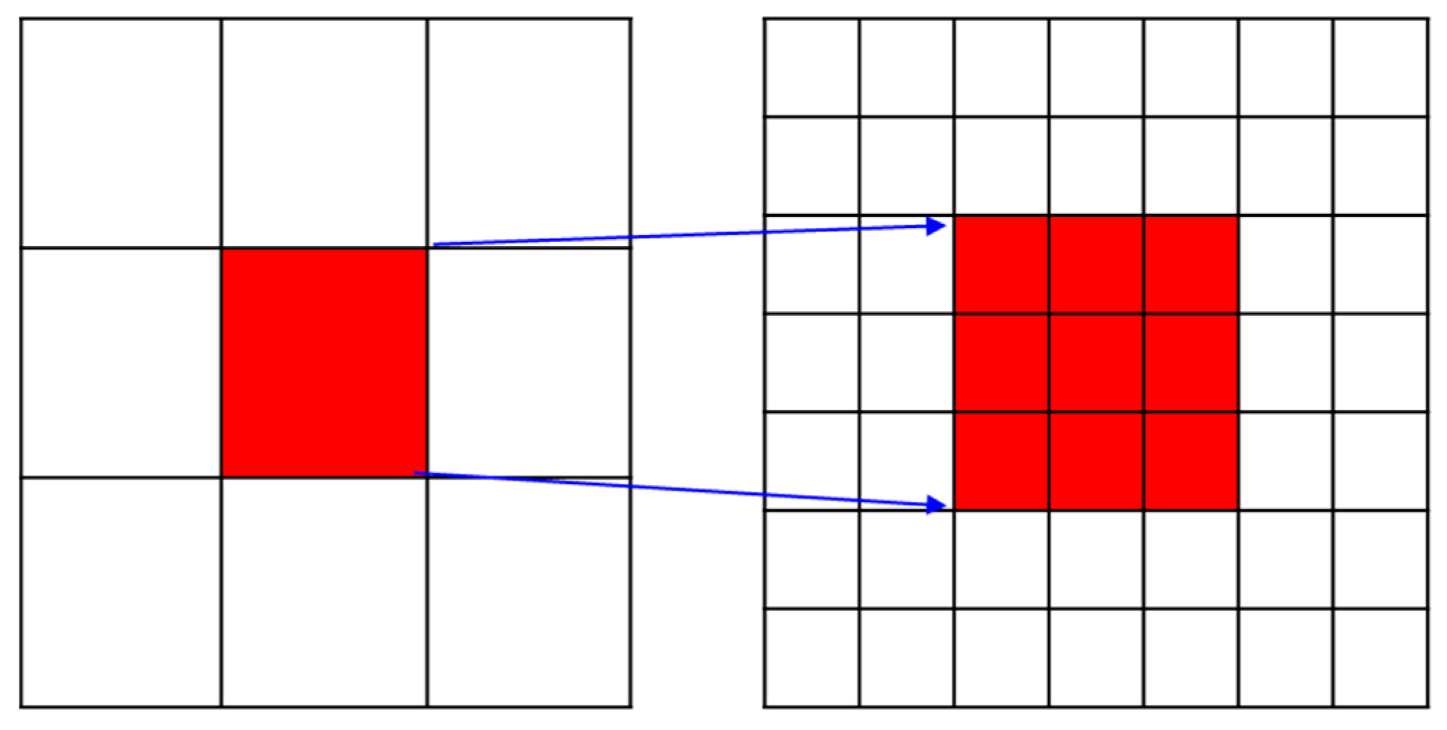
2.3.3. LST Upscaling

This study first upscaled LST, then downscaled it, using Planck’s law to upscale LST from a finer to a coarser resolution, as follows [30]:

$${\epsilon }_c·R(T_c,\lambda )=\frac{{\displaystyle \sum _{i=1}^n{\epsilon }_{i,f}·R(T_{i,f},\lambda )}}{n}$$

(7)

where ε_c and T_c are the land surface emissivity and LST values, respectively, of one pixel at coarser resolution; ε_i,f and T_i,f are the land surface emissivity and LST values, respectively, of pixel i at finer resolution; R() is Planck’s law algorithm; n is the number of pixels at fine resolution that corresponds to the spatial area of the coarse resolution images; ε_c and ε_i,f are calculated using Equation (2).

The Landsat LST at 30 m spatial resolution was upscaled to 90, 540, and 1080 m, respectively.

2.3.4. LST Downscaling

The detailed process of LST downscaling in this study is shown in Figure 2. First, the optimal moving window size was determined using MGWR. Theoretically, MGWR allows different spatial scales for different predictors, showing that the spatial ranges of spatial stationary for each predictor are different. MGWR uses bandwidth to determine the spatial range. Herein, the minimum bandwidth among all bandwidths of predictors was utilized to estimate the optimal moving window size. The window size was approximately equal to the square root of the minimum bandwidth. The minimum bandwidth was chosen because, within the spatial range of the minimum bandwidth, the relationship between predictors and dependent variables is stationary. To obtain a stable bandwidth, we used the Monte Carlo test for spatial variability.

Second, statistical regression using the RF method was executed during the moving window area at coarse resolution, a regression given to the center pixel of the window. Then, regression with finer predictors was used for the spatial area at finer resolution that corresponded to the central pixel area at coarser resolution (red area in Figure 3 left-hand side). Downscaled LST with finer resolution (red area in Figure 3 right-hand side) was thus obtained. The window was moved pixel by pixel.

Third, LST at 1080 m spatial resolution was downscaled with a moving window to 540 m, then to 90 m. The downscaled 540 m LST was corrected by the upscaled 540 m LST. The downscaled 90 m LST was validated by the upscaled 90 m LST.

2.3.5. Metrics

(1)

Pearson correlation coefficient (Pearson’s R)

$$R=\frac{\mathrm{cov}(X,Y)}{{\sigma }_X{\sigma }_Y}$$

(8)

where X is observation, Y is simulation, cov(X,Y) is the covariance of X and Y, σ_X, σ_Y are standard deviations of X and Y.

(2)

Root Mean Square Error (RMSE)

$$RMSE=\sqrt{\frac{{\displaystyle \sum _{i=1}^n{(X-Y)}^2}}{n}}$$

(9)

where X is observation, Y is simulation, n is the number of X or Y,

(3)

Kling Gupta coefficient (KGE)

$$KGE=1-\sqrt{{(1-R)}^2+{(1-\sigma )}^2+{(1-\mu )}^2}$$

(10)

$$\begin{array}{cc}\sigma =\frac{{\sigma }_Y}{{\sigma }_X},& \mu =\frac{{\mu }_Y}{{\mu }_X}\end{array}$$

(11)

where R is the Pearson correlation coefficient, σ_X, σ_Y are standard deviations of X and Y, μ_X and μ_Y are the mean of X and Y.

3. Results and Discussion

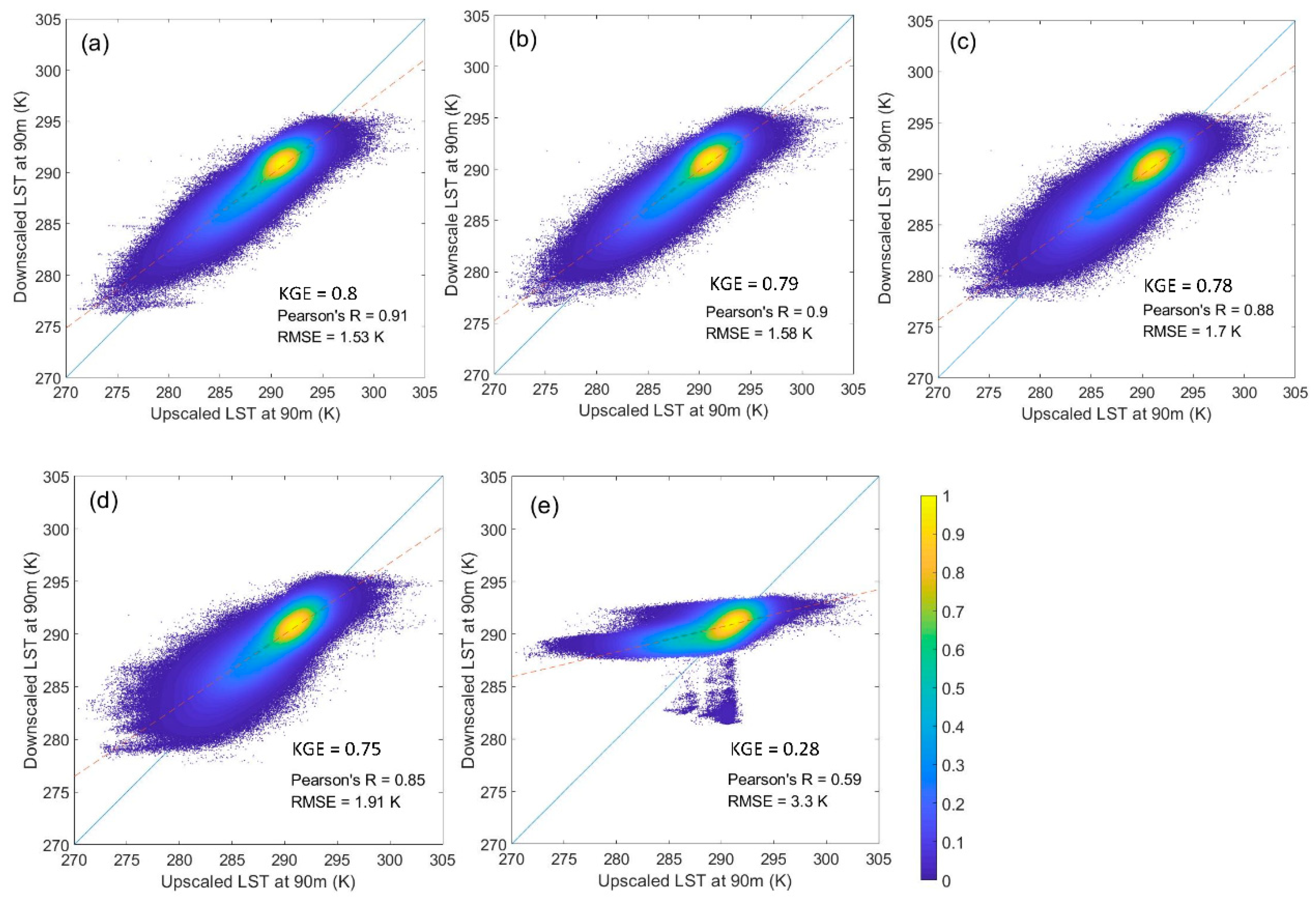
3.1. Comparison of Global and Different Local Windows

The optimal moving window was approximately 7 × 7, estimated using the minimum bandwidth based on MGWR. In addition, downscaled LSTs using other window sizes of 3 × 3, 5 × 5, and 11 × 11 were compared with 7 × 7. Single-step downscaling from 1080 to 90 m was used here, as opposed to the stepwise approach. Figure 4 shows that the downscaled LSTs using different local windows were generally more consistent with observations, with higher Pearson’s correlation coefficients (R) and smaller root-mean-square errors (RMSEs), compared with using the global window. The R and RMSE improved gradually as the window size reduced (e.g., 0.59 and 3.3 K using the global window (Figure 4e) versus 0.91 and 1.53 K using a 3 × 3 window (Figure 4a). Compared to other studies [9,21], RMSE decreased when using a moving window instead of a global window, but RMSE decreased mostly in this study. The KGE are reduced gradually with increasing moving window size and at a minimum with global window (Figure 4). Although the downscaled LSTs using 3 × 3 and 5 × 5 moving windows had higher correlations with observations, their spatial distributions were poor, having fuzzy boundaries of land covers (Figure 5). The number of samples for the regression model was too small with these smaller windows, leading to the generation of unreasonable regression relationships and over-fitting. The downscaled LSTs using 7 × 7 and 11 × 11 windows had clear boundaries of land covers and sharper images (Figure 5c,d). The 7 × 7 window performed better than the 11 × 11 window, with higher r and smaller RMSE (Figure 4c,d).

Theoretically, LST at a finer resolution should show a larger variability because more detailed information is present than at a coarser resolution.

Table 4. Variation range of downscaled LST using different moving windows in study area A.

Window Size	Range (K)	Difference (K)
3 × 3	276–296	20
5 × 5	277–296	19
7 × 7	277–296	19
11 × 11	278–296	18
Global window	281–293	12
LST (1080 m resolution)	278–294	16

shows that the ranges of downscaled LST using local windows were generally larger than LST at 1080 m resolution. However, the downscaled LST using the global window had the smallest range, which shows that the global window does not perform well in revealing LST differences between land covers. The LST difference of 19 K using the 7 × 7 window was a little larger than that using the 11 × 11 window (18 K).

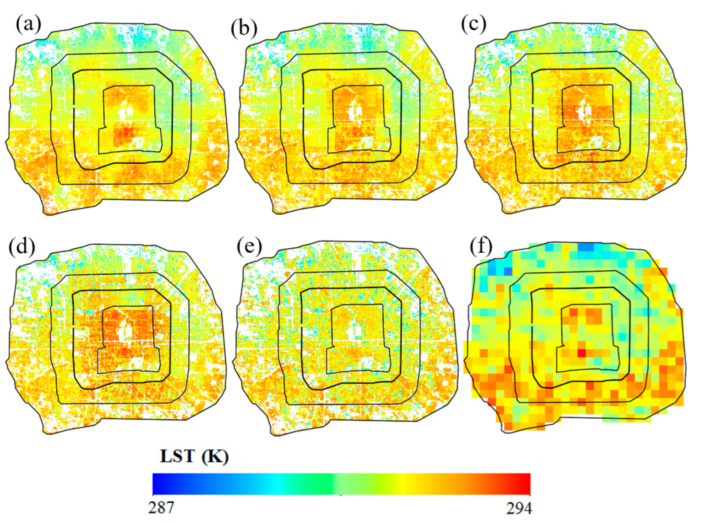
3.2. Stepwise Downscaling of LST

The LSTs downscaled from 1080 to 90 m using the step-by-step and single-step approaches, respectively, were compared with the upscaled LST at 90 m. To highlight the effect of the stepwise approach, the global window, rather than a moving window, was used in this comparison. The step-by-step approach showed improved Pearson’s R (0.68) and RMSE (3.04 K) compared with the single-step approach (r = 0.59; RMSE = 3.3 K) (

Table 5. Downscaling LST from 1080 to 90 m resolution using the global window with step-by-step and single-step approaches, respectively, for Beijing on 22 October 2020.

Downscaling Approach	Pearson’s R	RMSE (K)	KGE
Step-by-step (1080–540–90 m)	0.68	3.04	0.54
Single-step (1080–90 m)	0.59	3.3	0.28

). The KGE was also larger with step-by-step.

The regression relationships between LST and predictors at 1080 m resolution are too crude for use at 90 m and will be missing some detailed information. However, the stepwise downscaling method compensates for this deficiency, to a certain extent, by incorporating 540 m as an intermediate resolution herein.

3.3. Compound Effects of a Local Window and Stepwise Downscaling

LST was downscaled from 1080 to 540 to 90 m by simultaneously using a 7 × 7 local window and a stepwise approach. We also tried adding a further intermediate point at 270 m, between 540 and 90 m, but the result was nearly identical to that from 540 to 90 m and is not displayed here. The Pearson’s R and RMSE using the stepwise approach were 0.89 and 1.72 K, respectively; these were slightly different than the single-step approach (0.88 and 1.70 K, respectively) (

Table 6. Downscaling LST from 1080 to 90 m using a 7 × 7 moving window with step-by-step and single-step approaches, respectively, for Beijing on 22 October 2020.

Downscaling Approach	Pearson’s R	RMSE (K)	KGE
Step-by-step (1080–540–90 m)	0.89	1.72	0.75
Single step (1080–90 m)	0.88	1.7	0.78

). The difference of KGE was also smaller than that with the global window. The advantage of the stepwise approach was diminished when using a local window compared with using the global window. This may be because the purposes of the local window and stepwise approach are both related to obtaining more detailed information for the generation of the regression model.

The 7 × 7 window performed best at 1080 m; however, it may not be the optimal window for other spatial resolutions. Therefore, we used a variable window size during stepwise downscaling. The 7 × 7 window was used from 1080 to 540 m, and 7 × 7, 5 × 5, and 3 × 3 windows were used from 540 to 90 m. The Pearson’s r was 0.89 for all three window sizes, and the RMSEs only varied by a maximum of 0.03 K (

Table 7. Different window combinations for stepwise downscaling in Beijing.

Windows	Pearson’s R	RMSE (K)	KGE
(7 × 7) + (7 × 7)	0.89	1.72	0.75
(7 × 7) + (5 × 5)	0.89	1.71	0.73
(7 × 7) + (3 × 3)	0.89	1.74	0.71

). The KGE with both 7 × 7 window was larger than other windows; however, the KGE difference between the three combinations was not so large (Table 7). It follows that the regression relationships between LST and predictors during the spatial area of 7 × 7 window at 1080 m are stable not only at coarse resolution but also at finer resolutions. The minimal range of spatial stationary obtained by MGWR is suitable for LST downscaling at both coarse and finer resolutions from 1080 to 90 m in this study.

3.4. Downscaling of Impervious Surfaces including Building Morphology

The predictors of building morphology indices were included in study area B, together with spectral reflectance, spectral indices, and a DEM. First, we investigated the impact of different window sizes on LST downscaling. For study area B, the global window performed better than local moving windows (

Table 8. LST in study area B downscaled from 1080 to 90 m using different window sizes, and using building morphology indices, spectral reflectance, spectral indices, and a DEM as predictors.

Windows	Pearson’s R	RMSE (K)	KGE
3 × 3	0.6	1.17	0.28
5 × 5	0.58	1.19	0.25
7 × 7	0.56	1.21	0.39
11 × 11	0.54	1.23	0.39
Global window	0.6	1.16	0.38

), contrary to our findings from study area A. Gao et al., (2017) [4] also showed that the global window performed better over a low heterogeneity area in Beijing, comprising mixtures of urban land and cropland. Long et al., (2021) [31] defined an urban area with a single landcover type as a homogeneous area. Hence, for highly mixed surfaces (e.g., forest, urban, and cropland), a local moving window will perform better than the global window, and it is illogical to perform global regression. However, for impervious surfaces of urban areas, the global window will perform better.

In addition, the spatial distributions of downscaled LST using different windows were essentially consistent with the LST at coarse resolution (Figure 6). However, the window boundary was obvious for the local windows (Figure 6a–d), and LST was regionally continuous for the global window (Figure 6e). In addition, downscaled LST variations reached a maximum when using the global window (

Table 9. Range of downscaled LST recorded using different moving window sizes in study area B.

Windows	Range (K)	Difference (K)
3 × 3	288.4–293.9	5.5
5 × 5	288.5–293.7	5.2
7 × 7	288.4–294	5.6
11 × 11	288.6–294	5.4
Global window	287.6–293.5	5.9
LST at 1080 m	288.8–293.4	4.6

). This shows that some detailed LST information was recovered. We also studied stepwise downscaling for area B, but the results were inferior to the single-step approach and are not displayed herein.

We then compared the downscaled results obtained with and without predictors of building morphology indices (Figure 7). With the inclusion of building morphology indices, LST downscaling improved slightly; RMSE improved by 0.01 K, and Pearson’s R improved by 0.01. This may be because the impact of building morphology on LST at a scale of 1080 m is not significant. The relationship between LST and predictors simulated at 1080 m was applied at 90 m, so the impact of building morphology is also not significant at 90 m. It may also be because only the predictors in the overlap area of all predictors (the building footprint area) are used for the generation of the regression relationship, which is too limited.

Compared with the upscaled 90 m LST, the LST downscaled from 1080 m using the RF model that included building morphology was not improved significantly (Figure 7). However, the ability of the RF model to perform regression was improved when including building morphology, especially at the 90 m scale (Table 9). This shows that building morphology impacts LST, and it also has a scaling effect. In Figure 7, the simulated relationship between LST and predictors at 1080 m is applied to 90 m for downscaling. In addition, morphology is less important than spectral factors at 1080 m, thus, the impact of morphology at 90 m is not revealed well. It may also be because there was no other urban morphology (e.g., trees) included in this study; only data from areas covered with buildings were used, and the number of samples for regression was limited. In the future, thermal airborne high spatial resolution data will be an important dataset for studying the impact of urban morphology on LST at very high spatial resolutions (e.g., 20–30 m).

3.5. Scaling Effect of Building Morphology

The OOB scores of the RF model that included building morphology indices were generally improved at both the 1080 and 90 m scales (

Table 10. The OOB scores of the RF model with different predictors at different spatial scales in study area B.

Predictors	1080 m	90 m
Spectral reflectance, spectral indices, and DEM	0.44	0.35
Spectral reflectance, spectral indices, DEM, and building morphology indices	0.46	0.46

); the improvement was greater at 90 m (0.35 to 0.46) than at 1080 m (0.44 to 0.46). This shows that the performance of the RF model for regression is improved by including building morphology. Furthermore, building morphology has a greater impact on LST at a finer scale.

The relative importance of predictors at scales of 1080 and 90 m, respectively, is shown in Figure 8. Although spectral factors have greater importance than building morphology at 1080 m, building height becomes the second largest factor (behind only red reflectance) at 90 m. In addition, the importance of SVF, building height, and density at 90 m is greater than at 1080 m.

4. Conclusions

In this study, a general goal was to improve the accuracy of LST downscaling using the random forest model. We investigated two approaches: local downscaling with a moving window; and stepwise downscaling of spatial resolution. We then discussed the impact and scaling effect of building morphology on LST.

Multi-scale geographically weighted regression was used to find the optimal moving window based on the bandwidth of each predictor. The LST retrieved from Landsat 8 was upscaled to 1080 m, then downscaled to 90 m, and validated by the upscaled 90 m LST. For stepwise downscaling, the coarse 1080 m resolution LST was downscaled to 540 then 90 m. The main findings of this study are as follows:

(1) The performances of local and stepwise LST downscaling are dependent on the extent of surface heterogeneity. For study area A, with mixed surfaces of forest, cropland, and urban, local downscaling using different sizes of moving windows (3 × 3, 5 × 5, 7 × 7, and 11 × 11) generally performed better than using the global window. Pearson’s R increased from 0.59 to 0.91. RMSE decreased from 3.3 to 1.53 K. Stepwise downscaling from 1080 to 540 to 90 m also performed better than direct downscaling from 1080 to 90 m, with Pearson’s R improving from 0.59 to 0.68 and RMSE from 3.3 to 3.0 K. However, for study area B (urban cover only), the global window performed better than a local moving window, with a higher Pearson’s R and lower RMSE. The stepwise approach was weakened when combined with the moving window approach for downscaling in study area A.

As far as global window, moving window, stepwise, or single step, which pair combination is best for LST downscaling? According to the above mentioned, for a high heterogeneity area (study area A), moving window + stepwise or moving window + single step is best. For a low heterogeneity area (study area B), global window + single step is good.

(2) The MGWR method was found to be a feasible approach for identifying the optimal window for LST downscaling based on the bandwidth of each predictor. In this study, a 7 × 7 window was determined to be the optimal moving window. Although the downscaled LSTs using 3 × 3 and 5 × 5 windows showed higher correlations with observations from study area A, the spatial distributions were poor, with fuzzy boundaries between different land covers. The 7 × 7 window performed better than the 11 × 11 window, with a higher Pearson’s R and smaller RMSE. Furthermore, a variable window size was applied during stepwise downscaling in study area A; a 7 × 7 window was used from 1080 to 540 m, and 3 × 3, 5 × 5, and 7 × 7 windows were used from 540 to 90 m. However, the results obtained using variable window sizes were near-identical to those obtained using a fixed window size, having the same Pearson’s R and a maximum RMSE change of only 0.03. This further illustrates that the optimal window obtained using the MGWR method is suitable for LST downscaling at both coarse and finer spatial resolutions.

(3) Building morphology has an impact and scaling effect on urban LST; it has more impact on LST at a finer scale. Although the Pearson’s R was only increased by 0.01 and RMSE reduced by 0.01 K when including predictors of building morphology indices in study area B, the performance of the RF model for regression was improved. The OOB score of the RF model increased from 0.44 to 0.46 at 1080 m, and from 0.35 to 0.46 at 90 m, when predictors of building morphology indices were included. In addition, the importance of SVF, building height, and density at 90 m resolution was greater than at 1080 m.

Strictly speaking, the relationships between LST and predictors over heterogeneous surfaces are variable across different scales. However, most LST downscaling studies assume these relationships are scale-invariant. The findings of this study show that the impacts of building morphology on LST are different at 1080 and 90 m spatial resolutions over an urban area. Although in this study we used the same relationships at both 1080 m and 90 m, it may not be suitable for higher spatial resolution. Pu (2021) [32] showed the relationship between LST and predictors at spatial resolution beyond a range (20~30 m) is relatively steady; however, within this range, this relationship is no longer applicable. Hence, ways to generate a scale-adaptive relationship, and further study the impact of urban morphology on LST, are important issues that need to be resolved in future studies.

References

1. Duan, S.; Chen, R.; Zhaoliang, L.; Mengmeng, W.; Hanqiu, X.; Hua, L.; Penghai, W.; Wenfeng, Z.; Ji, Z.; Wei, Z.; et al. Reviews of methods for land surface temperature retrieval from Landsat thermal infrared data. Natl. Remote Sens. Bull. 2021, 25, 1591–1617. [Google Scholar] [CrossRef]
2. Li, N.; Wu, H.; Luan, Q. Land surface temperature downscaling in urban area: A case study of Beijing. Natl. Remote Sens. Bull. 2021, 25, 1808–1820. [Google Scholar] [CrossRef]
3. Wu, H.; Li, X.; Li, Z.; Duan, S.; Qian, Y. Hyperspectral thermal infrared remote sensing: Current status and perspectives. Natl. Remote Sens. Bull. 2021, 25, 1567–1590. [Google Scholar] [CrossRef]
4. Gao, L.; Zhan, W.; Huang, F.; Quan, J.; Lu, X.; Wang, F.; Ju, W.; Zhou, J. Localization or Globalization? Determination of the Optimal Regression Window for Disaggregation of Land Surface Temperature. IEEE Trans. Geosci. Remote Sens. 2017, 55, 477–490. [Google Scholar] [CrossRef]
5. Li, W.; Ni, L.; Li, Z.L.; Duan, S.B.; Wu, H. Evaluation of Machine Learning Algorithms in Spatial Downscaling of MODIS Land Surface Temperature. IEEE J. Sel. Top. Appl. Earth Obs. Remote Sens. 2019, 12, 2299–2307. [Google Scholar] [CrossRef]
6. Dominguez, A.; Kleissl, J.; Luvall, J.C.; Rickman, D.L. High-resolution urban thermal sharpener (HUTS). Remote Sens. Environ. 2011, 115, 1772–1780. [Google Scholar] [CrossRef] [Green Version]
7. Zakšek, K.; Oštir, K. Downscaling land surface temperature for urban heat island diurnal cycle analysis. Remote Sens. Environ. 2012, 117, 114–124. [Google Scholar] [CrossRef]
8. Agam, N.; Kustas, W.P.; Anderson, M.C.; Li, F.; Neale, C.M.U. A vegetation index based technique for spatial sharpening of thermal imagery. Remote Sens. Environ. 2007, 107, 545–558. [Google Scholar] [CrossRef]
9. Duan, S.-B.; Li, Z.-L. Spatial Downscaling of MODIS Land Surface Temperatures Using Geographically Weighted Regression: Case Study in Northern China. IEEE Trans. Geosci. Remote Sens. 2016, 54, 6458–6469. [Google Scholar] [CrossRef]
10. Gao, F.; Masek, J.; Schwaller, M.; Hall, F. On the blending of the Landsat and MODIS surface reflectance: Predicting daily Landsat surface reflectance. IEEE Trans. Geosci. Remote Sens. 2006, 44, 2207–2218. [Google Scholar] [CrossRef]
11. Zhu, X.; Chen, J.; Gao, F.; Chen, X.; Masek, J.G. An enhanced spatial and temporal adaptive reflectance fusion model for complex heterogeneous regions. Remote Sens. Environ. 2010, 114, 2610–2623. [Google Scholar] [CrossRef]
12. Weng, Q.; Fu, P.; Gao, F. Generating daily land surface temperature at Landsat resolution by fusing Landsat and MODIS data. Remote Sens. Environ. 2014, 145, 55–67. [Google Scholar] [CrossRef]
13. Yin, Z.; Wu, P.; Foody, G.M.; Wu, Y.; Liu, Z.; Du, Y.; Ling, F. Spatiotemporal Fusion of Land Surface Temperature Based on a Convolutional Neural Network. IEEE Trans. Geosci. Remote Sens. 2021, 59, 1808–1822. [Google Scholar] [CrossRef]
14. Guo, L.J.; Moore, J.M. Pixel block intensity modulation: Adding spatial detail to TM band 6 thermal imagery. Int. J. Remote Sens. 1998, 19, 2477–2491. [Google Scholar] [CrossRef]
15. Norman, J.M.; Anderson, M.C.; Kustas, W.P.; French, A.N.; Mecikalski, J.; Torn, R.; Diak, G.R.; Schmugge, T.J.; Tanner, B.C.W. Remote sensing of surface energy fluxes at 101-m pixel resolutions. Water Resour. Res. 2003, 39, 1221. [Google Scholar] [CrossRef] [Green Version]
16. Merlin, O.; Al Bitar, A.; Walker, J.P.; Kerr, Y. An improved algorithm for disaggregating microwave-derived soil moisture based on red, near-infrared and thermal-infrared data. Remote Sens. Environ. 2010, 114, 2305–2316. [Google Scholar] [CrossRef] [Green Version]
17. Mpelasoka, F.S.; Mullan, A.B.; Heerdegen, R.G. New Zealand climate change information derived by multivariate statistical and artificial neural networks approaches. Int. J. Climatol. 2001, 21, 1415–1433. [Google Scholar] [CrossRef]
18. Gualtieri, J.A.; Chettri, S. Support vector machines for classification of hyperspectral data. In Proceedings of the IGARSS 2000, IEEE 2000 International Geoscience and Remote Sensing Symposium, Taking the Pulse of the Planet: The Role of Remote Sensing in Managing the Environment, Proceedings (Cat. No.00CH37120), Honolulu, HI, USA, 24–28 July 2000; Volume 812, pp. 813–815. [Google Scholar]
19. Hutengs, C.; Vohland, M. Downscaling land surface temperatures at regional scales with random forest regression. Remote Sens. Environ. 2016, 178, 127–141. [Google Scholar] [CrossRef]
20. Yang, Y.; Cao, C.; Pan, X.; Li, X.; Zhu, X. Downscaling Land Surface Temperature in an Arid Area by Using Multiple Remote Sensing Indices with Random Forest Regression. Remote Sens. 2017, 9, 789. [Google Scholar] [CrossRef] [Green Version]
21. Yang, Y.; Li, X.; Cao, C. Downscaling urban land surface temperature based on multi-scale factor. Sci. Surv. Mapp. 2017, 42, 73–79. [Google Scholar] [CrossRef]
22. Zhu, X.; Song, X.; Leng, P.; Hu, R. Spatial downscaling of land surface temperature with the multi-scale geographically weighted regression. Natl. Remote Sens. Bull. 2021, 25, 1749–1766. [Google Scholar] [CrossRef]
23. Yu, H.; Fotheringham, A.S.; Li, Z.; Oshan, T.; Kang, W.; Wolf, L.J. Inference in Multiscale Geographically Weighted Regression. Geogr. Anal. 2020, 52, 87–106. [Google Scholar] [CrossRef]
24. Fotheringham, A.S.; Yang, W.; Kang, W. Multiscale Geographically Weighted Regression (MGWR). Ann. Am. Assoc. Geogr. 2017, 107, 1247–1265. [Google Scholar] [CrossRef]
25. Li, N.; Yang, J.; Qiao, Z.; Wang, Y.; Miao, S. Urban Thermal Characteristics of Local Climate Zones and Their Mitigation Measures across Cities in Different Climate Zones of China. Remote Sens. 2021, 13, 1468. [Google Scholar] [CrossRef]
26. Liang, C.; Ng, E.; An, X.; Chao, R.; Lee, M.; Wang, U.; He, Z. Sky view factor analysis of street canyons and its implications for daytime intra-urban air temperature differentials in high-rise, high-density urban areas of Hong Kong: A GIS-based simulation approach. Int. J. Climatol. 2012, 32, 121–136. [Google Scholar] [CrossRef]
27. Du, C.; Ren, H.; Qin, Q.; Meng, J.; Zhao, S. A Practical Split-Window Algorithm for Estimating Land Surface Temperature from Landsat 8 Data. Remote Sens. 2015, 7, 647. [Google Scholar] [CrossRef] [Green Version]
28. Breiman, L. Random Forests. Mach. Learn. 2001, 45, 5–32. [Google Scholar] [CrossRef] [Green Version]
29. Genuer, R.; Poggi, J.-M.; Tuleau-Malot, C. Variable selection using random forests. Pattern Recognit. Lett. 2010, 31, 2225–2236. [Google Scholar] [CrossRef] [Green Version]
30. Zhu, J.; Zhu, S.; Yu, F.; Zhang, G.; Xu, Y. A downscaling method for ERA5 reanalysis land surface temperature over urban and mountain areas. Natl. Remote Sens. Bull. 2021, 25, 1778–1791. [Google Scholar] [CrossRef]
31. Long, L.; Li, J.; Chen, Y.; Xia, H.; Chen, Q. An Auto-Adjusted Kernel Method for Thermal Sharpening with Local and Object-Based Window Strategies. IEEE J. Sel. Top. Appl. Earth Obs. Remote Sens. 2021, 14, 3659–3668. [Google Scholar] [CrossRef]
32. Pu, R.L. Assessing scaling effect in downscaling land surface temperature in a heterogenous urban environment. Int. J. Appl. Earth Obs. Geoinf. 2021, 96, 102256. [Google Scholar] [CrossRef]
Figure 1. Study areas (a,b) with land cover types. Landcover types in area (a) in 2020 are from the GlobalLand30 product; the local climate zones of area (b) are classified using Landsat 8 imagery [25].
Remotesensing 14 02390 g001
Figure 2. Flowchart of the local LST downscaling procedure using the RF method; subscript “f” represents finer resolution, and subscript “c” represents coarser resolution.
Remotesensing 14 02390 g002
Figure 3. Simple schematic diagram of a downscaled area using a moving window; left is the window at coarser resolution, right is the window at finer resolution; red area on the right is the downscaled area.
Remotesensing 14 02390 g003
Figure 4. Density scatter plots of the downscaled and upscaled LST at 90 m resolution in Beijing on 22 October 2020, using different moving window sizes. Window sizes: (a) 3 × 3; (b) 5 × 5; (c) 7 × 7; (d) 11 × 11; and (e) global window.
Remotesensing 14 02390 g004
Figure 5. Spatial distributions of LST downscaled from 1080 to 90 m, using moving windows of: (a) 3 × 3; (b) 5 × 5; (c) 7 × 7; (d) 11 × 11; (e) global window; and (f) the 90 m LST retrieved by Landsat 8, in Beijing on 22 October 2020.
Remotesensing 14 02390 g005
Figure 6. Spatial distribution of LST downscaled directly from 1080 to 90 m with a single step, using windows of: (a) 3 × 3; (b) 5 × 5; (c) 7 × 7; (d) 11 × 11; (e) global; and (f) coarse-scale LST at 1080 m resolution.
Remotesensing 14 02390 g006
Figure 7. Density scatter plots of upscaled 90 m LST versus LST downscaled from 1080 to 90 m using a single step and global window. (a) Using predictors of spectral reflectance, spectral indices, and DEM. (b) Using predictors in (a) plus building morphology indices.
Remotesensing 14 02390 g007
Figure 8. Relative importance of different predictors at scales of (a) 1080 m and (b) 90 m in study area B.
Remotesensing 14 02390 g008