Article

Monitoring Sand Spit Variability Using Sentinel-2 and Google Earth Engine in a Mediterranean Estuary

1
Instituto de Ciencias Marinas de Andalucía (ICMAN-CSIC), Campus Universitario Río San Pedro, s/n, Puerto Real, E-11510 Cadiz, Spain
2
Facultad de Ciencias del Mar y Ambientales (CASEM), Campus Universitario Río San Pedro, s/n, Puerto Real, E-11510 Cadiz, Spain
*
Author to whom correspondence should be addressed.
Remote Sens. 2022, 14(10), 2345; https://doi.org/10.3390/rs14102345
Submission received: 12 April 2022 / Revised: 5 May 2022 / Accepted: 11 May 2022 / Published: 12 May 2022
(This article belongs to the Special Issue Advances in Remote Sensing of the Inland and Coastal Water Zones)

Abstract

:
Estuarine degradation is a major concern worldwide, and is rapidly increasing due to anthropogenic pressures. The Mediterranean Guadiaro estuary, located in San Roque (Cadiz, Spain), is an example of a highly modified estuary, showing severe negative effects of eutrophication episodes and beach erosion. The migration of its river mouth sand spit causes the closure of the estuary, resulting in serious water quality issues and flora and fauna mortality due to the lack of water renewal. With the aim of studying the Guadiaro estuary throughout a 4-year period (2017–2020), the Sentinel-2 A/B twin satellites of the Copernicus programme were used thanks to their 5-day and 10 m temporal and spatial resolution, respectively. Sea–land mapping was performed using the Normalized Difference Water Index (NDWI) in the Google Earth Engine (GEE) platform, selecting cloud-free Sentinel-2 Level 2A images and computing statistics. Results show a closure trend of the Guadiaro river mouth and no clear sand spit seasonal patterns. The study also reveals the potential of both Sentinel-2 and GEE for estuarine monitoring by means of an optimized processing workflow. This improvement will be useful for coastal management to ensure a continuous and detailed monitoring in the area, contributing to the development of early-warning tools, which can be helpful for supporting an ecosystem-based approach to coastal areas.

1. Introduction

Estuarine eutrophication is one of the most common and harmful environmental problems in coastal areas around the globe [1]. The world has lost 50% of its natural wetlands since 1900, most of them located in highly anthropized areas of the temperate zone in the northern hemisphere [2]. Anthropogenic pressure is the main vector for estuarine ecosystem alteration, accelerating the deterioration of water quality in natural coastal wetlands. Littoral population settlements have greatly increased in the last decades, gathering more than 30% of the world population [3] and expanding faster than any other region [4]. This ongoing trend of coastal migration extends especially to flat estuarine lands, linked to urbanization processes and human activities [5]. Across the Western Mediterranean, both climate change and anthropic activities have had impacts on water quality across coastal areas. Some examples, commonly associated to river discharges, are the Mar Menor cyclic environmental collapse [6] and the permanent eutrophication in the Albufera of Valencia [7]. To mitigate anthropic impacts, adaptive policies are needed [8], and consequently, monitoring is also required, this information being crucial for optimized coastal wetland management.
Estuary systems evolve very rapidly with channel migrations, loss of sand and erosion/accretion of adjacent beaches [9]. This study is focused on the Guadiaro estuary, located in San Roque, Cádiz (Spain), which delta started to disappear during the 1970s, as seen in Figure 1, caused by multiple factors but massive extraction of sediments along the basin was decisively, consequently reducing the sedimentary input in the Guadiaro system [10]. As a complex enclave, the Guadiaro estuary has been widely studied by engineers and scientists in the last 20 years in order to characterize and effectively manage the area [9,10,11,12], albeit without using a continuous monitoring technique.
In order to manage this ecosystem, it is important to understand and evaluate the sand spit patterns, where information and knowledge are essential. Therefore, improved monitoring to evaluate the different scenarios is required [13], in particular, to determine spatio-temporal variability of the sand spit closing. The context affecting the Guadiaro estuary and its surrounding requires an efficient and real-time method of monitoring the state of the sand spit. Traditional monitoring approaches are labor intensive and time consuming when long-term monitoring and management are required, and new technologies can play a powerful part. Furthermore, integrated coastal management requires information during the entire management cycle [14,15,16,17]. In practice, a monitoring tool developed with the proper technology should be able to provide long-term sustained information, required for an adaptive ecosystem-based management approach [18,19,20]. This means the monitoring tool can be used not only as an early-warning system, but also to evaluate responses given by the administration correlated to changes of state [21].
Earth Observation (EO) tools and remote-sensing techniques yield precise data thanks to the wide range of sensors and their spatio-temporal resolution. Satellite imagery is especially useful for shoreline and coastal monitoring [22,23,24,25], with increased public availability through open access programs. The European Copernicus programme is the EO program of the European Commission and the European Space Agency (ESA). It is composed of a set of dedicated satellites called “Sentinel” under an open and free policy. Sentinel-2A/B (S2) satellites are part of this Sentinel family, with images of 10–20–60 m and 5-day spatial and temporal resolutions, respectively, are very useful for studying coastal processes [26,27,28,29]. These satellites carry the MultiSpectral Instrument (MSI) sensor whose bands are useful for sea–land mapping. To process this huge amount of data, costly high-computational capacity and long-processing times are required [30]. Nevertheless, imagery data production has been improved in parallel to software development, which enables powerful geoprocesses resulting in more accessible and faster analysis.
The use of satellite imagery also has of the advantage of using available open-source tools for image processing, such as Google Earth Engine (GEE). GEE is a free cloud-based platform for planetary-scale geospatial analysis [31] which has a massive catalogue of satellite imagery and geospatial datasets available. This platform allows this information to be processed in the cloud in order to detect changes, map trends and quantify differences on the Earth’s surface, and can develop applications for final users [32]. Some studies have been carried out using S2 and GEE platform in marine and coastal areas, including water quality studies [33,34], coastline evolution [35,36], coastal management [37], and wetland mapping [38], showing the potential of the Copernicus open data and the GEE open-source platform for coastal monitoring.
An integrated sea–land approach is needed to quantify coastal changes [39]. Some studies carried out this approach manually [40], which is more precise but time consuming and non-viable for monitoring tools, which need more automatic workflows [22]. Sea–land mapping is mostly used for coastline evolution studies, including erosion and accretion trends or sea-level rise [23,41,42], using image classification, image segmentation, and several indices. However, the use of indices based on optical properties has proven its optimized performance against image classification and segmentation methods in order to detect water and non-water pixels [43,44]. Among the different indices, the Normalized Difference Water Index (NDWI), defined by McFeeters, is widely accepted for this purpose [45], as well as the Modified NDWI (MNDWI) [45,46,47,48], although other indices have been developed, such as the AWEI index [49] or the MuWi index [50]. According to Rokni et al., the MNDWI index has been generally developed for application in urbanized areas [51], whereas the NDWI is better used in natural coasts [44].
This study evaluates the use of S2-A/B satellites for sea–land mapping in the Guadiaro estuary using the NDWI and GEE between 2017 and 2020. Using the innovative GEE platform, we explore the suitability of the S2 Level-2 A (L2A) dataset for multi-temporal studies and developed a JavaScript algorithm generating an operational monitoring tool. S2 images can serve as an input for continuous and low-cost monitoring information with GEE, which can be complemented with in situ sampling. This information would be useful for stakeholders and coastal managers in order to address the persistent problems in the Guadiaro river. The monitoring tool would help as an evaluation method for adapting management actions throughout the cycle, as an early-warning system for eutrophication episodes and as a pilot to be used in other estuaries. Therefore, this tool can be implemented not only operationally, but also as a valuable information system for strategic and adaptive coastal management. The aim is to contribute to coastal management by means of developing and evaluating a methodology in GEE for monitoring the sand spit spatio-temporal patterns as a pilot project.

2. Materials and Methods
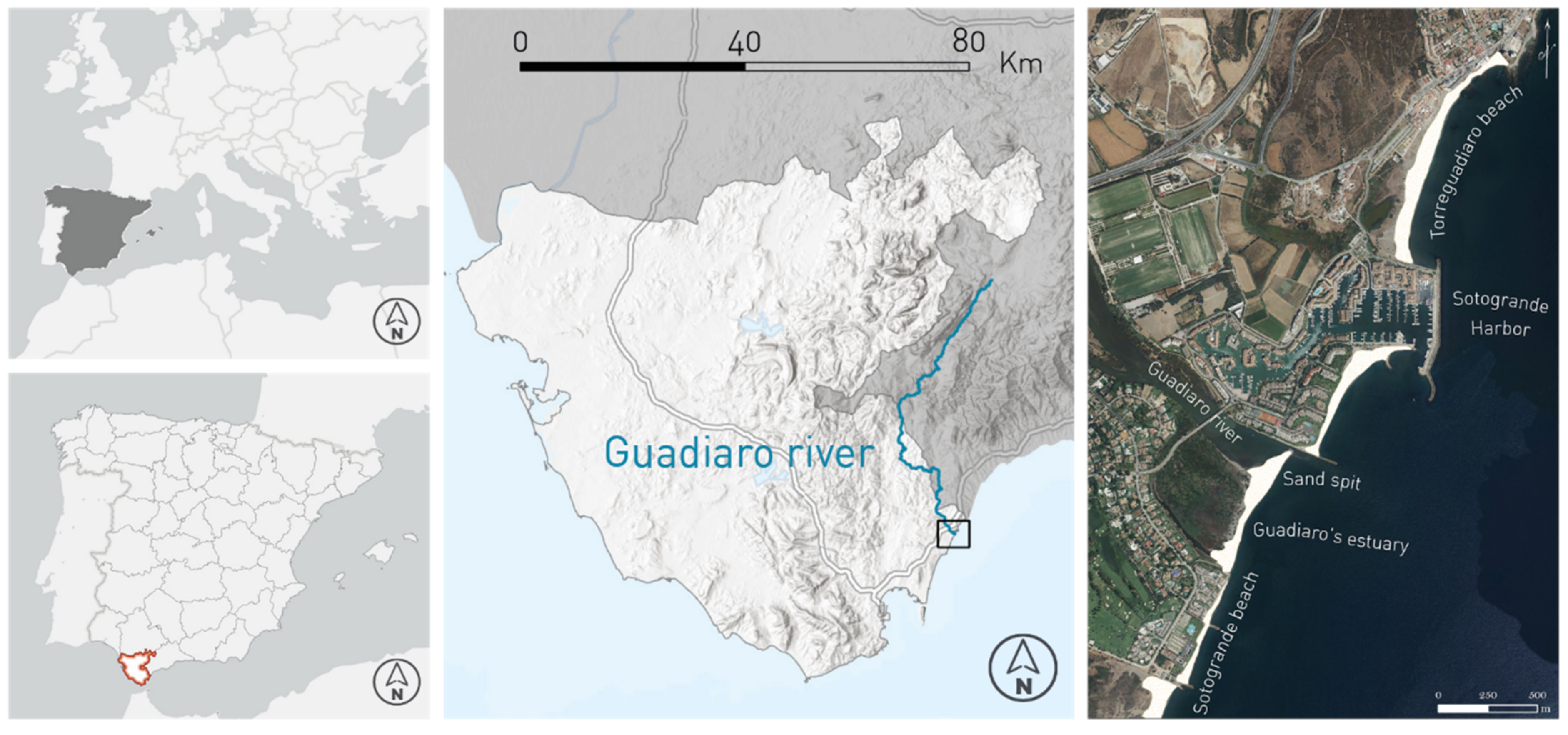
2.1. Study Area

The Guadiaro estuary is a semi-closed Mediterranean coastal lagoon located in the Strait of Gibraltar, San Roque (Cadiz, southern Spain) (Figure 2), the only coastal wetland along 115 km of coastline [10]. This estuary is a multi-use water resource system, including fish nurseries, flood control and recreational and cultural services. Due to the micro-tidal conditions of about 40 cm, shallow bathymetry, severe wave refraction [9], and sediment transportation following the main longitudinal current right to the Strait of Gibraltar with a SW component [52]. Regarding the meteorology, the Guadiaro river is characterized by its irregular and strong dependence on rainfall regime and torrential character [11,53,54], the sand spit behavior being strongly dependent on the river, and by the sea being dependent on E winds and consequent wave behavior [11]. On the other hand, Sotogrande beach suffers from chronical erosion trends, having a regression by more than 160 m which was evident between 1960 and 2000, and is still going (−3.1 m/year) [55]. This implies an increase in vulnerability to climate change due to forecasts of increased wave energy [9,10,11,56].
Throughout recent decades, the Guadiaro estuary has experienced several problems, suffering from eutrophication episodes with harmful consequences for the biota and direct impacts on tourism. Its major concern is that the Guadiaro river mouth is frequently partially or totally closed by its sand spit formation. This occurs partly due to the presence of a local coastal drift current inverse to the predominant one [10,53], which transports sediment northwards and blocks water renewal in the estuary. Furthermore, during the summer, waves tend to close the Guadiaro river mouth as a result of the weak current, reducing the water renewal rate with the consequent reduction in oxygen levels and increased eutrophication [57]. Anthropogenic discharges as well as uncontrolled tourism further aggravate the problem [9]. In only 3 years (2016–2018) the Spanish Government invested more than EUR 0.5 M on dredging the Guadiaro river mouth, retrieving almost 85,000 m3 of sand used mainly to support the Sotogrande beach, which suffers from a severe erosive trend. In extreme eutrophication episodes, the Guadiaro estuary urges from artificial sand spit openings, which are very expensive, as can be seen in Figure 3. This fact reflects the need to develop a more complete coastal management strategy for its optimization, including monitoring tools, operational early-warning systems, as well as the improvement of coordination and cooperation processes.
Considering the different activities developed in the Guadiaro river and the littoral zone, both river and coastal processes have been highly modified since the 1970s. The Port of Sotogrande was built in 1987 to the north of to the river mouth. Two groins were built in 1973 (one removed 2 years later) and the port breakwater was constructed in 1986 and extended by 1994 [12]. Due to sand extraction activities, with 8 mining concessions by 2009, the river sediment input decreased from 100,000 m3/year in the 1960s to 50,000 m3/year in 2009 [14]. Furthermore, an inter-basin upstream transfer was carried out in the upper course of the Guadiaro river to the Majaceite River in 1999, with a maximum transfer capacity of 30,000 m3/year [58], altering the sedimentary balance, decreasing river flow strength, and reducing mouth flow peaks and, consequently, favoring river mouth closure [12]. Moreover, considering other factors, such us agricultural and urban waste, extraction of water for agricultural use and the Sotogrande urbanization, the Guadiaro estuary experiences periodic biota mortality episodes with massive fish kills directly related with the sand spit closing and lack of oxygen availability [10].

2.2. Satellite Data

The Guadiaro estuary covers a local area with a high morpho-dynamic variability, requiring high spatial resolution and short-term revisit time, for which S2-A/B satellites have been used. S2 L2A refers to the level in which images are categorized in the MSI S2 database on-board S2. In GEE, two levels are currently available: Level 1 (“COPERNICUS/S2”) and Level 2A (“COPERNICUS/S2_SR”). Level 1-C (L1C) contains images radiometrically and geometrically corrected at Top Of Atmosphere (TOA) reflectance, while L2A contains orthorectified atmospherically corrected surface reflectance, being a Bottom Of Atmosphere (BOA) product. Therefore, L2A datasets have been selected with the atmospheric correction applied, which determines a faster geo-processing workflow and improved enforcement of normalized indices. However, almost two years of data cannot be used for the study, with L1C available from 23 June 2015 to present and S2 L2A images from 30 March 2017 to present, which explains the lack of data in winter 2017 in the following results.

2.3. GEE & GIS

The GEE platform was used to process S2 images for its high computational and on-the-cloud capacity, having a wide variety of datasets available without depending on download. As atmospheric correction remains a challenge, we used atmospheric corrected S2 L2A images (corresponding to “COPERNICUS/S2_SR” in GEE). Using these images, we developed a workflow in JavaScript Code Editor interface in GEE in four main steps, as shown in Figure 4. (1) cloud coverage image selection in the Area Of Interest (AOI); (2) band computing according to NDWI index; (3) statistics calculation including climatology and Variation Rate (VR); (4) export results to Google Drive. As a final step, design was developed using ArcGIS Pro.

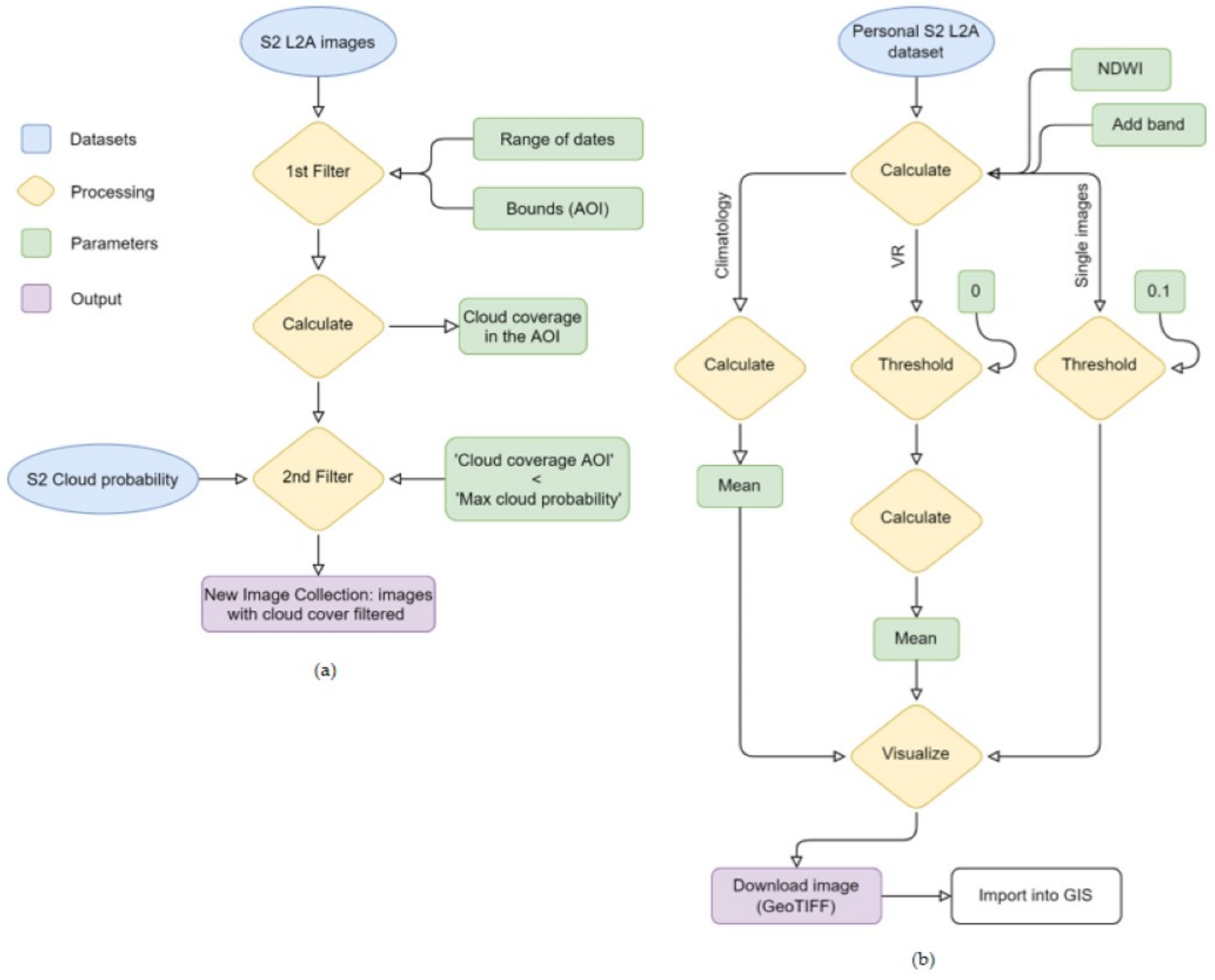
2.3.1. Cloud Coverage

Clouds are one of the main challenges faced by optical sensors on-board satellites in order to obtain useful data. The presence of clouds and cloud shadows in images introduces noise to data, which may result in these data being masked out. Therefore, pre-processing for cloud-free image selection has to be performed before processing any algorithm in order to obtain reliable results. In this step, we implemented a workflow developed in GEE through which cloud cover is calculated in the study area (AOI) and images can be filtered in a maximum cloud cover custom percentage from the original dataset (“COPERNICUS/S2_SR”).
The geoprocessing workflow, showed in Figure 4a and available in GEE (https://code.earthengine.google.com/6363973f5918f3eacd09d890a52f5827, accessed on 1 February 2021) involved clipping the AOI from the S2 L2A image collection and filtering it by date from the first image available (30 March 2017) to December 2020. After this, cloud mask property, a general variable pre-calculated for the whole tile, was used from the S2 L2A metadata to calculate the cloud coverage in the specific AOI. With these data, the cloud cover percentage was obtained in the AOI for each image, representing valuable information for a second filtering. Finally, with the S2 Cloud probability dataset (“COPERNICUS/S2_CLOUD_PROBABILITY”), images were filtered according to the max cloud probability fixed at 15% and used in this study as a pre-processing result. However, in order to test the workflow accuracy, images with low cloud cover were selected manually from the EO Browser and compared with the automatic filtering in GEE, which is useful for the implementation of a maximum cloud probability value in order to avoid manual image selection.

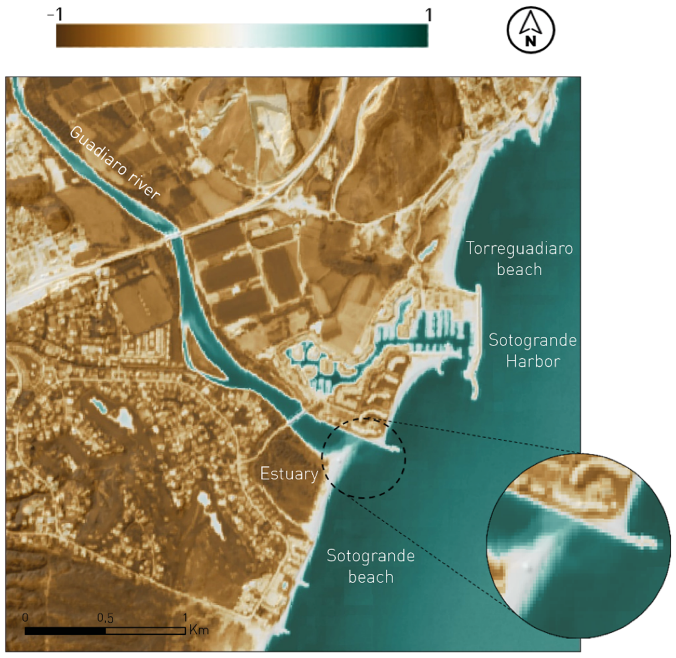
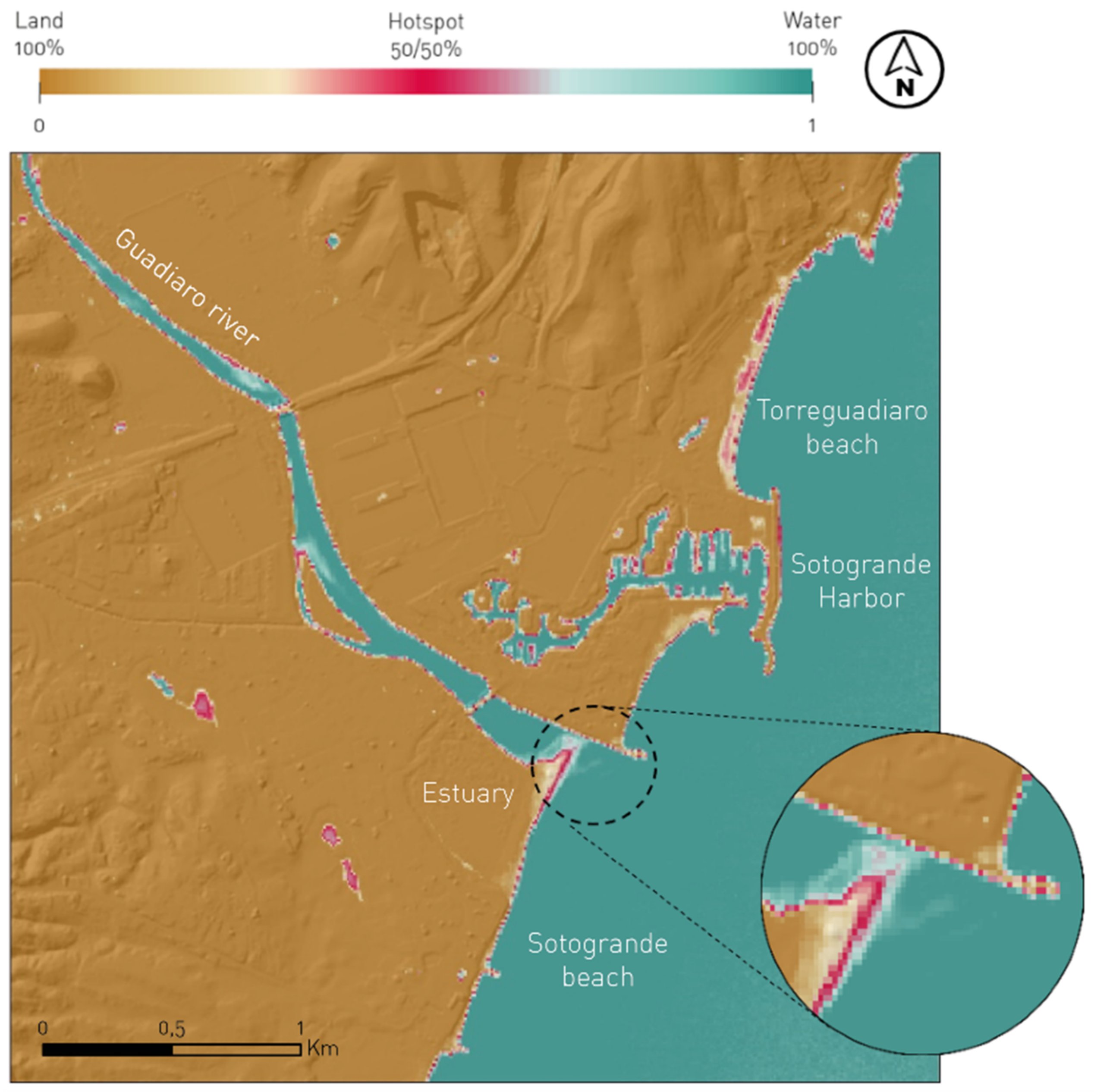
2.3.2. Sea–Land Mapping

Once the images were pre-processed and stored in the new Image Collection, in order to study the morpho-dynamical variability of the Guadiaro sand spit through sea–land mapping, the NDWI was applied (Figure 4). The NDWI was proposed by McFeeters [45], designed to maximize the reflectance of the water body in the green band ( ρ 3) (559 nm) and minimize the reflectance of the water body in the near infrared (NIR) band ( ρ 8) (864 nm) (1), with a range value from −1 and +1.
NDWI = ρ 3   ρ 8 ρ 3 +   ρ 8
Two main analyses were performed using NDWI in order to characterize the sand spit of the Guadiaro river and the adjacent beaches. Firstly, mean values were calculated obtaining climatologies for the whole period (2017–2020) and for each year in the whole AOI and, seasonality mean values for the sand spit zone to analyze seasonal trends (code available in GEE: https://code.earthengine.google.com/7b779ffe4fd2526bfd7397c1a9383206, accessed on 1 February 2021). The climatology concept refers to the average for all the raster, a geoprocessed S2 L2A image with applied NDWI index in our case, available from spring 2017 to autumn 2020. Secondly, in order to identify hotspot for accretion and erosion trends, Variation Rates (VR) between sea and land pixels were performed for the AOI (code available in GEE: https://code.earthengine.google.com/414fc98a57150171490c6f1fb909ca16, accessed on 1 February 2021). In this last case, NDWI threshold was used to discretize pixels into Boolean data (0: land; 1: ocean), for which thresholds between 0.05 to 0.15 were tested, revealing the 0.1 threshold value as an optimized coastline lineation for single images. However, when computing several images, 0.1 threshold included too much data noise in the ocean and river area, not properly distinguishing the coastline, and needing to use a threshold with value 0 for multi-image mining. Hence, it is important to highlight that, when working with a single image, threshold of 0.1 obtained the most accurate segmentation of land–water.
During value mining, a NDWI value for each case was added as a new parameter in the metadata Image Collection, with continuous values from −1 to 1 for climatologies (−1: permanent land; 1: permanent water) and between 0 and 1 for VR (0: permanent land; 1: permanent water). Finally, all the results were visualized in GEE and downloaded to Google Drive as a GeoTIFF image, ready for custom visualizations to be produced in ArcGIS Pro 2.5. The computational analysis was structured in three temporal scales for both Climatologies and VR: (1) total period (2017–2020); annual results for each year (2017, 2018, 2019, 2020); and analysis for each season, each year (from spring 2017 to autumn 2020).

3. Results

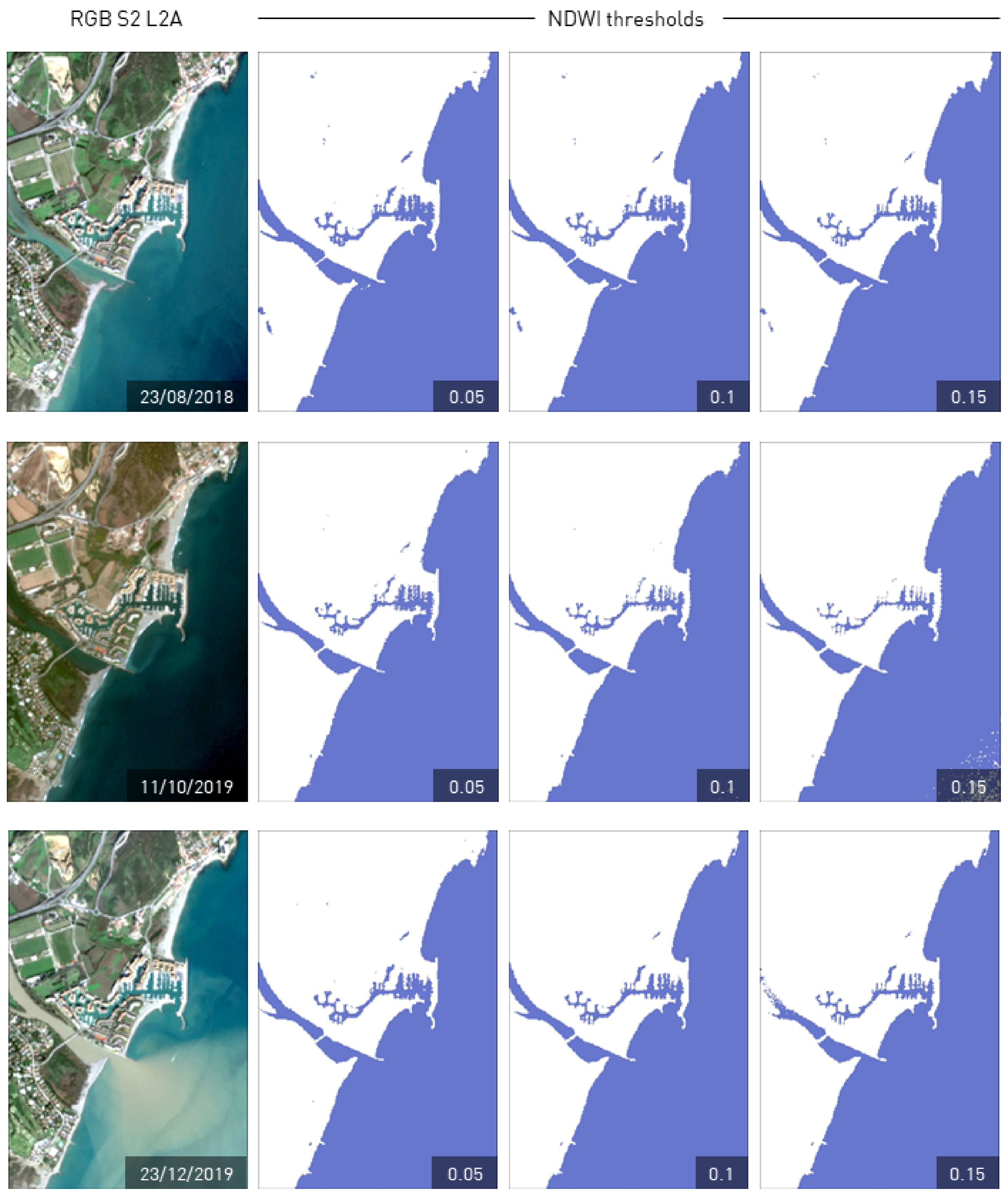
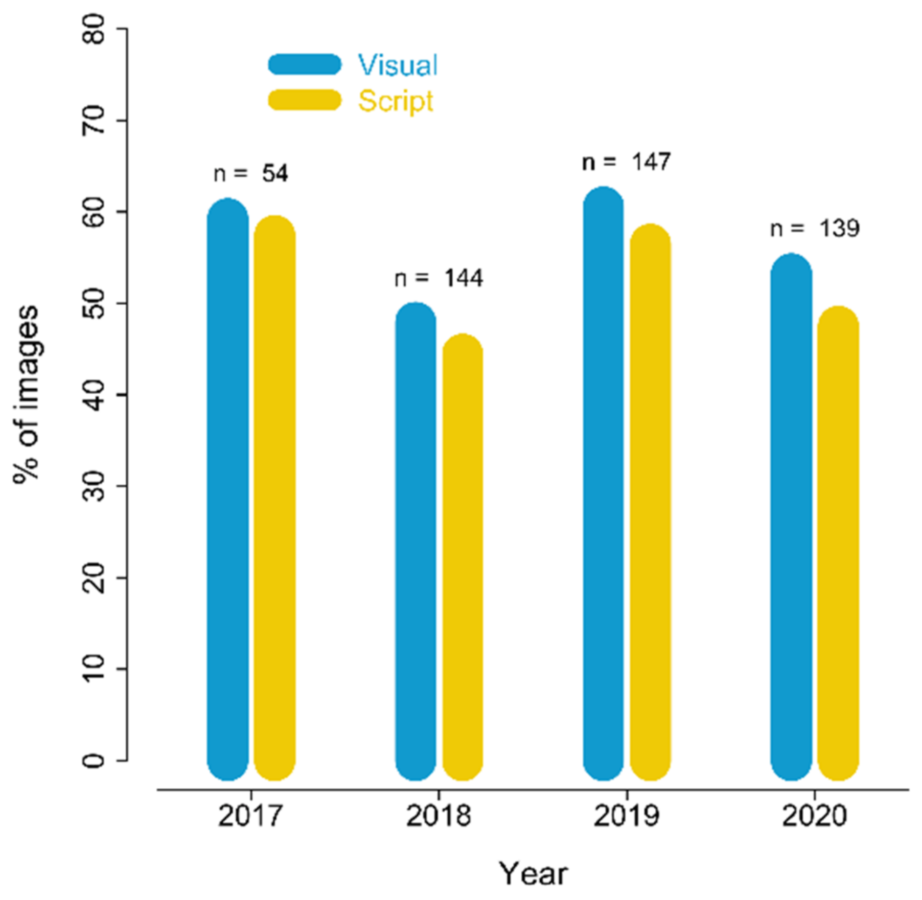
3.1. Cloud-Free Image Selection and Thresholding

The chart (Figure 5) shows image selection from both qualitative (EO Browser) and quantitative (GEE) methods, to validate GEE script accuracy, with a 15% maximum cloud probability applied. The percentage shows the number of images selected from the original GEE “COPERNICUS/S2_SR” dataset for each year, showing an optimal performance of the method. From a total of 484 images in the original dataset, 244 images (50.4%) were selected through the GEE algorithm and 264 images (54.5%) were selected using EO Browser, as a qualitative selection. All images selected with the GEE script were also selected visually, proving a 95% reliability and effectiveness with the GEE unsupervised image selection and, therefore, validating the methodology. This selection is accurate and consistent due to the fact that the cloud cover percentage is recalculated for all images in the AOI, not using the pre-calculated cloud cover percentage of the entire tile for filtering. For more detail, cloud cover validation percentages for each season can be seen in Table 1.
Concerning the evaluation of the NDWI threshold, three different values in critical cases were tested (0.05, 0.1 and 0.15) (Appendix A. Figure A1). The 0.1 value was used as an optimal NDWI, allowing us to detect the sand spit in the closed river mouth, just before closing, and the appearance of additional and smaller sand bars formed by local currents.

3.2. Climatology and Seasonality

The general climatology (2017–2020) in Figure 6 shows a mean sand spit position with a mostly closed river mouth, variating in its upper third and demonstrating its tendency to block water renewal in the estuary. Rigidity of both sides of the riverbed caused by urbanization blocked natural evolution, behaving more like a lagoon than an estuary. The NDWI index perfectly delimited the boundary between sand and water. River silting areas are observed along the riverbed extremely shallow depths during certain periods of the year, slowing water flow and increasing the accumulation of sedimentation in the river mouth.
Figure 7 shows annual climatologies, where high sand spit variability is clearly observed, proving how often the sand spit closes the river mouth during the year, especially for 2017, where the system is frequently working as a lagoon, a behavior that is repeated in 2020. Diversity of sand bar morphologies indicates no clear patterns. However, in both 2018 and 2019 an additional small sand bar was generated towards the ocean along the coast.
When evaluating seasonal climatologies (Figure 8), a variety of sand spit morphologies were observed. Similar to annual climatologies, seasonal means do not show patterns for opened or closed river mouth scenarios linked to any time particular of year. During 2017, the sand spit tended to be homogeneously closed. However, in 2018, a smaller secondary sand bar was generated because of the eddy effect, both bars merging in winter 2019. From spring 2019 until the end of the year the river mouth remained partially closed until it was completely closed by summer 2019, remaining closed for the following 6 months. Finally, after being opened by torrential rains, a new stable sand spit with U-shape morphology appeared in 2020 almost completely closing the river mouth. These rapidly changing dynamics reflect the complexity of the area and the importance of addressing estuarine problems from a holistic perspective, including natural processes and human activities from the river basin, the coastal zone and the ocean, as explained later in the Discussion Section 4.2.

3.3. Variation Rate

Once the spatio-temporal patterns were characterized, ranging from the riverbed to beaches and finally to the dynamic sand spit in the river mouth, in order to quantify this coastline variability, another study was carried out to evaluate its temporal and spatial variation. The VR identifies the most variable coastal areas in terms of land/water mapping pixels. This estimation has values from 0 (referred to pixels that are always land) to 1 (referred to pixels that are always water), the middle value (0.5) being areas of maximum variation. Light blue values show pixel covered by water for a longer time, while light brown values show the opposite trend. To evaluate the same temporal scales, this section follows the same structure as Section 3.2.
Variation Rate for the study period (2017–2020) (Figure 9) identifies two main hotspot areas of high variability. Firstly, the sand spit boundaries between land and water, with a water buffer in the upper third of its a pointed morphology; and secondly, Torreguadiaro beach, northwards of Sotogrande harbor. Torreguadiaro beach shows general instability due to the presence of small temporal lagoons created by maritime storms and waves, whose presence has been confirmed by RGB high-resolution images and in situ observations. Therefore, S2 images are detecting high soil moisture in the sandy areas and water accumulation in the rocky areas of Torreguadiaro beach. However, no significant variations are observed in Sotogrande beach and Guadiaro estuary between 2017 and 2020.
The correlation into temporal patterns can be very useful for coastal managers when designing adaptive policies against erosion and artificial river mouth openings. For this reason, as done in the climatology section, in order to understand whether areas of high variability followed any temporal pattern, annual and seasonal VR maps were generated between 2017 and 2020.
Generally, annual VR for the land–sea interface also shows short-term sediment stability for Sotogrande beach (Figure 10). Moreover, when looking at the adjacent beach south of Sotogrande harbor, 2017 was also the only year presenting high sediment variability, while Torreguadiaro beach showed a general instability trend for the 4 years of the study.
However, annual VR for Guadiaro coastal sand spit showed how a small secondary sand bars existing in 2018 and 2019 were unstable and of short duration. Moreover, no patterns of external or internal variability of the bar are observed, varying externally in 2019, internally in 2018 and 2020, and homogeneously in 2017.
Figure 11 shows how the sand spit varies between seasons. Summer showed a high variability between years, most likely due to artificial openings in times of increased touristic activity as an operational response to eutrophication episodes. Days with the sand spit closed, resulting in poor renewed water together with high temperatures, are associated with phytoplankton blooms, anoxia and high mortality of marine flora and fauna [59]. The days with the river mouth closed in a drought period, the typical rainfall hydrographic regime of the Mediterranean climate, the estuary works similar to a coastal lagoon [14].

4. Discussion and Conclusions

4.1. High Frequency Remote Sensing Data: S2, GEE and NDWI

Coastal environments are constantly changing and their continuous monitoring is key to proper evaluation and management. Estuaries and coastal lagoons are vulnerable environments affected by atrophic impacts and climate change; therefore, monitoring efforts are crucial for their conservation. By applying remote sensing techniques, consistent and robust methodologies for sea–land mapping and coastline detection were recently obtained on a global scale [22,25,29,48,60,61]. However, heterogeneity of sea–land mapping and coastline delineation methods and the difficult access to these tools by coastal managers usually restricts their use [24,35,36,40,62,63]. The potential of GEE has already been demonstrated in previous studies [37,38,60,64,65], and we used S2 images within GEE in order to ensure accuracy and robust performance, as well as a user-friendly and accessible tool for coastal managers.
Research studies of spatio-temporal variability of sand spit formations and evolution of nearby beaches are crucial for understanding the adaptation of estuarine systems under multiple anthropogenic pressures. In the Guadiaro estuary, eutrophication events have been connected to the lack of water renewal commonly promoted by sand spit closure since 1970s, where earlier studies employed low-frequency data sampling [9,10,11,12]. Thanks to the 10 m spatial resolution of S2, sea–land mapping has been successfully accomplished. Moreover, recent studies of S2 pixel accuracy have demonstrated upscaling improvements up to 2.5 m of spatial resolution [66], a substantial improvement paving the way for the use of S2 in the future of coastal monitoring. The methodology used in this study can be implemented for monitoring sand spit and beach variability for qualitative evaluation, with images available since 30 March 2017 (since 2015 with L1C). This is the first study in the Guadiaro estuary using S2-A/B imagery for coastal proposes as well as using the GEE platform for analytics. Previous studies used aerial imagery to inspect the Guadiaro river mouth modelling both northern and southern beaches [10,12,14], but not satellite imagery. Video-imaging techniques provide high-frequency data, albeit with a limited spatial coverage as fixed and site-specific ground-based technologies [67].
The method proposed in this study is completely automatic and cloud-based, avoiding the need to download each satellite image as well as intermediate steps during geoprocessing, in contrast to the CoastSat methodology [36]. Firstly, it has an automated workflow for selecting S2 L2A satellite imagery with low custom cloud cover with 95% reliability. This approach indicated consistency in performance for cloud-free image selection as a result of the recalculation of image cloud cover after cropping the AOI. Contrary to those commonly used in other studies [38], this approach does not take predefined cloud cover values from GEE for the entire tile. Furthermore, automatic sea–land mapping has many advantages over traditional methods. While manual shoreline delimitation is more accurate, it is labor-intensive and time-consuming [40], and, therefore, not the optimal option for high-frequency and long-term monitoring. However, as already demonstrated in previous studies, the use of indices for automatic sea–land mapping is biased towards false classification pixels due to clouds and breaking waves [41]. For this reason, optimization of image selection and cloud masking is key, and this study advances this field by achieved accurate results, offering a ready to use method for coastal monitoring that also generates useful information for the complete coastal management cycle on a global scale.
According to McAllister et al., the use of S2 for shoreline extraction through water and non-water pixels between 2006 and 2021 revealed a better performance of water indices and thresholding [68]. Among indices, NDWI and MNDWI are the most commonly used due to their optimized performance [43,44,49,51,69], having been subjected to different modifications [70], while thresholding is widely considered to be the simplest method of image segmentation [68]. We used the first NDWI defined by McFeeters [45], as MNDWI enhances the performance for coastal shadows (e.g., cliffs) and it can reveal more detail in open water [68,70], our study being focused on flat beaches and sand spit morphologies along the coast. Regarding NDWI threshold, this study revealed an optimized 0.1 value for single images, while the threshold value of 0 revealed less data noise for long temporal statistics. According to Xu [70], “threshold values for MNDWI to achieve best water extraction results are usually much less than those of NDWI, suggesting using zero as a default threshold value can produce better water extraction accuracy for the MNDWI than for the NDWI“. However, while we demonstrated 0.1 is suitable for single-image processing, the application of a 0 threshold in NDWI for computing statistics among several images revealed better water and non-water mapping; furthermore, other studies also refer to 0 threshold as the best performance for large spatial extents [71].

4.2. Contributions to Coastal Management

Regarding the Guadiaro river mouth, this study is essential for understanding external pressures and effects, as well as the natural dynamics of the sand spit, whose spatial distribution is highly conditioned by the river and ocean systems [11]. Applying S2 L2A satellite imagery we developed a monitoring tool that allows selection of the most optimal technique available to manage and prevent the closure of the river mouth in early stages, improving its temporal and economic efficiency, as well as to re-evaluate over time the suitability of the management measures applied. Additionally, the effectiveness of artificial openings in the short-term shown in Figure 3 could not be demonstrated, since images immediately before and after the three artificial openings corresponding to 2017 and 2018 were covered by clouds, and by 2019 and 2020 dredging was not necessary, as reported by the Spanish Government. However, further monitoring over time can reveal more insights. Only relatively short-term data are available for this study (2017–2020), hindering the overview of seasonal trends, with a large portion of estuaries depending mostly on upstream anthropogenic impacts [72]. While Landsat mission imagery offers historical data, its spatial resolution (30 m) is not suitable for small sand spits that require increased spatial detail, compared to the 10 m spatial resolution provided by the S2-A/B twin satellites. Moreover, the S2 5-day high-revisit frequency at the Equator (better at higher latitude) allows more accurate detection of changes in the sand spit in the immediate term after a rainfall event, compared with the 16-day revisit of Landsat-8. These characteristics position S2-A/B satellites in the present and future for coastal monitoring.
For the Guadiaro river mouth, the sand spit, and the surrounding beaches, we achieved the following results: (1) regarding the sand spit, especially in 2020 it remained closed throughout the summer season, most likely associated with the COVID-19 pandemic, during which many international tourists were not able to visit Sotogrande, reducing anthropogenic pressure, including urban waste; (2) through climatologies we evaluate how additional small sand bars could be caused by the northward longitudinal current blocked after the construction of Sotogrande harbor; (3) [55] replenishing of beaches can also be detected and monitored by means of S2 images, as demonstrated in the variability of the beach to the south of the Port of Sotogrande in 2017; and (4) the land–sea interface of sandy beaches is more easily identified in different studies throughout the globe compared to rocky beaches or coastal cliffs [36,61,73,74], mostly due to image spatial resolution [75]. However, while S2 undoubtedly enhanced its spatial resolution up to 10 m and, consequently, enhancing the rocky beach delineation, other effects, such as the presence of natural areas of water accumulation on the rocky beach, can lead to misinterpretation, as happened on the Torreguadiaro beach. In summary, the presented optimized monitoring tool can not only be used as an early-warning system for preventing closure episodes, but also for evaluating past measures and future management strategies.
Accordingly, integrated coastal management requires information throughout the entire management cycle [14,15,16,17]. Our monitoring tool can provide the necessary information for each management stage. At the beginning, information is required to make a diagnosis of the problems and impacts to be faced by the planning initiative. This will allow the formulation of suitable tools for coastal management. Information is also needed during the implementation of the management program, so adjustments can be made in order to improve its development. As an example, it is possible to assess if a coastal or watershed plan is given the desired results in the estuarine area in the short, medium or long term. Finally, it is extremely important to have information from the monitoring of the complete planning cycle during the evaluation phase. At this stage, the results are assessed and some questions must be answered: Have we achieved the objectives? Are we in the desired scenario? What are the main difficulties we have faced? What can be improved in the next planning cycle?
Among the advantages of the monitoring tool for coastal management, the followings can be highlighted: (a) A coastal management program is a result of a public policy. In this sense, and according to Olsen [76], it is important to have well defined and unambiguous goals, so progress towards to its achievement can be measured. The monitoring tool is able to provide long-term sustained information helping to assess, adapt, evaluate and improve such policy objectives; (b) an adaptive ecosystem-based management approach requires sustained monitoring [18,19,20]. The presented monitoring tool can provide a cost-effective early warning system each 5 days (without cloud coverage), facilitating adaptive management in the area. In this sense, it is possible to correlate the changes of state measured in the estuarine area with the responses given by the administration [21]; (c) the Guadiaro estuarine area shows the result of several sectoral policies: ports, watershed, mining, tourism, agriculture, among others. Although the closure of the river mouth is part of a natural process due to the effect of the maritime climate and the waves in the sand spit, uncoordinated sectoral planning frequently results in a cumulative effect of closures and severe eutrophication episodes. Information about sand spit trends can be related with the effects of different policy cycles. This knowledge can be used to support the development of a joint policy in the studied area.
In conclusion, the method proposed is simple and easily transferable to other environments on a global scale, with the scripts being open access, online, and ready to use. This tool provides continuous and long-term critical information and analysis through sea–land mapping assessing coastal zone response, approaching this technology as an accessible tool for coastal managers, and supporting daily operative and strategic management. This implementation ensures continuous and detailed monitoring in order to support an ecosystem-based approach for estuarine areas, and provides an added value that can encourage optimal decision making.

Author Contributions

Conceptualization, M.R., G.N., J.G.-S. and I.C.; methodology, software, validation and formal analysis, M.R.; writing—original draft preparation, M.R.; writing—review, editing and supervision, G.N., J.G.-S. and I.C.; project administration, G.N. and I.C.; funding acquisition, M.R., G.N. and I.C. All authors have read and agreed to the published version of the manuscript.

Funding

This research was funded by RTI2018-098784-J-I00 Sen2Coast project by the MCIN/AEI/10.13039/501100011033 and by “ERDF A way of making Europe”, by grant IJC2019-039382-I (Juan de la Cierva-Incorporación) by the Ministry of Science and Innovation of the Spanish Government, by grants FPU20/01294 and JAEINT_20_00462 (JAE INTRO 2020) by the Ministry of Universities of the Spanish Government and by PY20-00244 Sat4Algae project by the Andalusian Regional Government (Junta de Andalucía).

Institutional Review Board Statement

Not applicable.

Informed Consent Statement

Not applicable.

Data Availability Statement

Publicly available datasets were analyzed in this study, accessible through GEE [https://developers.google.com/earth-engine/datasets/catalog/COPERNICUS_S2_SR, accessed on 1 February 2021 and https://developers.google.com/earth-engine/datasets/catalog/COPERNICUS_S2_CLOUD_PROBABILITY, accessed on 1 February 2021]. The three GEE scripts can be found as follows: (1) for cloud-free image selection [https://code.earthengine.google.com/6363973f5918f3eacd09d890a52f5827, accessed on 1 February 2021]; (2) for climatology analysis [https://code.earthengine.google.com/7b779ffe4fd2526bfd7397c1a9383206, accessed on 1 February 2021]; and (3) for VR analysis [https://code.earthengine.google.com/414fc98a57150171490c6f1fb909ca16, accessed on 1 February 2021].

Acknowledgments

We would like to thank the European Space Agency, the European Commission and the Copernicus programme for distributing Sentinel-2 imagery; Google for developing the Google Earth Engine cloud computing platform, for its data accessibility and computational capacity freely available for researchers; Patricio Poullet Brea and Gregorio Gómez Pina, from the Coastal Office in the Atlantic Andalusia Ministry of Environment, for supporting this project as a pilot to monitor estuaries in Andalusia, as well as for the technical data provided; and Martha Bonnet Dunbar for the English language revision. This work represents a contribution to the CSIC Thematic Interdisciplinary Platform PTI TELEDETECT.

Conflicts of Interest

The authors declare no conflict of interest.

Appendix A

Figure A1. NDWI thresholding test showing 0.1 value as optimal. Image from 23 August 2018 shows the delineation of an additional sand bar; second image (11 October 2019) shows the detection of the sand spit closing the river mouth; and last image (23 December 2019) shows how scenarios with high turbidity do not interfere in water and non-water pixel classification.
Remotesensing 14 02345 g0a1

References

  1. Lotze, H.K.; Lenihan, H.S.; Bourque, B.J.; Bradbury, R.H.; Cooke, R.G.; Kay, M.C.; Kidwell, S.M.; Kirby, M.X.; Peterson, C.H.; Jackson, J.B. Depletion, degradation, and recovery potential of estuaries and coastal seas. Science 2006, 312, 1806–1809. [Google Scholar] [CrossRef]
  2. Meybeck, M. Carbon, nitrogen, and phosphorus transport by world rivers. Am. J. Sci. 1982, 282, 401–450. [Google Scholar] [CrossRef]
  3. Rao, N.S.; Ghermandi, A.; Portela, R.; Wang, X. Global values of coastal ecosystem services: A spatial economic analysis of shoreline protection values. Ecosyst. Serv. 2015, 11, 95–105. [Google Scholar] [CrossRef]
  4. Fragkias, M.; Seto, K.C. The rise and rise of urban expansion. Glob. Chang. 2012, 78, 16–19. [Google Scholar]
  5. Neumann, B.; Vafeidis, A.T.; Zimmermann, J.; Nicholls, R.J. Future coastal population growth and exposure to sea-level rise and coastal flooding-a global assessment. PLoS ONE 2015, 10, e0118571. [Google Scholar] [CrossRef] [Green Version]
  6. Erena, M.; Domínguez, J.A.; Aguado-Giménez, F.; Soria, J.; García-Galiano, S. Monitoring Coastal Lagoon Water Quality through Remote Sensing: The Mar Menor as a Case Study. Water 2019, 11, 1468. [Google Scholar] [CrossRef] [Green Version]
  7. Sòria-Perpinyà, X.; Miracle, M.R.; Soria, J.; Delegido, J.; Vicente, E. Remote sensing application for the study of rapid flushing to remediate eutrophication in shallow lagoons (Albufera of Valencia). Hydrobiologia 2019, 829, 125–132. [Google Scholar] [CrossRef]
  8. Mills, A.K.; Bolte, J.P.; Ruggiero, P.; Serafin, K.A.; Lipiec, E.; Corcoran, P.; Stevenson, J.; Zanocco, C.; Lach, D. Exploring the impacts of climate and policy changes on coastal community resilience: Simulating alternative future scenarios. Environ. Model. Softw. 2018, 109, 80–92. [Google Scholar] [CrossRef] [Green Version]
  9. Caballero, I.; Chapela-Bernatche, L.; Roque-Atienza, D.; Tejedor Álvarez, M.B.; Gomez-Pina, G.; Muñoz Pérez, J.J. Influencia del Oleaje en las Condiciones de Cierre de la Desembocadura del Río Guadiaro (Cádiz); IX Jornadas Españolas de Ingenieria de Costas y Puertos: Cadiz, Spain, 2008; pp. 32–39. [Google Scholar]
  10. Muñoz Pérez, J.J.; de la Casa, Á.; Gomez-Pina, G.; Acha Martin, A. Environmental Restoration of the Guadiaro River Estuary, Cadiz, Spain. Period. Biol. 2000, 102, 333–338. [Google Scholar]
  11. Román-Sierra, J.; Navarro-Pons, M.; Muñoz Pérez, J.J.; Tejedor Álvarez, M.B.; Física, A. Variabilidad espacio-temporal de la flecha del río Guadiaro. In Spatial and Temporal Variability in the Spif of Guadiaro River; Ingenieriía Civil: Madrid, Spain, 2008; Volume 149, pp. 111–122. ISSN 0213-8468. [Google Scholar]
  12. Diez, J.J.; Fernando, R.; Veiga, E.M. (Eds.) Coastal Impacts Around Guadiaro River Mouth (Spain). In Engineering Geology for Society and Territory; Springer International Publishing: Cham, Switzerland, 2014; Volume 4. [Google Scholar]
  13. Aleksandrov, S.V. Biological production and eutrophication of Baltic Sea estuarine ecosystems: The Curonian and Vistula Lagoons. Mar. Pollut. Bull. 2010, 61, 205–210. [Google Scholar] [CrossRef]
  14. Chica Ruiz, J.A.; Barragán Muñoz, J.M. Estado y Tendencia de los Servicios de los Ecosistemas Litorales de Andalucía; Universidad de Cádiz Rectorado: Cádiz, Spain, 2014. [Google Scholar]
  15. GESAMP. The Contributions of Science to Integrated Coastal Management; FAO: Rome, Italy, 1996. [Google Scholar]
  16. Barragán Muñoz, J.M. Coastal management and public policy in Spain. Ocean. Coast. Manag. 2010, 53, 209–217. [Google Scholar] [CrossRef]
  17. Barragán, J.M. Política, Gestión y Litoral: Una Nueva Visión de la Gestión Integrada de Áreas Litorales; Flores: Cadiz, Spain, 2014; 685p. [Google Scholar]
  18. Barragán, J.M.; Lazo, Ó. Policy progress on ICZM in Peru. Ocean Coast. Manag. 2018, 157, 203–216. [Google Scholar] [CrossRef]
  19. Barragán Muñoz, J.M. Progress of coastal management in Latin America and the Caribbean. Ocean Coast. Manag. 2020, 184, 105009. [Google Scholar] [CrossRef]
  20. Nava Fuentes, J.C.; Arenas Granados, P.; Martins, F.C. Coastal management in Mexico: Improvements after the marine and coastal policy publication. Ocean Coast. Manag. 2017, 137, 131–143. [Google Scholar] [CrossRef]
  21. Elliott, M. The role of the DPSIR approach and conceptual models in marine environmental management: An example for offshore wind power. Mar. Pollut. Bull. 2002, 6, 3–7. [Google Scholar] [CrossRef]
  22. Pardo-Pascual, J.E.; Sánchez-García, E.; Almonacid-Caballer, J.; Palomar-Vázquez, J.M.; Priego de los Santos, E.; Fernández-Sarría, A.; Balaguer-Beser, Á. Assessing the Accuracy of Automatically Extracted Shorelines on Microtidal Beaches from Landsat 7, Landsat 8 and Sentinel-2 Imagery. Remote Sens. 2018, 10, 326. [Google Scholar] [CrossRef] [Green Version]
  23. Taveneau, A.; Almar, R.; Bergsma, E.W.J.; Sy, B.A.; Ndour, A.; Sadio, M.; Garlan, T. Observing and Predicting Coastal Erosion at the Langue de Barbarie Sand Spit around Saint Louis (Senegal, West Africa) through Satellite-Derived Digital Elevation Model and Shoreline. Remote Sens. 2021, 13, 2454. [Google Scholar] [CrossRef]
  24. Quang Tuan, N.; Cong Tin, H.; Quang Doc, L.; Anh Tuan, T. Historical Monitoring of Shoreline Changes in the Cua Dai Estuary, Central Vietnam Using Multi-Temporal Remote Sensing Data. Geosciences 2017, 7, 72. [Google Scholar] [CrossRef] [Green Version]
  25. Splinter, K.D.; Harley, M.D.; Turner, I.L. Remote Sensing is Changing Our View of the Coast: Insights from 40 Years of Monitoring at Narrabeen-Collaroy, Australia. Remote Sens. 2018, 10, 1744. [Google Scholar] [CrossRef] [Green Version]
  26. Caballero, I.; Fernández, R.; Escalante, O.M.; Mamán, L.; Navarro, G. New capabilities of Sentinel-2A/B satellites combined with in situ data for monitoring small harmful algal blooms in complex coastal waters. Sci. Rep. 2020, 10, 8743. [Google Scholar] [CrossRef]
  27. Caballero, I.; Stumpf, R.P. On the use of Sentinel-2 satellites and lidar surveys for the change detection of shallow bathymetry: The case study of North Carolina inlets. Coast. Eng. 2021, 169, 103936. [Google Scholar] [CrossRef]
  28. Traganos, D.; Reinartz, P. Mapping Mediterranean seagrasses with Sentinel-2 imagery. Mar. Pollut. Bull. 2018, 134, 197–209. [Google Scholar] [CrossRef] [Green Version]
  29. Cabezas-Rabadán, C.; Pardo-Pascual, J.E.; Palomar-Vázquez, J.; Fernández-Sarría, A. Characterizing beach changes using high-frequency Sentinel-2 derived shorelines on the Valencian coast (Spanish Mediterranean). Sci. Total Environ. 2019, 691, 216–231. [Google Scholar] [CrossRef]
  30. Whitehead, B.; Andrews, D.; Shah, A.; Maidment, G. Assessing the environmental impact of data centres part 1: Background, energy use and metrics. Build. Environ. 2014, 82, 151–159. [Google Scholar] [CrossRef]
  31. Gorelick, N.; Hancher, M.; Dixon, M.; Ilyushchenko, S.; Thau, D.; Moore, R. Google Earth Engine: Planetary-scale geospatial analysis for everyone. Remote Sens. Environ. 2017, 202, 18–27. [Google Scholar] [CrossRef]
  32. Amani, M.; Ghorbanian, A.; Ahmadi, S.A.; Kakooei, M.; Moghimi, A.; Mirmazloumi, S.M.; Moghaddam, S.H.A.; Mahdavi, S.; Ghahremanloo, M.; Parsian, S.; et al. Google Earth Engine Cloud Computing Platform for Remote Sensing Big Data Applications: A Comprehensive Review. IEEE J. Sel. Top. Appl. Earth Obs. Remote Sens. 2020, 13, 5326–5350. [Google Scholar] [CrossRef]
  33. Caballero, I.; Navarro, G. Monitoring cyanoHABs and water quality in Laguna Lake (Philippines) with Sentinel-2 satellites during the 2020 Pacific typhoon season. Sci. Total Environ. 2021, 788, 147700. [Google Scholar] [CrossRef]
  34. Bioresita, F.; Ummah, M.H.; Wulansari, M.; Putri, N.A. (Eds.) Monitoring Seawater Quality in the Kali Porong Estuary as an Area for Lapindo Mud Disposal leveraging Google Earth Engine. In IOP Conference Series: Earth and Environmental Science; IOP Publishing: Bristol, UK, 2021. [Google Scholar]
  35. Vos, K.; Harley, M.D.; Splinter, K.D.; Simmons, J.A.; Turner, I.L. Sub-annual to multi-decadal shoreline variability from publicly available satellite imagery. Coast. Eng. 2019, 150, 160–174. [Google Scholar] [CrossRef]
  36. Vos, K.; Splinter, K.D.; Harley, M.D.; Simmons, J.A.; Turner, I.L. CoastSat: A Google Earth Engine-enabled Python toolkit to extract shorelines from publicly available satellite imagery. Environ. Model. Softw. 2019, 122, 104528. [Google Scholar] [CrossRef]
  37. Terres de Lima, L.; Fernández-Fernández, S.; Gonçalves, J.F.; Magalhães Filho, L.; Bernardes, C. Development of Tools for Coastal Management in Google Earth Engine: Uncertainty Bathtub Model and Bruun Rule. Remote Sens. 2021, 13, 1424. [Google Scholar] [CrossRef]
  38. Hird, J.N.; DeLancey, E.R.; McDermid, G.J.; Kariyeva, J. Google Earth Engine, Open-Access Satellite Data, and Machine Learning in Support of Large-Area Probabilistic Wetland Mapping. Remote Sens. 2017, 9, 1315. [Google Scholar] [CrossRef] [Green Version]
  39. De Muro, S.; Ibba, A.; Simeone, S.; Buosi, C.; Brambilla, W. An integrated sea-land approach for mapping geomorphological and sedimentological features in an urban microtidal wave-dominated beach: A case study from S Sardinia, western Mediterranean. J. Maps 2017, 13, 822–835. [Google Scholar] [CrossRef] [Green Version]
  40. Rodríguez-Santalla, I.; Roca, M.; Martínez-Clavel, B.; Pablo, M.; Moreno-Blasco, L.; Blázquez, A.M. Coastal changes between the harbours of Castellón and Sagunto (Spain) from the mid-twentieth century to present. Reg. Stud. Mar. Sci. 2021, 46, 101905. [Google Scholar] [CrossRef]
  41. Adebisi, N.; Balogun, A.-L.; Mahdianpari, M.; Min, T.H. Assessing the Impacts of Rising Sea Level on Coastal Morpho-Dynamics with Automated High-Frequency Shoreline Mapping Using Multi-Sensor Optical Satellites. Remote Sens. 2021, 13, 3587. [Google Scholar] [CrossRef]
  42. Nazeer, M.; Waqas, M.; Shahzad, M.I.; Zia, I.; Wu, W. Coastline Vulnerability Assessment through Landsat and Cubesats in a Coastal Mega City. Remote Sens. 2020, 12, 749. [Google Scholar] [CrossRef] [Green Version]
  43. Fisher, A.; Flood, N.; Danaher, T. Comparing Landsat water index methods for automated water classification in eastern Australia. Remote Sens. Environ. 2016, 175, 167–182. [Google Scholar] [CrossRef]
  44. Latella, M.; Luijendijk, A.; Moreno-Rodenas, A.M.; Camporeale, C. Satellite Image Processing for the Coarse-Scale Investigation of Sandy Coastal Areas. Remote Sens. 2021, 13, 4613. [Google Scholar] [CrossRef]
  45. McFeeters, S.K. The use of the Normalized Difference Water Index (NDWI) in the delineation of open water features. Int. J. Remote Sens. 1996, 17, 1425–1432. [Google Scholar] [CrossRef]
  46. Kaplan, G.; Avdan, U. Object-based water body extraction model using Sentinel-2 satellite imagery. Eur. J. Remote Sens. 2017, 50, 137–143. [Google Scholar] [CrossRef] [Green Version]
  47. Murray, N.J.; Phinn, S.R.; Clemens, R.S.; Roelfsema, C.M.; Fuller, R.A. Continental scale mapping of tidal flats across East Asia using the Landsat archive. Remote Sens. 2012, 4, 3417–3426. [Google Scholar] [CrossRef] [Green Version]
  48. Wu, Q.; Miao, S.; Huang, H.; Guo, M.; Zhang, L.; Yang, L.; Zhou, C. Quantitative Analysis on Coastline Changes of Yangtze River Delta Based on High Spatial Resolution Remote Sensing Images. Remote Sens. 2022, 14, 310. [Google Scholar] [CrossRef]
  49. Feyisa, G.L.; Meilby, H.; Fensholt, R.; Proud, S.R. Automated Water Extraction Index: A new technique for surface water mapping using Landsat imagery. Remote Sens. Environ. 2014, 140, 23–35. [Google Scholar] [CrossRef]
  50. Wang, Z.; Liu, J.; Li, J.; Zhang, D.D. Multi-spectral water index (MuWI): A native 10-m multi-spectral water index for accurate water mapping on Sentinel-2. Remote Sens. 2018, 10, 1643. [Google Scholar] [CrossRef] [Green Version]
  51. Rokni, K.; Ahmad, A.; Selamat, A.; Hazini, S. Water Feature Extraction and Change Detection Using Multitemporal Landsat Imagery. Remote Sens. 2014, 6, 4173–4189. [Google Scholar] [CrossRef] [Green Version]
  52. Hayes, M.O. Barrier island morphology as a function of tidal and wave regime. In Barrier Islands; Leatherman, S.P., Ed.; Academic Press: New York, NY, USA, 1979. [Google Scholar]
  53. Muñoz-Pérez, J.J.; Caballero, I.; Tejedor, B.; Gomez-Pina, G. Reversal in longshore sediment transport without variations in wave power direction. J. Coast. Res. 2010, 26, 780–786. [Google Scholar] [CrossRef]
  54. Martín-Rodríguez, J.F.; Mudarra, M.; Andreo, B.; de la Torre, B.; Gil-Márquez, J.M.; Martín-Arias, J.; Nieto-López, J.M.; Prieto-Mera, J.; Rodríguez-Ruize, M.D. (Eds.) Monitoring and Preliminary Analysis of the Natural Responses Recorded in a Poorly Accessible Streambed Spring Located at a Fluviokarstic Gorge in Southern Spain; Springer International Publishing: Cham, Switzerland, 2020. [Google Scholar]
  55. Del Río, L.; Benavente, J.; Gracia, F.J.; Anfuso, G.; Aranda, M.; Montes, J.B.; Puig, M.; Talavera, L.; Plomaritis, T.A. Beaches of Cadiz. In The Spanish Coastal Systems: Dynamic Processes, Sediments and Management; Morales, J.A., Ed.; Springer International Publishing: Cham, Switzerland, 2019; pp. 311–334. [Google Scholar]
  56. Reguero, B.G.; Losada, I.J.; Méndez, F.J. A recent increase in global wave power as a consequence of oceanic warming. Nat. Commun. 2019, 10, 205. [Google Scholar] [CrossRef] [Green Version]
  57. Universidad de Cádiz (UCA). Gestión Integrada de Zonas Costeras y Cuencas Hidrográficas: Introducción a un Caso de Estudio. El Río Guadiaro. Grupo de Investigación en Gestión Integrada de Áreas Litorales. Convenio UCA-DGCOSTAS; Universidad de Cádiz (UCA): Cádiz, Spain, 2009. [Google Scholar]
  58. Rodríguez-Alarcón, R.; Lozano, S. A complex network analysis of Spanish river basins. J. Hydrol. 2019, 578, 124065. [Google Scholar] [CrossRef]
  59. Glibert, P.M.; Burkholder, J.M. The Complex Relationships Between Increases in Fertilization of the Earth, Coastal Eutrophication and Proliferation of Harmful Algal Blooms. In Ecology of Harmful Algae; Granéli, E., Turner, J.T., Eds.; Springer: Berlin/Heidelberg, Germany, 2006; pp. 341–354. [Google Scholar]
  60. Ding, Y.; Yang, X.; Jin, H.; Wang, Z.; Liu, Y.; Liu, B.; Zhang, J.; Liu, X.; Gao, K.; Meng, D. Monitoring Coastline Changes of the Malay Islands Based on Google Earth Engine and Dense Time-Series Remote Sensing Images. Remote Sens. 2021, 13, 3842. [Google Scholar] [CrossRef]
  61. Hagenaars, G.; de Vries, S.; Luijendijk, A.P.; de Boer, W.P.; Reniers, A.J.H.M. On the accuracy of automated shoreline detection derived from satellite imagery: A case study of the sand motor mega-scale nourishment. Coast. Eng. 2018, 133, 113–125. [Google Scholar] [CrossRef]
  62. Hu, X.; Wang, Y. Coastline Fractal Dimension of Mainland, Island, and Estuaries Using Multi-temporal Landsat Remote Sensing Data from 1978 to 2018: A Case Study of the Pearl River Estuary Area. Remote Sens. 2020, 12, 2482. [Google Scholar] [CrossRef]
  63. Smith, K.E.L.; Terrano, J.F.; Pitchford, J.L.; Archer, M.J. Coastal Wetland Shoreline Change Monitoring: A Comparison of Shorelines from High-Resolution WorldView Satellite Imagery, Aerial Imagery, and Field Surveys. Remote Sens. 2021, 13, 3030. [Google Scholar] [CrossRef]
  64. Dong, D.; Wang, C.; Yan, J.; He, Q.; Zeng, J.; Wei, Z. Combing Sentinel-1 and Sentinel-2 image time series for invasive Spartina alterniflora mapping on Google Earth Engine: A case study in Zhangjiang Estuary. J. Appl. Remote Sens. 2020, 14, 044504. [Google Scholar]
  65. Zhang, K.; Dong, X.; Liu, Z.; Gao, W.; Hu, Z.; Wu, G. Mapping Tidal Flats with Landsat 8 Images and Google Earth Engine: A Case Study of the China’s Eastern Coastal Zone circa 2015. Remote Sens. 2019, 11, 324. [Google Scholar] [CrossRef] [Green Version]
  66. Galar, M.; Sesma, R.; Ayala, C.; Albizua, L.; Aranda, C. Super-Resolution of Sentinel-2 Images Using Convolutional Neural Networks and Real Ground Truth Data. Remote Sens. 2020, 12, 2941. [Google Scholar] [CrossRef]
  67. Ribas, F.; Simarro, G.; Arriaga, J.; Luque, P. Automatic Shoreline Detection from Video Images by Combining Information from Different Methods. Remote Sens. 2020, 12, 3717. [Google Scholar] [CrossRef]
  68. McAllister, E.; Payo, A.; Novellino, A.; Dolphin, T.; Medina-Lopez, E. Multispectral satellite imagery and machine learning for the extraction of shoreline indicators. Coast. Eng. 2022, 174, 104102. [Google Scholar] [CrossRef]
  69. Du, Y.; Zhang, Y.; Ling, F.; Wang, Q.; Li, W.; Li, X. Water Bodies’ Mapping from Sentinel-2 Imagery with Modified Normalized Difference Water Index at 10-m Spatial Resolution Produced by Sharpening the SWIR Band. Remote Sens. 2016, 8, 354. [Google Scholar] [CrossRef] [Green Version]
  70. Xu, H. Modification of normalised difference water index (NDWI) to enhance open water features in remotely sensed imagery. Int. J. Remote Sens. 2006, 27, 3025–3033. [Google Scholar] [CrossRef]
  71. Bishop-Taylor, R.; Sagar, S.; Lymburner, L.; Alam, I.; Sixsmith, J. Sub-Pixel Waterline Extraction: Characterising Accuracy and Sensitivity to Indices and Spectra. Remote Sens. 2019, 11, 2984. [Google Scholar] [CrossRef] [Green Version]
  72. Sharp, J.H.; Yoshiyama, K.; Parker, A.E.; Schwartz, M.C.; Curless, S.E.; Beauregard, A.Y.; Ossolinski, J.E.; Davis, A.R. A Biogeochemical View of Estuarine Eutrophication: Seasonal and Spatial Trends and Correlations in the Delaware Estuary. Estuaries Coasts 2009, 32, 1023–1043. [Google Scholar] [CrossRef]
  73. Hagenaars, G.; Luijendijk, A.; de Vries, S.; de Boer, W. Long term coastline monitoring derived from satellite imagery. Proc. Coast. Dyn. 2017, 12–16, 1551–1562. [Google Scholar]
  74. Sekovski, I.; Stecchi, F.; Mancini, F.; Del Rio, L. Image classification methods applied to shoreline extraction on very high-resolution multispectral imagery. Int. J. Remote Sens. 2014, 35, 3556–3578. [Google Scholar] [CrossRef]
  75. Chen, D.; Stow, D.A.; Gong, P. Examining the effect of spatial resolution and texture window size on classification accuracy: An urban environment case. Int. J. Remote Sens. 2004, 25, 2177–2192. [Google Scholar] [CrossRef]
  76. Olsen, S.B. A Practitioner’s perspective on coastal ecosystem governance. In Integrated Coastal Zone Management; Wiley-Blackwell: Oxford, UK, 2009. [Google Scholar]
Figure 1. Satellite and aerial images from 1946 to 2019 showing the evolution of the Guadiaro estuary (source: PNOA).
Remotesensing 14 02345 g001
Figure 2. Study area: Guadiaro river mouth (San Roque, Cadiz), Spain.
Remotesensing 14 02345 g002
Figure 3. Guadiaro river mouth artificial openings from 2016 to 2018. Sand extraction volume (m3) and budget involved from the Spanish Government. There was no intervention during 2019 and 2020.
Remotesensing 14 02345 g003
Figure 4. Geoprocessing workflow in GEE with S2 L2A images. (a) low cloud cover probability image selection workflow; (b) NDWI index application and statistical geoprocessing workflow (climatology and VR).
Remotesensing 14 02345 g004
Figure 5. Workflow validation for cloud cover images. Percentage (%) of images selected in both methodologies to validate GEE script (n: number of images available in the image collection for each year. A total of 484 images were available before cloud-cover image filtering).
Remotesensing 14 02345 g005
Figure 6. Total climatology (2017–2020) using Sentinel-2 L2A images and NDWI index for the Gua-diaro river mouth. Scale 1:15,000.
Remotesensing 14 02345 g006
Figure 7. Annual climatologies using Sentinel-2 L2A images and NDWI index for the Guadiaro river mouth (single year means from 2017 to 2020). Scale 1:15,000.
Remotesensing 14 02345 g007
Figure 8. Seasonal climatologies using Sentinel-2 L2A images and NDWI index for the Guadiaro river mouth and its dynamic sand bar between spring 2017 and autumn 2020. Scale 1:3500.
Remotesensing 14 02345 g008
Figure 9. Variation rate of land/sea interface in the Guadiaro river mouth using Sentinel-2 L2A images and NDWI index between 2017 and 2020. Scale 1:15,000.
Remotesensing 14 02345 g009
Figure 10. Annual variation rate of land/sea interface in the Guadiaro river mouth using Sentinel-2 L2A images and NDWI index (single year VR from 2017 to 2020). Scale 1:15,000.
Remotesensing 14 02345 g010
Figure 11. Seasonal variation rate of land/sea interface in the Guadiaro river mouth using Sentinel-2 L2A images and NDWI index from 2017 to 2020. Sand spit variability. Scale 1:3500.
Remotesensing 14 02345 g011
Table 1. Seasonal number of images used for cloud-free image filtering validation. All images available, visual selection, automatic selection in GEE and percentages.
SeasonImages AvailableVisual SelectionAutomatic Filtering% Images Selected Visually *% Images Selected in GEE *
Spring 2017158753.346.7
Summer 201715101066.766.7
Autumn 201719131368.468.4
Winter 201834131338.238.2
Spring 201837141137.829.7
Summer 201835252171.460.0
Autumn 201836171747.247.2
Winter 201936171647.244.4
Spring 201936251969.452.8
Summer 201936272775.075.0
Autumn 201936201955.652.8
Winter 20203714937.824.3
Spring 202037171245.932.4
Summer 202037292878.475.7
Autumn 202032151546.946.9
* Percentage of selected images from available images in dataset (“COPERNICUS/S2_SR”). Image selection (visual or automated)/available images for corresponding season.
Publisher’s Note: MDPI stays neutral with regard to jurisdictional claims in published maps and institutional affiliations.

