Numerical Weather Predictions and Re-Analysis as Input for Lidar Inversions: Assessment of the Impact on Optical Products

Abstract

The atmospheric molecular number density can be obtained from atmospheric temperature and pressure profiles and is a significant input parameter for the inversion of lidar measurements. When measurements of vertical profiles of temperature and pressure are not available, atmospheric models are typically considered a valid alternative option. This paper investigates the influence of different atmospheric models (forecast and reanalysis) on the retrieval of aerosol optical properties (extinction and backscatter coefficients) by applying Raman and elastic-only methods to lidar measurements, to assess their use in lidar data processing. In general, reanalyzes are more accurate than forecasts, but, typically, they are not delivered in time for allowing near-real-time lidar data analysis. However, near-real-time observation is crucial for real-time monitoring of the environment and meteorological studies. The forecast models used in the paper are provided by the Integrated Forecasting System operated by the European Centre for Medium-Range Weather Forecasts (IFS_ECMWF) and the Global Data Assimilation System (GDAS), whereas the reanalysis model is obtained from the fifth-generation European Centre for Medium-Range Weather Forecasts ReAnalysis v5 (ERA5). The lidar dataset consists of measurements collected from four European Aerosol Research Lidar Network (EARLINET) stations during two intensive measurement campaigns and includes more than 200 cases at wavelengths of 355 nm, 532 nm, and 1064 nm. We present and discuss the results and influence of the forecast and reanalysis models in terms of deviations of the derived aerosol optical properties. The results show that the mean relative deviation in molecular number density is always below ±3%, while larger deviations are shown in the derived aerosol optical properties, and the size of the deviation depends on the retrieval method together with the different wavelengths. In general, the aerosol extinction coefficient retrieval is more dependent on the model used than the aerosol backscatter retrievals are. The larger influence on the extinction retrieval is mainly related to the deviation in the gradient of the temperature profile provided by forecast and reanalysis models rather than the absolute deviation of the molecular number density. We found that deviations in extinction were within ±5%, with a probability of 83% at 355 nm and 60% at 532 nm. Moreover, for aerosol backscatter coefficient retrievals, different models can have a larger impact when the backscatter coefficient is retrieved with the elastic method than when the backscatter coefficient is calculated using the Raman method at both 355 nm and 532 nm. In addition, the atmospheric aerosol load can also influence the deviations in the aerosol extinction and backscatter coefficients, showing a larger impact under low aerosol loading scenarios.

1. Introduction

At present, atmospheric aerosols are considered as one of the major sources of uncertainties in climate forcing [1]. There are many kinds of aerosols, each of which is characterized by specific optical properties. Most aerosols are generated by natural sources and human activities and greatly influence the Earth’s radiation balance [2]. For this reason, having a good knowledge of their global distribution, their vertical and horizontal extent, and their time of residence in the atmosphere is necessary for understanding their role in atmospheric processes [3,4] as well as human health [5,6] and the environment [7,8].

Lidar techniques have proven to be one of the most useful ways of obtaining atmospheric aerosol vertical profiles with high temporal and spatial resolution [9] and to identify multiple aerosol layers as well as their typology in the atmosphere [10,11]. In addition, with the developments in recent years in laser technology, measurement techniques, and data acquisition systems, lidar technology performance has greatly improved [12]. Several lidar techniques are suitable for atmospheric aerosol monitoring and study, such as elastic backscatter lidar and multi-wavelength Raman lidar. Elastic backscatter lidars detect only the elastic backscatter signals at the transmitted wavelength [13,14]. Two types of algorithms are typically used to retrieve profiles of the aerosol backscatter coefficient from the elastic backscattered signals: Klett–Fernald [15,16,17] and iterative [18,19]. Both algorithms require the assumption of the aerosol lidar ratio, i.e., the aerosol extinction-to-backscatter ratio, which is an important intensive parameter characterizing the aerosol type. An inappropriate aerosol lidar ratio value will introduce significant uncertainty in the retrieved results [20]. This limitation is overcome when multi-wavelength Raman lidar is used as these advanced systems detect not only elastic backscattered radiation but also radiation backscattered inelastically (Raman effect) by atmospheric Nitrogen molecules [21,22,23,24]. Multi-wavelength Raman lidar provides an independent measurement of the profiles of aerosol extinction and backscatter coefficients and, consequently, no assumption about the lidar ratio is required.

A single multi-wavelength Raman lidar system can be used to characterize the atmospheric aerosol content corresponding to a single observation point. Characterization on a larger horizontal scale can be achieved with coordinated lidar networks. The European Aerosol Research Lidar Network (EARLINET) was the first network to be established in 2000 with the main goal of providing the aerosol climatology over Europe [12,25,26]. Currently, EARLINET comprises 31 active lidar stations distributed over Europe, most of which operate multi-wavelength Raman lidars. A rigorous quality assurance program has been adopted to ensure a high level of quality and standardization of all EARLINET products [27,28,29,30]. Moreover, the EARLINET Single Calculus Chain (SCC) has been developed to provide all EARLINET stations with a tool for unsupervised, standardized, and quality assured data processing [31,32].

It should be noted that the molecular number density profile is also an important input parameter for the determination of the aerosol extinction and backscatter coefficient, both in Raman lidar systems and elastic backscatter lidar systems. Molecular number density profiles can be derived from vertical profiles of atmospheric temperature and pressure. Suitable vertical profiles can be measured by radiosonde when there is a radiosounding station close to the lidar station. The co-location in time and distance between lidar and sounding stations is an important aspect to consider. Although atmospheric pressure can be quite stable over time and horizontal location, the atmospheric temperature can differ considerably. Consequently, using radiosonde data measured several hours after/before the observations or kilometers apart from the lidar station can introduce non- negligible uncertainties in the lidar inversions. In addition, radiosoundings are usually quite expensive and typically they are launched two times per day, whereas, because lidar systems can operate 24/7, a more frequent sounding schedule would be preferable (e.g., hourly). Moreover, radiosoundings do not provide an exact vertical temperature and pressure profile above a station as they drift horizontally while ascending. For these reasons, the number density profiles to be used for input in lidar retrievals can also be obtained from temperature and pressure profiles provided by global atmospheric models (forecasts or reanalysis). The advantages with respect to radiosoundings are the increase in the temporal and spatial coverage, together with the verticality of the profiles provided. Furthermore, as forecasts or reanalysis models ingest all available radiosouding data, the accuracy of the provided temperature and pressure profiles is expected to be good enough to not impact too much on aerosol retrievals. However, different models are characterized by different accuracies, and the temporal resolution and spatial grid can be quite different. Reanalysis data are considered to be more accurate because they can ingest more observational data; however, reanalysis is usually made available after 1–2 months and, consequently, they cannot be used for the inversion of lidar observations in near-real-time. This limitation can be overcome by using model forecast data, which are made available in advance at the price of a lower accuracy.

To have a deeper understanding of the impact of using different forecast and reanalysis models on the EARLINET optical products, and to assess the corresponding uncertainties, the lidar data measured during the ACTRIS COVID-19 measurement campaign [33], and the EARLINET 72-h continuous observation campaign [26,34] were chosen. The results retrieved from two different atmospheric forecast models were analyzed: the Integrated Forecasting System operated by the European Centre for Medium-Range Weather Forecasts (IFS_ECMWF) and the Global Data Assimilation System (GDAS) produced by the US National Center for Environmental Prediction (NCEP), and these were compared with the results retrieved from the Atmospheric data from the fifth generation European Centre for Medium-Range Weather Forecasts ReAnalysis v5 (ERA5) model. Moreover, both the aerosol extinction and backscatter coefficients obtained from the Raman method [21,22] and the elastic backscatter coefficient retrieved from the iterative method [18,19] were analyzed to see the influence of different atmospheric models on the different lidar retrieval algorithms. The results of the Klett–Fernald method are quite similar to those of the iterative method, and they will not be discussed in this study. From now on, we refer to the iterative backscatter as elastic backscatter.

The paper is organized as follows. In Section 2, a description of the datasets used is presented. Section 3 describes the methodologies and the retrieval algorithms by using numerical molecular density profiles coming from different models. Section 4 provides the results in terms of deviations of both aerosol extinction coefficients from the Raman method and aerosol backscatter coefficients from the Raman and elastic methods, respectively. Further discussion of the results is provided in Section 5. Finally, the conclusions are given in Section 6.

2. Datasets

2.1. Lidar Measurements

The current study mainly relies on lidar measurements performed by the multi-wavelength Raman lidar systems operated by CNR-IMAA (Potenza, Italy), TROPOS (Leipzig, Germany), the University of Évora (Évora, Portugal), and the University of Lille (Lille, France). The basic information about the lidar systems considered in this work is summarized in

Table 1. Basic information (including the availability of each optical channel) of EARLINET Lidar Systems operated by CNR-IMAA (Potenza, Italy), TROPOS (Leipzig, Germany), the University of Évora (Evora Portugal), and the University of Lille (Lille, France).

Lidar Name	Elastic Channel (nm)			Raman Channel (nm)			Institution	Coordinates (Latitude/Longitude)	Altitude (m)
	355	532	1064	387	607	530
MUSA	√	√ 1	√	√	√		CNR-IMAA, Potenza, Italy	40.6000°N, 15.7200°E	760
LR111-D200	√ 1			√
PollyXT	√ 1	√ 1	√	√	√		TROPOS, Leipzig, Germany	51.3500°N, 12.4330°E	125
PAOLI	√	√	√	√	√		Universidade de Évora, Portugal	38.5678°N, −7.9115°E	290
LILAS	√ 1	√ 1	√ 1	√		√	Université de Lille, France	50.6117°N, 3.1417°E	60

¹ The elastic signals were obtained from the corresponding two polarization channels signals.

.

All stations considered belong to EARLINET, which is part of ACTRIS (Aerosols, Clouds and Trace gases Research Infrastructure) [26]. To evaluate the impact of the atmospheric molecular density calculated using different model data on the lidar optical retrievals, the same algorithms have been applied to the same pre-processed data. Consequently, any deviation in the optical products can be due only to the differences in the assumed atmospheric molecular density. All pre-processed data used in this study have been calculated with ELPP (EARLINET Lidar Pre-Processor), which is the SCC module responsible for the pre-processing of raw lidar data. ELPP products are range corrected signal time-series adjusted for several instrumental effects such as dead-time correction, atmospheric and electronic background subtraction, gluing of lidar signals, and trigger-delay correction. All ELPP products are computed in accordance with the EARLINET quality assurance program [31].

All lidar observations included in this study were measured during two intensive measurement campaigns: the ACTRIS COVID-19 measurement campaign (https://www.earlinet.org/index.php?id=covid-19, accessed on 1 November 2020), performed from 1 to 31 May 2020, during the COVID-19 lockdown period, and the EARLINET 72-h continuous observation campaign (https://www.earlinet.org/index.php?id=276, accessed on 1 November 2020), performed in the period 9–12 July 2012 [26,34]. The number of EARLINET stations involved in these two campaigns was 21 for the ACTRIS COVID-19 campaign and 11 for the EARLINET 72 h continuous observation campaign. Among these stations, four (Potenza, Leipzig, Lille, Evora) were selected according to the following criteria. First, the station should have enough data available. During the measurement campaign period, some stations could not perform measurements due to bad weather conditions (rain or very low clouds), instrument setting and check-ups, lockdown, and lack of an operator. Secondly, the atmospheric conditions should be representative of all the possible scenarios in terms of aerosol load. In particular, conditions characterized by both high and low aerosol load allow for a better assessment of the influence of the aerosol load in the final results.

Whenever it was possible, at least one daytime and one nighttime case per station were selected for each measurement day. All optical products have been calculated considering at least 30 min of consecutive lidar measurements under stable atmospheric conditions. Daytime and nighttime cases can help in studying the influence of the different atmospheric models on the different lidar retrieval types (Raman or elastic).

2.2. ERA5_Reanalysis Atmospheric Model from ECMWF

As mentioned earlier, when retrieving aerosol optical products, the molecular number density profiles are required as an input parameter. The fifth-generation ECMWF atmospheric reanalysis system (ERA5) is one possible source for computing this parameter by using the corresponding temperature and pressure vertical profiles.

ERA5 is the latest climate reanalysis product of the ECMWF (European Centre for Medium-Range Weather Forecasts) providing (among other variables) hourly atmospheric temperature and pressure in 137 vertical model levels starting from the Earth surface. Geographically, ERA5 covers the whole globe with a grid resolution of about 0.25° × 0.25°. The time availability is from 1979 to the present [35,36]. Compared to ERA-Interim, which uses IFS cycle 31r1, ERA5 is improved by using a new development version of ECMWF’s modelling and data assimilation system (IFS cycle 41R2) and ingests information from a substantially larger volume of improved observations. Significant improvements have been observed in this high-quality reanalysis of the atmospheric dynamics of the troposphere. More details about ERA5 development can be found in [36]. Currently, ERA5 is replacing the widely-used ERA-Interim, and it is publicly available through the Copernicus Climate Data Store (CDS, https://cds.climate.copernicus.eu/#!/home, accessed on 1 November 2020).

2.3. IFS_ Forecast Atmospheric Model from ECMWF

One of the atmospheric forecast models used in this study is the Integrated Forecasting System (IFS), operated by the European Centre for Medium-Range Weather Forecasts (ECMWF) in the framework of the Copernicus Atmospheric Monitoring Services (CAMS).

The IFS is a numerical weather prediction (NWP) model providing operational weather forecasts [37], and it couples a general circulation model with a 4D-variational assimilation system. The assimilation of a wide range of in situ, ground-based and satellite data ensures a good representation of the current state of the atmosphere as the basis for the predictions [38]. In this study, the IFS_ECMWF model cycle 43R1 is used for the data from the EARLINET 72-h continuous observation campaign, and model cycle 46R1 is used for the data from the ACTRIS COVID-19 measurement campaign. The vertical resolution of the two models is different as the number of vertical levels (altitudes up to 80 km) were increased from 91 in model cycle 43R1 to 137 vertical levels in model cycle 46R1. The IFS data used in this study refer to forecast initialized between 12 and 35 h back in time. General aspects of the IFS and how they relate to atmospheric composition modelling are described in [39]; a more detailed technical and scientific documentation of these IFS_ECMWF models can be found at https://www.ecmwf.int/en/publications/search/?solrsort=sort_label%20asc&secondary_title=%22IFS%20Documentation%20CY43R1%22, accessed on 1 November 2020 and https://www.ecmwf.int/en/publications/search/?solrsort=sort_label%20asc&secondary_title=%22IFS%20Documentation%20CY46R1%22, accessed on 1 November 2020.

2.4. GDAS_ Forecast Atmospheric Model from NOAA

The other atmospheric forecast model considered in this study is the Global Data Assimilation System (GDAS), which is an atmospheric model developed by the NOAA’s National Center for Environmental Prediction (NCEP). The numerical weather prediction model used in the GDAS is the Global Forecast System (GFS).

GDAS is a tool to study a realistic atmosphere, and it provides an analysis four times a day (0, 6, 12, and 18 UTC) together with a 3-, 6-, and 9-h forecast based on the interpolation of the meteorological measurements from across the globe, including weather stations on land, ships, and aircraft, and radiosondes and meteorological satellites. The three-hourly data are available at 23 constant pressure levels, from 1000 hPa (roughly sea level) to 20 hPa (≈26 km) on a global 1° spaced latitude–longitude grid. Each dataset is complemented by data for the surface level [40]. The data are stored in weekly files and made available online. GDAS data are available through NCEI’s NOAA National Operational Model Archive and Distribution System (NOMADS).

In particular, the EARLINET SCC takes IFS_ECMWF, GDAS, and ERA5 model data from the Cloudnet data portal [41], ensuring a high degree of standardization in the calculation of the molecular atmosphere across all EARLINET stations. However, the availability of model data is not the same for all EARLINET stations. GDAS data are made available for all EARLINET stations, while IFS_ECMWF and ERA5 data are currently available only for EARLINET stations that belong to both EARLINET and Cloudnet networks. The time availability is also not the same, as usually forecasts are made available before the re-analysis. Accordingly, the following priority is implemented in acquiring model data from Cloudnet:

• ERA5. This is the first choice as, in general, model re-analyses are expected to be more accurate than forecasts.
• IFS_ECMWF. For all cases where ERA5 model data are not available (because they are missing for the specific EARLINET station or because they are not yet made available), ECMWF NWP is considered the best alternative, especially for EARLINET NRT data processing.
• GDAS. If neither ERA5 nor IFS_ECMWF are available, the GDAS model data are used. Typically, this option is used to process the lidar data measured by EARLINET stations not belonging to Cloudnet.

The main focus of this paper is to assess the impact of using GDAS and IFS_ECMWF forecasts instead of ERA5 reanalysis in retrieving aerosol optical products from lidar observations. To achieve this, we considered two EARLINET-Cloudnet stations (Potenza and Leipzig) for which IFS_ECMWF are available and two EARLINET only stations (Evora and Lille), where only GDAS forecasts are available. The basic information concerning the three models described above is listed in

Table 2. Description of ERA5, ECMWF, and GDAS meteorology data.

Dataset	Horizontal Resolution	Vertical Pressure Levels	Time Resolution
ERA5	~31 km	137 vertical levels from the surface to 0.02 hPa	1 h
IFS_ECMWF 1	~9 km	137 vertical levels from the surface to 0.01 hPa	1 h
IFS_ECMWF 2	~16 km	91 vertical levels from the surface to 0.01 hPa	1 h
GDAS	~70.7 km	23 vertical levels from the surface to 20 hPa	3 h

¹ IFS_ECMWF (cycle 46R1) model used for the LR111-D200 and Polly^XT systems. ² IFS_ECMWF (cycle 43R1) model used for the MUSA system.

. Here, we should note that the temperature and pressure data provided by ERA5, IFS_ECMWF and GDAS are calculated on vertical levels, which are different with respect to the vertical level characterizing the lidar profiles. Therefore, a linear interpolation of model data is used to obtain atmospheric temperature and pressure profiles at the same lidar vertical scale. It is necessary to use two versions of the IFS_ECMWF models because the operational system is routinely upgraded over time with little or no overlap between model versions, hence data from 2012 were processed using an older IFS_ECMWF model version (cycle 43R1) than for 2020 (cycle 46R1).

3. Methodology

The measurement of the elastic backscatter signal together with the corresponding nitrogen Raman backscatter signal allows the determination of the extinction and backscatter coefficients independently. Typically, Raman measurements are available only during nighttime conditions where the absence of solar background allows the detection of Raman backscattered signal with enough signal to noise ratio (SNR).

The lidar equations for the elastic backscatter and Raman backscatter signals can be written as:

$$P_L\left(z\right)=K_L{O}_L\left(z\right)\frac{{\beta }_{{\lambda }_0}{}^{mol}\left(z\right)+{\beta }_{{\lambda }_0}{}^{aer}\left(z\right)}{z^2}\exp \left\{-2{\displaystyle {\int }_0^z{\alpha }_{{\lambda }_0}\left(\zeta \right)\mathrm{d}\zeta }\right\}$$

(1)

$$P_R\left(z\right)=K_R{O}_R\left(z\right)\frac{{\beta }_R\left(z\right)}{z^2}\exp \left\{-{\displaystyle {\int }_0^z\left[{\alpha }_{{\lambda }_0}\left(\zeta \right)+{\alpha }_{{\lambda }_R}\left(\zeta \right)\right]\mathrm{d}\zeta }\right\}$$

(2)

where $P_L\left(z\right)$ and $P_R\left(z\right)$ are the powers received from distance, z, at the laser wavelength, ${\lambda }_0$, and at the Raman wavelength, ${\lambda }_R$, respectively. $K_L$ and $K_R$ contain all the range-independent system parameters. $O_L\left(z\right)$ and $O_R\left(z\right)$ are the elastic-backscatter signal channel and Raman backscatter signal channel overlap functions, respectively. ${\beta }_{{\lambda }_0}{}^{mol}\left(z\right)$ and ${\beta }_{{\lambda }_0}{}^{aer}\left(z\right)$ are the backscatter coefficients that are due to Rayleigh and aerosol scattering. ${\beta }_R\left(z\right)=N_R\left(z\right){\sigma }_R\left(z\right)$ is the Raman backscatter coefficient, where $N_R\left(z\right)$ is the atmospheric number density of the Raman scattered and ${\sigma }_R\left(z\right)$ is the Raman backscatter cross section. The coefficients ${\alpha }_{{\lambda }_0}$ and ${\alpha }_{{\lambda }_R}$ describe the range-dependent molecular and aerosol total extinction at wavelengths ${\lambda }_0$ and ${\lambda }_R$, $\mathsf{\zeta }$ is the range integration variable.

The aerosol extinction coefficient at the emitted laser wavelength can be obtained from the nitrogen Raman signal by solving Equation (2) as [21]:

$${\alpha }_{{\lambda }_0}{}^{aer}\left(z\right)=\frac{\frac{\mathrm{d}}{\mathrm{d}z}\ln \left[\frac{N_R\left(z\right)}{P_R\left(z\right)z^2}\right]-{\alpha }_{{\lambda }_0}{}^{mol}\left(z\right)-{\alpha }_{{\lambda }_R}{}^{mol}\left(z\right)}{1+{\left({\lambda }_0/{\lambda }_R\right)}^k}$$

(3)

where aerosol scattering is assumed to be proportional to ${\lambda }^{-k}$, and full overlap is assumed at all altitudes where aerosol extinction is calculated. For aerosol with diameters comparable with the measurement wavelength, k = 1 is appropriate [22].

The aerosol backscatter coefficient ${\beta }_{{\lambda }_0}{}^{aer}$ can be determined with the ratio of the elastic and Raman backscattered signals, and the resulting equation is as follows [22,42,43]:

$${\beta }_{{\lambda }_0}{}^{aer}\left(z\right)=-{\beta }_{{\lambda }_0}{}^{mol}\left(z\right)+C{\beta }_{{\lambda }_R}{}^{mol}\left(z\right)\frac{P_L\left(z\right)}{P_R\left(z\right)}\frac{\exp \left(-{\displaystyle {\int }_0^z{\alpha }_{{\lambda }_R}\left(\zeta \right)d\zeta }\right)}{\exp \left(-{\displaystyle {\int }_0^z{\alpha }_{{\lambda }_0}\left(\zeta \right)d\zeta }\right)}$$

(4)

where C is a constant that depends on instrumental and geometrical system properties and is retrieved by normalizing lidar signal at a reference height, $z_0$, that is aerosol free $\left|{\beta }_{{\lambda }_0}{}^{aer}\left(z_0\right)\cong 0\right|$ or with a well-known value of the backscatter coefficient, and $O_L\left(z\right)=O_R\left(z\right)$ is assumed.

As already mentioned, Raman lidar measurements are usually limited to nighttime because the weak inelastic backscatter signal can be detected only in the absence of a strong solar background. Consequently, usually only the elastic-backscatter signal can be used in daytime observations. As the elastic-backscatter equation contains two unknowns (aerosol extinction and backscatter), its inversion requires an assumption on the lidar ratio (i.e., extinction to backscatter ratio). In this study, the iterative method [18,19] has been used to retrieve the aerosol backscatter in all cases where Raman measurements are not available. Besides all daytime observations, this condition also happens for nighttime measurements at 1064 nm, where there are no Raman signals available.

Both Raman and elastic methods require atmospheric molecular number density profiles, which are obtained from temperature and pressure profiles. As mentioned above, these two parameters can be obtained from either radiosonde measurements or models. In this study, we retrieved two different sets of aerosol optical products (aerosol extinction and backscatter coefficients): one calculated using forecasts (IFS_ECMWF or GDAS) as the input model and one using the reanalysis (ERA5). Finally, the corresponding measurements of these two datasets are compared to evaluate the impact of the model data in the considered lidar retrievals. The only difference in the processing of these two datasets is the different models used to compute molecular density profiles. All other processing parameters such as input pre-processed data, sliding linear fit points in the aerosol extinction inversion procedure, and calibration height in the aerosol backscatter inversion are the same.

As mentioned above, for EARLINET stations, realizing the near-real-time lidar observations requires the use of the forecast model in the SCC, instead of reanalysis or radiosounding data. Based on this, we assess how the two different models (forecast and reanalysis) influence the aerosol optical products in order to understand whether the forecast model can be used to realize near-real-time lidar observations with high accuracy. So, the dataset composed of all aerosol optical products retrieved using forecast models is considered as a reference to which the other dataset is compared with. Point-by-point deviations, as well as mean deviations within fixed height ranges, are used to assess the deviations of the aerosol optical products retrieved with forecast atmospheric models from IFS_ECMWF and GDAS.

Indicating with $X_F\left(z_i,\lambda \right)$ and $X_R\left(z_i,\lambda \right)$ the coefficients at wavelength $\lambda$ (either aerosol extinction or backscatter coefficient), retrieved from forecast and reanalysis atmospheric models, respectively (from now on, F-coefficient and R-coefficient, respectively), the relative deviation of the R-coefficient $X_R\left(z_i,\lambda \right)$ from the F-coefficient $X_F\left(z_i,\lambda \right)$ is calculated for each individual height $z_i$ as:

$$\Delta X\left(z_i,\lambda \right)=\frac{X_R\left(z_i,\lambda \right)-X_F\left(z_i,\lambda \right)}{X_F\left(z_i,\lambda \right)}·100\%$$

(5)

The mean relative deviation of the R-coefficient from the F-coefficient over a height range $\mathsf{\Delta }z=z_M-z_N$, where $z_M$ and $z_N$ are the heights corresponding to the M-th and N-th bins of the lidar signal, respectively, is defined as:

$$\overline{\Delta X}\left(\Delta z,\lambda \right)=\frac{{\displaystyle \sum _{i=N}^M\Delta X\left(z_i,\lambda \right)}}{M-N+1}$$

(6)

The mean relative deviation is used to assess the quality of aerosol optical products retrieved using different atmospheric models.

Finally, the standard deviation of the mean relative deviation is calculated as:

$${\delta }_{\overline{\Delta X}}\left(\Delta z,\lambda \right)={\left\{\frac{{{\displaystyle \sum _{i=N}^M\left[\Delta X\left(z_i,\lambda \right)-\overline{\Delta X}\left(\Delta z,\lambda \right)\right]}}^2}{\left(M-N+1\right)\left(M-N\right)}\right\}}^{1/2}$$

(7)

To ensure the reliability of the results, some additional quality criteria were fixed in advance:

• Consider only lidar signals in the full overlap region. The point which does not belong to the full overlap region will be removed to exclude the influence of the overlap function.
• The signal-to-noise ratio of the optical products (either aerosol extinction or backscatter coefficient) is above the defined threshold. We set the threshold as 5 in this study, i.e., $SNR>5$. The signal-to-noise ratio is calculated as:

  $$SN{R}_X\left(z_i,\lambda \right)=\frac{X\left(z_i,\lambda \right)}{{\delta }_X\left(z_i,\lambda \right)}$$

  (8)

  where $X\left(z_i,\lambda \right)$ and ${\mathsf{\delta }}_X\left(z_i,\lambda \right)$ are the optical products at wavelength $\lambda$ and the corresponding statistical error, respectively. It should be noted that a Monte Carlo technique was used to obtain the statistical error of the products, no matter whether the Raman or the elastic method was used [32].
• The values of the optical products should be well above the minimum value measurable by the lidar. We assume that for all the lidar considered, this condition is verified if ${\alpha }_{min}>3\ast \left(5\ast {10}^{-6}\right)$ m⁻¹ and ${\beta }_{min}>3\ast \left(1\ast {10}^{-7}\right)$ m⁻¹ sr⁻¹. These values represent the technique detection limits that come from the climatological studies performed at different measurement sites. This criterion is used to exclude the values that fulfil the condition $SNR>5$ but that are close to the instrumental detection limit.

To study whether or not the atmospheric aerosol load can affect the deviation of optical products, the aerosol load level is estimated through the relation:

$$I_X={{\displaystyle \int }}_{Ground}^{Aerosol-free-region}X\left(\xi \right)d\xi$$

(9)

where $X$ is the aerosol optical coefficient (either aerosol extinction or backscatter coefficient).

During the nighttime, the aerosol extinction coefficient at wavelengths of 355 nm and 532 nm can be retrieved by the Raman method, and the aerosol load level can be calculated by integrating the aerosol extinction profile from the ground to the aerosol-free region, obtaining the aerosol optical depth (AOD). For the situation in which the aerosol backscatter coefficient can be obtained only from the elastic method at 355 nm, 532 nm, and 1064 nm, the aerosol load level is calculated by integrating the backscatter coefficient profile from the surface to the aerosol-free region, and we refer to this quantity as the integrated backscatter (IB). The influence of the incomplete overlap on the extinction and elastic backscatter can be taken into account by assuming a well-mixed layer (and so, constant values for these two parameters) extending from the ground up to the lowest full overlap altitude.

4. Results

For the assessment of the influence of different atmospheric models on the lidar retrieval of aerosol extinction and backscatter coefficients, 260 cases (day and night together) were selected from the four EARLINET stations. Such cases were selected on the basis of the three criteria mentioned in the previous section and taking into account atmospheric stability. Not all aerosol optical products at different wavelengths can fulfil the criteria in every individual case, so the number of actual selected cases, grouped by lidar system and by retrieval algorithm, is shown in

Table 3. Number of considered cases grouped by lidar system and by the retrieval algorithm.

Lidar Name	Raman Method				Elastic Method
	355 nm		532 nm		355 nm	532 nm	1064 nm
	${\alpha }_{{\lambda }_0}{}^{aer}$	${\beta }_{{\lambda }_0}{}^{aer}$	${\alpha }_{{\lambda }_0}{}^{aer}$	${\beta }_{{\lambda }_0}{}^{aer}$	${\beta }_{{\lambda }_0}{}^{aer}$	${\beta }_{{\lambda }_0}{}^{aer}$	${\beta }_{{\lambda }_0}{}^{aer}$
MUSA	8	8	8	8	9	9	17
LR111-D200	9	12	−	−	11	−	−
PollyXT	28	30	21	31	21	21	42
PAOLI	21	42	34	42	49	59	87
LILAS	40	30	40	33	20	26	37
Total	106	122	103	114	110	115	183

.

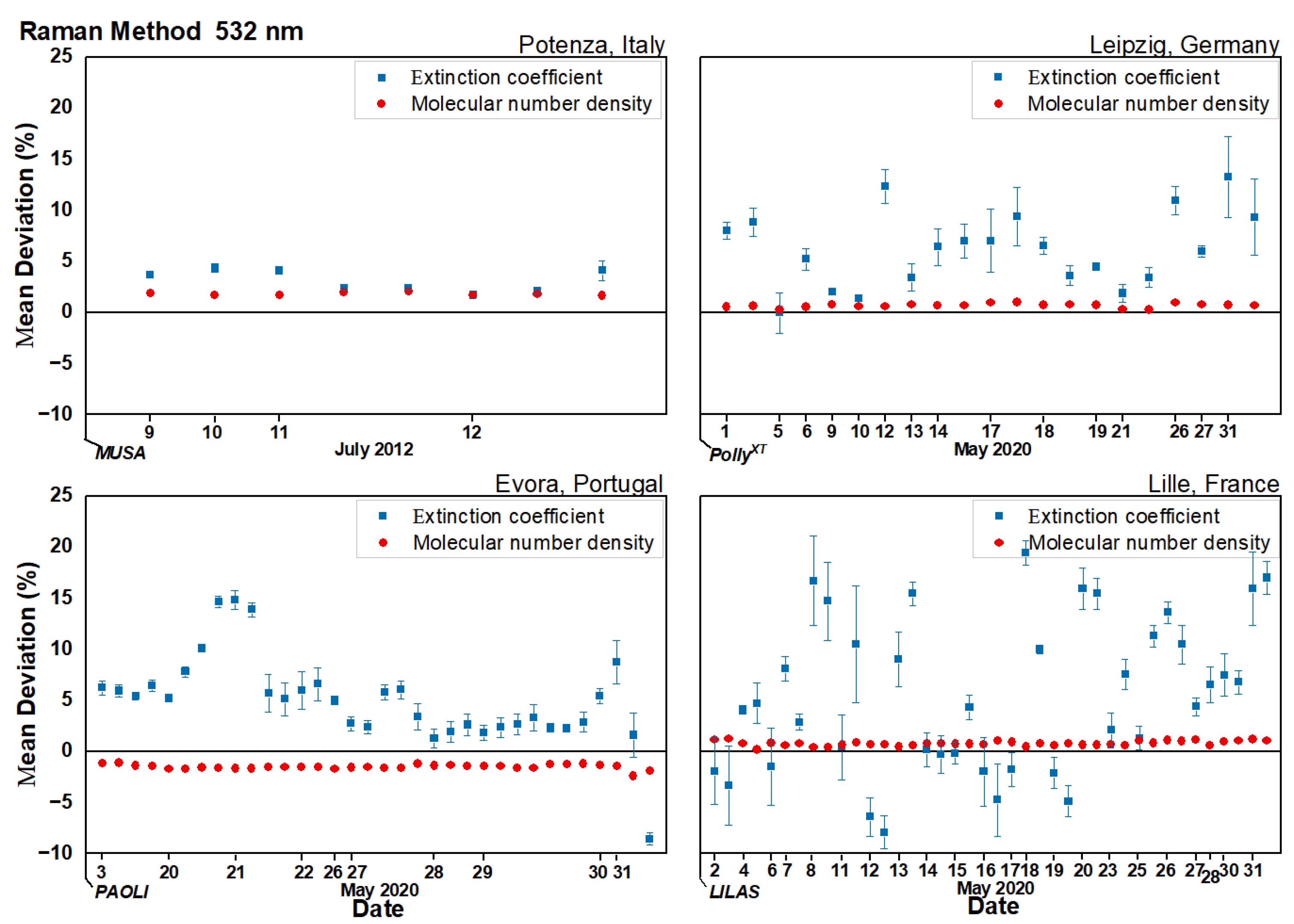
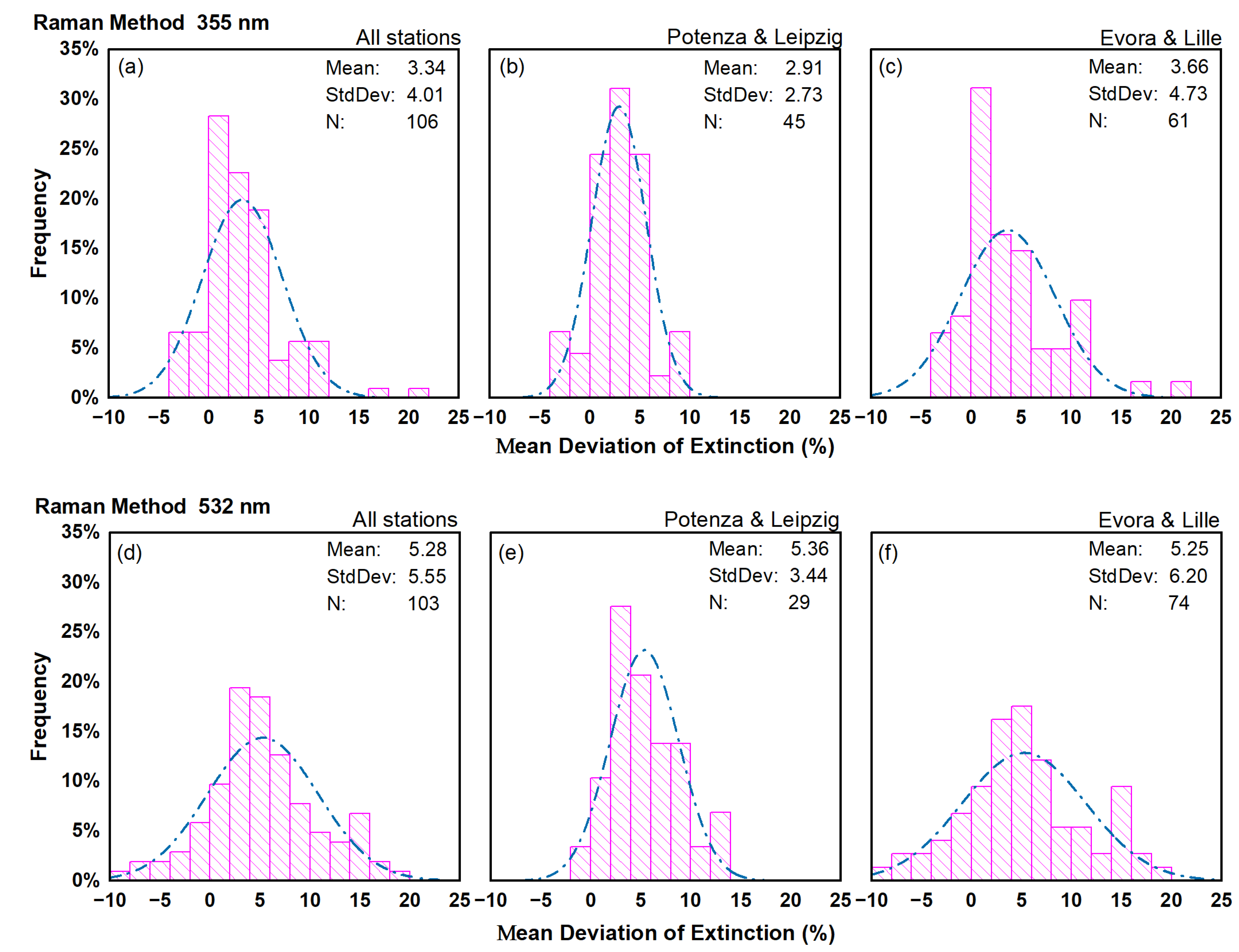
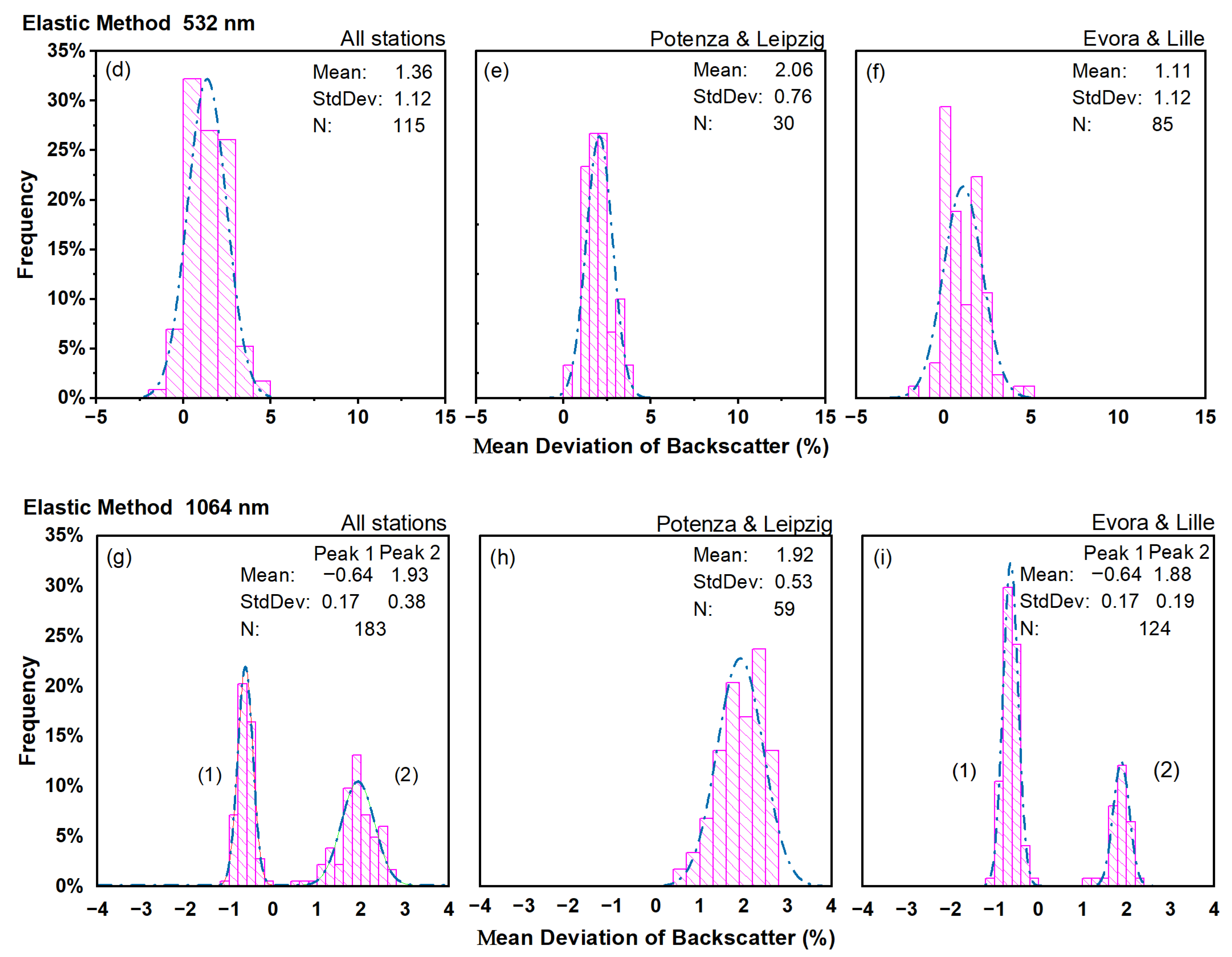
4.1. Deviation of Aerosol Extinction Coefficients

In Figure 1, the mean relative deviations of aerosol extinction at 355 nm for all four stations, are shown. In particular, blue and red dots represent the mean relative deviation of aerosol extinction and atmospheric molecular number density, respectively, when forecast or reanalysis are considered, whereas the deviations are referred to the values calculated with ERA5 from the values calculated with forecast (IFS_ECMWF or GDAS). It is important to underline that the mean relative deviation on aerosol extinction can vary widely and even reaches a maximum value of about 20%, while the corresponding mean relative deviation of molecular number density changes minutely and is always within $\pm 3\%$ no matter whether we are comparing IFS_ECMWF vs. ERA5 or GDAS vs. ERA5.

In Figure 2, the mean relative deviation of extinction and molecular number density at 532 nm for all four stations are shown. The results are very similar to those found for the extinction at 355 nm. The maximum value of the deviation of extinction at 532 nm is around 20%, and the mean deviation for all cases is around 5%. For all cases, the mean relative deviation of molecular number density is always within $\pm 3\%$.

Considering the results in Figure 1 and Figure 2, we can conclude that the use of different atmospheric model data (forecasts and reanalysis) when retrieving aerosol extinction coefficients with the Raman method can lead to large deviations in the results. As we will see, the deviations in molecular number density calculated using pressure and temperature profiles from different atmospheric models are not the main reason for the large deviation of the aerosol extinction coefficient.

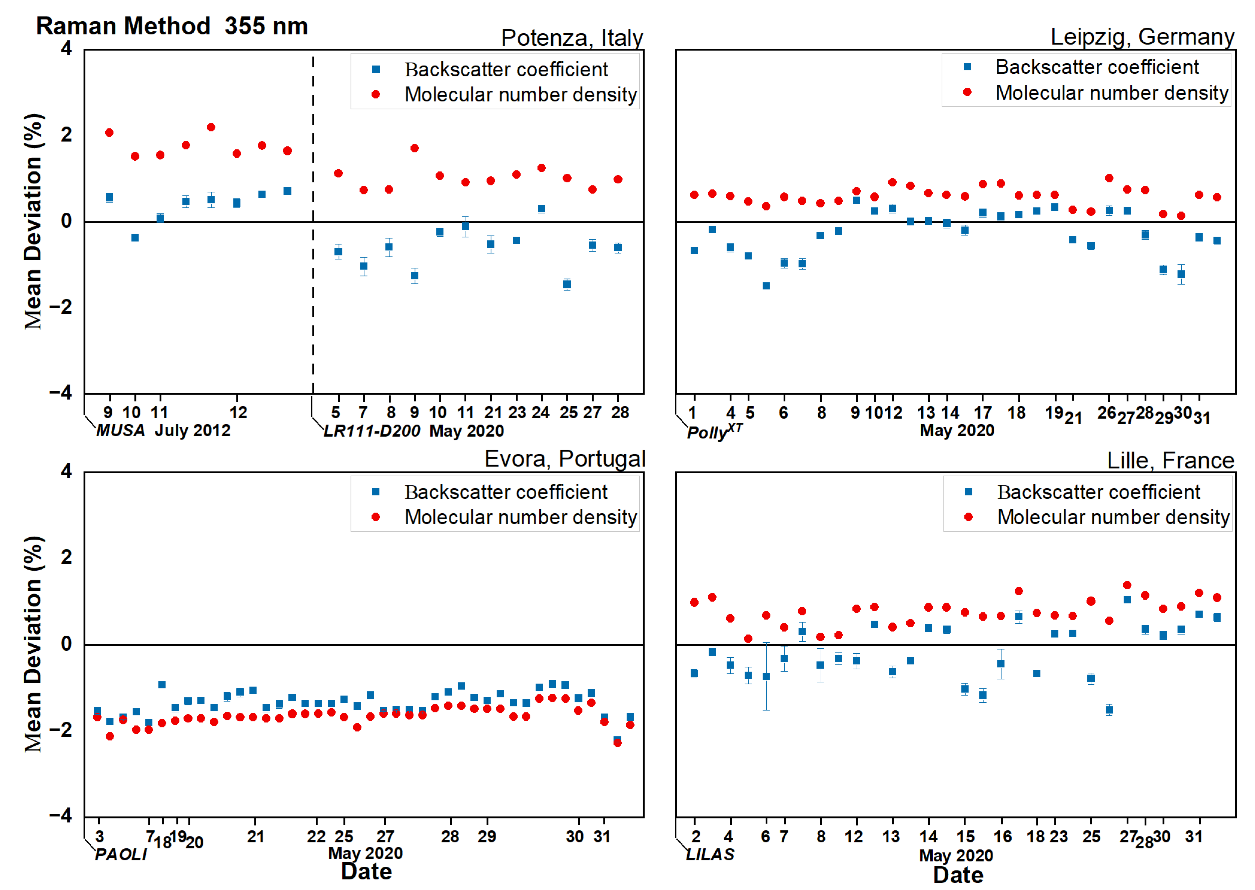
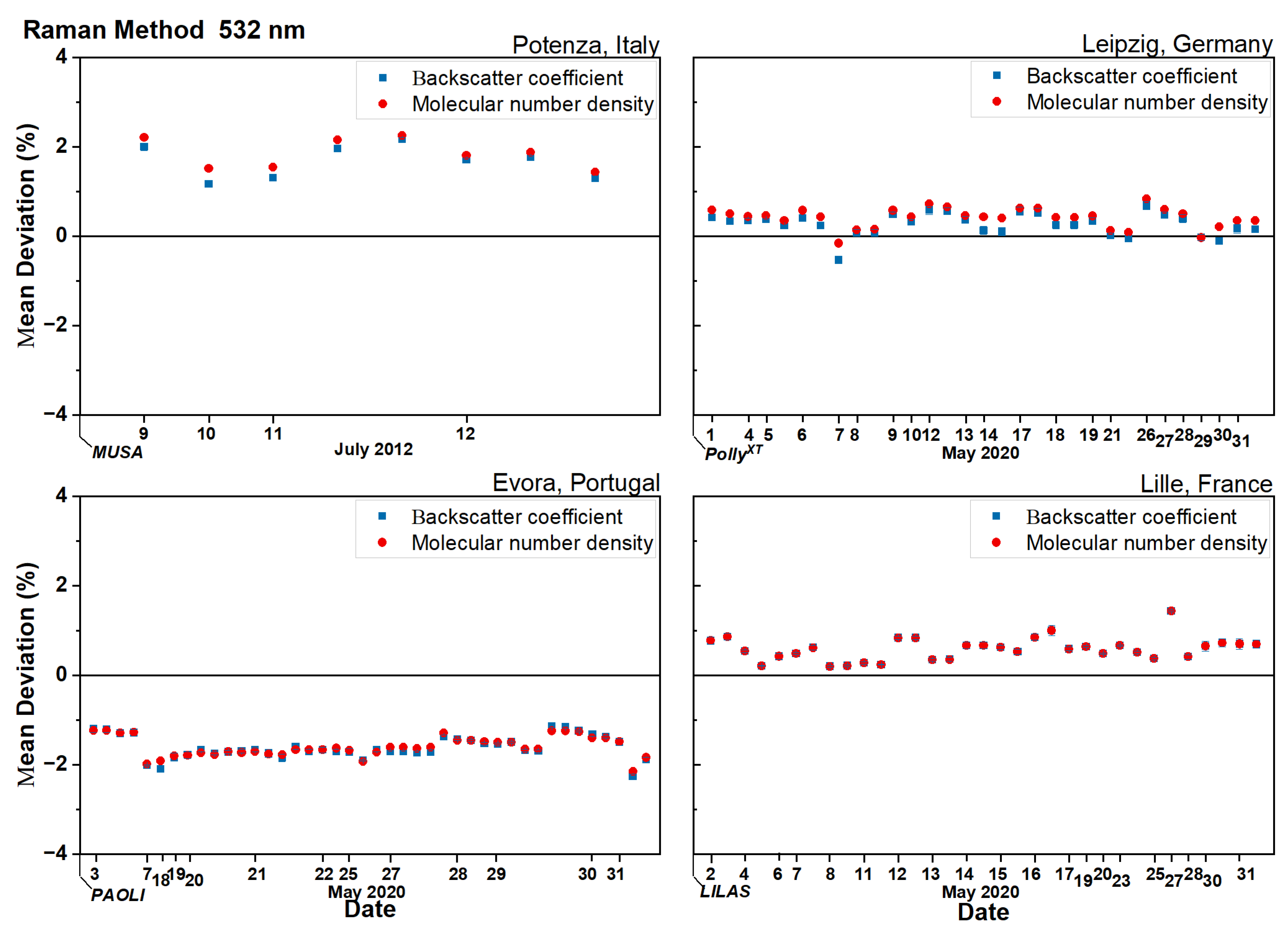
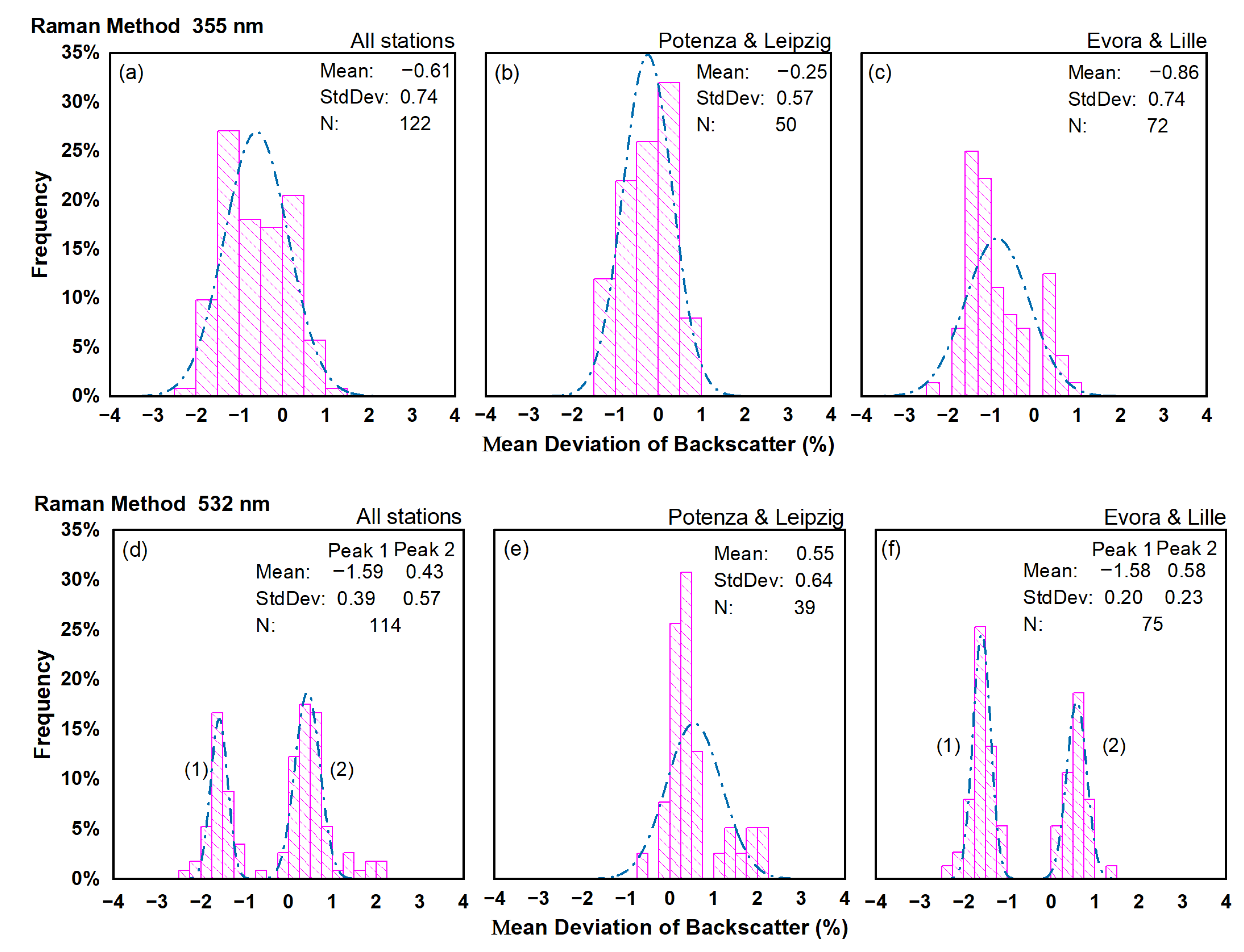
4.2. Deviation of Aerosol Backscatter Coefficients Retrieved with the Raman Method

The mean relative deviation of aerosol backscatter coefficient at 355 nm is shown in Figure 3 for all cases, whereas the deviations are referred to the values calculated with ERA5 from the values calculated with forecast (IFS_ECMWF or GDAS). Blue and red dots represent the mean relative deviation of backscatter and molecular number density, respectively. Same as Figure 3, the results at 532 nm are shown in Figure 4. The aerosol backscatter coefficient is determined from the ratio of the elastic to the inelastic nitrogen Raman signal by using Equation (4).

From Figure 3 and Figure 4 we can find that the mean relative deviation of the Raman backscatter is always within $\pm 3\%$, both at 355 nm and 532 nm. In general, the mean relative deviation of backscatter can follow the mean relative deviation of molecular number density better at 532 nm than at 355 nm. In addition, comparing the results from the extinction and Raman backscatter, the mean relative deviation of the Raman backscatter is smaller and stable, which means that the different atmospheric models can have less influence on the backscatter obtained from the Raman method than the extinction.

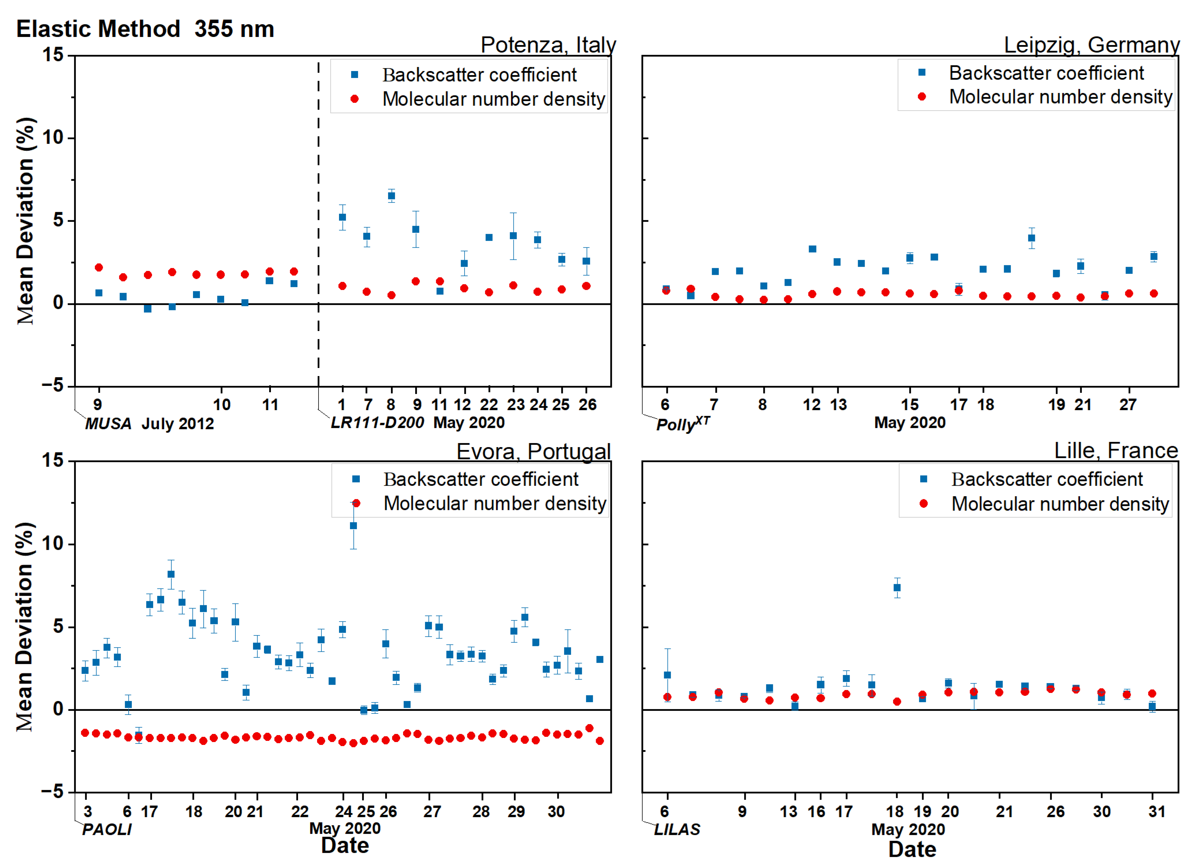
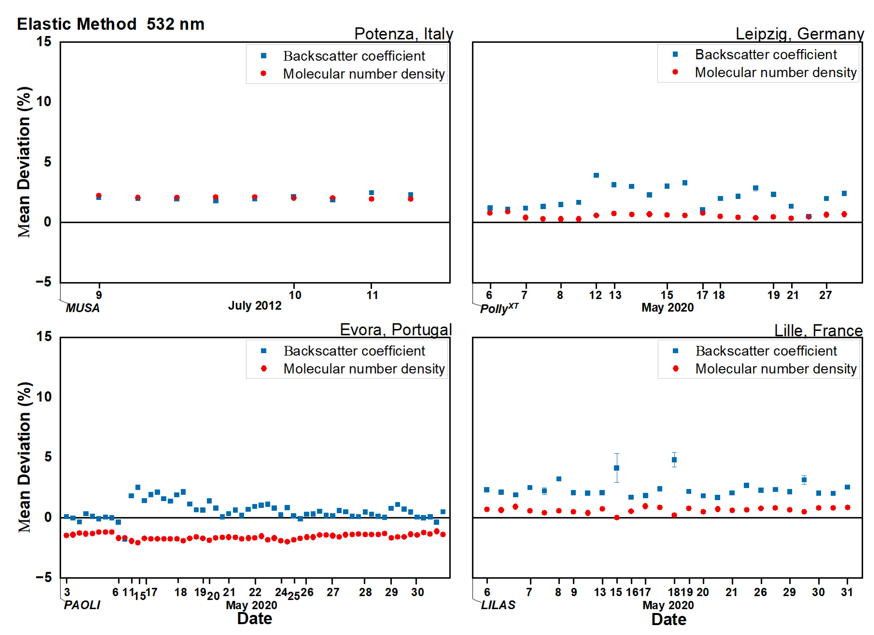
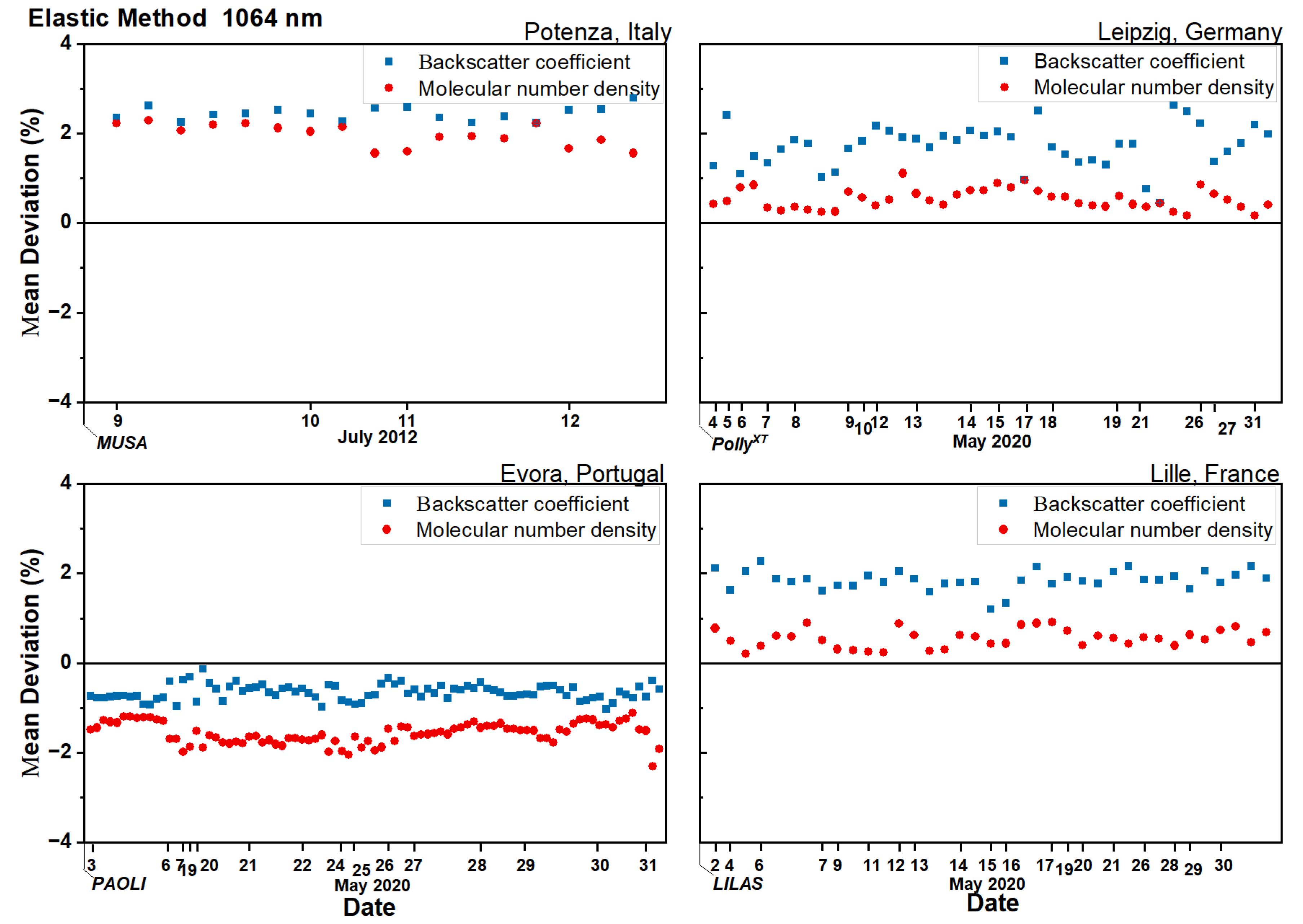
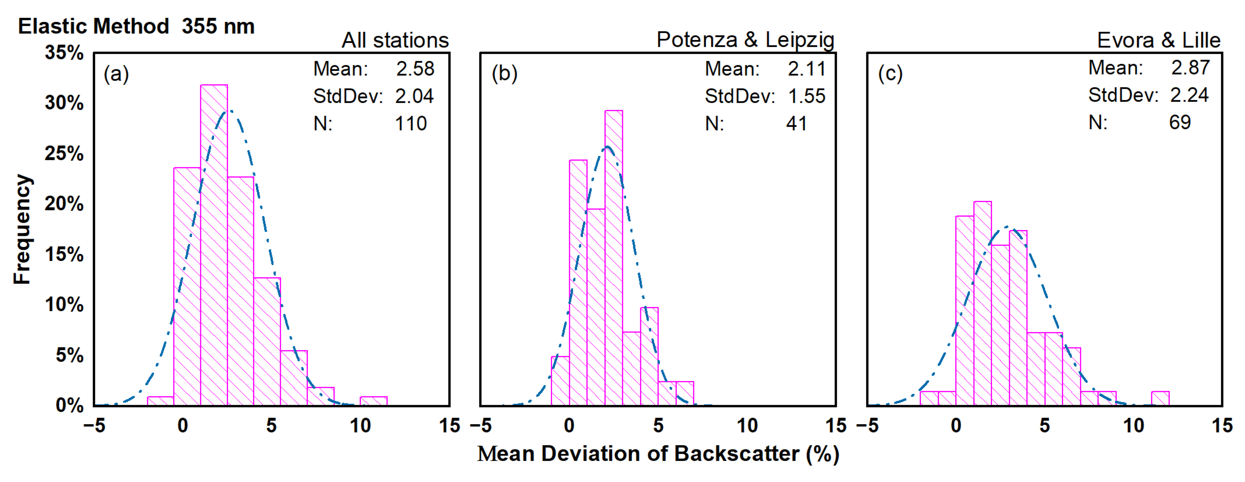
4.3. Deviation of Aerosol Backscatter Coefficient Retrieved with the Elastic Method

It is not always possible to perform Raman lidar measurements. For instance, during the daytime, the solar background can drastically reduce the SNR ratio of the Raman signals, making them too noisy for the retrieval of the aerosol extinction profile. Moreover, the infrared region is quite challenging for detection in photon counting mode and consequently in this spectral region only the elastically backscattered signal is generally measured by the lidar. In all cases in which Raman signals are not available, it is possible to retrieve the aerosol backscatter profile using only elastic-backscatter signals. The most common algorithms used for this type of retrieval are the Klett–Fernald and iterative methods. In this study, we are concerned with investigating the influence of the use of different atmospheric models on the aerosol backscatter coefficient retrieved using the iterative method. We have found that the influence of the usage of different atmospheric models on the aerosol backscatter coefficient retrieved using Klett–Fernald and iterative methods are quite similar, so we refer to the iterative backscatter as elastic backscatter in this paper. In Figure 5, the mean relative deviation of the elastic backscatter coefficient at 355 nm is shown, with the mean relative deviation at 532 nm given in Figure 6 and at 1064 nm in Figure 7.

The mean relative deviation of backscatter at 355 nm, which is represented by blue dots, and the corresponding mean relative deviation of molecular number density, represented by red dots, are shown in Figure 5, where the deviation is expressed as the difference between the values calculated with ERA5 to the values calculated with the forecast (IFS_ECMWF or GDAS). The deviation of molecular number density is within $\pm 3\%$, while the deviation of backscatter is on average 2.6% with a maximum value of about 11%, corresponding to one case of Evora station for which the corresponding mean relative deviation of molecular number density is only −1.7%.

For the elastic backscatter coefficient at 532 nm, the mean relative deviation is within $\pm 5\%$ (see Figure 6). The maximum deviation of backscatter is 4.8%, corresponding to an observation made by the Lille station for which the deviation in the molecular number density is 0.2%.

Finally, the mean relative deviation of backscatter at 1064 nm is shown in Figure 7, both for nighttime and daytime conditions. Differently from the other lidar wavelengths, Raman measurements are not available at 1064 nm in both nighttime and daytime conditions. The deviations of backscatter at 1064 nm for all cases are within $\pm 3\%$, and, if compared with the results at 355 nm and 532 nm, are the smallest.

5. Discussion

5.1. Aerosol Extinction

According to the results shown in Section 4, the deviation from the forecast model to reanalysis data is, in general, larger for the aerosol extinction coefficient obtained from the Raman method, compared to the backscatter coefficient obtained by either the Raman method or the elastic method. Such considerable deviation in aerosol extinction is not correlated with any specific conditions of the atmospheric aerosol load. This can be clearly seen by looking at Figure 8a, showing an almost independent mean relative deviation of extinction with respect to the corresponding aerosol load (expressed in terms of AOD) for all the 106 cases considered at 355 nm.

To understand the reasons for the observed deviations in the aerosol extinction, it should be noted that in Equation (3) there is a term containing the first derivative of the quantity $\ln \left[N_R\left(z\right)/(P_R\left(z\right)z^2\right)]$. This means that the extinction retrieval can be affected not only by absolute differences of the numerical molecular density but also by the difference in terms of the gradient of the profile N_R(z). Consequently, it is possible to observe large deviations in the extinction retrieved from two molecular density profiles very similar in terms of absolute values but different in terms of the corresponding gradients. In Figure 8b, the mean relative deviation of the aerosol extinction at 355 nm is reported as a function of the mean relative deviation of the molecular number density gradient. This gradient has been calculated by applying the same sliding linear fit used to compute the extinction profile. There is an obvious relationship between the mean relative deviation of the molecular number density gradient and the mean relative deviation of extinction. In particular, as expected, the deviations on the extinction profile decrease if the differences in the gradient of molecular number density decrease. As mentioned earlier, the molecular number density is obtained from model pressure and temperature profiles. Typically, the atmospheric temperature can show higher variability in both time and space than the atmospheric pressure. So, in general, it is expected that deviations in the molecular density are mainly due to differences in temperature between forecasts and reanalysis. Figure 8c confirms this hypothesis showing a clear correlation between differences in temperature gradient and the corresponding differences in the molecular density gradients. For example, we report in Figure 9 the temperature profiles (red lines) and temperature gradients (blue lines) obtained from the forecast and the reanalysis corresponding to the two cases in which the deviations in the aerosol extinction shown in Figure 1 are the highest and the lowest. The triangle and round shape represent the data from the GDAS and ERA5 models, respectively. In Figure 9, the region labelled as “comparison area”, representing the data range used to calculate the deviations and the corresponding temperature from different models, are shown. In these two cases, looking at Figure 9a, it is evident that there are large differences in the temperature gradients (which are responsible for the highest deviation in the aerosol extinction), even if the absolute values of the temperature are quite similar. On the other hand, the temperature profiles shown in Figure 9b have similar gradients, but quite different absolute values. Despite this variation in absolute values, the corresponding extinction profiles show the lowest deviation (0.002%). In conclusion, we can say that the temperature gradient used to compute the atmospheric molecular number density can play an important role in aerosol extinction retrieval [22]. In general, forecasts (IFS_ECMWF and GDAS) and reanalysis (ERA5) can provide temperature profiles that locally could have non-negligible differences in gradients. Even if the highest deviation case does not seem to happen often (only 1.9% of the cases considered in this study), it is not possible to exclude a-priori large deviations (20% in this study in the worst case) on aerosol extinction at 355 nm. Furthermore, for the aerosol extinction at 532 nm, we have obtained overall results (not reported here) quite similar to the ones at 355 nm reported in Figure 8b,c. Differently from the extinction at 355 nm, there is a weak dependence of the extinction mean relative deviations on the aerosol load at 532 nm. In particular, high aerosol loads tend to provide a smaller deviation in the extinction at 532 nm. This behavior can be explained considering that usually the nitrogen Raman signal at 607 nm is characterized by a lower SNR with respect to the nitrogen Raman signal at 387 nm. Consequently, the extinction retrieval at 532 nm is less stable in the presence of low aerosol load. In addition, as discussed later, we do not find a clear dependence of the Raman backscatter deviations from the aerosol load, at both 355 nm and 532 nm.

Figure 10 shows the frequency distributions of the mean relative deviation of extinction at 355 nm and 532 nm. To investigate whether there are differences in using IFS_ECMWF and GDAS forecasts, separate comparisons of the two forecasts with the corresponding ERA5 model data have been performed and are provided. As mentioned earlier, the IFS_ECMWF data are used for the Potenza and Leipzig stations, while GDAS data are used for the Evora and Lille stations. Figure 10a reports the frequency distribution of the mean relative deviation of extinction at 355 nm from all 106 cases. The center of the distribution is about 3%, and around 83% of cases are located at the mean relative deviation of the extinction within $\pm 5\%$. The cases in which deviation of extinction is above $\pm$10% are only 8, corresponding to 7.5% of the total cases. Assuming that $\pm 5\%$ is acceptable for the mean relative deviation of extinction, we can conclude that there is a quite high probability (larger than 80%) to be within this limit in retrieving aerosol extinction profile at 355 nm when forecasts (both IFS_ECMWF and GDAS) are used instead of the reanalysis. The frequency distribution of the mean relative deviation of extinction at 532 nm for all four stations is shown in Figure 10d. Here we can see that the center of the distribution is around 5%. Differently from the results at 355 nm, around 60% of the 103 total cases are within the limit of $\pm 5\%$ of mean relative deviations, and there are 19 cases (corresponding to a probability of around 20%), for which the deviation of the extinction is above $\pm 10\%$. This means that, in general, the usage of the forecasts instead of reanalysis is more critical for the retrieval of the aerosol extinction at 532 nm with respect to what we have found for aerosol extinction at 355 nm.

For aerosol extinction at 355 nm, the mean value of the deviation’s distribution is about 3%, regardless of whether IFS_ECMWF or GDAS models are used (see Figure 10b,c). Around 90% of cases show extinction mean relative deviations below $\pm 5\%$, and no cases are found in the large deviation area ($>\pm 10\%$) when IFS_ECMWF model data are considered (Potenza and Leipzig stations). For Evora and Lille stations, for which the GDAS model is used, around 77% of all the 61 cases are within the limit of $\pm 5\%$, and there are 8 cases (around 13%) for which the deviation of extinction is above $\pm 10\%$. In particular, there is only one case for which the mean relative deviation of extinction exceeds 20%.

In Figure 10e,f, the frequency distributions of the mean relative deviation of extinction from two different forecast models at 532 nm are shown. The center of the distributions is about 5%, no matter whether the IFS_ECMWF or the GDAS model is used. Specifically, there is a probability of 62.1% and 56.8% to be within in the acceptable area ($\pm 5\%$) for the IFS_ECMWF or the GDAS model, respectively. As for the large deviation area ($>\pm 10\%$), the probability is 10.3% and 21.6%, respectively.

Based on these results, we can conclude that the usage of IFS_ECMWF provides, in general, the smallest deviations on the extinction retrieval with respect to the case in which ERA5 is considered at both lidar wavelengths. In addition, the standard deviation of the frequency distributions for Evora and Lille stations is higher than the corresponding standard deviation for Potenza and Leipzig stations, both at 355 nm and 532 nm.

Table 4. The mean value of the mean relative deviation of extinction and mean relative deviation of molecular number density and the mean relative deviation of the gradient in molecular number density and mean aerosol load at 355 and 532 nm.

Lidar Name	355 nm				532 nm
	M_DA 1 (%)	M_DNA 2 (%)	M_SNA 3 (%)	M_AOD 4	M_DA (%)	M_DNA (%)	M_SNA (%)	M_AOD
MUSA	2.36	1.85	−1.4	0.175	3.10	1.81	−1.69	0.233
LR111-D200	4.22	1.2	−2.34	0.111	−	−	−	−
PollyXT	2.65	0.71	−2.36	0.133	6.22	0.67	−2.97	0.071
PAOLI	2.34	−1.44	−3.12	0.168	4.99	−1.53	−4.89	0.098
LILAS	4.36	0.85	−2.29	0.194	5.47	0.76	−2.50	0.138
Total	3.34	0.46	−2.41	0.164	5.28	0.07	−3.32	0.118

¹ M_DA: mean value of the mean relative deviation of extinction. ² M_DNA: mean value of the mean relative deviation of molecular number density. ³ M_SNA: mean value of the mean relative deviation of the gradient in molecular number density. ⁴ M_AOD: mean aerosol load.

shows the mean value of the mean relative deviation of extinction, the mean relative deviation of molecular number density and its gradient, and the mean aerosol load for all four stations at two different wavelengths. Combining the values reported in Table 4 with the results shown in Figure 8, it can be seen that the deviation of extinction is mainly determined by deviations in the gradient of the molecular number density (which in turn is caused by differences in the gradient of the atmospheric temperature profile) rather than the mean relative deviation of the molecular number density.

Table 5. Same as Table 4, but for two different forecast models compared with the corresponding reanalysis model.

Model Used	355 nm				532 nm
	M_DA (%)	M_DNA (%)	M_SNA (%)	M_AOD	M_DA (%)	M_DNA (%)	M_SNA (%)	M_AOD
ECMWF/ERA5	2.91	1.01	−2.19	0.136	5.36	0.98	−2.62	0.116
GDAS/ERA5	3.66	0.06	−2.58	0.185	5.25	-0.29	−3.60	0.119

shows the same information provided by Table 4, but from two different forecast models at 355 nm and 532 nm. The larger standard deviation for the frequency distribution obtained for Evora and Lille stations could be an effect of the coarser vertical resolution of the GDAS model with respect to the IFS_ECMWF one. As discussed earlier, the extinction retrieval is sensitive to the temperature vertical gradient, which, in general, is more accurate as the model resolution increases. According to this, concerning the extinction retrieval, it is recommended to choose the model with higher vertical resolution where possible.

5.2. Raman Backscatter

The frequency distribution of the mean relative deviation of Raman backscatter at 355 nm for all stations is shown in Figure 11a. The center of the distribution is around −0.6%, indicating that the usage of forecasts instead of reanalysis introduces quite low deviations in the Raman backscatter retrieval. Moreover, for around 61% of all the cases, the mean relative deviation of the backscatter is within $\pm 1\%$, and only for one case is the deviation above $\pm 2\%$.

The distribution of the deviations characterizing the Raman backscatter retrieval at 532 nm is shown in Figure 11d and looks quite different from the one shown in Figure 11a, with the presence of two different peaks with centers in −1.59% and 0.43%, respectively. The negative centered peak refers to the observations of Evora, where the mean relative deviation of molecular number density obtained from GDAS and ERA5 is negative. For all the other three stations, this deviation is always positive and, consequently, the deviation on the Raman backscatter is positive as well. It should be noted that, differently from the extinction, the Raman backscatter retrieval depends on the absolute value of the molecular number density. This is the reason for which negative deviations of the molecular number density profile are responsible for negative deviations on the retrieved Raman backscatter profile, but they do not affect the sign of the deviations on the retrieved extinction (which are positive in all the cases). Moreover, such difference cannot be due to a general behavior of the GDAS model because GDAS data give positive deviations in molecular number density for the Lille station.

When IFS_ECMWF and GDAS models are considered separately, the center of the distribution at 355 nm is −0.25% and −0.86%, respectively (see Figure 11b,c). The probability of a mean relative deviation of the Raman backscatter between −1% and +1% is 88% and 44%, respectively. Compared to the Potenza and Leipzig stations, the standard deviation shows a higher value for Evora and Lille stations.

As for 532 nm, the frequency distributions show the different shapes reported in Figure 11e,f. For the Potenza and Leipzig stations, the distribution shows one peak centered around 0.55%, with a 79.5% probability of having a mean relative deviation of the backscatter within $\pm 1\%$. For Evora and Lille stations, there are two peaks: one at −1.58% for Evora and another at 0.58% for Lille. Both distributions have almost the same standard deviations.

In general, we can conclude that the usage of forecast in the retrieval of the Raman backscatter produces quite low deviations (well below 3%) with respect to the usage of reanalysis at both 355 nm and 532 nm. Consequently, forecasts (GDAS or IFS_ECMWF) can be used without introducing large uncertainties. In addition, it is possible to infer the presence of two peaks also at 355 nm, but these are not visible because, in this case, they are not resolved. Comparing the results of 532 nm and 355 nm, whether using the IFS_ECMWF or GDAS model, the same deviations in molecular number density seem to introduce slightly larger deviations on Raman backscatter at a longer wavelength.

Table 6. The mean value of the mean relative deviation of the backscatter and mean relative deviation of molecular number density and mean aerosol load at two wavelengths. The backscatter was obtained by the Raman method.

Lidar Name	355 nm			532 nm
	M_DB 1 (%)	M_DNB 2 (%)	M_AOD	M_DB (%)	M_DNB (%)	M_AOD
MUSA	0.38	1.76	0.175	1.67	1.85	0.233
LR111-D200	−0.60	1.03	0.088	−	−	−
PollyXT	−0.28	0.59	0.125	0.26	0.41	0.057
PAOLI	−1.35	−1.66	0.125	−1.62	−1.61	0.084
LILAS	−0.16	0.76	0.218	0.59	0.58	0.144
Total	−0.61	−0.023	0.148	−0.24	−0.18	0.105

¹ M_DB: mean value of the mean relative deviation of backscatter. ² M_DNB: mean value of the mean relative deviation of molecular number density.

shows the mean value of the mean relative deviation of the Raman backscatter and the mean relative deviation of molecular number density and mean aerosol load.

Table 7. Same as Table 6, but for two different forecast models compared with the corresponding reanalysis model.

Model Used	355 nm			532 nm
	M_DB (%)	M_DNB (%)	M_AOD	M_DB (%)	M_DNB (%)	M_AOD
ECMWF/ERA5	−0.25	0.88	0.124	0.55	0.70	0.093
GDAS/ERA5	−0.86	−0.65	0.164	−0.65	−0.64	0.111

shows the same as Table 6 but from two different forecast models. Compared to 355 nm, the mean values of the mean relative deviation of backscatter and the mean relative deviation of molecular number density show higher correlation at 532 nm, no matter whether the IFS_ECMWF or the GDAS model is used.

5.3. Elastic Backscatter

For the backscatter obtained only from elastic signals, the atmospheric aerosol load (expressed in terms of IB) shows a significant influence on the mean deviations, especially for shorter wavelengths. In correspondence to low aerosol load conditions (IB < 0.0015 sr⁻¹), the deviation of elastic backscatter at 355 nm changes from −1.5% to 11%, even if the deviation of the molecular number density profile for the same cases remains almost constant to a quite low value (around −2%). The results of elastic backscatter retrieval at 532 nm and 1064 nm are similar to those obtained for the Raman backscatter retrieval. Most probably this is a consequence of the higher contrast between aerosol and molecular signals at longer wavelengths. Consequently, when the aerosol load is low, the total elastic signal measured at 355 nm is dominated by molecular backscattered signal more than the elastic signals at 532 nm and 1064 nm. In general, this condition makes the retrieval of the elastic backscatter more unstable at shorter wavelengths and, consequently, the influence of aerosol load on the backscatter deviation decreases with the increase of the wavelength, showing the largest effect at 355 nm and the smaller one at 1064 nm.

Figure 12 shows the frequency distributions of the mean relative deviation of elastic backscatter at 355 nm, 532 nm, and 1064 nm. Looking at Figure 12a, for the deviation of elastic backscatter at 355 nm, there are around 92% of cases from all the stations within $\pm 5\%$ and around a 1% probability that the same deviation is above 10%.

The mean relative deviation of elastic backscatter at 532 nm is always within $\pm 5\%$ (see Figure 12d). Moreover, a lower standard deviation of the frequency distribution is obtained with respect to what is found at 355 nm. This is a direct consequence of the higher stability of the elastic backscatter retrieval at longer wavelengths.

The frequency distribution of the mean relative deviation of elastic backscatter at 1064 nm is different from the ones at the other two wavelengths as two peaks centered at –0.64% and 1.93% are clearly visible in Figure 12g. The shape of the distribution in Figure 12g is similar to the one reported in Figure 11d for the Raman backscatter at 532 nm. Additionally, in this case the negative peak refers to the Evora observations where there is a negative deviation in the molecular number density calculated out of GDAS and ERA5 model data (see Figure 7). Furthermore, the mean relative deviation of backscatter at 1064 nm is not so sensitive to the aerosol load. The complex influence of these two factors causes the frequency distribution at 1064, showing the two peaks reported in Figure 12g.

At 355 nm, the distribution is centered at 2.11% when the IFS_ECMWF model is used and at 2.87% when the GDAS model is used. The probability to have elastic backscatter deviations within $\pm 5\%$ is about 95% and 83% for IFS_ECMWF and GDAS, respectively (see Figure 12b,c).

At 532 nm, there is a 100% probability to have $\pm 5\%$ elastic backscatter deviations regardless of the IFS_ECMWF or GDAS model is used (see Figure 12e,f).

Finally, at 1064 nm, different distributions are obtained if IFS_ECMWF or GDAS model data are considered. The distribution obtained for Potenza and Leipzig (IFS_ECMWF) is shown in Figure 12h. It is centered at 1.92%, and in all cases the deviations of backscatter are within $\pm 3\%$. Different characteristics are found for the distribution corresponding to Evora and Lille stations (GDAS), where two separate peaks are found (see Figure 12i), which are clearly resolved at 1064 nm, partially at 532 nm, and not resolved at 355 nm This result is quite similar to what we have found for the Raman backscatter deviations at 532 nm (see, Figure 11f). The mean value corresponding to the two peaks is −0.64% (corresponding to Evora station) and 1.88% (corresponding to Lille station).

If we make a comparison among the frequency distributions at the three wavelengths, we can find that the mean deviation of elastic backscatter and standard deviation of frequency distributions both decrease with the wavelength increase for the Potenza and Leipzig stations. Combined with the effect of aerosol load on the results, we can conclude that the mean relative deviation of the elastic backscatter at shorter wavelengths is more sensitive to the aerosol load, producing a more unstable and higher deviation result.

In general, the distribution obtained for Evora and Lille observations has a larger standard deviation with respect to the corresponding ones obtained for Potenza and Leipzig stations at all wavelengths. This is because only for Evora did we observe a negative mean deviation of the molecular density between GDAS and ERA5 model data.

Table 8. The mean value of the mean relative deviation of backscatter and the mean relative deviation of molecular number density and mean aerosol load at three wavelengths. The backscatter was obtained by the elastic method.

Lidar Name	355 nm			532 nm			1064 nm
	M_DB (%)	M_DNB (%)	M_IB 1 (sr−1)	M_DB (%)	M_DNB (%)	M_IB (sr−1)	M_DB (%)	M_DNB (%)	M_IB (sr−1)
MUSA	0.44	1.83	0.0055	2.06	2.05	0.0044	2.44	1.97	0.0027
LR111-D200	3.70	0.94	0.0023	−	−	−	−	−	−
PollyXT	1.99	0.53	0.0028	2.06	0.54	0.0015	1.71	0.53	0.0008
PAOLI	3.44	−1.67	0.0023	0.55	−1.59	0.0025	−0.65	−1.57	0.0013
LILAS	1.45	0.91	0.0077	2.38	0.61	0.0024	1.85	0.55	0.0010
Total	2.58	−0.23	0.0036	1.36	−0.42	0.0025	0.68	−0.33	0.0012

¹ M_IB: mean aerosol load.

shows the mean value of the mean relative deviation of elastic backscatter, the mean relative deviation of molecular number density and the mean aerosol load. The mean value of the mean relative deviation of elastic backscatter is always within $\pm 4\%$ for all three wavelengths, with the deviation of molecular number density within $\pm 3\%$. The same as in Table 8, but from two different forecast models, is shown in

Table 9. Same as Table 8, but for two different forecast models compared with the corresponding reanalysis model.

Model Used	355 nm			532 nm			1064 nm
	M_DB (%)	M_DNB (%)	M_IB (sr−1)	M_DB (%)	M_DNB (%)	M_IB (sr−1)	M_DB (%)	M_DNB (%)	M_IB (sr−1)
ECMWF/ERA5	2.11	0.93	0.0033	2.06	0.99	0.0024	1.92	0.94	0.0013
GDAS/ERA5	2.87	−0.93	0.0039	1.11	−0.92	0.0025	0.09	−0.93	0.0012

.

6. Conclusions

To evaluate the effect of different atmospheric models on the final aerosol optical products (backscatter and extinction coefficients), the data from four European Aerosol Research Lidar Network (EARLINET) stations, measured during two intensive campaigns, have been considered. The impact of different atmospheric models on the lidar retrievals of aerosol extinction and Raman/elastic backscatter has been assessed by applying the same retrieval algorithms on the same input data and changing only the model data (forecasts or reanalysis) used to compute the atmospheric molecular density vertical profiles from temperature and pressure profiles. The forecast models used here were the Integrated Forecasting System operated by the European Centre for Medium-Range Weather Forecasts (IFS_ECMWF) for Potenza and Leipzig stations and the Global Data Assimilation System (GDAS) for Evora and Lille stations. The fifth-generation ECMWF atmospheric reanalysis system (ERA5) has been considered for all measurement sites. The results are summarized by the following points.

(a)

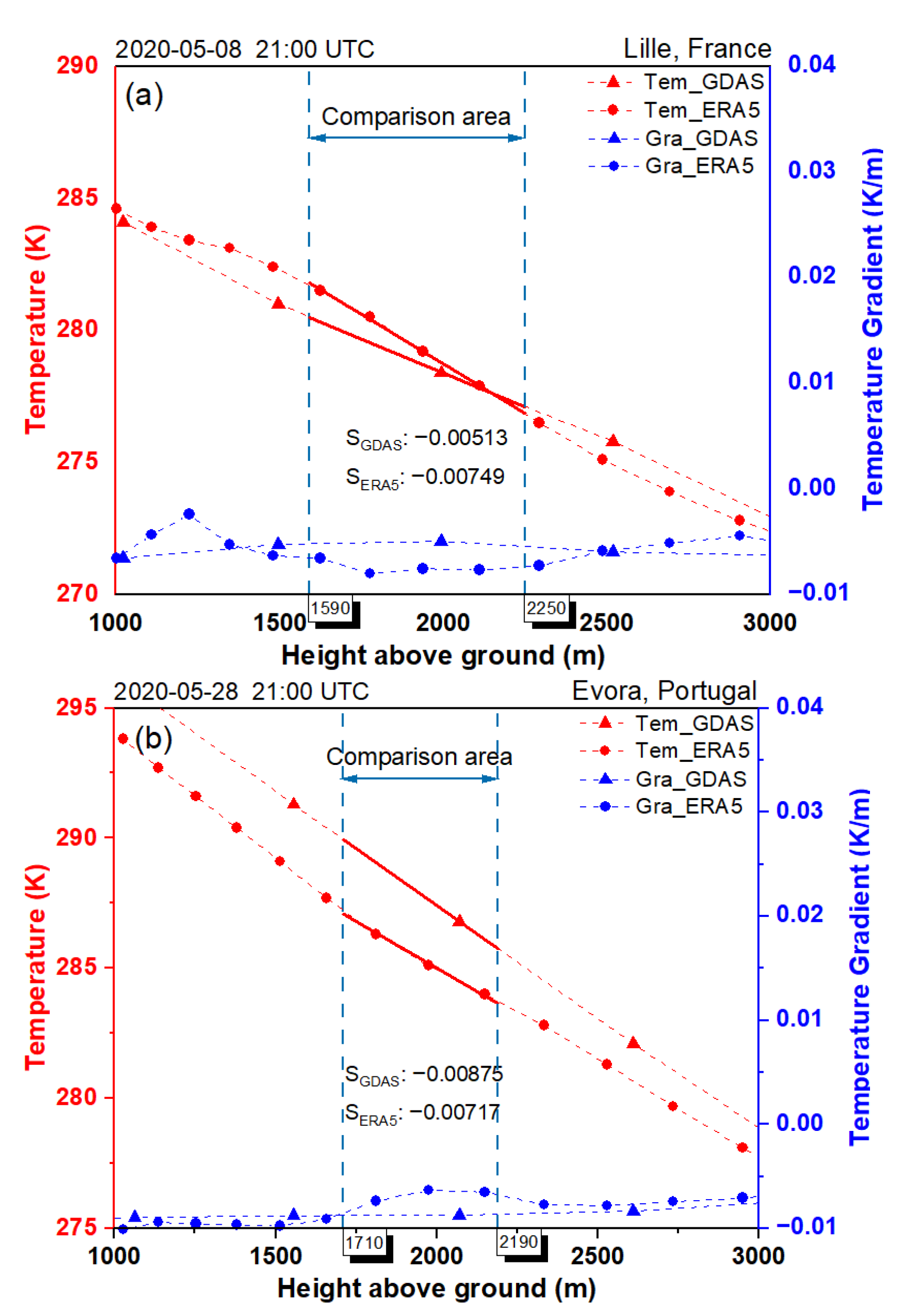
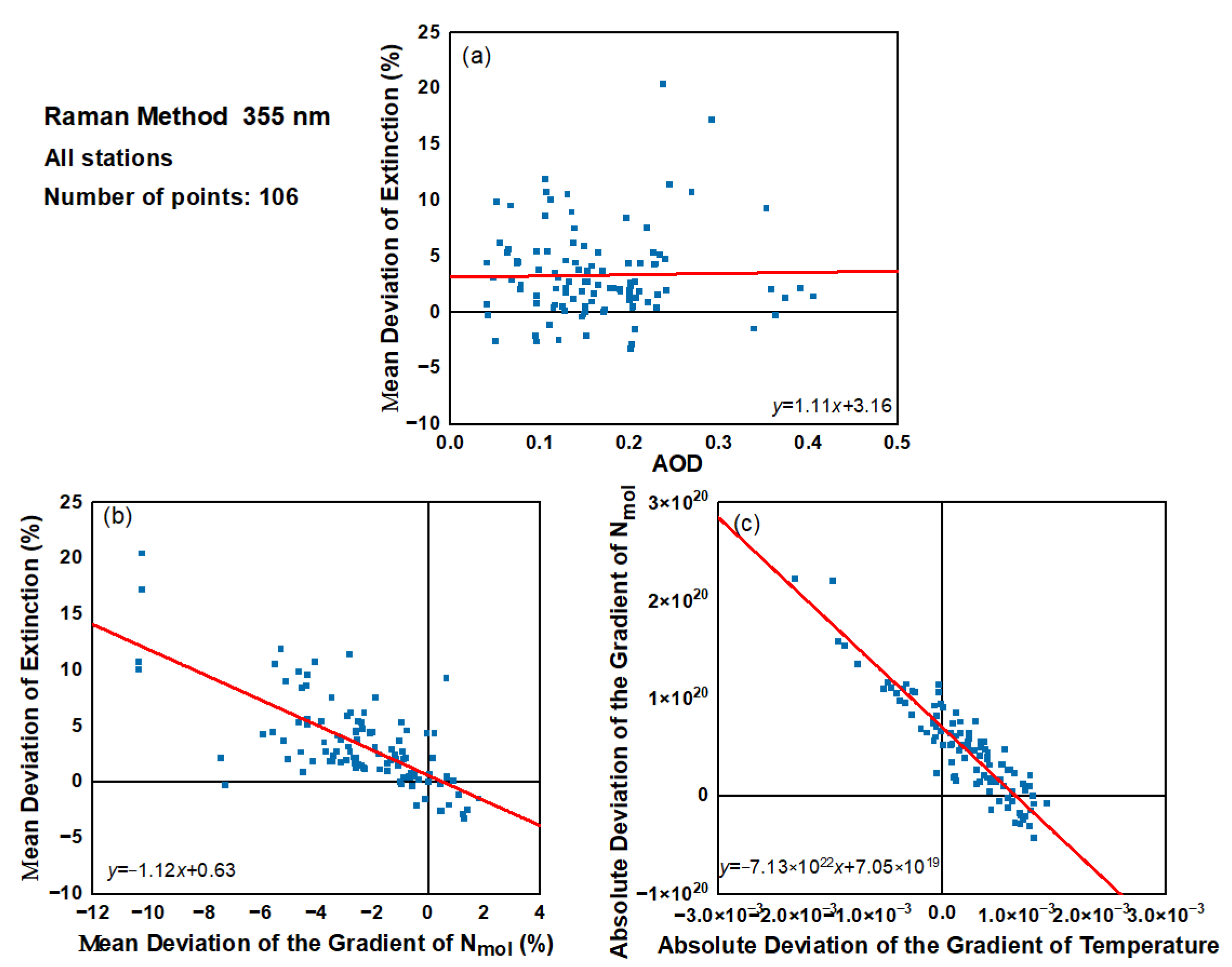
The use of different model data may have a non-negligible influence on the lidar aerosol extinction retrieval, due mainly to the differences in the gradient of the molecular density profile. This arises from the differences in the vertical temperature gradients, provided by forecast models and reanalysis, instead of the absolute deviation of the molecular number density, which, in general, is quite similar in both forecasts and reanalysis. Even if the average deviation for all cases is small (3.34% at 355 nm and 5.28% at 532 nm), there are a few cases displaying larger deviations. Therefore, the use of a forecast rather than reanalysis in the aerosol extinction retrieval should be carefully considered as it is not possible to exclude high deviations, although this was found very rarely in this study.

(b)

The use of forecasts and reanalysis has less influence on the retrieval of the backscatter profiles using both Raman and elastic methods. The quite low deviations found for the aerosol backscatter retrieval suggest that, in general, the forecast model can be used to obtain results with high confidence, especially for the Raman method, which shows a lower deviation (well below $\pm 3\%$).

(c)

The atmosphere aerosol load can affect the deviation of extinction and backscatter, independently of the retrieval algorithm (Raman or elastic). Lower aerosol load conditions will lead to larger deviations in the aerosol products (extinction and backscatter), as also reported in the literature [21,44]. Therefore, under low aerosol load and particularly for the aerosol backscatter retrieved with the elastic method, the usage of the forecast model could introduce not always negligible discrepancies.

(d)

According to our study, the use of the IFS_ECMWF model provides, on average, lower deviations (compared to ERA5) in aerosol extinction retrieval than using GDAS. For the aerosol backscatter retrieval, the deviations are almost the same independent of the forecast model, but a larger standard deviation for the frequency distribution of the mean deviation is observed when GDAS is considered.

Finally, we should note that near-real-time observations are very important for several crucial topics such as real-time monitoring of extreme atmospheric events (volcanic eruptions, forest fires, severe dust intrusions), meteorology studies, and implementation of atmospheric early warning systems. Although reanalysis data (ERA5) is considered to be one of the most accurate and reliable sources of the atmospheric parameters needed as input for lidar retrieval methods at global scale, it is not available in near-real-time. Therefore, forecast models represent the best substitute even if, as shown in this study, there may be non-negligible discrepancies in some cases. A good compromise would be to use the forecast to deliver lidar products in near-real-time and, as soon as the re-analyses are made available, reprocess these products, especially those containing aerosol extinction profiles. Further, the results of this study are also very valuable for space-borne lidars, which use the forecast model data along the track to derive the aerosol properties in near-real-time, such as in ADM-Aeolus and EarthCARE missions.

References

1. Boucher, O.; Randall, D.; Artaxo, P.; Bretherton, C.; Feingold, G.; Forster, P.; Kerminen, V.-M.; Kondo, Y.; Liao, H.; Lohmann, U.; et al. Clouds and Aerosols. In Climate Change 2013: The Physical Science Basis. Contribution of Working Group I to the Fifth Assessment Report of the Intergovernmental Panel on Climate Change; Stocker, T.F., Qin, D., Plattner, G.-K., Tignor, M., Allen, S.K., Boschung, J., Eds.; Cambridge University Press: Cambridge, UK; New York, NY, USA, 2013; pp. 571–658. [Google Scholar] [CrossRef]
2. Ackerman, S.A.; Chung, H. Radiative Effects of Airborne Dust on Regional Energy Budgets at the Top of the Atmosphere. J. Appl. Meteo. Climatol. 1992, 31, 223–233. [Google Scholar] [CrossRef] [Green Version]
3. Ellison, G.B.; Tuck, A.F.; Vaida, V. Atmospheric processing of organic aerosols. J. Geophys. Res. Atmos. 1999, 104, 11633–11641. [Google Scholar] [CrossRef]
4. Izhovkina, N.I.; Artekha, S.N.; Erokhin, N.S.; Mikhailovskaya, L.A. Aerosol, Plasma Vortices and Atmospheric Processes. Izv. Atmos. Ocean. Phys. 2019, 54, 1513–1524. [Google Scholar] [CrossRef]
5. Lelieveld, J.; Evans, J.S.; Fnais, M.; Giannadaki, D.; Pozzer, A. The contribution of outdoor air pollution sources to premature mortality on a global scale. Nature 2015, 525, 367–371. [Google Scholar] [CrossRef] [PubMed]
6. Contini, D.; Lin, Y.-H.; Hänninen, O.; Viana, M. Contribution of Aerosol Sources to Health Impacts. Atmosphere 2021, 12, 730. [Google Scholar] [CrossRef]
7. Chen, Y.-C.; Wang, S.-H.; Min, Q.; Lu, S.; Lin, P.-L.; Lin, N.-H.; Chung, K.-S.; Joseph, E. Aerosol impacts on warm-cloud microphysics and drizzle in a moderately polluted environment. Atmos. Chem. Phys. 2021, 21, 4487–4502. [Google Scholar] [CrossRef]
8. Via, M.; Minguillón, M.C.; Reche, C.; Querol, X.; Alastuey, A. Increase in secondary organic aerosol in an urban environment. Atoms. Chem. Phys. 2021, 21, 8323–8339. [Google Scholar] [CrossRef]
9. Gultepe, I.; Sharman, R.; Williams, P.D.; Zhou, B.; Ellrod, G.; Minnis, P.; Trier, S.; Griffin, S.; Yum, S.S.; Gharabaghi, B.; et al. A Review of High Impact Weather for Aviation Meteorology. Pure Appl. Geophys. 2019, 176, 1869–1921. [Google Scholar] [CrossRef]
10. Burton, S.P.; Ferrare, R.A.; Vaughan, M.A.; Omar, A.H.; Rogers, R.R.; Hostetler, C.A.; Hair, J.W. Aerosol classification from airborne HSRL and comparisons with the CALIPSO vertical feature mask. Atmos. Meas. Tech. 2013, 6, 1397–1412. [Google Scholar] [CrossRef] [Green Version]
11. Papagiannopoulos, N.; Mona, L.; Amodeo, A.; D’Amico, G.; Gumà Claramunt, P.; Pappalardo, G.; Alados-Arboledas, L.; Guerrero-Rascado, J.L.; Amiridis, V.; Kokkalis, P.; et al. An automatic observation-based aerosol typing method for earlinet. Atmos. Chem. Phys. 2018, 18, 15879–15901. [Google Scholar] [CrossRef] [Green Version]
12. Pappalardo, G.; Amodeo, A.; Apituley, A.; Comeron, A.; Freudenthaler, V.; Linné, H.; Ansmann, A.; Bösenberg, J.; D’Amico, G.; Mattis, I.; et al. EARLINET: Towards an advanced sustainable European aerosol lidar network. Atmos. Meas. Tech. 2014, 7, 2389–2409. [Google Scholar] [CrossRef] [Green Version]
13. Pal, S.; Behrendt, A.; Wulfmeyer, V. Elastic-backscatter-lidar-based characterization of the convective boundary layer and investigation of related statistics. Ann. Geophys. 2010, 28, 825–847. [Google Scholar] [CrossRef] [Green Version]
14. Fernald, F.G.; Herman, B.M.; Reagan, J.A. Determination of Aerosol Height Distributions by Lidar. J. Appl. Meteorol. Climatol. 1972, 11, 482–489. [Google Scholar] [CrossRef] [Green Version]
15. Fernald, F.G. Analysis of atmospheric lidar observations: Some comments. Appl. Opt. 1984, 23, 652–653. [Google Scholar] [CrossRef] [PubMed]
16. Klett, J.D. Stable analytical inversion solution for processing lidar returns. Appl. Opt. 1981, 20, 211–220. [Google Scholar] [CrossRef] [Green Version]
17. Klett, J.D. Lidar inversion with variable backscatter/extinction ratios. Appl. Opt. 1985, 24, 1638–1643. [Google Scholar] [CrossRef]
18. Di Girolamo, P.; Ambrico, P.F.; Amodeo, A.; Boselli, A.; Pappalardo, G.; Spinelli, N. Aerosol observations by lidar in the nocturnal boundary layer. Appl. Opt. 1999, 38, 4585–4595. [Google Scholar] [CrossRef]
19. Masci, F. Algorithms for the inversion of lidar signals: Rayleigh-Mie measurements in the stratosphere. Ann. Geophys. 1999, 42, 71–83. [Google Scholar] [CrossRef]
20. Sasano, Y.; Browell, E.V.; Ismail, S. Error caused by using a constant extinction/backscattering ratio in the lidar solution. Appl. Opt. 1985, 24, 3929–3932. [Google Scholar] [CrossRef]
21. Ansmann, A.; Riebesell, M.; Weitkamp, C. Measurement of atmospheric aerosol extinction profiles with a Raman lidar. Opt. Lett. 1990, 15, 746–748. [Google Scholar] [CrossRef]
22. Ansmann, A.; Wandinger, U.; Riebesell, M.; Weitkamp, C.; Michaelis, W. Independent measurement of extinction and backscatter profiles in cirrus clouds by using a combined Raman elastic-backscatter lidar. Appl. Opt. 1992, 31, 7113–7131. [Google Scholar] [CrossRef] [PubMed]
23. Ferrare, R.A.; Turner, D.D.; Brasseur, L.H.; Feltz, W.F.; Dubovik, O.; Tooman, T.P. Raman lidar measurements of the aerosol extinction-to-backscatter ratio over the Southern Great Plains. J. Geophys. Res. Atmos. 2001, 106, 20333–20347. [Google Scholar] [CrossRef] [Green Version]
24. Whiteman, D.N.; Melfi, S.H.; Ferrare, R.A. Raman lidar system for the measurement of water vapor and aerosols in the Earth’s atmosphere. Appl. Opt. 1992, 31, 3068–3082. [Google Scholar] [CrossRef] [PubMed]
25. Amodeo, A.; Bösenberg, J.; Ansmann, A.; Balis, D.; Böckmann, C.; Chaikovsky, A.; Comeron, A.; Mitev, V.; Papayannis, A.; Pappalardo, G.; et al. EARLINET: The European Aerosol Lidar Network. Opt. Pur. Apl. 2006, 39, 1–10. Available online: https://dialnet.unirioja.es/servlet/articulo?codigo=6817905 (accessed on 9 May 2022).
26. Sicard, M.; D’Amico, G.; Comerón, A.; Mona, L.; Alados-Arboledas, L.; Amodeo, A.; Baars, H.; Baldasano, J.M.; Belegante, L.; Binietoglou, I.; et al. EARLINET: Potential operationality of a research network. Atmos. Meas. Tech. 2015, 8, 4587–4613. [Google Scholar] [CrossRef] [Green Version]
27. Matthais, V.; Freudenthaler, V.; Amodeo, A.; Balin, I.; Balis, D.; Bosenberg, J.; Chaikovsky, A.; Chourdakis, G.; Comeron, A.; Delaval, A.; et al. Aerosol lidar intercomparison in the framework of the EARLINET project. 1. Instruments. Appl. Opt. 2004, 43, 961–976. [Google Scholar] [CrossRef] [PubMed]
28. Bockmann, C.; Wandinger, U.; Ansmann, A.; Bosenberg, J.; Amiridis, V.; Boselli, A.; Delaval, A.; Tomasi, F.D.; Frioud, M.; Grigorov, I.V.; et al. Aerosol lidar intercomparison in the framework of the EARLINET project. 2. Aerosol backscatter algorithms. Appl. Opt. 2004, 43, 977–989. [Google Scholar] [CrossRef]
29. Pappalardo, G.; Amodel, A.; Pandolfi, M.; Wandinger, U.; Ansmann, A.; Bösenberg, J.; Matthias, V.; Amiridis, V.; De Tomasi, F.; Frioud, M.; et al. Aerosol lidar intercomparison in the framework of the EARLINET project. 3. Raman lidar algorithm for aerosol extinction, backscatter, and lidar ratio. Appl. Opt. 2004, 43, 5370–5385. [Google Scholar] [CrossRef]
30. Wandinger, U.; Freudenthaler, V.; Baars, H.; Amodeo, A.; Engelmann, R.; Mattis, I.; Groß, S.; Pappalardo, G.; Giunta, A.; D’Amico, G.; et al. EARLINET instrument intercomparison campaigns: Overview on strategy and results. Atmos. Meas. Tech. 2016, 9, 1001–1023. [Google Scholar] [CrossRef] [Green Version]
31. D’Amico, G.; Amodeo, A.; Mattis, I.; Freudenthaler, V.; Pappalardo, G. EARLINET Single Calculus Chain—Technical—Part 1: Pre-processing of raw lidar data. Atmos. Meas. Tech. 2016, 9, 491–507. [Google Scholar] [CrossRef] [Green Version]
32. Mattis, I.; D’Amico, G.; Baars, H.; Amodeo, A.; Madonna, F.; Iarlori, M. EARLINET Single Calculus Chain—Technical—Part 2: Calculation of optical products. Atmos. Meas. Tech. 2016, 9, 3009–3029. [Google Scholar] [CrossRef] [Green Version]
33. Wandinger, U.; Nicolae, D.; Pappalardo, G.; Mona, L.; Comerón, A. ACTRIS and its Aerosol Remote Sensing Component. EPJ Web Conf. 2020, 237, 05003. [Google Scholar] [CrossRef]
34. D’Amico, G.; Amodeo, A.; Baars, H.; Binietoglou, I.; Freudenthaler, V.; Mattis, I.; Wandinger, U.; Pappalardo, G. EARLINET Single Calculus Chain—Overview on methodology and strategy. Atmos. Meas. Tech. 2015, 8, 4891–4916. [Google Scholar] [CrossRef] [Green Version]
35. Madonna, F.; Summa, D.; Di Girolamo, P.; Marra, F.; Wang, Y.; Rosoldi, M. Assessment of Trends and Uncertainties in the Atmospheric Boundary Layer Height Estimated Using Radiosounding Observations over Europe. Atmosphere 2021, 12, 301. [Google Scholar] [CrossRef]
36. Hersbach, H.; Bell, B.; Berrisford, P.; Hirahara, S.; Horányi, A.; Muñoz-Sabater, J.; Nicolas, J.; Peubey, C.; Radu, R.; Schepers, D.; et al. The ERA5 global reanalysis. Q. J. R. Meteoeol. Soc. 2020, 146, 1999–2049. [Google Scholar] [CrossRef]
37. Rémy, S.; Kipling, Z.; Flemming, J.; Boucher, O.; Nabat, P.; Michou, M.; Bozzo, A.; Ades, M.; Huijnen, V.; Benedetti, A.; et al. Description and evaluation of the tropospheric aerosol scheme in the European Centre for Medium-Range Weather Forecasts (ECMWF) Integrated Forecasting System (IFS-AER, cycle 45R1). Geosci. Model Dev. 2019, 12, 4627–4659. [Google Scholar] [CrossRef] [Green Version]
38. Strube, C.; Preusse, P.; Ern, M.; Riese, M. Propagation paths and source distributions of resolved gravity waves in ECMWF-IFS analysis fields around the southern polar night jet. Atmos. Chem. Phys. 2021, 21, 18641–18668. [Google Scholar] [CrossRef]
39. Flemming, J.; Huijnen, V.; Arteta, J.; Bechtold, P.; Beljaars, A.; Blechschmidt, A.M.; Diamantakis, M.; Engelen, R.J.; Gaudel, A.; Inness, A.; et al. Tropospheric chemistry in the Integrated Forecasting System of ECMWF. Geosci. Model Dev. 2015, 8, 975–1003. [Google Scholar] [CrossRef] [Green Version]
40. Abreu, P.; Aglietta, M.; Ahlers, M.; Ahn, E.J.; Albuquerque, I.F.M.; Allard, D.; Allekotte, I.; Allen, J.; Allison, P.; Almela, A.; et al. Description of atmospheric conditions at the Pierre Auger Observatory using the Global Data Assimilation System (GDAS). Astropart. Phys. 2012, 35, 591–607. [Google Scholar] [CrossRef] [Green Version]
41. Illingworth, A.J.; Hogan, R.J.; O’Connor, E.J.; Bouniol, D.; Delanoë, J.; Pelon, J.; Protat, A.; Brooks, M.E.; Gaussiat, N.; Wilson, D.R.; et al. Cloudnet. Bull. Am. Meteorol. Soc. 2007, 88, 883–898. [Google Scholar] [CrossRef] [Green Version]
42. Cooney, J.; Orr, J.; Tomasetti, C. Measurements Separating the Gaseous and Aerosol Components of Laser Atmospheric Backscatter. Nature 1969, 224, 1098–1099. [Google Scholar] [CrossRef]
43. Melfi, S.H. Remote Measurements of the Atmosphere Using Raman Scattering. Appl. Opt. 1972, 11, 1605–1610. [Google Scholar] [CrossRef] [PubMed]
44. Whiteman, D.N. Examination of the traditional Raman lidar technique. I. Evaluating the temperature-dependent lidar equations. Appl. Opt. 2003, 42, 2571–2592. [Google Scholar] [CrossRef] [PubMed]
Figure 1. Mean relative deviations of extinction at 355 nm for the four stations, where the deviation refers to the difference between the values calculated with ERA5 to the values calculated with the forecast (IFS_ECMWF or GDAS). Blue and red dots represent the mean relative deviation of aerosol extinction and molecular number density, respectively. The Date axis is not linear in time. It reports the dates (just one after the other) corresponding to the performed optical inversions. For example, for MUSA system (upper plot on the left) there is only one optical inversion available for 10 July 2012 and three for 11 July 2012.
Remotesensing 14 02342 g001
Figure 2. Same as Figure 1, but for 532 nm.
Remotesensing 14 02342 g002
Figure 3. Mean relative deviations of Raman backscatter at 355 nm for the four stations, where the deviation refers to the difference between the values calculated with ERA5 to the values calculated with the forecast (IFS_ECMWF or GDAS). Blue and red dots represent the mean relative deviation of aerosol backscatter and molecular number density, respectively. The Date axis is not linear in time. It reports the dates (just one after the other) corresponding to the performed optical inversions. For example, for MUSA system (upper plot on the left) there is only one optical inversion available for 10 July 2012 and three for 11 July 2012.
Remotesensing 14 02342 g003
Figure 4. Same as Figure 3, but for 532 nm.
Remotesensing 14 02342 g004
Figure 5. The mean relative deviations of elastic backscatter at 355 nm for all the four stations, whereas the deviation refers to the difference between the values calculated with ERA5 to the values calculated with forecast (IFS_ECMWF or GDAS). Blue and red dots represent the mean relative deviation of aerosol backscatter and molecular number density, respectively. The Date axis is not linear in time. It reports the dates (just one after the other) corresponding to the performed optical inversions. For example, for MUSA system (upper plot on the left) there are five optical inversions available for 9 July 2012 and two for 10 July 2012.
Remotesensing 14 02342 g005
Figure 6. Same as Figure 5, but for 532 nm.
Remotesensing 14 02342 g006
Figure 7. Same as Figure 5, but for 1064 nm.
Remotesensing 14 02342 g007
Figure 8. (a) The relationship between the mean relative deviation of extinction and aerosol load; (b) The relationship between the mean relative deviation of extinction and the mean relative deviation of the gradient of molecular number density; (c) The relationship between the mean absolute deviation of the molecular number density gradient and the mean absolute deviation of the temperature gradient. The red lines shown in the subfigure indicate the linear fit curve, of which the equations are also reported, being x and y the variables of the axes.
Remotesensing 14 02342 g008
Figure 9. (a) The temperature profiles from Lille: 08 May 2020 21:00 UTC corresponding to the case with the highest deviation of the aerosol extinction shown in Figure 1; (b) The temperature profiles from Evora: 28 May 2020 21:00 UTC corresponding to the case with the lowest deviation of the aerosol extinction shown in Figure 1. Red lines indicate the temperature profiles and blue lines indicate the temperature gradients. The triangle and round shape represent the data from the GDAS and ERA5 models, respectively. The ‘comparison area’ represents the data range used to calculate the deviation, and the S values represent the gradient of the linear fit line of the temperature in the ‘comparison area’ from different models.
Remotesensing 14 02342 g009
Figure 10. The frequency distributions of the mean relative deviation of extinction from all the cases at 355 nm and 532 nm (a,d), together with IFS_ECMWF vs. ERA5 (for Potenza and Leipzig stations) at two wavelengths (b,e) and GDAS vs. ERA5 (for Evora and Lille stations) at two wavelengths (c,f). The dotted line shown in the subfigure is the Gaussian fitting curve.
Remotesensing 14 02342 g010
Figure 11. The frequency distributions of the mean relative deviation of Raman backscatter from all the cases at 355 nm and 532 nm (a,d), together with IFS_ECMWF vs. ERA5 (for Potenza and Leipzig stations) at two wavelengths (b,e) and GDAS vs. ERA5 (for Evora and Lille stations) at 355 and 532 nm (c,f). The dotted line shown in the subfigure is the Gaussian fitting curve.
Remotesensing 14 02342 g011
Figure 12. The frequency distributions of the mean relative deviation of elastic backscatter from all the cases at 355 nm, 532 nm, and 1064 nm (a,d,g), together with IFS_ECMWF vs. ERA5 (for Potenza and Leipzig stations) at three wavelengths (b,e,h) and GDAS vs. ERA5 (foe Evora and Lille stations) at the three wavelengths (c,f,i). The dotted line shown in the subfigure is the Gaussian fitting curve.
Remotesensing 14 02342 g012aRemotesensing 14 02342 g012b