Article

Characterization of Wildfire Smoke over Complex Terrain Using Satellite Observations, Ground-Based Observations, and Meteorological Models

1
Faculty of Applied Sociology, Kindai University, Higashiosaka 577-8502, Japan
2
Faculty of Informatics, Kindai University, Higashiosaka 577-8502, Japan
3
School of Applied Information Technology, The Kyoto College of Graduate Studies for Informatics, Kyoto 606-8225, Japan
4
Brockmann Consult GmbH, 21029 Hamburg, Germany
*
Author to whom correspondence should be addressed.
Remote Sens. 2022, 14(10), 2344; https://doi.org/10.3390/rs14102344
Submission received: 15 March 2022 / Revised: 2 May 2022 / Accepted: 10 May 2022 / Published: 12 May 2022
(This article belongs to the Special Issue Advances in Remote Sensing of Terrestrial Atmosphere)

Abstract

:
The severity of wildfires is increasing globally. In this study, we used data from the Global Change Observation Mission-Climate/Second-generation Global Imager (GCOM-C/SGLI) to characterize the biomass burning aerosols that are generated by large-scale wildfires. We used data from the September 2020 wildfires in western North America. The target area had a complex topography, comprising a basin among high mountains along a coastal region. The SGLI was essential for dealing with the complex topographical changes in terrain that we encountered, as it contains 19 polarization channels ranging from near ultraviolet (380 nm and 412 nm) to thermal infrared (red at 674 nm and near-infrared at 869 nm) and has a fine spatial resolution (1 km). The SGLI also proved to be efficient in the radiative transfer simulations of severe wildfires through the mutual use of polarization and radiance. We used a regional numerical model SCALE (Scalable Computing for Advanced Library and Environment) to account for variations in meteorological conditions and/or topography. Ground-based aerosol measurements in the target area were sourced from the National Aeronautics and Space Administration-Aerosol Robotic Network; currently, official satellite products typically do not provide the aerosol properties for very optically thick cases of wildfires. This paper used satellite observations, ground-based observations, and a meteorological model to define an algorithm for retrieving the aerosol properties caused by severe wildfire events.

Graphical Abstract

1. Introduction

Climate warming and wildfires are mutually accelerating; the size and intensity of wildfires are increasing globally due to climate warming trends of increasing temperature, snowmelt, and drought severity [1,2,3]. Severe wildfires occur around the world and are increasing in both frequency and intensity. Wildfires frequently occur in both the equatorial regions (such as the Amazon, South Africa, and South Asia) and the mid-latitude regions of the globe (such as the United States, Middle East, and the southeast coast of China). Wildfires cause significant damage in high-latitude regions (such as Canada and Russia). For example, the June 2021 wildfires of Siberia spread to the Arctic Circle and negatively affected clouds, radiation balance, air temperature, and the underlying snow and ice surfaces. The consequences of wildfires are directly evident in the areas where the fires have occurred, but more distant areas can also be significantly impacted. Wildfire smoke can travel great distances, contribute to air pollution, and harm human health [4,5,6,7]. To mitigate the negative effects of wildfires, it is necessary to identify the kinds of aerosols that are contained in wildfire smoke and the atmospheric pathways used to transport them.
Regional airflow is significantly impacted by topography, particularly in mountainous regions [8,9]. In several regions of the world, studies have reported on thermally driven airflows that can be systematized according to mountainous weather and climate conditions; they have also reported that these conditions have influenced the flow of airborne pollutants [10,11,12,13,14]. Specifically, the effects of topography on the distribution of air pollutants have been described in several regions around the globe [15,16,17,18,19]. For our study, it was useful to obtain regional meteorological information to understand the smoke flow generated by wildfires. To reproduce the appearance of the meteorological field at a regional scale, we performed high-resolution simulations. We used SCALE (Scalable Computing for Advanced Library and Environment) as the regional meteorological model for this study [20,21].
On 23 December 2017, the Japan Aerospace Exploration Agency (JAXA) launched the Global Change Observation Mission Satellite (GCOM-C), which included an onboard SGLI (Second-Generation Global Imager). The onboard SGLI is a 19-channel multispectral sensor with wavelengths ranging from near-UV to thermal infrared (IR), including red and near-IR polarization channels. The instantaneous field of view (IFOV) of the onboard SGLI is fine: a wavelength range from near-UV to short-IR (250 m) and polarization measurement (1 km). This polarization measurement is currently the smallest obtainable resolution. The data collected by SGLI are useful when characterizing the biomass burning aerosols (BBAs) generated by severe wildfires (SBBAs) [22,23]. Ground-based observations and numerical-model simulations are also highly effective methods for characterizing BBAs [24,25,26,27].
Our study aims to clarify aerosol transport pathways using the SCALE meteorological model and characterize aerosols using both GCOM-C satellite data and the National Aeronautics and Space Administration (NASA) aerosol robotic network (AERONET) ground-based remote-sensing data. Section 2 provides the specific method that we used to collate, describe, and analyze the data, the parameters of the regional model simulation, and the target-setting strategy. In Section 3, we present our results for aerosol characteristics as retrieved from the GCOM-C/SGLI over northwestern America in September 2020, and we compare these results with those derived from the NASA AERONET data. In Section 4, we discuss the implications of our results for meteorological modeling. Finally, we provide conclusions based on the outcome of our study.

2. Methodology

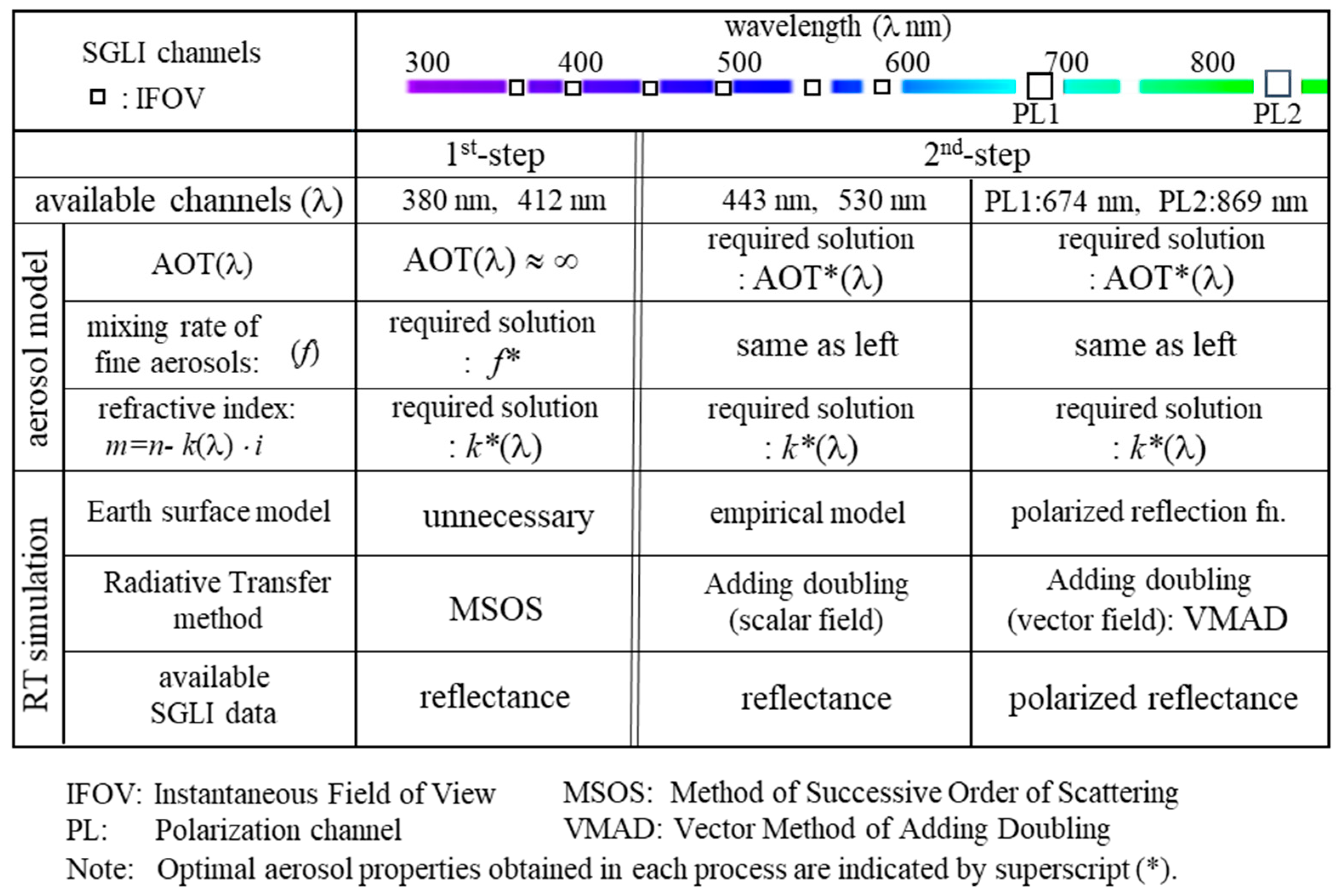
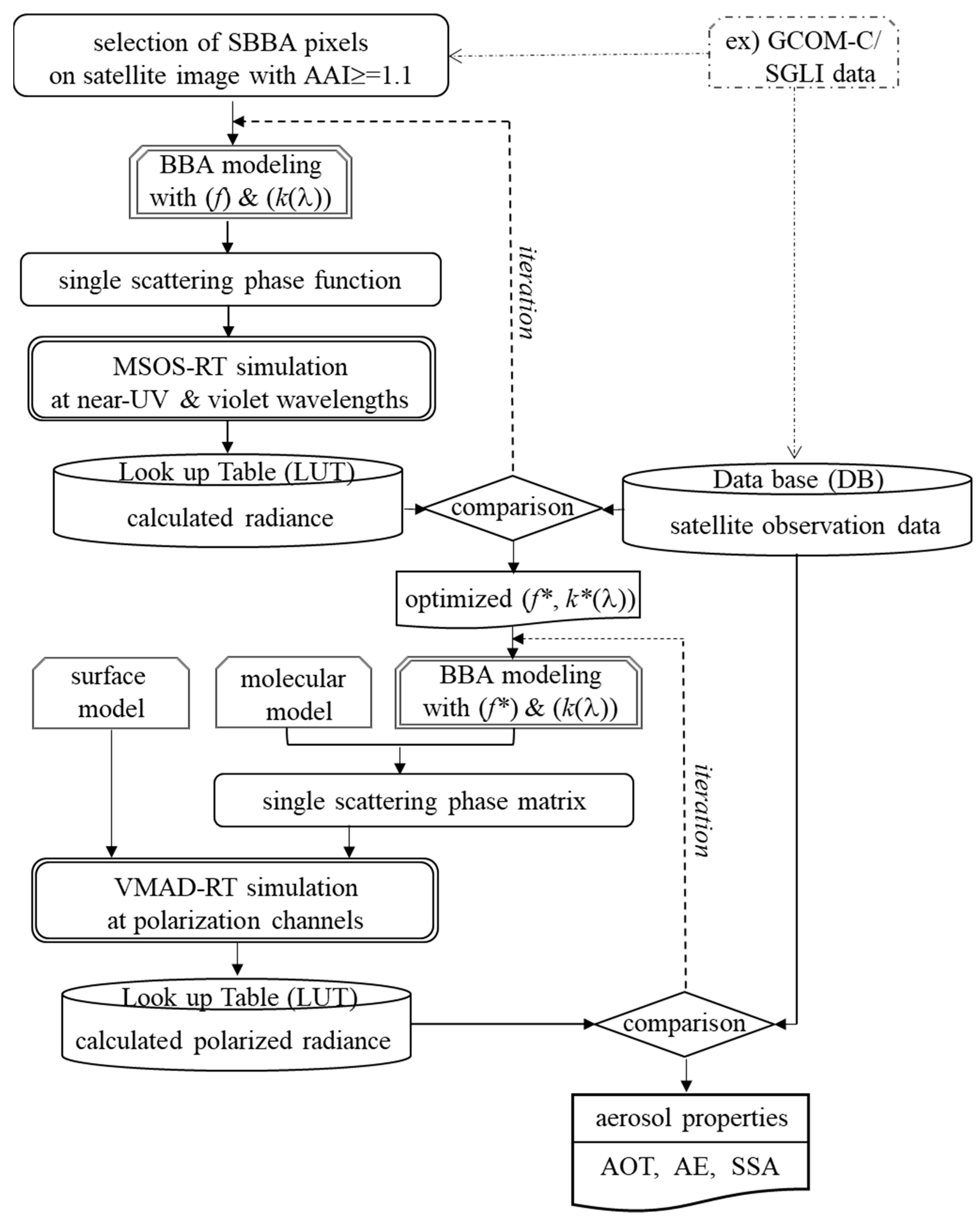
2.1. Construction of an Aerosol Retrieval Algorithm Using Satellite Observations

The aerosol retrieval process comprises two parts: aerosol modeling and radiation simulation, in a combined system of Earth’s atmosphere and surface. Key components of the Earth’s atmosphere–surface system are atmospheric aerosols, various atmospheric gases, and the Earth’s surface; these components have been well-described by low-resolution atmospheric transmission 7 (LOWTRAN 7) and the International Geosphere-Biosphere Program (IGBP). Our previous work described the basic flow of an aerosol retrieval algorithm for severe wildfires using satellite observations [23]. This current study builds on those calculations.
Aerosol modeling is the beginning of the algorithm workflow and is fundamental to the efficiency of subsequent processing. In our previous work, the AAI (absorbing aerosol index) proved to be an effective method for the detection of absorbing aerosols, such as carbonaceous aerosols or mineral dust [22]. The AAI calculation is as follows:
AAI = R (412)/R (380)
where R represents the observed SGLI reflectance at wavelengths of near-ultraviolet (UV; 380 nm) and violet (412 nm).
Our AAI index follows the Total Ozone Mapping Spectrometer-Aerosol Index (TOMS-AI) concept [28]. Once the aerosol type has been approximately predicted, it is useful for the efficiency of the subsequent retrieval of the aerosol properties. The determination of BBA types using the AAI index is based on the statistical analysis of SGLI data from 2018–2019. When AAI ≥ 0.83, the presence of BBAs is indicated [22]. When AAI > 0.95, high levels of BBAs are being produced from severe biomass burning areas [23]. After we included SGLI data from 2020 and later, we found that the most intense wildfires measured AAI ≥ 1.1, which is useful for the detection of extreme SBBAs. It is interesting to note that although the AAI value for BBA increases with optical thickness for wildfires, the same results are not found with the AAI values of desert dust and clouds. Desert dust and clouds initially show a similar optical thickness, but the AAI values converge around 1.0. These results are only derived from the processed SGLI data at present and require further examination based on simulation calculations.
The basic aerosol property to define is the spectral aerosol optical thickness (AOT) (λ) at the wavelength (λ nm) [24]. Then, we quantify the aerosol size distribution, which is represented by bimodal (fine and coarse) log-normal distributions of the particle volume (according to the automatic classification of accumulated NASA/AERONET data) [29]. We have shown that aerosol size distribution can be expressed by a simple approximation with the unique variable of the fine particle fraction (f) of the volume concentration (Appendix A).
The third item that comprises the aerosol properties is the complex refractive index, given by the calculation (m = nk·i). The real part (n) and imaginary part (k) of the complex refractive index are given as parameters. In our system, n is freely selectable in the range from 1.35 to 1.6, and k is freely selectable in the range from 0.0003 to 0.1. In the current study, we assume n = 1.5 or 1.55 for BBAs, and k is the only variable parameter. Using this method, we can account for spectral absorption (especially in the near-UV wavelengths) [30,31].
The next step in the aerosol retrieval process is to calculate the radiative transfer (RT) in the combined atmosphere–underlying surface system using vector RT codes [32]. The information on the Stokes vector of reflected light is particularly useful for aerosol retrieval, especially in moderate AOT atmospheres, because the degree of polarization tends to decrease due to the higher order of multiple light-scattering events. This is because aerosol particles polarize the incoming natural light, and the emerging light polarization is depressed by multiple scattering effects, which leads to an increase in entropy of the reflected light field.
Our aerosol retrieval algorithm consists of two steps for processing GCOM-C/SGLI data (Figure 1). First, we consider the scalar RT equation for a thick atmosphere by introducing a radiation simulation method called the method of successive order of scattering (MSOS). The MSOS applies the classical successive scattering method, i.e., calculating the reflectance from an optically semi-infinite atmosphere model. In the current study, the MSOS is used to calculate the upward intensity of radiation at the top of the atmosphere at τ   [23]. The contribution of reflection from the bottom Earth’s surface is not considered because we include an optically thick absorbing light-scattering layer. Severe wildfire events produce large amounts of BBAs, and especially high values of AOT are expected in the shorter wavelength regions of λ = 380 nm and 412 nm (Figure 1, 1st step). In this first step, we obtain the parameter (f) for the aerosol size distribution and the imaginary part of the refractive index (k). In the second step, both (f) and (k) are good candidates for the initial approximation of longer wavelengths.
Next, we adopt a vector-type RT simulation method to utilize the SGLI polarization band level (PL1 and PL2) (Figure 1). We apply an RT simulation for the atmosphere–surface system using the vector method of adding–doubling (VMAD) [32]. Bottom surface reflection cannot be avoided in RT simulations in a finite AOT atmosphere. Therefore, the polarized reflectance of the bottom surface is described by the Bi-directional Polarization Distribution Function (BPDF), as given by the Polarization and Directionality of the Earth’s Reflectance (POLDER) [33]. The bottom surface reflection has a small influence on the results in an opaque atmosphere [32]. Polarization information is a key indicator of aerosol properties, signaling that the two polarization channels of SGLI (PL1: 674 nm; PL2: 869 nm) can be used for aerosol retrieval. The ability to use SGLI data and to switch between scalar and vector RT simulations is an advantage of our method, and this process is not limited to polarization channels only (Figure 1, 2nd step). Radiance is used for visible channels at 443 nm and 550 nm. Finally, values for AOT, Ångström Exponent (AE), and single scattering albedo (SSA) are obtained. AE values are derived from AOT (869 nm) and AOT (443 nm). SSA values are calculated for each pixel of satellite data as the ratio of the scattering and extinction coefficients of the aerosol model (Figure 1).
The flow of the retrieval algorithms for SBBAs using satellite data is given in Appendix B; Figure A1 illustrates the block flow of SBBA retrieval from satellite data.

2.2. Regional Model Simulation of Wind Movement over Complex Terrain

The SCALE regional model was used to investigate the effect of terrain on airflow. The accuracy of SCALE winds has been found to be acceptably accurate [34]. We ran a SCALE simulation at a resolution of 5 × 5 km grids, and we based surface heights on the United States Geological Survey model GTOPO30 (a global digital elevation model with a horizontal grid spacing of 30 arc seconds).
A single run by SCALE started at 00:00 Coordinated Universal Time (UTC) on a date in the period and stopped after 30 h. We discarded 6 h from the initial time as the spin-up. The initial conditions and boundary conditions included east–west and north–south winds, temperature, relative humidity, and atmospheric pressure from the National Centers for Environmental Prediction (NCEP) operational global analysis data. NCEP products were provided by the Global Data Assimilation System, which continuously collates observational data from the Global Telecommunications System and other sources.
To investigate the effects of topography, the meteorological simulation was first run using a flat region, then run with actual terrain, and the results of both simulations were evaluated. By comparing the two simulations, the impact of topography on wind field could be revealed.

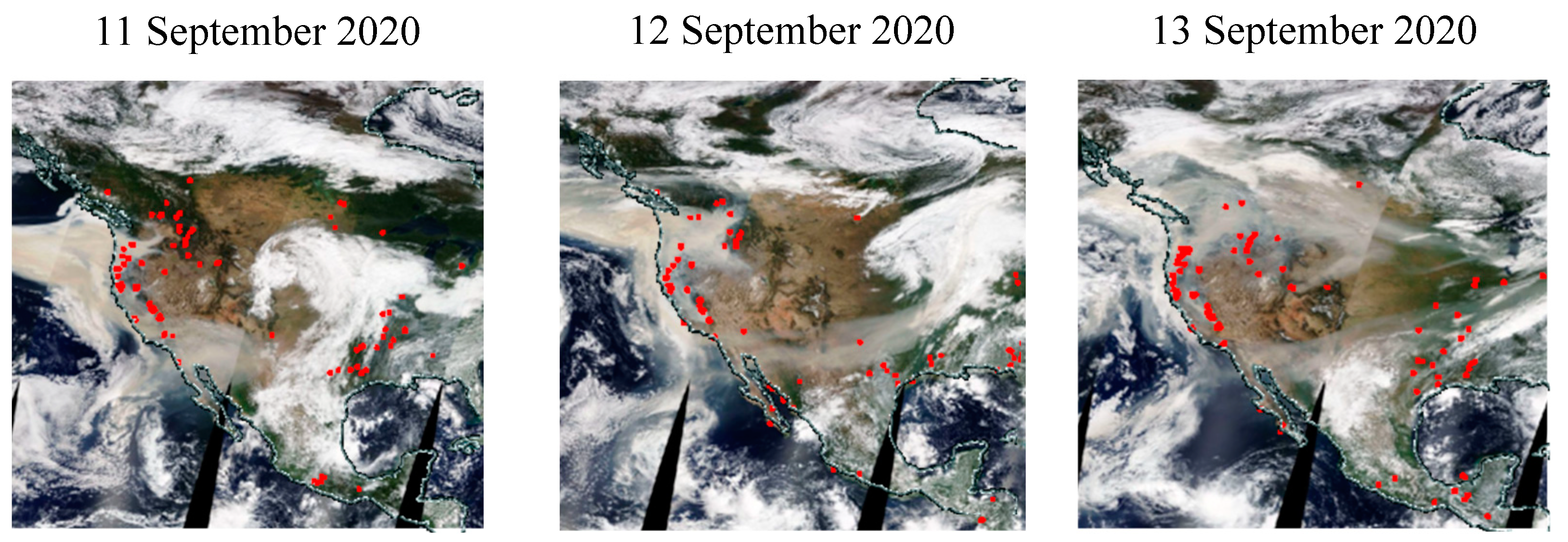
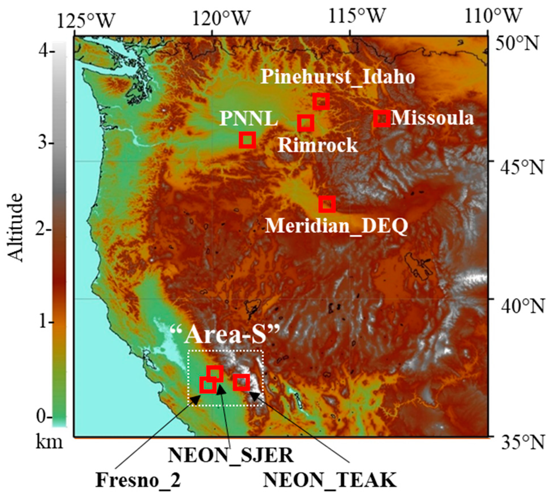
2.3. Search Strategy for the Target Study Area

Satellite images provide a bird’s eye view of the movement behavior of wildfire-generated aerosols. The hotspot information from satellite thermal data can identify the location and intensity of the source(s) of a wildfire. Figure 2 shows the NASA/World View (WV) in the United States, using Terra/MODIS/MOD14 from 11 to 13 September 2020 [35]. The images are true color composites, and the hot spots are represented by red dots. The images depict large wildfires that occurred in the forested areas along the Pacific coast, and the gradual attenuation of the wildfires as they spread into the interior of the United States. In more recent years, the wildfires of western North America have become more severe, with the size and intensity of wildfires increasing over time [36,37]. The risk and damage caused by wildfires have become inevitable, not only in the United States, but also in the Amazon and South Africa [37,38,39]. We used data from the western North American severe wildfires of September 2020 to characterize the atmospheric aerosols.
We charted meteorological data (such as wind speed, temperature, and relative humidity) over the same time from the NCEP Final Model (NCEP-FNL) (Figure 3). We compared these data with the data collated from TERRA/MODS/MOD14 and confirmed that the data were consistent across both data providers [40]. We plotted the wind speed at 850 hPa to visually comprehend the atmospheric movement (Figure 3a). The air mass flow in Figure 2 and described above agreed with the wind-behavior data of the upper atmosphere. The Pacific Northwest of the United States was extremely dry and hot during this period. It is not clear whether these meteorological conditions triggered wildfires or whether the wildfires caused the hot and dry climate. In any case, both factors contributed to a wildfire perpetuating cycle.
The subsequent sections of our methodology focus on the dry and hot areas that correspond to latitude [N35,N50] and longitude [W110,W125] and are indicated by the black squares in Figure 3b,c. A topographic map of the selected study area is illustrated in Figure 4. The positions of the target AERONET sites are marked by red squares [41], and Area-S is the plotted area that is enclosed by a white dotted line. There are three AERONET sites within Area-S: Fresno_2, NEON_SJER, and NEON_TEAK. We selected Area-S as it meets the requirements of this study, i.e., hazy aerosols caused by severe wildfires across complex terrain and access to high-quality ground-based datasets. The ground-based NASA/AERONET measurements of AOT in Area-S constitute a particularly useful dataset for the validation of our retrieval algorithms. The ground-based measurements are also essential to validate the aerosol characterizations that we developed from satellite data.
The GCOM-C satellite is a high-resolution polar-orbiting satellite with a narrow swath. This orbital track means the SGLI does not often encounter intense wildfires; however, the satellite did observe the wildfires within Area-S on 12–13 September 2020, producing the images given in Figure 5. The key data retrieval AERONET stations within Area-S are shown as open red squares on the SGLI images at 19:13 (UTC) on 12 September (Figure 5a) and at 18:47 (UTC) on 13 September (Figure 5b). The marked AERONET stations are Fresno_2 (36.8°N, 119.8°W), NEON_SJER (37.1°N, 119.7°W), and NEON_TEAK (37.0°N, 119.0°W) of NASA/AERONET.
Hot-spot data provided by Terra/MODIS/MOD14 were plotted as three levels of wildfire radiative power: red dots ≥ 200 MW; orange dots 100–200 MW; dark-yellow dots 100 MW [36]. The SGLI has observation channels in the near-UV wavelength range, and the channels for the three primary colors shifted to shorter wavelengths than usual to accentuate the smoke (Figure 5). The R, G, and B bands were observed at 443 nm, 412 nm, and 380 nm, respectively.
As the atmosphere became optically thicker due to wildfire smoke, it became difficult for the satellite to observe vegetation and the ground surface. The brown color spreading in the center of the figure denotes the dense smoke caused by SBBAs. The beige color beneath the thick smoke suggests the presence of an optically thick haze. Heavy wildfires were observed to be burning around (37.5°N, 119.3°W) and (36.2°N, 118.6°W), and on both days, thick smoke was seen coming from these wildfire sources in the vicinity of the three AERONET sites. These conditions suit our experimental requirements to select SBBAs as the target of analysis to elucidate optically thick hazy aerosols. Thick aerosols such as these are usually left as ‘undetermined’ in the satellite data as NASA/MODIS products MOD04 and MYD04, and JAXA/SGLI/L2 products. A thick rod-shaped air mass appeared in the image shown in Figure 5b, which demonstrates the very thick smoke rising in the air. This interesting target is further discussed later in the paper.

3. Results

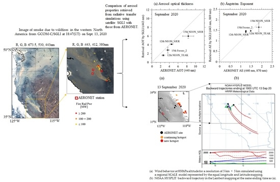
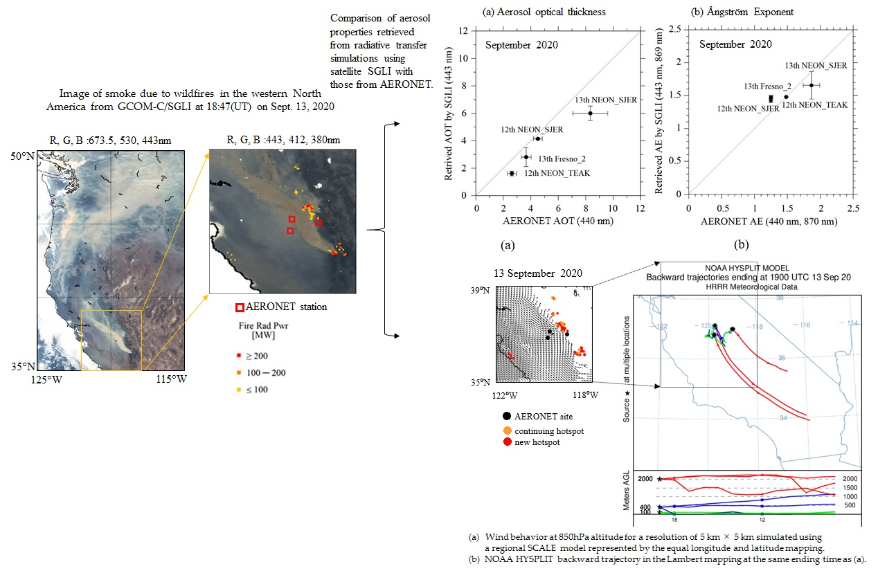
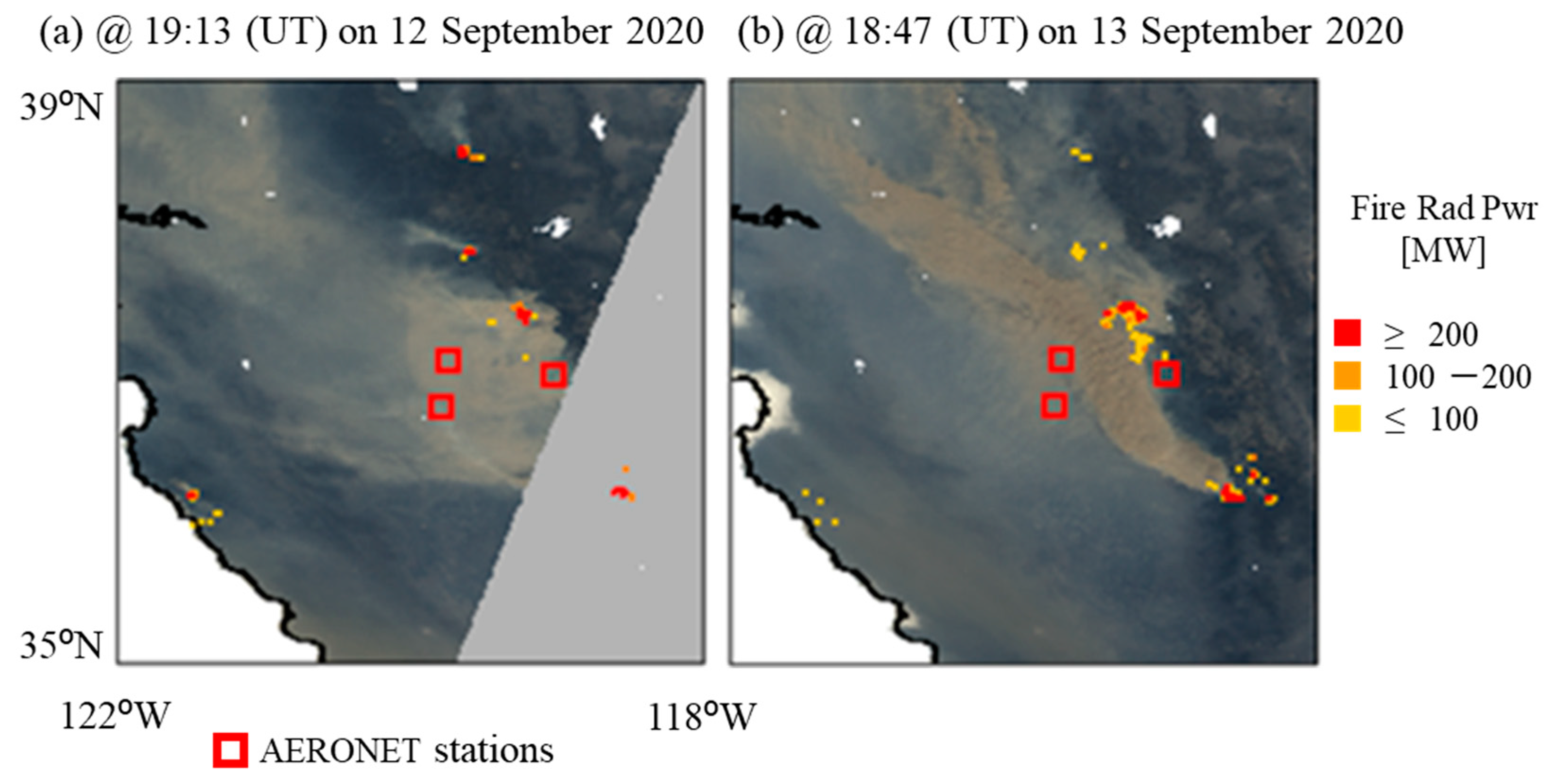
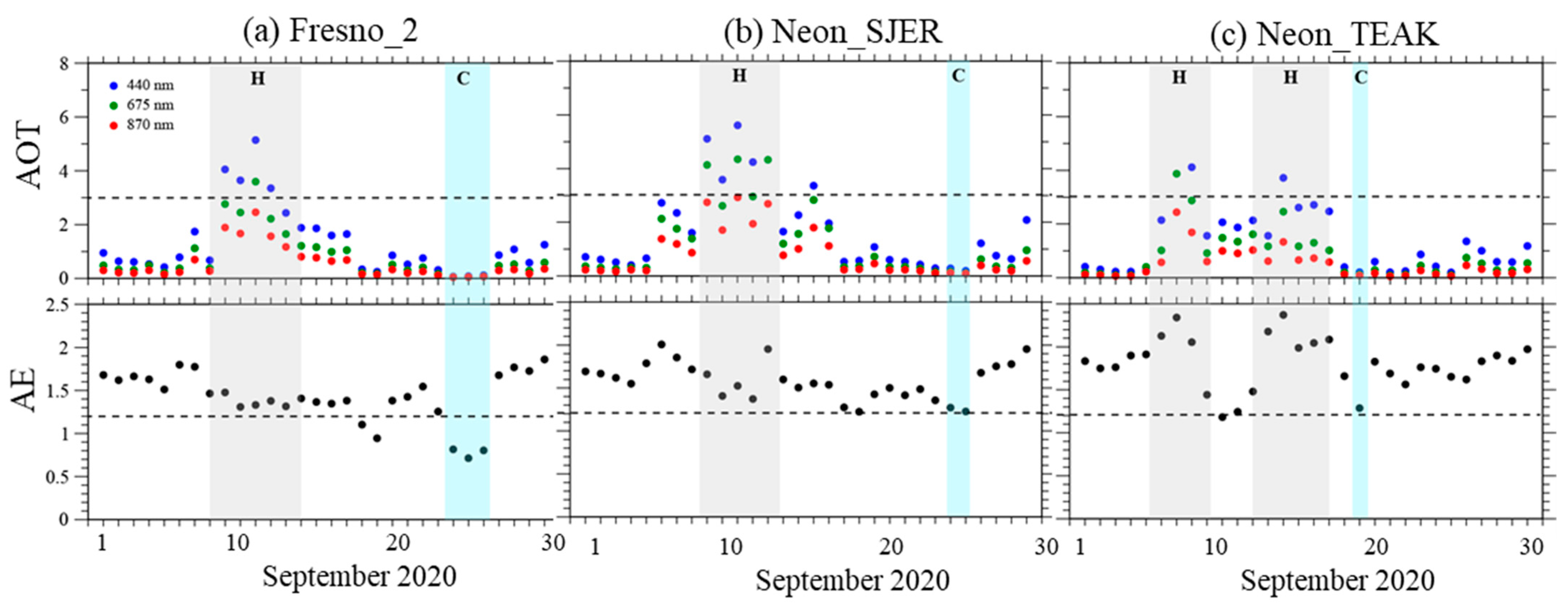
3.1. Ground-Based Remote Sensing of Aerosols

The daily average of AOT (λ) and AE for Area-S are displayed in Figure 6. AOT decreases with wavelength. The highest average values of AOT (≥3) are represented by the dashed line and correspond to hazy atmospheres. The smallest average values of AE (≥1.2) are represented by the dashed lines and correspond to small aerosol particles.
A hazy atmosphere (consisting of small particles such as BBAs) is indicated when both the AOT and AE average values are high (charted as the gray vertical bands (H)). All three AERONET sites indicated a hazy atmosphere on 12–13 September 2020. A clear atmosphere (consisting of small aerosol particles) is indicated when both the AOT and AE average values are low (charted as the blue vertical bands (C)). One can imagine a clear California sky with small oceanic aerosols corresponding with the Fresno_2 site measurements of very low AOT and AE values (Figure 6a). In contrast, both the NEON_SJER and NEON_TEAK sites measured higher average AE values despite a clear atmosphere (Figure 6b,c). This may be explained sufficiently by clear days containing smaller particles on average at both the NEON_TEAK and NEON_SJER sites when compared with the hazy days.
The altitudes of the three AERONET sites are different: Fresno_2 (100 m), NEON_SJER (368 m), and NEON_TEAK (2147 m). The daily average values of AE at NEON_TEAK were predominantly high throughout September. This suggests that the altitude of each site needs to be considered in relation to the results, even when sites are located relatively close to each other. We know that these sites have a complex topography that influences the way that wind moves (Figure 3 and Figure 4). In order to understand how complex topography influences aerosol dynamics and optical properties, it is necessary to combine the data from regional numerical models with ground-based data and satellite observations.
Although we observed a variation in wavelength measurements, the values of the SSA were unexpectedly high (>0.85) at all three sites in September 2020.
We calculated the AAI distribution from SGLI/Level-1B data for 12–13 September 2020 and charted the results for Area-S (Figure 7). The three AERONET sites are denoted by the red squares in the lower-left area of the chart. The image demonstrates that Area-S is within an area where AAI > 1.1, exceeding the threshold value for detecting SBBAs, confirming that the three AERONET sites are suitable targets for SBBA analysis.
We observed an interesting phenomenon within Area-S. A thick-stream type of shape is evident with an elevated AAI > 1.1 (Figure 7b). This shape generally matches the shape of wildfire smoke seen by satellite observation data (Figure 5b). Both shapes occurred on 13 September 2020.

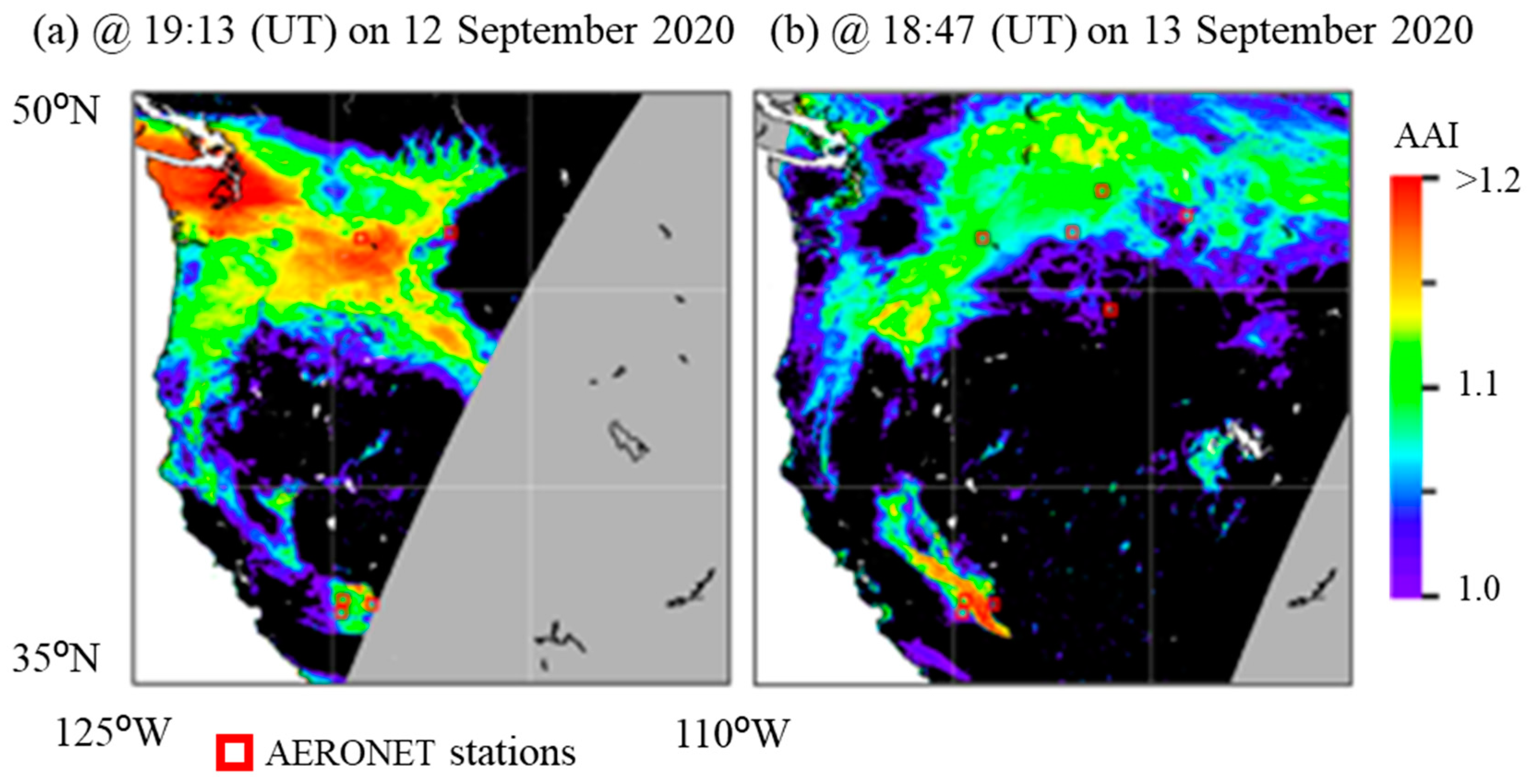
3.2. Comparison with Satellite-Based Characterization of Aerosols

Previously published work has demonstrated that an area with high AAI values correspondingly has high AOT values [22], and our results for Area-S confirm this finding (Figure 6 and Figure 7). One of the issues is that most of the current official aerosol products (such as MODIS products MOD04 and MYD04, and SGLI/L2 products) do not retrieve aerosol properties over areas with a high AOT value.
We used a two-step process to retrieve aerosol properties from SGLI measurements (see Section 2.1). The first part of the process extracted the ratio of the fine-mode and coarse-mode fractions of the bi-modal size distribution. Complex refractive indices were assumed based on the semi-infinite atmosphere model. Because the model assumes that surface reflectance does not contribute to signals at the top of the atmosphere, this model can only be applied over high AOT areas, that is, high AAI areas.
We expected regions that measured AAI ≥ 1.1 to have an AOT > 3 [22]. Once we obtained the mode fractions of the fine and coarse model aerosols and complex refractive indices, and based on an ordinary (finite) vector RT model, to include the polarization information of 674 and 869 nm, we used this information in the second part to retrieve AOTs at wavelength λ.
The retrieved results of aerosol properties were partially validated by ground-based observations using AERONET. In this study, AERONET stations Fresno_2, NEON_SJER, and NEON_TEAK, which are close to the wildfire plume, were selected. However, some of the AOT (440 nm) measurements on the 13th at NEON_SJER are not available due to the very dense plume conditions [42]. Therefore, we decided to estimate the value of AOT (440 nm) from AERONET’s measurements of AOT (670 nm) and Ångström exponent (AE) using Equation (2):
A O T   ( 440   nm ) = A O T   ( 670   nm ) ( 440 670 ) A E
We compared the aerosol properties calculated from ground-based observations with those calculated from satellite observations (Figure 8). We used the average of the AERONET measurements taken within ±30 min of the GCOM-C/SGLI overpassing Area-S. We similarly retrieved results for aerosol properties from SGLI when the SGLI was within ±0.05° (latitude–longitude coordinates) of the Area-S AERONET sites. The acquired AOT and AE are shown in Figure 8a and Figure 8b, respectively. The obtained aerosol properties as AOT and AE from both data collection methods agree closely with each other.
The retrieved SSA from SGLI at this site gave 0.82 ± 0.02 (standard deviation) at 443 nm. Our retrieved results indicate the existing more absorbing particles in the atmosphere. We can assume that the difference between the retrieved results and the AERONET measurements comes from the difference in the optical properties of particles at the top and bottom of the plume layer in dense-aerosol conditions.
For comparison of the SSA, we selected only the measurement from the Fresno_2 site at 18:58 on 12 September 2020. The Fresno_2 hybrid measurement of SSA was 0.92 at 440 nm. The Fresno_2 SGLI data measurement of SSA was 0.89 ± 0.01 (standard deviation) at 443 nm. These results show that the SGLI measurements are in close agreement with the ground-based measurements. Other SSA measurements from AERONET may not be available, even with the hybrid method, because of the lack of symmetric atmospheric conditions in the almucantar or because the aerosol layer is too complex.
Not every AERONET site shown in Figure 4 was available for the measurements. Therefore, the number of validation points was limited. The stochastic analysis was not reasonable though; the correlation coefficients between our simulated results and the AERONET measurements were approximately 0.9 for both AOT and AE.

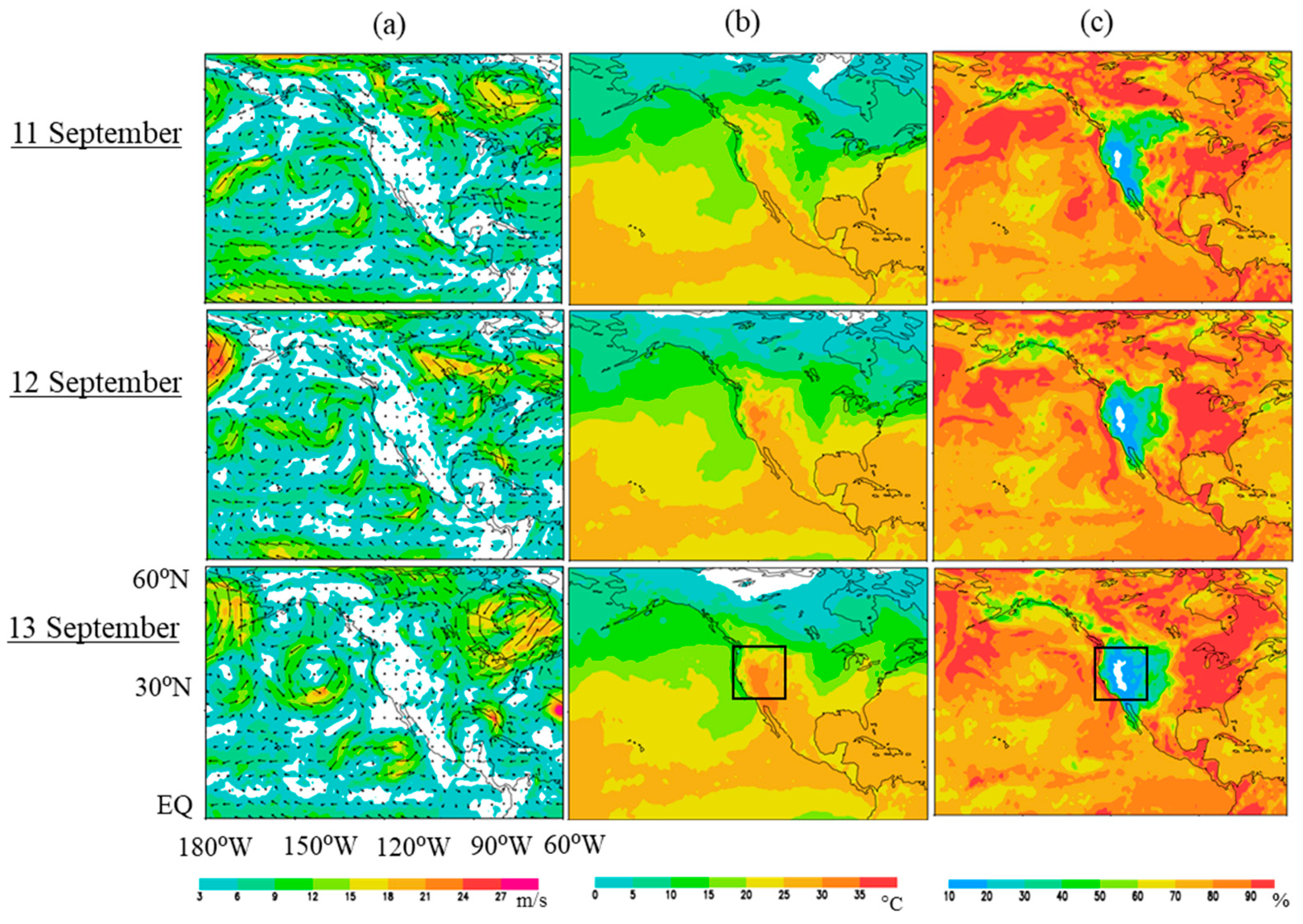
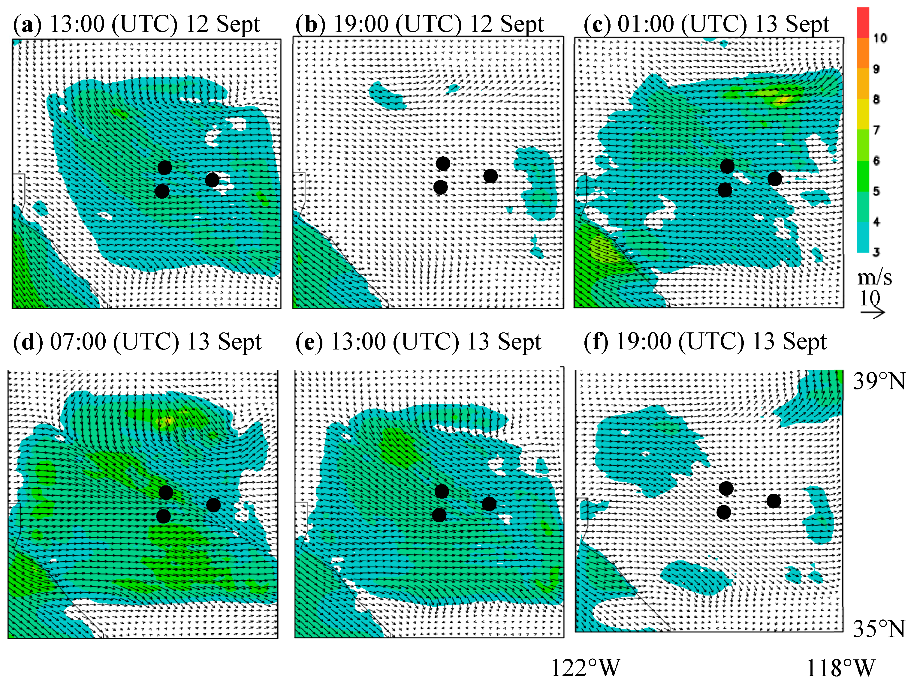
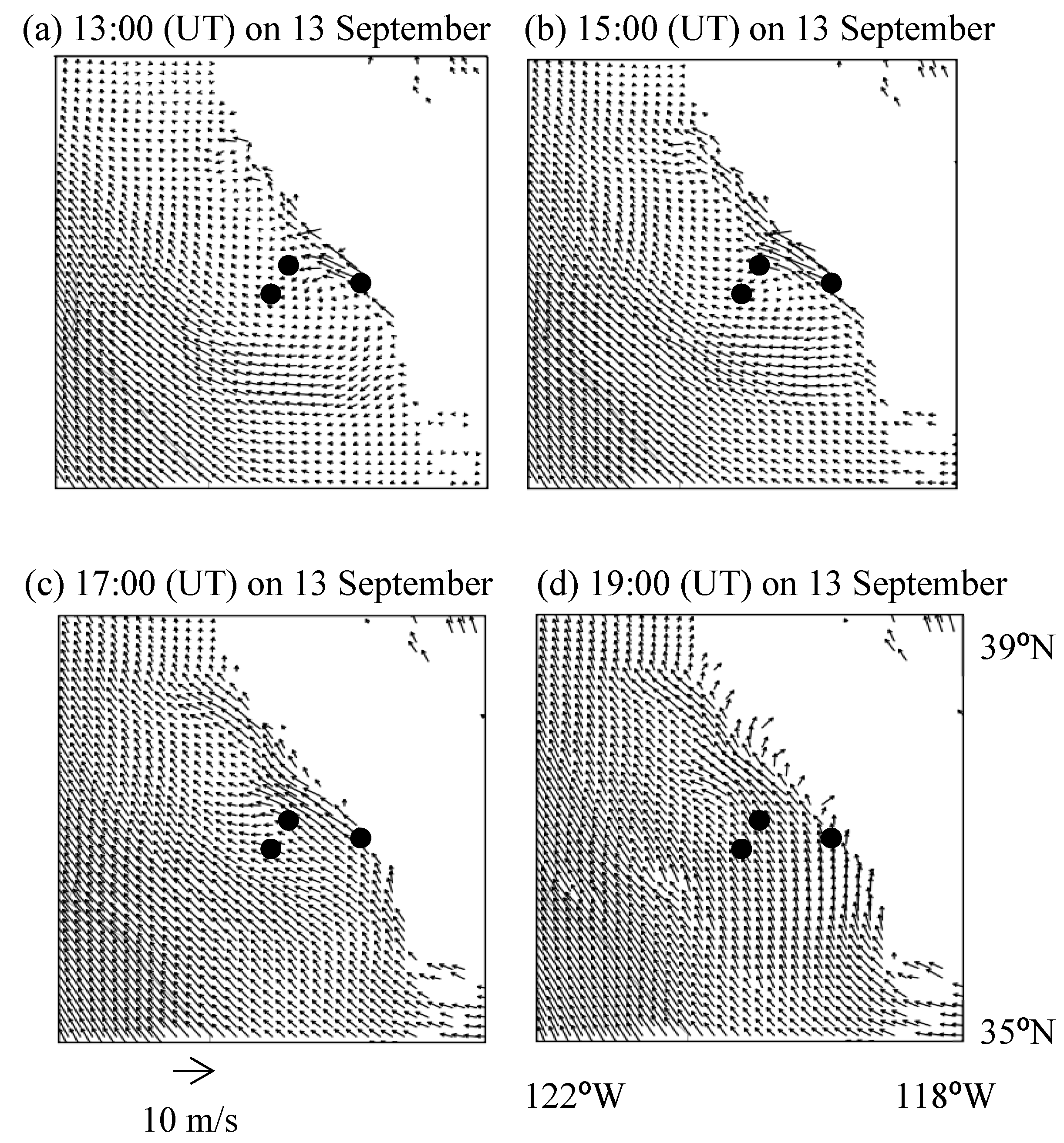
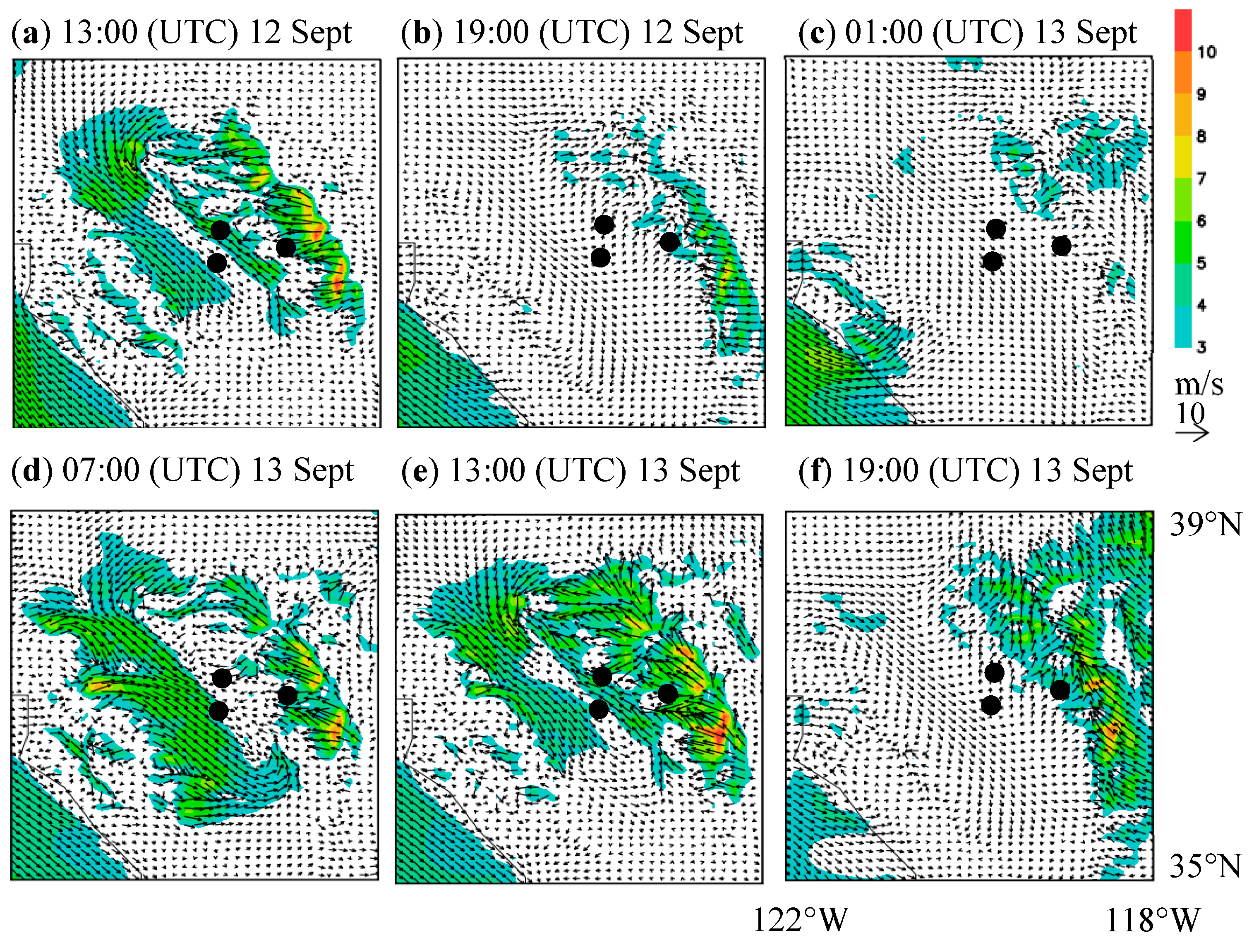
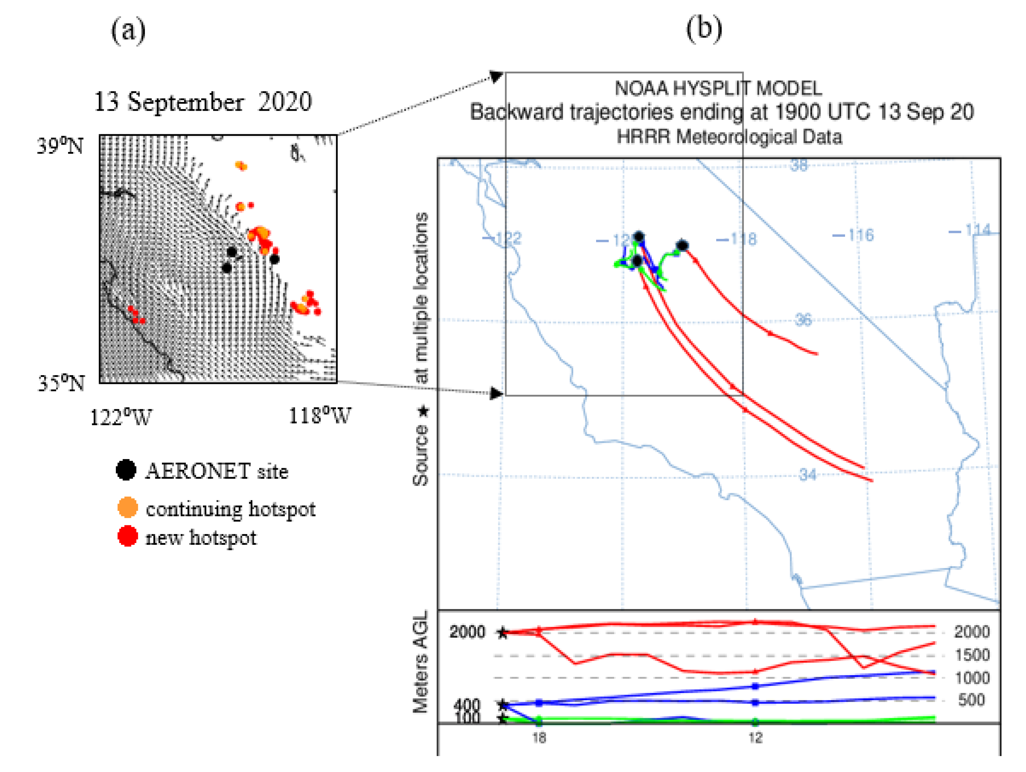
3.3. Regional Meteorological Modelling of the Wind Transfer of Aerosols

We compared observations from space with winds simulated by a regional meteorological model to investigate the dynamics of airflow and dispersion of atmospheric particles. We plotted the results of the SCALE simulation for near-ground wind behavior in Area-S, with a resolution of 5 km × 5 km (Figure 9). To provide detail on the wind characteristics, we produced images for each 6-hour period between 13:00 (UTC) on 12 September and 19:00 (UTC) on 13 September 2020 (Figure 9a–f). In terms of the observation period, Figure 9b and Figure 9f corresponds to Figure 5a and Figure 5b, respectively.
During the observation period, the winds at Fresno_2 always blew from the northwest, flowing inland from the Pacific Ocean, and wind speeds were lower during the day. At NEON_TEAK, the prevailing wind originated from the east, which was very different from Fresno_2. We suggest that this difference resulted from complex wind movements that were blocked and that bounced back from the high mountains that rise to the east side of the NEON_TEAK site. The winds at NEON_SJER were more changeable, blowing from the southeast in the early morning (opposite to the winds of Fresno_2), then changing to the northwest in the evening.
Comparing the satellite image of smoke and hot spots in Figure 5a with the wind simulation results in Figure 9b, we can see that smoke drifted around the Area-S sites at approximately 19:00 (UTC) on 12 September 2020, and weak winds spirally converged. This indicates that the smoke generated near hot spots drifted and caused an increase in the AOT measurements at these sites, as shown in Figure 6. The satellite image of the next day (13 September) shows thick smoke flowing in a northwesterly direction near the southeastern hot spots (Figure 5b). Our wind simulation results indicate that when the wind blew from the northwest, dark smoke flowed along the boundary between the plains. When the wind blew from the east, dark smoke flowed along the mountainous area. Thick smoke appeared to flow along the mountain range.
In any case, a high AOT was observed at the three AERONET sites during this period, owing to the smoke from wildfires (Figure 6). The fact that Fresno_2 was affected by the smoke for a shorter period than the other two sites on 12–13 September 2020 may be related to the fact that Fresno_2 is more distant from the wildfire source than the other sites; therefore, it was less affected by the smoke due to the predominant wind direction.
We then ran a comparative near-ground wind simulation with the same conditions and period, but with topographical effects removed (no ground undulations) (Figure 10). The tendency for wind speed to weaken during the day occurred when complex terrain was included. When the terrain was complex, the wind direction was different at each AERONET site (Figure 9), but in the simulation without topography, the wind direction was the same at all sites (Figure 10). This means that the wind direction, which changes in a complex manner depending on the time of day, and the site are greatly influenced by topography.
The shape and thickness of the smoke plume on 13 September 2020 had several peculiarities. To analyze the flow of this plume, we ran a comparative SCALE wind simulation at an altitude of 850 hPa at 2-h intervals from 13:00 to 19:00 (UTC) on 13 September 2020 (Figure 11). The simulation results indicate that an almost-uniform southeast wind blew during this period. The results suggest that the surface-generated wildfire was fueled by the winds on the ground. As the influences of complex topography came into effect, the wildfire rose onto the strong southeast winds that blew from above, which formed a long smoke mass extending from the southeast to the northwest (as seen in Figure 5b). The complex twisting pattern can be interpreted as convection due to the optically thick haze and the difference in wind direction between the bottom and top layers. The smoke mass from the southeastern fire source drifted with the southeasterly wind and combined with the smoke mass from another fire source, which resulted in the interesting smoke shape captured by the satellite image in Figure 5b.

4. Discussion

The aerosol properties that we retrieved from the SGLI satellite observation data were confirmed by the aerosol properties retrieved from the AERONET ground-based observation data. We found that both methods provided wind behavior data that were similar to those produced by the regional SCALE model. SCALE simulations showed that the smoke flow generated by wildfires can be described in terms of the wind field.
The behavior of wind at an altitude of 850 hPa was simulated by SCALE for the SGLI passing time and the hot spots, and the orange and red dots represent both continuing wildfires and new wildfires, respectively (Figure 12a). The Hybrid Single-Particle Lagrangian Integrated Trajectory (HYSPLIT) model proposed by the National Oceanic and Atmospheric Administration (NOAA) was adopted to analyze the airflow back trajectory of pollutants on 13 September 2020, as shown in Figure 12b. Airflows at heights of 100 m, 400 m, and 2000 m were selected to correspond to the altitudes of the three AERONET sites shown in Figure 12a, and back trajectory diagrams were calculated. In Fresno_2, the near-surface air masses were transported from a northwesterly direction, while in NEON_SJER, they were transported from a southeasterly direction, consistently with the behavior of the near-surface wind simulated by SCALE shown in Figure 9. The airflow influenced the air masses at 2000 m from the southeastern direction at three AERONET sites.
It can be seen from these results that the wildfires spread, and the impressive thick bar-shaped air masses shown in Figure 5b were formed by very heavy smoke rising from the hot-spot clusters found around (36.2°N, 118.6°W) and (37.5°N, 119.3°W), carried by the southerly wind. By combining simulated winds and back-trajectory analyses, we can obtain a more detailed picture of how the smoke distribution in satellite imagery is caused by airflow influenced by topographic effects.
We suggest that complex mountain topography drives airflow through wind dynamics at the regional scale, which influences changes in atmospheric particle properties, even within a small region. In the future, it is necessary to investigate the movement of atmospheric particles in more detail by conducting simulations using a regional chemical transport model. As a first step toward the quantitative assessment of atmospheric particles, it is essential to improve the practicality of regional models based on an accurate estimation of emissions [43,44].
Further use of polarization information should be considered in future research. SGLI is a follow-on sensor for the POLDER series on ADEOS-1, -2, and the Polarization and Anisotropy of Reflectances for Atmospheric Sciences coupled with Observations from a Lidar (PARASOL) and has unique capabilities for polarization measurements [45,46]. The sensor was designed to acquire Stokes vector components (I, Q, and U) at two wavelengths, 674 nm and 869 nm, with a 45° forward/backward tilt capability to measure scattered light at moderate scattering angles (from ~90° to ~120°). The development and operation of an SGLI-like future instrument equipped with multidirectional observation and polarized multi-channels (particularly in UV and SWIR) are desired. EUMETSAT/EPS-SG/3MI, which is expected to be operational by 2024, is awaited. In addition, polarization observation has been proposed as an interesting Earth-observation satellite project [47].

5. Conclusions

In this study, we characterize the BBAs from wildfires that occur frequently in the Pacific Northwest of the United States, a complex topography of basins among mountains along the coast. We provide the following conclusions from our results:
  • BBAs can be effectively detected using MODIS/hotspot, AERONET data, the regional model SCALE with NCEP-FNL, and our aerosol type classification index AAI (derived from near-UV measurements by GCOM-C/SGLI);
  • We improved our retrieval algorithm for SBBAs to achieve more accurate solutions, especially regarding AOT;
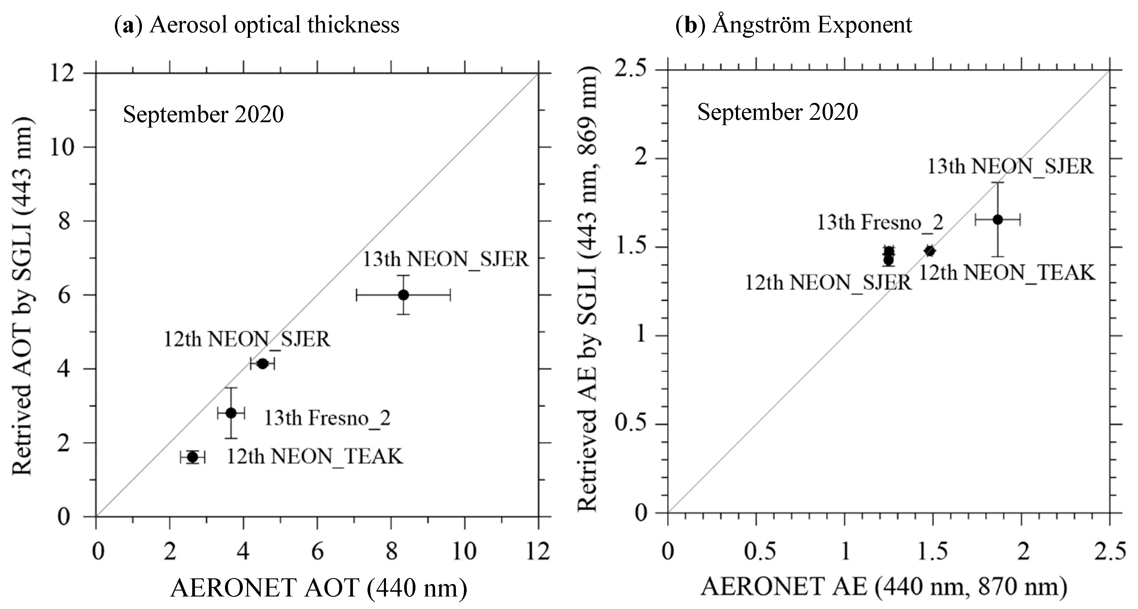
  • The aerosol properties that were obtained by our retrieval method using SGLI data were consistent with the ground-based observations of AERONET;
  • Finally, our retrieved results were validated with wind behavior by the regional model SCALE.

Author Contributions

Conceptualization, M.N. and S.M.; system analysis and creation, I.S.; investigation, M.N., S.M. and A.K.; writing—original draft preparation, M.N., I.S. and S.M.; writing—review and editing, all authors; project administration, S.M.; funding acquisition, S.M. and I.S. All authors have read and agreed to the published version of the manuscript.

Funding

This research project was funded by the Global Change Observation Mission-Climate (GCOM-C) project by the Japanese Aerospace Exploration Agency (JAXA) (No. JX-PSPC-530188), JSPS KAKENHI Grant Number 19h04242, and the Beyond Europe Project (GRASP-cloud) by the Austrian Research Promotion Agency (FFG).

Acknowledgments

The authors would like to thank Toshiyuki Fujito for assisting in preparing the satellite data, and NASA and JAXA for distributing the observed data with Terra/MODIS and GCOM-C/SGLI, respectively. The authors would also like to thank the PIs of the AERONET stations that allowed us to use data in this work and NASA/AERONET.

Conflicts of Interest

The authors declare no conflict of interest.

Appendix A

Approximation of aerosol size distribution
The size distributions are assumed to be two modes (fine and coarse) in a bimodal log-normal distribution of the particle volume with six parameters [30]. The calculation is as follows:
d V d ln r = V f 2 π ln σ f exp [ ( ln r ln   r f ) 2 2 ln 2 σ f ] + V c 2 π ln σ c exp [ ( ln r ln   r c ) 2 2 ln 2 σ c ] .
where
  • V is the particle volume;
  • subscript f are fine mode particles;
  • subscript c are coarse mode particles;
  • Vf, Vc are volume concentrations;
  • rf, rc are mode radii;
  • σf, rc are standard deviations.
Six parameters are too many for the retrieval of optimized aerosol sizes from satellite observations. Therefore, we simplified the aerosol size distribution function by using the average value of mode radius and the maximum value of the standard deviation among the continental aerosol models (accumulated data from NASA/AERONET). The parameter values for the approximate size distribution are given in Table A1 [22].
Using the size distribution function enables continental aerosols to be approximated by the unique variable of the fine mode particle fraction (f). This fraction is derived from the volume concentration calculation as follows:
f = Vf/(Vf + Vc).
Table A1. Parameters of approximate form of Equation (A1).
rf (μm)σf (μm)rc (μm)σc (μm)
0.1441.5333.6072.104

Appendix B

Process flow used for the development of severe biomass burning aerosol (SBBA) retrieval algorithms from satellite observations.
Figure A1. Block flow diagram of the process used to develop severe biomass burning aerosol (SBBA) retrieval algorithms from satellite observation data at wavelength λ. Optimal aerosol properties obtained in each process are indicated by superscript (*).
Remotesensing 14 02344 g0a1

References

  1. IPCC. Climate Change 2021: The Physical Science Basis; Contribution of Working Group I to the Sixth Assessment Report of the Intergovernmental Panel on Climate Change; Cambridge University Press: Cambridge, UK, 2021. [Google Scholar]
  2. IPCC. Climate Change and Land: An IPCC Special Report on Climate Change, Desertification, Land Degradation, Sustainable Land Management, Food Security, and Greenhouse Gas Fluxes in Terrestrial Ecosystems; IPCC: Geneva, Switzerland, 2019. [Google Scholar]
  3. Landis, M.S.; Edgerton, E.S.; White, E.M.; Wentworth, G.R.; Sullivan, A.P.; Dillner, A.M. The impact of the 2016 Fort McMurray Horse River Wildfire on ambient air pollution levels in the Athabasca Oil Sands Region, Alberta, Canada. Sci. Total Environ. 2018, 618, 1665–1676. [Google Scholar] [CrossRef] [PubMed]
  4. Liu, J.C.; Pereira, G.; Uhl, S.A.; Bravo, M.A.; Bell, M.L. A systematic review of the physical health impacts from non-occupational exposure to wildfire smoke. Environ. Res. 2015, 136, 120–132. [Google Scholar] [CrossRef] [PubMed] [Green Version]
  5. Cascio, W.E. Wildland fire smoke and human health. Sci. Total Environ. 2018, 624, 586–595. [Google Scholar] [CrossRef] [PubMed]
  6. Rappold, A.G.; Stone, S.L.; Cascio, W.E.; Neas, L.M.; Kilaru, V.J.; Carraway, M.S.; Vaughan-Batten, H. Peat bog wildfire smoke exposure in rural North Carolina is associated with cardiopulmonary emergency department visits assessed through syndromic surveillance. Environ. Health Perspect. 2011, 119, 1415. [Google Scholar] [CrossRef] [PubMed] [Green Version]
  7. Reid, C.E.; Brauer, M.; Johnston, F.H.; Jerrett, M.; Balmes, J.R.; Elliott, C.T. Critical review of health impacts of wildfire smoke exposure. Environ. Health Perspect. 2016, 124, 1334–1343. [Google Scholar] [CrossRef] [PubMed] [Green Version]
  8. Diemoz, H.; Barnaba, F.; Magri, T.; Pession, G.; Dionisi, D.; Pittavino, S.; Tombolato, I.K.F.; Campanelli, M.; Sofia, L.D.C.; Hervo, M.; et al. Transport of Po Valley aerosol pollution to the northwestern Alps—Part 1: Phenomenology. Atmos. Chem. Phys. 2019, 19, 3065–3095. [Google Scholar] [CrossRef] [Green Version]
  9. Nakata, M.; Kajino, M.; Sato, Y. Effects of mountains on aerosols determined by AERONET/DRAGON/J-ALPS measurements and regional model simulations. AGU Adv. Earth Space Sci. 2021, 8, e2021EA001972. [Google Scholar] [CrossRef]
  10. Egger, J.; Bajrachaya, S.; Egger, U.; Heinrich, R.; Reuder, J.; Shayka, P.; Wendt, H.; Wirth, V. Diurnal Winds in the Himalayan Kali Gandaki Valley. Part I: Observations. Mon. Weather Rev. 2000, 128, 1106–1122. [Google Scholar] [CrossRef]
  11. Chen, Y.; Zhao, C.; Zhang, Q.; Deng, Z.; Huang, M.; Ma, X. Aircraft study of Mountain Chimney Effect of Beijing, China. J. Geophys. Res. 2009, 114, D08306. [Google Scholar] [CrossRef]
  12. Wagner, J.S.; Gohm, A.; Rotach, M.W. The impact of valley geometry on daytime thermally driven flows and vertical transport processes. Q. J. Roy. Meteor. Soc. 2014, 141, 1780–1794. [Google Scholar] [CrossRef]
  13. Giovannini, L.; Laiti, L.; Serafin, S.; Zardi, D. The thermally driven diurnal wind system of the Adige Valley in the Italian Alps. Q. J. Roy. Meteor. Soc. 2017, 143, 2389–2402. [Google Scholar] [CrossRef]
  14. Schmidli, J.; Böing, S.; Fuhrer, O. Accuracy of Simulated Diurnal Valley Winds in the Swiss Alps: Influence of Grid Resolution, Topography Filtering, and Land Surface Datasets. Atmosphere 2018, 9, 196. [Google Scholar] [CrossRef] [Green Version]
  15. Poulos, G.; Pielke, R. A numerical analysis of Los Angeles basin pollution transport to the Grand Canyon under stably stratified Southwest flow conditions. Atmos. Environ. 1994, 28, 3329–3357. [Google Scholar] [CrossRef]
  16. Jazcilevich, A.D.; García, A.R.; Caetano, E. Locally induced surface air confluence by complex terrain and its effects on air pollution in the valley of Mexico. Atmos. Environ. 2005, 39, 5481–5489. [Google Scholar] [CrossRef]
  17. Zhang, Z.; Xu, X.; Qiao, L.; Gong, D.; Kim, S.J.; Wang, Y.; Mao, R. Numerical simulations of the effects of regional topography on haze pollution in Beijing. Sci. Rep. 2018, 8, 5504. [Google Scholar] [CrossRef]
  18. Su, B.; Li, H.; Zhang, M.; Bilal, M.; Wang, M.; Atique, L.; Zhang, Z.; Zhang, C.; Han, G.; Qiu, Z.; et al. Optical and physical characteristics of aerosol vertical layers over Northeastern China. Atmosphere 2020, 11, 501. [Google Scholar] [CrossRef]
  19. Hu, W.; Zhao, T.; Bai, Y.; Shen, L.; Sun, X.; Gu, Y. Contribution of regional PM2.5 transport to air pollution enhanced by sub-basin topography, A modeling case over Central China. Atmosphere 2020, 11, 1258. [Google Scholar] [CrossRef]
  20. Nishizawa, S.; Yashiro, H.; Sato, Y.; Miyamoto, Y.; Tomita, H. Influence of grid aspect ratio on planetary boundary layer turbulence in large-eddy simulations. Geosci. Model Dev. 2015, 8, 3393–3419. [Google Scholar] [CrossRef] [Green Version]
  21. Sato, Y.; Nishizawa, S.; Yashiro, H.; Miyamoto, Y.; Kajikawa, Y.; Tomita, H. Impacts of cloud microphysics on trade wind cumulus: Which cloud microphysics processes contribute to the diversity in a large eddy simulation? Prog. Earth Planet. Sci. 2015, 2, 23. [Google Scholar] [CrossRef] [Green Version]
  22. Mukai, S.; Sano, I.; Nakata, M. Algorithms for the Classification and Characterization of Aerosols: Utility Verification of Near-UV Satellite Observations. J. Appl. Rem. Sen. 2019, 13, 014527. [Google Scholar] [CrossRef] [Green Version]
  23. Mukai, S.; Sano, I.; Nakata, M. Improved algorithms for remote sensing-based aerosol retrieval during extreme biomass burning. Atmosphere 2021, 12, 403. [Google Scholar] [CrossRef]
  24. Eck, T.; Holben, B.; Reid, J.; Dubovik, O.; Smirnov, A.; O’Neill, N.; Slutsker, I.; Kinne, S. Wavelength dependence of the optical depth of biomass burning, urban and desert dust aerosols. J. Geophys. Res. 1999, 104, 31333–31350. [Google Scholar] [CrossRef]
  25. Kinne, S.; Lohmann, U.; Feichter, J.; Schulz, M.; Timmreck, C.; Ghan, S.; Easter, R.; Chin, M.; Ginoux, P.; Takemura, T.; et al. Monthly averages of aerosol properties: A global comparison among models, satellite data and AERONET ground data. J. Geophys. Res. 2003, 108, 4634. [Google Scholar] [CrossRef]
  26. Reid, J.S.; Xian, P.; Hyer, E.J.; Flatau, M.K.; Ramirez, E.M.; Turk, F.J.; Sampson, C.R.; Zhang, C.; Fukada, E.M.; Maloney, E.D. Multi-scale meteorological conceptual analysis of observed active fire hotspot activity and smoke optical depth in the Maritime Continent. Atmos. Chem. Phys. 2012, 12, 2117–2147. [Google Scholar] [CrossRef] [Green Version]
  27. Reid, J.S.; Lagrosas, N.D.; Jonsson, H.H.; Reid, E.A.; Atwood, S.A.; Boyd, T.J.; Ghate, V.P.; Xian, P.; Posselt, D.J.; Simpas, J.B.; et al. Aerosol meteorology of Maritime Continent for the 2012 7SEAS southwest monsoon intensive study –Part 2: Philippine receptor observations of fine-scale aerosol behavior. Atmos. Chem. Phys. 2016, 16, 14057–14078. [Google Scholar] [CrossRef] [Green Version]
  28. Torres, O.; Bhartia, P.K.; Herman, J.R.; Ahmad, Z. Derivation of aerosol properties from satellite measurements of backscattered ultraviolet radiation: Theoretical basis. J. Geophys. Res. 1998, 103, 17099–17110. [Google Scholar] [CrossRef]
  29. Omar, A.; Won, J.; Winker, D.; Yoon, S.; Dubovik, O.; McCormick, P. Development of global aerosol models using cluster analysis of aerosol robotic network (AERONET) measurements. J. Geophys. Res. 2005, 110, 1–14. [Google Scholar] [CrossRef]
  30. Sayer, A.; Hsu, N.; Eck, T.; Smirnov, A.; Holben, B. AERONET-based models of smoke-dominated aerosol near source regions and transported over ocean, and implications for satellite retrievals of aerosol optical depth. Atmos. Chem. Phys. 2014, 14, 11493–11523. [Google Scholar] [CrossRef] [Green Version]
  31. Bond, T.; Bergstrom, R. Light absorption by carbonaceous particles: An investigative review. Aerosol Sci. Technol. 2006, 40, 27–67. [Google Scholar] [CrossRef]
  32. Mukai, S.; Sano, I.; Takashima, T. Investigation of atmospheric aerosols based on polarization measurements and scattering simulations. Opt. Rev. 1996, 3, 487–491. [Google Scholar] [CrossRef]
  33. Nadal, F.; Bréon, F.M. Parameterization of surface polarized reflectance derived from POLDER space-borne measurements. IEEE Trans. Geosci. Remote Sens. 1999, 37, 1709–1718. [Google Scholar] [CrossRef]
  34. Sato, Y.; Sekiyama, T.T.; Fang, S.; Kajino, M.; Quérel, A.; Quélo, D.; Kondo, H.; Terada, H.; Kadowaki, M.; Takigawa, M.; et al. A model intercomparison of atmospheric 137Cs concentrations from the Fukushima Daiichi Nuclear Power Plant accident, phase III: Simulation with an identical source term and meteorological field at 1-km resolution. Atmos. Environ. 2020, 7, 100086. [Google Scholar] [CrossRef]
  35. NASA/World View. Available online: https://worldview.earthdata.nasa.gov (accessed on 1 March 2022).
  36. Halofsky, J.; Peterson, D.; Harvey, B. Changing wildfire, changing forests: The effects of climate change on fire regimes and vegetation in the Pacific Northwest, USA. Fire Ecol. 2020, 16, 4. [Google Scholar] [CrossRef] [Green Version]
  37. Hessburg, P.; Prichard, S.; Hagmann, K.; Povak, N.; Lake, F. Wildfire and climate change adaption of western North American forests: A case for intentional management. Ecol. Appl. 2021, 31, e02432. [Google Scholar] [CrossRef]
  38. Henriette, I.J.; Jonathan, W.L.; Rachel, L.M.; Brendan, P.M.; Ashley, R.; Luiz, G.M.S.; Rahel, S.; Zachary, L.S.; Mark, D.B.; Jason, B.D.; et al. Resilience of terrestrial and aquatic fauna to historical and future wildfire regimes in western North America. Ecol. Evol. 2021, 11, 12259–12284. [Google Scholar] [CrossRef]
  39. Markar, P.; Akingunola, A.; Chen, J.; Pabla, B.; Gong, W.; Stroud, C.; Sioris, C.; Anderson, K.; Cheung, P.; Zhang, J.; et al. Forest fire aerosol- weather feedback over western North America using a high-resolution, fully coupled, air quality model. Atmos. Chem. Phys. 2020, 21, 10557–10587. [Google Scholar] [CrossRef]
  40. NCEP. NCEP FNL, Final Operational Model Global Tropospheric Analyses, Continuing from July 1999; NCEP: College Park, MD, USA, 2000. [CrossRef]
  41. NASA/AERONET. Available online: https://aeronet.gsfc.nasa.gov/index.html (accessed on 1 March 2022).
  42. Giles, D.M.; Sinyuk, A.; Sorokin, M.G.; Schafer, J.S.; Smirnov, A.; Slutsker, I.; Eck, T.F.; Holben, B.N.; Lewis, J.R.; Campbell, J.R.; et al. Advancements in the Aerosol Robotic Network (AERONET) Version 3 database—Automated near-real-time quality control algorithm with improved cloud screening for Sun photometer aerosol optical depth (AOD) measurements. Atmos. Meas. Tech. 2019, 12, 169–209. [Google Scholar] [CrossRef] [Green Version]
  43. Akagi, S.K.; Yokelson, R.J.; Wiedinmyer, C.; Alvarado, M.J.; Reid, J.S.; Karl, T.; Crounse, J.D.; Wennberg, P.O. Emission factors for open and domestic biomass burning for use in atmospheric models. Atmos. Chem. Phys. 2011, 11, 4039–4072. [Google Scholar] [CrossRef] [Green Version]
  44. Giglio, L.; Randerson, J.T.; van der Werf, G.R. Analysis of daily, monthly, and annual burned area using the fourth-generation global fire emissions database (GFED4). J. Geophys. Res. Biogeosci. 2013, 118, 317–328. [Google Scholar] [CrossRef] [Green Version]
  45. Kokhanovsky, A.A.; Davis, A.B.; Cairns, B.; Dubovik, O.; Hasekamp, O.; Sano, I.; Mukai, S.; Rozanov, V.; Litvinov, P.; Lapyonok, T.; et al. Space-Based Remote Sensing of Atmospheric Aerosols: The Multi-Angle Spectro-Polarimetric Frontier. Earth Sci. Rev. 2015, 145, 85–116. [Google Scholar] [CrossRef]
  46. Dubovik, O.; Li, Z.; Mishchenko, M.I.; Tanré, D.; Karol, Y.; Bojkov, B.; Cairns, B.; Diner, D.J.; Espinosa, W.R.; Goloub, P.; et al. Polarimetric remote sensing of atmospheric aerosols: Instruments, methodologies, results, and perspectives. JQSRT 2019, 224, 474–511. [Google Scholar] [CrossRef]
  47. Available online: https://eospso.nasa.gov/files/mission_profile.pdf (accessed on 1 March 2022).
Figure 1. Process chart of radiation simulation for aerosol retrieval in the case of sever wildfires using GCOM-C/SGLI data.
Remotesensing 14 02344 g001
Figure 2. Color composite satellite images and hot spots (denoted by red dots) during the severe wildfires of western North America, 11–13 September 2020 (from Terra Moderate Resolution Imaging Spectrometer (TERRA/MODIS/MOD14)) [35].
Remotesensing 14 02344 g002
Figure 3. Meteorological data from the National Center for Environmental Prediction-Final Model (NCEP FNL) at 12:00 UTC on 11–13 September 2020 [39]. (a) Wind speed at 850 hPa (m/s), (b) temperature at 1000 hPa (°C), (c) relative humidity at 1000 hPa (%). The black box indicates Area-S. Chart resolution (1° × 1°).
Remotesensing 14 02344 g003
Figure 4. NASA/AERONET stations on the topographic map of the United States Pacific Northwest. Image is derived from the Advanced Spaceborne Thermal Emission and Reflection Radiometer (ASTER) global digital elevation model (V003). Each AERONET station is denoted by a red box. The area of study where data were collected is identified in a white dotted box (Area-S).
Remotesensing 14 02344 g004
Figure 5. Second-Generation Global Imager (SGLI) color composite satellite images showing hot spots on 12–13 September 2020 (data derived from Terra Moderate Resolution Imaging Spectrometer (TERRA/MODIS/MOD14)). Three levels of wildfire radiative power (Fire Rad Pwr) are illustrated and measured in megawatts (MW). The red squares denote the positions of the three AERONET sites in the focused study area of Area-S (see Figure 4). The gray-colored wedge indicates imaging data that were outside the satellite observation area (Figure 5a). R:G:B = 443:412:380.
Remotesensing 14 02344 g005
Figure 6. Daily averages for NASA/AERONET products within Area-S for September 2020. Area-S is comprised of three AERONET data collection sites: (a) Fresno_2; (b) NEON_SJER; and (c) NEON_TEAK. The charted gray vertical bands indicate a hazy atmosphere (H), and the blue vertical bands indicate a clear atmosphere (C). Aerosol optical thickness (AOT) is plotted on the upper graph; the dashed line denotes the highest average values (AOT = 3.0). Ångström Exponent (AE) values are plotted on the second graph; the dashed line denotes the smallest aerosol particles (AE = 1.2).
Remotesensing 14 02344 g006
Figure 7. Absorbing aerosol index (AAI) distribution from satellite data on 12–13 September 2020. Red squares denote the position of NASA/AERONET sites. The gray color swath indicates a data range that was outside of the satellite observation area.
Remotesensing 14 02344 g007
Figure 8. Comparison of aerosol properties derived from two different data collection methods—ground-based observations (AERONET) and satellite observations (SGLI). (a) Properties of aerosol optical thickness (AOT). (b) Properties defined by the Ångström exponent (AE). Satellite observation data are plotted on the vertical axis. Ground-based observation data are plotted on the horizontal axis. The three AERONET observation sites are plotted as NEON_SJER, Fresno_2, and NEON_Teak. Time variations are represented by the standard deviation of both measurements, indicated by error bars. The dates are plotted as 12th (12 September 2020) and 13th (13 September 2020). All measurements were taken over Area-S (Figure 4).
Remotesensing 14 02344 g008
Figure 9. Near-ground wind behavior in Area-S, simulated using a regional SCALE model (resolution of 5 km × 5 km). Images are given for each 6-hour period between 13:00 (UTC) on 12 September and 19:00 (UTC) on 13 September 2020 (af). The black dots denote the three AERONET observation sites.
Remotesensing 14 02344 g009
Figure 10. Near-ground wind behavior in Area-S with topographical effects removed, simulated using a regional SCALE model (resolution of 5 km × 5 km). Images are given for each 6-hour period between 13:00 (UTC) on 12 September and 19:00 (UTC) on 13 September 2020 (af). The black dots denote the three AERONET observation sites.
Remotesensing 14 02344 g010
Figure 11. Wind behavior at an altitude of 850 hPa with the correct topographical effects in Area-S, simulated using a regional SCALE model (resolution of 5 km × 5 km). Images are given for each 2-hour period between 13:00 and 19:00 (UTC) on 13 September 2020 (ad). The black dots denote the three AERONET observation sites.
Remotesensing 14 02344 g011
Figure 12. (a) Wind behavior at an altitude of 850 hPa during the satellite passing time over Area-S, simulated using a regional SCALE model at 19:00 (UTC) on 13 September 2020 (resolution of 5 km × 5 km). Hot-spot data were derived from Terra/MODIS/MOD14. The orange hot spots represent continuing wildfires. The red hot spots represent new wildfires. The black dots denote the three AERONET observation sites. (b) Analysis of the airflow back trajectory of pollutants using an NOAA Hybrid Single-Particle Lagrangian Integrated Trajectory (HYSPLIT) model at 19:00 (UTC) on 13 September 2020. Airflows at heights of 100 m (green line), 400 m (blue line), and 2000 m (red line) correspond to the altitudes of the three AERONET sites in Area-S.
Remotesensing 14 02344 g012
Publisher’s Note: MDPI stays neutral with regard to jurisdictional claims in published maps and institutional affiliations.

