Improving Spatial Disaggregation of Crop Yield by Incorporating Machine Learning with Multisource Data: A Case Study of Chinese Maize Yield

Abstract

Spatially explicit crop yield datasets with continuous long-term series are essential for understanding the spatiotemporal variation of crop yield and the impact of climate change on it. There are several spatial disaggregation methods to generate gridded yield maps, but these either use an oversimplified approach with only a couple of ancillary data or an overly complex approach with limited flexibility and scalability. This study developed a spatial disaggregation method using improved spatial weights generated from machine learning. When applied to Chinese maize yield, extreme gradient boosting (XGB) derived the best prediction results, with a cross-validation coefficient of determination (R²) of 0.81 at the municipal level. The disaggregated yield at 1 km grids could explain 54% of the variance of the county-level statistical yield, which is superior to the existing gridded maize yield dataset in China. At the site level, the disaggregated yields also showed much better agreement with observations than the existing gridded maize yield dataset. This lightweight method is promising for generating spatially explicit crop yield datasets with finer resolution and higher accuracy, and for providing necessary information for maize production risk assessment in China under climate change.

1. Introduction

Global climate change poses a great threat to the production, access, use, and stability of the food system [1,2,3]; thus, future food security is at stake, combined with increasing food demand. Efforts have been devoted to developing a better understanding of the spatial and temporal variations in crop yield, and its response to climate change, for mitigation and adaptation purposes. Previous studies have mostly been based on crop yield as recorded by station observations or by the administrative-level census. However, site-based data are limited in representing large regions [4,5,6,7], while statistical yields provide only regional averages, failing to present yield variations caused by intraregional differences in environmental conditions [8,9,10,11]. In response, spatially explicit crop yield datasets with continuous long-term series can overcome the shortcomings of station or administrative yields, enabling a better understanding of yield gaps, crop responses to environmental stress, and the adaptation of cropping systems [12,13], while also offering the necessary information for varying management inputs and insurance or land markets [14,15].

The impact of climate change on China’s food security is of great significance to the entire world [16]. China is the largest producer of rice and wheat and the second-largest producer of maize in the world [17,18], helping to feed 22% of the global population on only 7% of the global cultivated land, which has suffered the most from extreme climate events [19,20]. However, China has vast cultivated land areas across regions with diverse climates, soil conditions, and management schemes, resulting in a huge spatial heterogeneity in crop yields [21,22]. Only by considering as many sources of different environmental information as possible can we better reproduce the spatial distribution of crop yield in China.

To date, spatial disaggregation is the most widely used method for generating gridded crop yields with a long time-series at a large scale. Administrative-region census yields are disaggregated with gridded weights using either a simple spatial disaggregation method or a complex hybridization method [23,24]. The simple spatial disaggregation method allocates administrative polygon yields uniformly to all grids within it [25,26,27]. Consequently, the resultant dataset contains no spatial heterogeneity information. The complex hybridization method optimizes ancillary data (e.g., population density, crop suitability, and irrigation) to create plausible gridded weights. However, previous research has usually used a single parameter—such as net primary production (NPP) or population density—as the weight, but has seldom considered environmental factors comprehensively [28,29]. The spatial production allocation model (SPAM) was the first spatial disaggregation method to use multisource data. However, the SPAM model is too complex for researchers to reproduce or alter when emerging data become available [23]. Therefore, a lightweight and robust model that can flexibly consolidate multisource data to produce more accurate weights is still needed.

Machine learning is a promising tool to improve existing spatial disaggregation methods. Machine learning can flexibly and reliably integrate multisource data, and has achieved impressive success in yield prediction. For example, it has explained more than 75% of spatiotemporal variations in the yield of maize, wheat, rice, and soybeans—not only in China, but also worldwide [30,31,32,33]. Several studies have shown its effectiveness in generating gridded yields within small study areas during short periods [30,34,35,36]. However, machine learning has not yet been applied to spatial disaggregation, and its ability to reproduce the gridded maize yield in China on a large scale with a long time-series remains unknown.

The main objective of this study was to develop a spatial disaggregation method to improve the accuracy of gridded yield by using maize in mainland China as an example. Compared with previous yield spatial disaggregation methods, the proposed method uses machine learning to fuse multisource data and generate a direct weight to disaggregate statistical yields. We aimed to answer the following two research questions: (1) What is the contribution of machine learning algorithms and multisource data to accuracy improvements of maize yield estimation? (2) How much better are the gridded yields generated by the proposed method, compared to existing gridded yield datasets?

2. Materials and Methods

2.1. Data and Variables

2.1.1. Data

The statistical maize yield at the municipal and county levels from 2000 to 2016 was obtained from statistical yearbooks, with a temporary lack of information in Hong Kong, Macao, and Taiwan. Yields were computed as the ratio of production to the sown area if the yield was not directly provided. Site-level yields were acquired from 99 agricultural meteorological stations (Figure S1). The municipal-level statistical yield was used for modeling, while the county-level and site-level yields were used for cross-scale validation. Global gridded yield maps, including EarthStat, MapSPAM, and GDHY, were obtained for comparison. EarthStat was generated by a simple disaggregation method, and does not describe intra-county information [27]. MapSPAM was generated by a cross-entropy model driven by spatial constraints, including cropland extent, crop potential suitability, etc. [37]. The GDHY map was generated based on the weights derived from the product of NPP and the harvest index [12,29,38].

Multisource data for climate, remote sensing, soil, and management were considered to disaggregate historical maize yield. Two climate datasets were used, including a 1 km monthly temperature and precipitation dataset for China from 1901 to 2017 [39], as well as TerraClimate [40]. Peng’s dataset was spatially downscaled from the 30’ Climatic Research Unit (CRU) time-series dataset and the climatology dataset of WorldClim, and evaluated using observations collected by 496 weather stations across China, showing higher accuracy than the CRU [39]. TerraClimate was produced by a climatically aided interpolation method and water balance model, and it performed with higher accuracy and greater spatial realism than other coarser-resolution gridded datasets [40]. Vegetation index and land surface temperature were collected from MOD13A2, MYD11A2, and MOD11A2, because MODIS imagery has an overall higher quality calibration and longer records [35]. Solar-induced chlorophyll fluorescence was obtained from a global spatially contiguous solar-induced fluorescence dataset (CSIF) [41]. For management data, crop calendars were obtained from agroclimatic stations. The Nutrient Application for Major Crops dataset was used to provide information about the total applied amounts of fertilizer [42]. For soil data, the physical and chemical characteristics of topsoil (0–30 cm) were obtained from the Harmonized World Soil Database (HWSD) [43].

2.1.2. Variables

Seven climate variables, including mean near-surface air temperature, maximum near-surface air temperature, minimum near-surface air temperature, precipitation, downward shortwave flux at the surface, vapor pressure deficit, and the Palmer drought severity index, were considered in estimating maize yield. These variables have been included in explaining maize yield for a long time [44,45,46,47,48], because the growth and yield formation of maize are significantly affected by climatic conditions [49,50]. The normalized difference vegetation index and enhanced vegetation index were used to reflect the biomass accumulation of maize, and previous research showed that they were closely associated with maize yield [48,51,52,53,54,55]. Solar-induced chlorophyll fluorescence was used to capture the impact of drought and heat stress on maize, which was significantly related to maize yield in the USA [56,57,58]. We also took daytime land surface temperature and nighttime land surface temperature into account, because previous studies showed that the correlation coefficients between maize yield and land surface temperature were greater than 0.5, and their relative importance was sometimes higher than air temperature [54,59,60,61].

Management measures and soil conditions played an important role in crop growth and yield formation and were considered to be the main factors in restricting maize yield and its stability in China [46,62]. Nine promising soil predictors that could better capture the spatial differences in maize yield were considered, including the cation-exchange capacity of soil, cation-exchange capacity of clay, clay fraction, organic carbon, pH, sand fraction, silt fraction, and soil moisture [53,63,64]. Three fertilizer variables—containing the total nitrogen application, phosphorus application, and potassium application—were determined to represent the management measures. The year was added as the temporal variable to explain the increasing trend in the maize yields from 2000 to 2016.

2.2. Methods

This study employed a four-step procedure to spatially disaggregate the statistical yield from the municipal level to 1 km grids (Figure 1): (1) pre-processing of data; (2) fitting of empirical models for yield prediction; (3) spatial disaggregation of statistical yields; and (4) accuracy assessment and comparison.

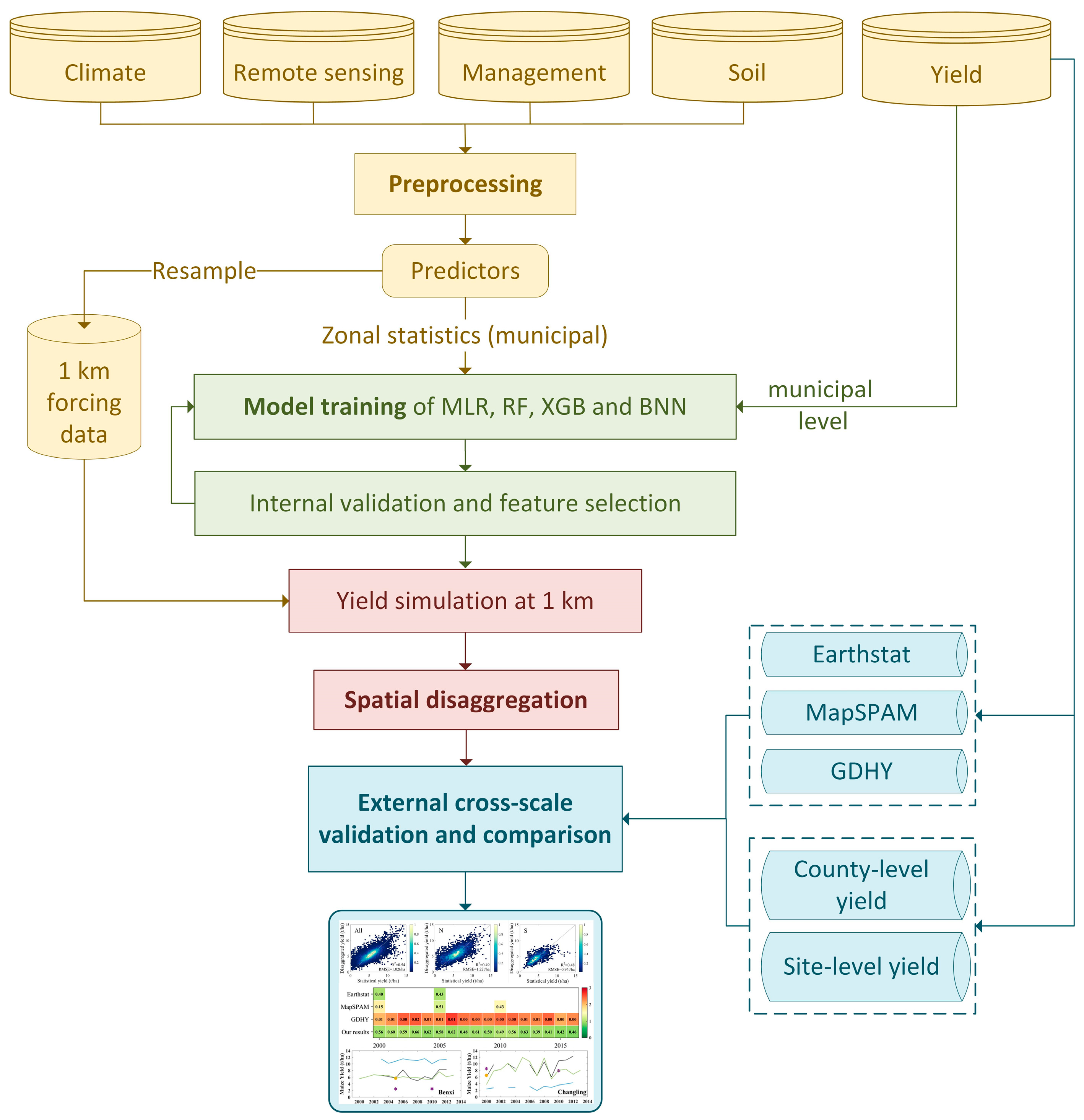
2.2.1. Preprocessing

Crop calendars recorded by stations were interpolated into grids using the nearest-neighbor interpolation method. The planting month was defined as month 1 to harmonize the order of months from planting, based on the planting and harvesting month of the crop calendars. The dynamic data whose temporal resolution was higher than monthly was composited into monthly and growing-seasonal predictors according to specific rules (

Table 1. Detailed information about the data collected in this work.

Dataset	Data Source	Original Resolution	Predictors	Description
Yield data	https://data.cnki.net/Yearbook/Navi?type=type&code=A (accessed on 8 May 2022)	Annual, 2000–2016 county and municipal-level	—	Yield
	China Meteorological Administration (https://data.cma.cn/, accessed on 8 May 2022)	Annual, 2000–2013 site level	—	Yield
	EarthStat [27]	5-year average, 2000 and 2005 10 km	—	Yield
	MapSPAM [37,65,66]	3-year average, 2000, 2005 and 2010 10 km	—	Yield
	GDHY [29]	Annual, 2000–2016 0.5°	—	Yield
Climate data	a 1-km monthly temperature and precipitation dataset for China from 1901 to 2017 [39]	Monthly, 2000–2016 1 km	Tmpm Tmpgs	Mean near-surface air temperature (TMP) for month m of the growing season (“gs”)
			Tmxm Tmxgs	Maximum near-surface air temperature
			Tmnm Tmngs	Minimum near-surface air temperature
			PREm PREgs	Total precipitation
	TerraClimate [40]	Monthly, 2000–2016 4 km	VPDm VPDgs	Mean vapor pressure deficit
			SRADm SRADgs	Mean downward shortwave flux at the surface
			PDSIm PDSIgs	Mean Palmer drought severity index
Remote sensing data	MYD11A2 and MOD11A2	8 day, 2000–2016 1 km	LSTDm LSTDgs	Maximum daytime land surface temperature
			LSTNm LSTNgs	Minimum nighttime land surface temperature
	MOD13A2	16 day, 2000–2016 1 km	NDVIm NDVIgs	Maximum normalized difference vegetation index
		16 day, 2000–2016 1 km	EVIm EVIgs	Maximum enhanced vegetation index
	CSIF [41]	16 day, 2000–2016 0.05°	SIFm SIFgs	Maximum solar-induced chlorophyll fluorescence
Management data	Fertilization [42]	Static, 2000 0.083°	NAT	Nitrogen application total
			PAT	Phosphorus application total
			KAT	Potassium application total
	—	Annual, 2000–2016	year	Prediction year
	Crop calendar (https://data.cma.cn/, accessed on 8 May 2022)	Annual, 2010–2013 site level	—	Planting and harvest months
	MapSPAM [37,65,66]	3-year average, 2000, 2005, and 2010 10 km	—	Harvest area
Soil data	HWSD [43]	Static, 2007 1 km	CEC_SOIL	Cation exchange capacity of soil
			CEC_CLAY	Cation exchange capacity of clay
			CLAY	Clay fraction
			OC	Percentage organic carbon
			pH	PH
			SAND	Sand fraction
			SILT	Silt fraction
	TerraClimate [40]	Monthly, 2000–2016 4 km	SMm SMgs	Mean soil moisture

Notes: “—”: not applicable; the subscript m stands for monthly values, while the subscript gs stands for growing-season values.

). For example, the maximum normalized difference vegetation index value was calculated monthly and by growing season, named “NDVI_m” and “NDVI_gs”, respectively; the data whose original temporal resolution was monthly were only composited to growing-seasonal predictors. For example, the average value of monthly mean near-surface air temperature during the growing season was calculated and named “TMP_gs.” Lastly, the SPAM maize harvest area was used as a mask to extract climate, remote sensing, management, and soil predictors. After that, predictors with various spatial resolutions were resampled to 1 km and then aggregated according to the municipal boundary for model training.

2.2.2. Model Training

Multivariate linear regression (MLR), random forest (RF), extreme gradient boosting (XGB), and Bayesian neural network (BNN) models were used to fit all of the municipal-year maize yield samples. MLR was conducted in this study to compare the above machine learning algorithms [67].

$$\ln Y=a_1{v}_1+\dots +a_n{v}_n+\epsilon$$

(1)

where Y is the municipal yield, $a_1,\dots ,a_n$ are the parameters to be fit, $v_1,\dots ,v_n$ are the predictors, and $\epsilon$ is the error term.

RF and XGB are both state-of-the-art tree-based ensemble methods that employ a collection of learning algorithms to achieve better predictive power than could be gained from any of these algorithms alone [68]. RF is a combination of tree predictors, such that each tree depends on the values of a random vector sampled independently and with the same distribution for all trees in the forest (Figure S3). The final predicted yield of RF is derived by averaging the predicted yields from all of the individual regression trees. The generalization error for forests converges to a limit as the number of trees in the forest becomes large. The generalization error of a forest of tree classifiers depends on the strength of the individual trees in the forest and the correlation between them [69]. XGB sequentially builds the model—adding a tree each time in XGB is fitting the residual of the previous prediction with a new function [70]. Unlike RF, each tree in XGB is fitted on a modified version of the original training dataset (Figure S4). XGB generalizes boosting methods by allowing the minimization of an arbitrary differentiable loss function; thus, it has a highly efficient realization of the gradient boosting and showed the best performance in recent machine learning challenges [71].

A BNN is a type of artificial neural network (ANN) that models the synapses in a biological brain, where the signal transmits from one neuron to another. The “signal” in ANNs is a real number, and the output of each neuron is calculated as the sum of its input according to specific nonlinear functions. The traditional ANNs need a considerable number of training samples to prevent the model from overfitting. However, BNNs introduce probability distributions over the weights in the neurons and are less prone to overfitting [72]. In this study, the BNN had an input layer with 256 neurons, two hidden layers with 128 neurons, and an output layer with two fully connected hidden layers, with 64 and 32 neurons each, respectively (Figure S5).

The MLR and RF models were trained using the LinearRegression and RandomForestRegressor modules from the package sklearn, while the XGB model was trained using XGBRegressor from the package xgboost in python. The BNN model was developed in TensorFlow 2.0 with Python version 3.7. To compare the performance of different models, the machine learning models were trained with default parameters. The default parameter values of RF and XGB can be found in Table S1, and more details about the settings of the BNN can be found in previous research [72]. To reveal the contribution of multisource data, the four models were driven by nine combinations of input data (

Table 2. The combinations of predictors.

Abbreviation	Predictors
c	Only climate predictors
r	Only remote sensing predictors
c + m	Climate and management predictors
r + m	Remote sensing and management predictors
c + s	Climate and soil predictors
r + s	Remote sensing and soil predictors
c + m + s	Climate, management, and soil predictors
r + m + s	Remote sensing, management, and soil predictors
c + r + m + s	Climate, remote sensing, management, and soil predictors

). Seventy-five percent of the complete dataset was randomly selected to train each model, and the remaining data were used to validate the model. The coefficient of determination (R²) and root-mean-square error (RMSE) between statistical and estimated yields were calculated to assess the predictive accuracy, according to Equations (2) and (3), respectively:

$$R^2=1-\frac{{\displaystyle \sum _{n=1}^N{(r_n-f_n)}^2}}{{\displaystyle \sum _{n=1}^N{(r_n-{\overline{r}}_n)}^2}},$$

(2)

$$RMSE=\sqrt{\frac{1}{N}{\displaystyle \sum _{n=1}^N{(r_n-f_n)}^2}}.$$

(3)

where $N$ is the number of samples, $r_n$ and $f_n$ refer to the municipal statistical yield and estimated maize yield, respectively, and ${\overline{r}}_n$ is the averages of $r_n$.

2.2.3. Spatial Disaggregation

After selecting the best-performing model, a leave-one-out method was adopted to identify the outliers, with estimated yields biased by more than three standard deviations relative to the observed yields [73]. The best-performing model was run using the default parameter values to identify the outliers (Table S1). The outlier elimination process can eliminate certain unrepresentative samples, which may introduce errors into the models [73,74,75]. Then, predictors with importance of over 1% were retained, according to feature importance in the scikit-learn module. Feature importance assesses how much each predictor decreases the weighted impurity. This procedure can effectively reduce the number of predictors, and further prevent models from overfitting the highly dimensional training data [76]. Lastly, the grid search was used to tune hyperparameters by trying all of the possible combinations of hyperparameter settings and comparing the out-of-bag data errors of the models with different combinations of parameters.

The gridded predictors at 1 km resolution were used to force the fine-tuned models and generate the gridded estimated yield of 2000–2016. Then, the estimated yield was used to compute the gridded distribution weight $w_{cit}$:

$$w_{cit}=\frac{y_{cit}^{sim}}{\frac{1}{I}{\displaystyle \sum _{i=1}^I{y}_{cit}^{sim}}},$$

(4)

where $y_{cit}^{sim}$ represents the estimated yield of the grid i located in the municipality c in the year t, and I is the number of grids located in this city. The weight $w_{cit}$ was then used to disaggregate the related statistical yield $Y_{ct}^{yb}$ to pixels. The disaggregated yield was produced by using the following equation:

$$y_{cit}=Y_{ct}^{yb}\cdot w_{cit}$$

(5)

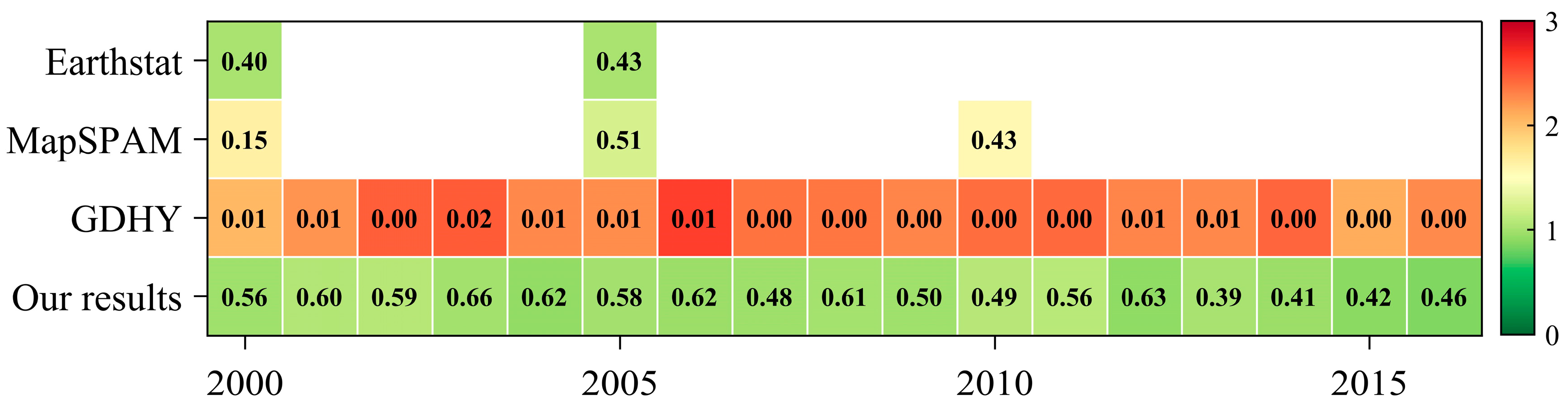
2.2.4. External Cross-Scale Validation

A common method to assess the accuracy of disaggregated yield is aggregating it to a finer spatial resolution and comparing it with statistical yield [12,37,77]. Such a procedure was conducted at the county level in this study. In addition, disaggregated yields were also validated using yield time-series from agrometeorological stations, which were superior to the cross-validation at the county level, but the number of agrometeorological stations was limited. For comparison purposes, the validation procedure included data from three existing global datasets: EarthStat, MapSPAM, and GDHY. We harmonized the temporal resolution to match different datasets to enable such a comparison. Our results were calculated to 5-year average yields in two periods—2000–2002 and 2003–2007 to compare with EarthStat. Three-year average yields of our results in three periods—2000–2001, 2004–2006, and 2009–2011—were calculated to match MapSPAM. For GDHY, the annual yields enable a year-to-year comparison. After that, the harmonized yield maps were aggregated to the county level, and comparisons were made with the county-level statistical yields. The R² and RMSE between statistical and disaggregated yields were calculated to assess the accuracy of gridded yield maps, according to Equations (2) and (3).

3. Results

3.1. Model Training Results

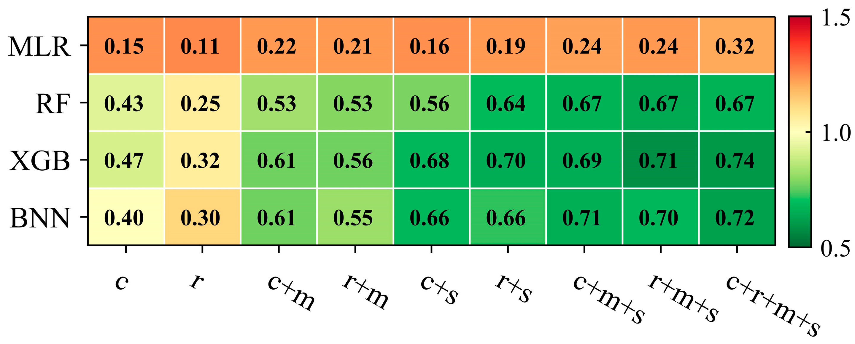
3.1.1. The Contribution of Machine Learning Approaches and Multisource Data

The model training statistics with various combinations of predictors and models are summarized in Figure 2. The machine learning models always outperformed the MLR. The XGB model showed better prediction skills than RF, and was comparable with the BNN. XGB showed a stronger ability than RF to integrate multisource data; the R² of XGB increased as more predictors were adopted, while the R² of RF reached the maximum (0.67) after integrating three types of predictors. The BNN outperformed XGB when it was driven by the combination of climate, management, and soil predictors, but XGB generally showed slight outperformance over the BNN when driven by other combinations.

Adding predictors tended to improve the models’ performance by increasing R² and reducing RMSE. If only one group of predictors was used, the climate predictors outperformed remote sensing predictors. Taking XGB as an example, the R² of the model with climate predictors was 0.47–0.15 greater than that of the model with remote sensing predictors only. When adding a second group of predictors, soil data improved model performance more than management data. The models generally had the highest accuracy forced by the full combination of multisource data (c + r + m + s). As the XGB model with a full list of predictors performed the best, we only present those results in the following sections. After parameter tuning, the R² between the estimated yields of XGB and the reported yields increased from 0.74 to 0.81 (Figure S6).

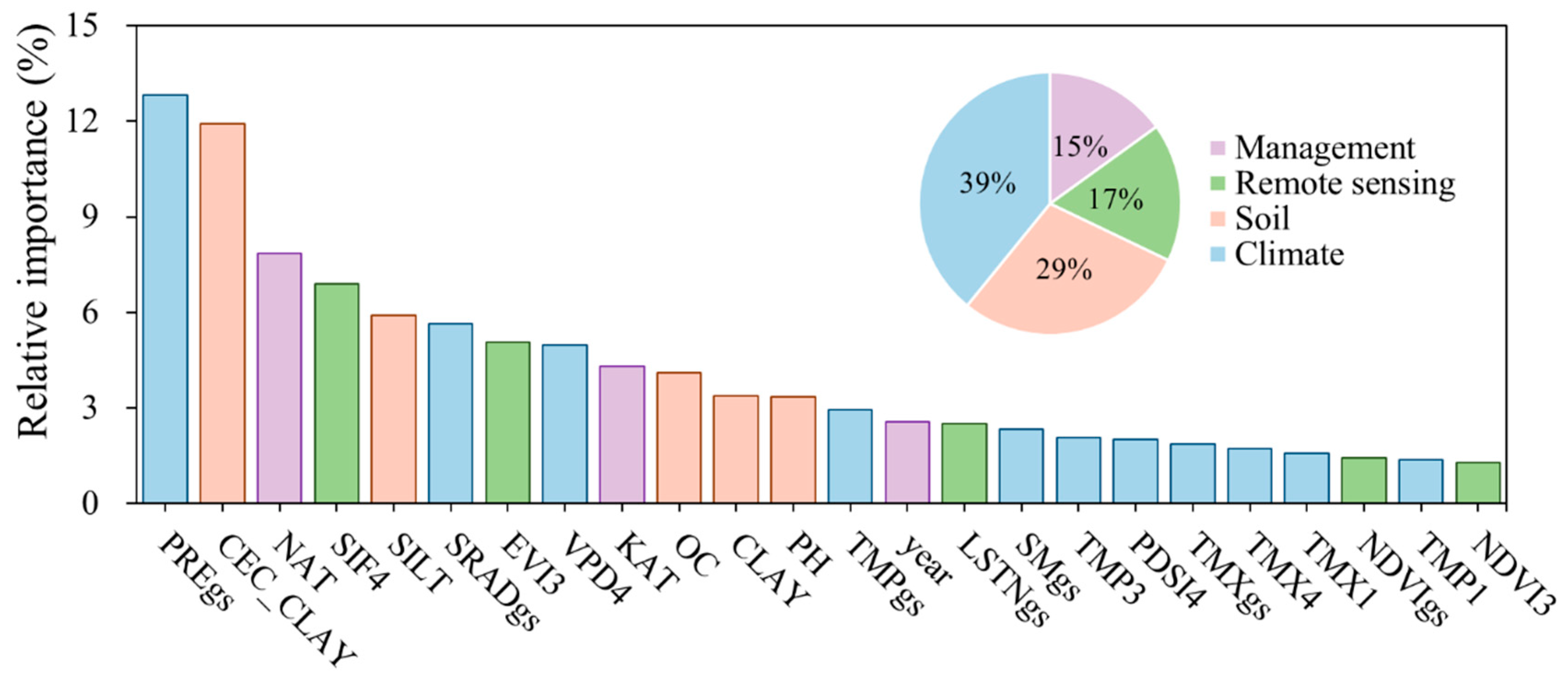
3.1.2. Feature Importance

The relative importance in maize yield prediction of climate, soil, remote-sensing, and management predictors was 39%, 29%, 17%, and 15%, respectively (Figure 3). There was a total of 23 predictors with relative importance greater than 1%. Among them, there were 10 climate predictors. Growing-season total precipitation (PREgs; 13%), the growing-season mean downward shortwave flux at the surface (SRADgs; 5.6%), and the fourth-month mean vapor pressure deficit (VPD4; 5%) were the top three climate predictors. Five soil predictors entered the final model, and the top three were the cation-exchange capacity of clay (CEC_CLAY), silt fraction (SILT), and percentage of organic carbon (OC), whose relative importance accounted for 12%, 5.9%, and 4.1%, respectively. There were four remote sensing predictors. Among them, the fourth-month maximum solar-induced chlorophyll fluorescence (SIF4) and third-month maximum enhanced vegetation index (EVI3) were the top two predictors. They made a relatively equal contribution to maize yield prediction, at 6.9% and 5.1%, respectively. There were three management predictors, among which the nitrogen application total (NAT) made the greatest relative contribution, at 7.9%.

3.2. Validation

3.2.1. Cross-Validation at the County Level

When cross-validated with the county-level statistical yield (Figure 4), our disaggregated yield can explain around 54% of the county-level yield variation in mainland China, with an RMSE of 1.02 t/ha. The gridded yield performed best in the Northern China maize zone and the Huang-Huai-Hai maize zone—two maize-planting zones. For regions with sparsely sown areas, it was more challenging to derive reasonable cross-validation scores, i.e., the northwestern maize zone.

Our method largely improved upon the accuracy of the gridded yield from the existing gridded maize yield datasets (Figure 5). Compared with EarthStat, the RMSE of our results was reduced by 16%, and the R² increased by around 0.13. Compared with MapSPAM, the RMSE of our results was reduced by 29–41%, and the R² increased by about 0.17, showing much better consistency with the statistical yields. Notably, there is a cutoff at 10 t/ha in MapSPAM2000, inconsistent with the statistical yields. Compared with GDHY, the improvement of our results was even greater than that of the previous two datasets. GDHY offered continuous annual yield series, but its R² was rather small (<0.02), and the RMSE was mostly greater than 2 t/ha.

3.2.2. Cross-Validation at the Site Level

In general, the yield series of our disaggregated results could capture the mean and interannual variation of the station records. Among the 99 sites (Table S2), the average R² of our results was 0.30, and the average RMSE was 2.39 t/ha, outperforming the other datasets. The only dataset with continuous yield was GDHY, and its average R² was 0.28, while its average RMSE was 3.17 t/ha. The RMSE of our results was 0.3 t/ha lower than that of EarthStat and 0.81 t/ha lower than that of MapSPAM for specific years. The yield series of the 24 best-documented sites are shown in Figure 6 and Figure S7. At most sites located in the major croplands, the yield series of our results (green lines) were much closer to the observations (black lines) than other yield datasets. However, in the minor corn-growing area, the capability of our method to capture the average and variability of maize yields was similar to that of other datasets, e.g., Qidong station in Jiangsu Province. In addition, there is a discontinuity in our results (green line) for Bachu station in 2009, because there were missing values in the remote sensing images.

4. Discussion

4.1. Machine Learning and Multisource Data Improved the Spatial Disaggregation Method

This study took advantage of multisource data and machine learning algorithms in yield prediction, and applied yield prediction results as spatial weights to disaggregate historical maize yield. Our cross-validation results indicated that the proposed method could reasonably generate spatiotemporally continuous gridded yields to large extents. This method benefits from two factors: first, the multisource data that contain rich information about maize growth and yield with various spatial resolutions, and second, the machine learning algorithm that could integrate the complicated relationships between these data.

Compared to our approach, existing spatial disaggregation methods mostly rely on only a few ancillary data, without considering the potential nonlinear and complex internal relationships. MapSPAM is another extreme case that uses a cross-entropy model to integrate multiple sources of information. Nevertheless, the MapSPAM predictors are fixed, and it is hard for researchers to explore the new sources of input information. Our cross-validation results indicate that our method could produce gridded data records slightly better than MapSPAM, and with higher flexibility.

Our method is promising in generating gridded yields at higher resolution because it can flexibly take more predictors with higher temporal and spatial resolution into account, while the spatial resolutions of existing datasets remain dominant at the 10–55 km level [26,27,37]. Our approach could readily be applied to disaggregate crop yields at various scales and resolutions. Most of the predictors used to generate weights in this study are available in the Google Earth Engine. National or subnational yield statistics can be collected from global agencies, including the Food and Agriculture Organization (FAO) and the World Bank.

Our method could be further improved by incorporating the machine learning model with process-based crop models such as the Agricultural Production Systems Simulator (APSIM) to predict maize yield grown in environments that have yet to be observed [72,78,79]. For example, we can expand the size of the training samples by simulating yield responses under different extreme environments on APSIM to help improve the generalizability of the machine learning model. A similar idea was adopted in the Scalable Crop Yield Mapper (SCYM) to estimate gridded yield in areas with few observational samples. The SCYM uses the pseudo-observations generated by APSIM as response variables and has achieved encouraging success in the USA and Africa [14,80,81].

4.2. Models’ Performance and Feature Importance in Maize Yield Prediction

In this study, we employed climate, remote sensing, soil, and management data. Our results indicated that their full combination was critical to providing complementary information in yield prediction. Among those four groups of predictors, climate predictors were the most relevant for maize yield in this study, because they provide background weather and external stressor information. However, our results greatly differed for individual climate predictors concerning the relative importance of precipitation and temperature. Growing-seasonal total precipitation (PREgs) was the most important predictor, while the contribution of growing-seasonal average temperature (TMPgs) was much smaller than that of precipitation (PREgs) here. This result is consistent with recent maize research conducted in Germany [82], but opposite conclusions were found in the Midwestern USA [61,72]. This may be because water stress has a stronger influence on maize yield than temperature stress in China, since more than 70% of the covered area affected by agrometeorological disasters was induced by drought or flood [83,84], and the very weak correlations between precipitation and yield in the USA may be the result of better irrigation conditions, larger irrigated areas, and more advanced equipment in the USA.

Soil predictors in our model ranked second in terms of contribution. However, soil predictors were less frequent in previous research, and their importance also remains controversial [53,64,72,85]. For instance, Crane-Droesch (2018) used 39 soil predictors for maize yield prediction, but found them to be the least important among climate, management, and soil predictors. A possible explanation for this disagreement centers around the homogeneity of soil in the US Corn Belt, in contrast with the huge heterogeneity in China. Our results highlight the importance of soil predictors—especially in China, whose arable areas show considerable heterogeneity. As for individual predictors, the cation exchange capacity of clay (CEC_CLAY) from this group ranked second among all of the predictors, consistent with conclusions from previous research conducted in the North China spring maize zone [53]. In addition, the contribution of soil moisture (SMgs) in this study was surprisingly limited, whereas it brought significant accuracy improvements to the process-based models in previous research [63,86,87,88]. This is because the soil moisture cannot reflect the physical damage and pollination disturbances caused by excessive rainfall in China. The soil moisture is also likely to become saturated under excessive rainfall; that is, although soil moisture can capture the influence of drought on maize yield, its ability to reflect conditions of excessive wetness is limited.

Remote sensing predictors were the third most important, because they contain unique information about the growing progress and health condition of crops [74]. The land surface temperature did not significantly outperform air temperature in our results, while previous research found that replacing air temperature with land surface temperature (LST) could significantly improve the model accuracy across the US Corn Belt [60]. However, Pede et al. (2019) only considered climate data and LST, while we used multisource data. Their research assumed that the LST can provide additional canopy information when using only climate data [89]. Our results indicated that this information might have been already captured by vegetation indices, such as the EVI.

Management predictors were the fourth most important, but the nitrogen application total (NAT) ranked third among all predictors. The dramatic increase in grain yield across the Chinese maize belt relied heavily on the application of nitrogen fertilizer [90], which can delay leaf senescence and sustain further grain yield increase—especially for high-yield maize production [91]. Although the application of fertilizer plays an important role in increasing grain yields in China [92,93,94], it has seldom been considered in yield prediction in previous research. Thus, our results encourage future studies to apply management predictors.

Machine learning models in this study highly outperformed MLR, due to MLR’s limitations in dealing with nonlinear relations and collinearity. Machine learning algorithms allow for the extraction of information about complicated interplays of various predictors, and can be performed independently from previously defined interrelationships [82,95]. The XGB model is comparable to the BNN, and similar results were found in previous research conducted in the USA and China [61,96]. This may be because it is hard to determine the optimal structure of a BNN, while the optimal parameters of XGB can be determined by cross-validation or grid search [96]. Furthermore, XGB showed better performance than RF, which is one of the most popular methods in yield prediction [33,53,61,97]. The superiority of XGB can be attributed to its boosting technique, which iteratively reduces bias and variance. Compared with RF, XGB fits each tree on a modified version of the original training dataset, i.e., every new tree uses information from previously grown trees [61].

4.3. Limitations and Future Work

This research is not free of uncertainties. First, our results could be significantly improved if we had access to the masks, which could present changes in the planting area from year to year. We only considered planting masks of 2000, 2005, and 2010 in this study due to lacking annual data, largely limiting the performance of our results. This problem will be solved as the cropland masks become increasingly available at high frequency and spatial resolution. Second, the generalization ability of machine learning models can be improved. For example, the XGB model trained at the municipal level succeeded in explaining around 81% of the municipal-level yield variation in the testing process (Figure S6), but only explained around 54% of the county-level yield variation (Figure 4). The weak generalization ability can be ascribed to the domain shift—the models trained from the municipal-level data may lose validity when directly applied to estimate yields at the gridded level, since they have different data distributions [98]. This problem will likely be addressed by integrating the process-based models or transfer learning [99,100,101,102].

5. Conclusions

This study developed a spatial disaggregation method based on machine learning algorithms and multisource data to produce spatially explicit gridded yields. Compared with the traditional disaggregation method, our method comprehensively considers the information contained in the multisource data, mining the relationships between them and maize yield through machine learning algorithms, while still maintaining strong flexibility and scalability. We found that XGB outperformed MLR and RF, and was comparable to the BNN. The disaggregated maps could reproduce 54% of the county-level yield variability when it was validated by finer-resolution statistical yields. The combination of machine learning and multisource data in producing spatially explicit yields improved upon the existing gridded datasets. Our method is not limited to using MODIS imagery as inputs, and shows promise in generating yield maps at much higher resolution and larger scales. Its accuracy could be further improved by transfer learning and integrating process-based models.

References

1. Hasegawa, T.; Sakurai, G.; Fujimori, S.; Takahashi, K.; Hijioka, Y.; Masui, T. Extreme Climate Events Increase Risk of Global Food Insecurity and Adaptation Needs. Nat. Food 2021, 2, 587–595. [Google Scholar] [CrossRef]
2. Jägermeyr, J.; Müller, C.; Ruane, A.C.; Elliott, J.; Balkovic, J.; Castillo, O.; Faye, B.; Foster, I.; Folberth, C.; Franke, J.A.; et al. Climate Impacts on Global Agriculture Emerge Earlier in New Generation of Climate and Crop Models. Nat. Food 2021, 2, 873–885. [Google Scholar] [CrossRef]
3. Stocker, T.F.; Qin, D.; Plattner, G.K.; Tignor, M.M.B.; Allen, S.K.; Boschung, J.; Nauels, A.; Xia, Y.; Bex, V.; Midgley, P.M. Climate Change 2013 the Physical Science Basis: Working Group I Contribution to the Fifth Assessment Report of the Intergovernmental Panel on Climate Change; Cambridge University Press: New York, NY, USA, 2013; ISBN 978-1-107-05799-9. [Google Scholar]
4. Zhao, C.; Liu, B.; Piao, S.; Wang, X.; Lobell, D.B.; Huang, Y.; Huang, M.; Yao, Y.; Bassu, S.; Ciais, P.; et al. Temperature Increase Reduces Global Yields of Major Crops in Four Independent Estimates. Proc. Natl. Acad. Sci. USA 2017, 114, 9326–9331. [Google Scholar] [CrossRef] [PubMed] [Green Version]
5. Liu, B.; Asseng, S.; Müller, C.; Ewert, F.; Elliott, J.; Lobell, D.B.; Martre, P.; Ruane, A.C.; Wallach, D.; Jones, J.W.; et al. Similar Estimates of Temperature Impacts on Global Wheat Yield by Three Independent Methods. Nat. Clim. Chang. 2016, 6, 1130–1136. [Google Scholar] [CrossRef]
6. Asseng, S.; Ewert, F.; Martre, P.; Rötter, R.P.; Lobell, D.B.; Cammarano, D.; Kimball, B.A.; Ottman, M.J.; Wall, G.W.; White, J.W.; et al. Rising Temperatures Reduce Global Wheat Production. Nat. Clim. Chang. 2015, 5, 143–147. [Google Scholar] [CrossRef]
7. Wang, X.; Zhao, C.; Müller, C.; Wang, C.; Ciais, P.; Janssens, I.; Peñuelas, J.; Asseng, S.; Li, T.; Elliott, J.; et al. Emergent Constraint on Crop Yield Response to Warmer Temperature from Field Experiments. Nat. Sustain. 2020, 3, 908–916. [Google Scholar] [CrossRef]
8. Yu, Q.; Wu, W.; Yang, P.; Li, Z.; Xiong, W.; Tang, H. Proposing an Interdisciplinary and Cross-Scale Framework for Global Change and Food Security Researches. Agric. Ecosyst. Environ. 2012, 156, 57–71. [Google Scholar] [CrossRef]
9. Ojeda, J.J.; Rezaei, E.E.; Remenyi, T.A.; Webber, H.A.; Siebert, S.; Meinke, H.; Webb, M.A.; Kamali, B.; Harris, R.M.B.; Kidd, D.B.; et al. Implications of Data Aggregation Method on Crop Model Outputs—The Case of Irrigated Potato Systems in Tasmania, Australia. Eur. J. Agron. 2021, 126, 126276. [Google Scholar] [CrossRef]
10. Angulo, C.; Gaiser, T.; Rötter, R.P.; Børgesen, C.D.; Hlavinka, P.; Trnka, M.; Ewert, F. “Fingerprints” of Four Crop Models as Affected by Soil Input Data Aggregation. Eur. J. Agron. 2014, 61, 35–48. [Google Scholar] [CrossRef]
11. Claassen, R.; Just, R.E. Heterogeneity and Distributional form of Farm-Level Yields. Am. J. Agric. Econ. 2011, 93, 144–160. [Google Scholar] [CrossRef] [Green Version]
12. Iizumi, T.; Yokozawa, M.; Sakurai, G.; Travasso, M.I.; Romanernkov, V.; Oettli, P.; Newby, T.; Ishigooka, Y.; Furuya, J. Historical Changes in Global Yields: Major Cereal and Legume Crops from 1982 to 2006. Glob. Ecol. Biogeogr. 2014, 23, 346–357. [Google Scholar] [CrossRef]
13. Lobell, D.B. The Use of Satellite Data for Crop Yield Gap Analysis. Field Crop. Res. 2013, 143, 56–64. [Google Scholar] [CrossRef] [Green Version]
14. Jin, Z.; Azzari, G.; Lobell, D.B. Improving the Accuracy of Satellite-Based High-Resolution Yield Estimation: A Test of Multiple Scalable Approaches. Agric. For. Meteorol. 2017, 247, 207–220. [Google Scholar] [CrossRef]
15. Diker, K.; Heermann, D.F.; Brodahl, M.K. Frequency Analysis of Yield for Delineating Yield Response Zones. Precis. Agric. 2004, 5, 435–444. [Google Scholar] [CrossRef]
16. Liu, W.; Ye, T.; Jagermeyr, J.; Müller, C.; Chen, S.; Liu, X.; Shi, P. Future Climate Change Significantly Alters Interannual Wheat Yield Variability over Half of Harvested Areas. Environ. Res. Lett. 2021, 16, 094045. [Google Scholar] [CrossRef]
17. Xu, Y.; Chou, J.; Yang, F.; Sun, M.; Zhao, W.; Li, J. Article Assessing the Sensitivity of Main Crop Yields to Climate Change Impacts in China. Atmosphere 2021, 12, 172. [Google Scholar] [CrossRef]
18. Wu, J.-Z.; Zhang, J.; Ge, Z.-M.; Xing, L.-W.; Han, S.-Q.; Shen, C.; Kong, F.-T. Impact of Climate Change on Maize Yield in China from 1979 to 2016. J. Integr. Agric. 2021, 20, 289–299. [Google Scholar] [CrossRef]
19. Piao, S.; Ciais, P.; Huang, Y.; Shen, Z.; Peng, S.; Li, J.; Zhou, L.; Liu, H.; Ma, Y.; Ding, Y.; et al. The Impacts of Climate Change on Water Resources and Agriculture in China. Nature 2010, 467, 43–51. [Google Scholar] [CrossRef]
20. Shi, W.; Wang, M.; Liu, Y. Crop Yield and Production Responses to Climate Disasters in China. Sci. Total Environ. 2021, 750, 141147. [Google Scholar] [CrossRef]
21. Chen, C.; Baethgen, W.E.; Wang, E.; Yu, Q. Characterizing Spatial and Temporal Variability of Crop Yield Caused by Climate and Irrigation in the North China Plain. Theor. Appl. Climatol. 2011, 106, 365–381. [Google Scholar] [CrossRef]
22. Li, X.; Fang, S.; Wu, D.; Zhu, Y.; Wu, Y. Risk Analysis of Maize Yield Losses in Mainland China at the County Level. Sci. Rep. 2020, 10, 10684. [Google Scholar] [CrossRef] [PubMed]
23. Kim, K.H.; Doi, Y.; Ramankutty, N.; Iizumi, T. A Review of Global Gridded Cropping System Data Products. Environ. Res. Lett. 2021, 16, 093005. [Google Scholar] [CrossRef]
24. Joglekar, A.K.B.; Wood-Sichra, U.; Pardey, P.G. Pixelating Crop Production: Consequences of Methodological Choices. PLoS ONE 2019, 14, e0212281. [Google Scholar] [CrossRef] [PubMed]
25. Portmann, F.T.; Siebert, S.; Döll, P. MIRCA2000-Global Monthly Irrigated and Rainfed Crop Areas around the Year 2000: A New High-Resolution Data Set for Agricultural and Hydrological Modeling. Glob. Biogeochem. Cycles 2010, 24, GB1011. [Google Scholar] [CrossRef]
26. Monfreda, C.; Ramankutty, N.; Foley, J.A. Farming the Planet: 2. Geographic Distribution of Crop Areas, Yields, Physiological Types, and Net Primary Production in the Year 2000. Glob. Biogeochem. Cycles 2008, 22, 1–19. [Google Scholar] [CrossRef]
27. Ray, D.K.; Ramankutty, N.; Mueller, N.D.; West, P.C.; Foley, J.A. Recent Patterns of Crop Yield Growth and Stagnation. Nat. Commun. 2012, 3, 1293. [Google Scholar] [CrossRef] [Green Version]
28. Szyniszewska, A.M. CassavaMap, a Fine-Resolution Disaggregation of Cassava Production and Harvested Area in Africa in 2014. Sci. Data 2020, 7, 159. [Google Scholar] [CrossRef]
29. Iizumi, T.; Sakai, T. The Global Dataset of Historical Yields for Major Crops 1981–2016. Sci. Data 2020, 7, 97. [Google Scholar] [CrossRef] [Green Version]
30. Zhang, L.; Zhang, Z.; Luo, Y.; Cao, J.; Xie, R.; Li, S. Integrating Satellite-Derived Climatic and Vegetation Indices to Predict Smallholder Maize Yield Using Deep Learning. Agric. For. Meteorol. 2021, 311, 108666. [Google Scholar] [CrossRef]
31. Cao, J.; Zhang, Z.; Tao, F.; Zhang, L.; Luo, Y.; Zhang, J.; Han, J.; Xie, J. Integrating Multi-Source Data for Rice Yield Prediction across China Using Machine Learning and Deep Learning Approaches. Agric. For. Meteorol. 2021, 297, 108275. [Google Scholar] [CrossRef]
32. Cai, Y.; Guan, K.; Lobell, D.; Potgieter, A.B.; Wang, S.; Peng, J.; Xu, T.; Asseng, S.; Zhang, Y.; You, L.; et al. Integrating Satellite and Climate Data to Predict Wheat Yield in Australia Using Machine Learning Approaches. Agric. For. Meteorol. 2019, 274, 144–159. [Google Scholar] [CrossRef]
33. Schwalbert, R.A.; Amado, T.; Corassa, G.; Pott, L.P.; Prasad, P.V.V.; Ciampitti, I.A. Satellite-Based Soybean Yield Forecast: Integrating Machine Learning and Weather Data for Improving Crop Yield Prediction in Southern Brazil. Agric. For. Meteorol. 2020, 284, 107886. [Google Scholar] [CrossRef]
34. Yang, Y.; Anderson, M.C.; Gao, F.; Johnson, D.M.; Yang, Y.; Sun, L.; Dulaney, W.; Hain, C.R.; Otkin, J.A.; Prueger, J.; et al. Phenological Corrections to a Field-Scale, ET-Based Crop Stress Indicator: An Application to Yield Forecasting across the U.S. Corn Belt. Remote Sens. Environ. 2021, 257, 112337. [Google Scholar] [CrossRef]
35. Hunt, M.L.; Blackburn, G.A.; Carrasco, L.; Redhead, J.W.; Rowland, C.S. High Resolution Wheat Yield Mapping Using Sentinel-2. Remote Sens. Environ. 2019, 233, 111410. [Google Scholar] [CrossRef]
36. Kang, Y.; Özdoğan, M. Field-Level Crop Yield Mapping with Landsat Using a Hierarchical Data Assimilation Approach. Remote Sens. Environ. 2019, 228, 144–163. [Google Scholar] [CrossRef]
37. Yu, Q.; You, L.; Wood-Sichra, U.; Ru, Y.; Joglekar, A.K.B.; Fritz, S.; Xiong, W.; Lu, M.; Wu, W.; Yang, P. A Cultivated Planet in 2010—Part 2: The Global Gridded Agricultural-Production Maps. Earth Syst. Sci. Data 2020, 12, 3545–3572. [Google Scholar] [CrossRef]
38. Iizumi, T.; Kotoku, M.; Kim, W.; West, P.C.; Gerber, J.S.; Id, M.E.B. Uncertainties of Potentials and Recent Changes in Global Yields of Major Crops Resulting from Census- and Satellite-Based Yield Datasets at Multiple Resolutions. PLoS ONE 2018, 13, e0203809. [Google Scholar] [CrossRef]
39. Peng, S.; Ding, Y.; Liu, W.; Li, Z. 1 Km Monthly Temperature and Precipitation Dataset for China from 1901 to 2017. Earth Syst. Sci. Data 2019, 11, 1931–1946. [Google Scholar] [CrossRef] [Green Version]
40. Abatzoglou, J.T.; Dobrowski, S.Z.; Parks, S.A.; Hegewisch, K.C. TerraClimate, a High-Resolution Global Dataset of Monthly Climate and Climatic Water Balance from 1958–2015. Sci. Data 2018, 5, 170191. [Google Scholar] [CrossRef] [Green Version]
41. Zhang, Y.; Joiner, J.; Alemohammad, S.H.; Zhou, S.; Gentine, P. A Global Spatially Contiguous Solar-Induced Fluorescence (CSIF) Dataset Using Neural Networks. Biogeosciences 2018, 15, 5779–5800. [Google Scholar] [CrossRef] [Green Version]
42. Mueller, N.D.; Gerber, J.S.; Johnston, M.; Ray, D.K.; Ramankutty, N.; Foley, J.A. Closing Yield Gaps through Nutrient and Water Management. Nature 2012, 490, 254–257. [Google Scholar] [CrossRef]
43. Sugawara, E.; Nikaido, H. Properties of AdeABC and AdeIJK Efflux Systems of Acinetobacter Baumannii Compared with Those of the AcrAB-TolC System of Escherichia Coli. Antimicrob. Agents Chemother. 2014, 58, 7250–7257. [Google Scholar] [CrossRef] [PubMed] [Green Version]
44. Cane, M.A.; Eshel, G.; Buckland, R.W. Forecasting Zimbabwean Maize Yield Using Eastern Equatorial Pacific Sea Surface Temperature. Nature 1994, 370, 204–205. [Google Scholar] [CrossRef]
45. Soler, C.M.T.; Sentelhas, P.C.; Hoogenboom, G. Application of the CSM-CERES-Maize Model for Planting Date Evaluation and Yield Forecasting for Maize Grown off-Season in a Subtropical Environment. Eur. J. Agron. 2007, 27, 165–177. [Google Scholar] [CrossRef]
46. Gao, Y.; Wang, S.; Guan, K.; Wolanin, A.; You, L.; Ju, W.; Zhang, Y. The Ability of Sun-Induced Chlorophyll Fluorescence from OCO-2 and MODIS-EVI to Monitor Spatial Variations of Soybean and Maize Yields in the Midwestern USA. Remote Sens. 2020, 12, 1111. [Google Scholar] [CrossRef] [Green Version]
47. Lobell, D.B.; Roberts, M.J.; Schlenker, W.; Braun, N.; Little, B.B.; Rejesus, R.M.; Hammer, G.L. Greater Sensitivity to Drought Accompanies Maize Yield Increase in the U.S. Midwest. Science 2014, 344, 516–519. [Google Scholar] [CrossRef] [PubMed]
48. Peng, B.; Guan, K.; Pan, M.; Li, Y. Benefits of Seasonal Climate Prediction and Satellite Data for Forecasting U.S. Maize Yield. Geophys. Res. Lett. 2018, 45, 9662–9671. [Google Scholar] [CrossRef]
49. Schlenker, W.; Roberts, M.J. Nonlinear Temperature Effects Indicate Severe Damages to U.S. Crop Yields under Climate Change. Proc. Natl. Acad. Sci. USA 2009, 106, 15594–15598. [Google Scholar] [CrossRef] [Green Version]
50. Peña-Gallardo, M.; Vicente-Serrano, S.M.; Quiring, S.; Svoboda, M.; Hannaford, J.; Tomas-Burguera, M.; Martín-Hernández, N.; Domínguez-Castro, F.; El Kenawy, A. Response of Crop Yield to Different Time-Scales of Drought in the United States: Spatio-Temporal Patterns and Climatic and Environmental Drivers. Agric. For. Meteorol. 2019, 264, 40–55. [Google Scholar] [CrossRef] [Green Version]
51. Mkhabela, M.S.; Mkhabela, M.S.; Mashinini, N.N. Early Maize Yield Forecasting in the Four Agro-Ecological Regions of Swaziland Using NDVI Data Derived from NOAA’s-AVHRR. Agric. For. Meteorol. 2005, 129, 1–9. [Google Scholar] [CrossRef]
52. Nagy, A.; Fehér, J.; Tamás, J. Wheat and Maize Yield Forecasting for the Tisza River Catchment Using MODIS NDVI Time Series and Reported Crop Statistics. Comput. Electron. Agric. 2018, 151, 41–49. [Google Scholar] [CrossRef]
53. Zhang, L.; Zhang, Z.; Luo, Y.; Cao, J.; Tao, F. Combining Optical, Fluorescence, Thermal Satellite, and Environmental Data to Predict County-Level Maize Yield in China Using Machine Learning Approaches. Remote Sens. 2020, 12, 21. [Google Scholar] [CrossRef] [Green Version]
54. Johnson, D.M. An Assessment of Pre- and within-Season Remotely Sensed Variables for Forecasting Corn and Soybean Yields in the United States. Remote Sens. Environ. 2014, 141, 116–128. [Google Scholar] [CrossRef]
55. Bolton, D.K.; Friedl, M.A. Forecasting Crop Yield Using Remotely Sensed Vegetation Indices and Crop Phenology Metrics. Agric. For. Meteorol. 2013, 173, 74–84. [Google Scholar] [CrossRef]
56. Somkuti, P.; Bösch, H.; Feng, L.; Palmer, P.I.; Parker, R.J.; Quaife, T. A New Space-Borne Perspective of Crop Productivity Variations over the US Corn Belt. Agric. For. Meteorol. 2020, 281, 107826. [Google Scholar] [CrossRef]
57. Song, L.; Guanter, L.; Guan, K.; You, L.; Huete, A.; Ju, W.; Zhang, Y. Satellite Sun-Induced Chlorophyll Fluorescence Detects Early Response of Winter Wheat to Heat Stress in the Indian Indo-Gangetic Plains. Glob. Chang. Biol. 2018, 24, 4023–4037. [Google Scholar] [CrossRef] [Green Version]
58. Kimm, H.; Guan, K.; Burroughs, C.H.; Peng, B.; Ainsworth, E.A.; Bernacchi, C.J.; Moore, C.E.; Kumagai, E.; Yang, X.; Berry, J.A.; et al. Quantifying High-Temperature Stress on Soybean Canopy Photosynthesis: The Unique Role of Sun-Induced Chlorophyll Fluorescence. Glob. Chang. Biol. 2021, 27, 2403–2415. [Google Scholar] [CrossRef]
59. Johnson, D.M. A Comprehensive Assessment of the Correlations between Field Crop Yields and Commonly Used MODIS Products. Int. J. Appl. Earth Obs. Geoinf. 2016, 52, 65–81. [Google Scholar] [CrossRef] [Green Version]
60. Pede, T.; Mountrakis, G.; Shaw, S.B. Improving Corn Yield Prediction across the US Corn Belt by Replacing Air Temperature with Daily MODIS Land Surface Temperature. Agric. For. Meteorol. 2019, 276–277, 107615. [Google Scholar] [CrossRef]
61. Kang, Y.; Ozdogan, M.; Zhu, X.; Ye, Z.; Hain, C.; Anderson, M. Comparative Assessment of Environmental Variables and Machine Learning Algorithms for Maize Yield Prediction in the US Midwest. Environ. Res. Lett. 2020, 15, 045023. [Google Scholar] [CrossRef]
62. Zhao, J.; Yang, X.; Sun, S. Constraints on Maize Yield and Yield Stability in the Main Cropping Regions in China. Eur. J. Agron. 2018, 99, 106–115. [Google Scholar] [CrossRef]
63. Ines, A.V.M.; Das, N.N.; Hansen, J.W.; Njoku, E.G. Assimilation of Remotely Sensed Soil Moisture and Vegetation with a Crop Simulation Model for Maize Yield Prediction. Remote Sens. Environ. 2013, 138, 149–164. [Google Scholar] [CrossRef] [Green Version]
64. Khaki, S.; Wang, L. Crop Yield Prediction Using Deep Neural Networks. Front. Plant Sci. 2019, 10, 1–10. [Google Scholar] [CrossRef] [PubMed] [Green Version]
65. You, L.; Wood, S. An Entropy Approach to Spatial Disaggregation of Agricultural Production. Agric. Syst. 2006, 90, 329–347. [Google Scholar] [CrossRef]
66. You, L.; Wood, S.; Wood-Sichra, U.; Wu, W. Generating Global Crop Distribution Maps: From Census to Grid. Agric. Syst. 2014, 127, 53–60. [Google Scholar] [CrossRef] [Green Version]
67. Lobell, D.B.; Burke, M.B. On the Use of Statistical Models to Predict Crop Yield Responses to Climate Change. Agric. For. Meteorol. 2010, 150, 1443–1452. [Google Scholar] [CrossRef]
68. Folberth, C.; Baklanov, A.; Balkovič, J.; Skalský, R.; Khabarov, N.; Obersteiner, M. Spatio-Temporal Downscaling of Gridded Crop Model Yield Estimates Based on Machine Learning. Agric. For. Meteorol. 2019, 264, 1–15. [Google Scholar] [CrossRef] [Green Version]
69. Breiman, L. Random Forests. Mach. Learn. 2001, 45, 5–32. [Google Scholar] [CrossRef] [Green Version]
70. Guo, R.; Zhao, Z.; Wang, T.; Liu, G.; Zhao, J.; Gao, D. Degradation State Recognition of Piston Pump Based on ICEEMDAN and XGBoost. Appl. Sci. 2020, 10, 6593. [Google Scholar] [CrossRef]
71. Chen, T.; Guestrin, C. XGBoost: A Scalable Tree Boosting System. In KDD’16, Proceedings of the 22nd ACM SIGKDD International Conference on Knowledge Discovery and Data Mining, Online Conference, 13 August 2016; ACM: New York, NY, USA, 2016; pp. 785–794. [Google Scholar] [CrossRef] [Green Version]
72. Ma, Y.; Zhang, Z.; Kang, Y.; Özdoğan, M. Corn Yield Prediction and Uncertainty Analysis Based on Remotely Sensed Variables Using a Bayesian Neural Network Approach. Remote Sens. Environ. 2021, 259, 112408. [Google Scholar] [CrossRef]
73. Li, W.; Ciais, P.; Stehfest, E.; van Vuuren, D.; Popp, A.; Arneth, A.; Di Fulvio, F.; Doelman, J.; Humpenöder, F.; Harper, A.B.; et al. Mapping the Yields of Lignocellulosic Bioenergy Crops from Observations at the Global Scale. Earth Syst. Sci. Data 2020, 12, 789–804. [Google Scholar] [CrossRef] [Green Version]
74. Tramontana, G.; Ichii, K.; Camps-Valls, G.; Tomelleri, E.; Papale, D. Uncertainty Analysis of Gross Primary Production Upscaling Using Random Forests, Remote Sensing and Eddy Covariance Data. Remote Sens. Environ. 2015, 168, 360–373. [Google Scholar] [CrossRef]
75. Siewert, M.B. High-Resolution Digital Mapping of Soil Organic Carbon in Permafrost Terrain Using Machine Learning: A Case Study in a Sub-Arctic Peatland Environment. Biogeosciences 2018, 15, 1663–1682. [Google Scholar] [CrossRef] [Green Version]
76. Shahhosseini, M.; Hu, G.; Huber, I.; Archontoulis, S.V. Coupling Machine Learning and Crop Modeling Improves Crop Yield Prediction in the US Corn Belt. Sci. Rep. 2021, 11, 1606. [Google Scholar] [CrossRef]
77. Ye, T.; Zhao, N.; Yang, X.; Ouyang, Z.; Liu, X.; Chen, Q.; Hu, K.; Yue, W.; Qi, J.; Li, Z.; et al. Improved Population Mapping for China Using Remotely Sensed and Points-of-Interest Data within a Random Forests Model. Sci. Total Environ. 2019, 658, 936–946. [Google Scholar] [CrossRef]
78. Bassu, S.; Brisson, N.; Durand, J.L.; Boote, K.; Lizaso, J.; Jones, J.W.; Rosenzweig, C.; Ruane, A.C.; Adam, M.; Baron, C.; et al. How Do Various Maize Crop Models Vary in Their Responses to Climate Change Factors? Glob. Chang. Biol. 2014, 20, 2301–2320. [Google Scholar] [CrossRef]
79. Lobell, D.B.; Hammer, G.L.; McLean, G.; Messina, C.; Roberts, M.J.; Schlenker, W. The Critical Role of Extreme Heat for Maize Production in the United States. Nat. Clim. Chang. 2013, 3, 497–501. [Google Scholar] [CrossRef]
80. Jin, Z.; Azzari, G.; You, C.; Di Tommaso, S.; Aston, S.; Burke, M.; Lobell, D.B. Smallholder Maize Area and Yield Mapping at National Scales with Google Earth Engine. Remote Sens. Environ. 2019, 228, 115–128. [Google Scholar] [CrossRef]
81. Lobell, D.B.; Thau, D.; Seifert, C.; Engle, E.; Little, B. A Scalable Satellite-Based Crop Yield Mapper. Remote Sens. Environ. 2015, 164, 324–333. [Google Scholar] [CrossRef]
82. Lischeid, G.; Webber, H.; Sommer, M.; Nendel, C.; Ewert, F. Machine Learning in Crop Yield Modelling: A Powerful Tool, but No Surrogate for Science. Agric. For. Meteorol. 2022, 312, 108698. [Google Scholar] [CrossRef]
83. Xu, X.; Tang, Q. Spatiotemporal Variations in Damages to Cropland from Agrometeorological Disasters in Mainland China during 1978–2018. Sci. Total Environ. 2021, 785, 147247. [Google Scholar] [CrossRef] [PubMed]
84. Ye, T.; Shi, P.; Wang, J.; Liu, L.; Fan, Y.; Hu, J. China’s Drought Disaster Risk Management: Perspective of Severe Droughts in 2009–2010. Int. J. Disaster Risk Sci. 2012, 3, 84–97. [Google Scholar] [CrossRef] [Green Version]
85. Crane-Droesch, A. Machine Learning Methods for Crop Yield Prediction and Climate Change Impact Assessment in Agriculture. Environ. Res. Lett. 2018, 13, 114003. [Google Scholar] [CrossRef] [Green Version]
86. De Wit, A.J.W.; van Diepen, C.A. Crop Model Data Assimilation with the Ensemble Kalman Filter for Improving Regional Crop Yield Forecasts. Agric. For. Meteorol. 2007, 146, 38–56. [Google Scholar] [CrossRef]
87. Mishra, V.; Cruise, J.F.; Mecikalski, J.R. Assimilation of Coupled Microwave/Thermal Infrared Soil Moisture Profiles into a Crop Model for Robust Maize Yield Estimates over Southeast United States. Eur. J. Agron. 2021, 123, 126208. [Google Scholar] [CrossRef]
88. Pauwels, V.R.N.; Verhoest, N.E.C.; de Lannoy, G.J.M.; Guissard, V.; Lucau, C.; Defourny, P. Optimization of a Coupled Hydrology-Crop Growth Model through the Assimilation of Observed Soil Moisture and Leaf Area Index Values Using an Ensemble Kalman Filter. Water Resour. Res. 2007, 43, 1–17. [Google Scholar] [CrossRef] [Green Version]
89. Heft-Neal, S.; Lobell, D.B.; Burke, M. Using Remotely Sensed Temperature to Estimate Climate Response Functions. Environ. Res. Lett. 2017, 12, 014013. [Google Scholar] [CrossRef] [Green Version]
90. Chen, X.P.; Cui, Z.L.; Vitousek, P.M.; Cassman, K.G.; Matson, P.A.; Bai, J.S.; Meng, Q.F.; Hou, P.; Yue, S.C.; Römheld, V.; et al. Integrated Soil-Crop System Management for Food Security. Proc. Natl. Acad. Sci. USA 2011, 108, 6399–6404. [Google Scholar] [CrossRef] [Green Version]
91. Hou, P.; Gao, Q.; Xie, R.; Li, S.; Meng, Q.; Kirkby, E.A.; Römheld, V.; Müller, T.; Zhang, F.; Cui, Z.; et al. Grain Yields in Relation to N Requirement: Optimizing Nitrogen Management for Spring Maize Grown in China. Field Crop. Res. 2012, 129, 1–6. [Google Scholar] [CrossRef]
92. Xu, X.; He, P.; Zhang, J.; Pampolino, M.F.; Johnston, A.M.; Zhou, W. Spatial Variation of Attainable Yield and Fertilizer Requirements for Maize at the Regional Scale in China. Field Crop. Res. 2017, 203, 8–15. [Google Scholar] [CrossRef]
93. Qiu, S.; Xie, J.; Zhao, S.; Xu, X.; Hou, Y.; Wang, X.; Zhou, W.; He, P.; Johnston, A.M.; Christie, P.; et al. Long-Term Effects of Potassium Fertilization on Yield, Efficiency, and Soil Fertility Status in a Rain-Fed Maize System in Northeast China. Field Crop. Res. 2014, 163, 1–9. [Google Scholar] [CrossRef]
94. Qiu, S.J.; He, P.; Zhao, S.C.; Li, W.J.; Xie, J.G.; Hou, Y.P.; Grant, C.A.; Zhou, W.; Jin, J.Y. Impact of Nitrogen Rate on Maize Yield and Nitrogen Use Efficiencies in Northeast China. Agron. J. 2015, 107, 305–313. [Google Scholar] [CrossRef]
95. Hoffman, A.L.; Kemanian, A.R.; Forest, C.E. Analysis of Climate Signals in the Crop Yield Record of Sub-Saharan Africa. Glob. Chang. Biol. 2018, 24, 143–157. [Google Scholar] [CrossRef] [PubMed]
96. Xu, H.; Zhang, X.; Ye, Z.; Jiang, L.; Qiu, X.; Tian, Y.; Zhu, Y.; Cao, W. Machine Learning Approaches Can Reduce Environmental Data Requirements for Regional Yield Potential Simulation. Eur. J. Agron. 2021, 129, 126335. [Google Scholar] [CrossRef]
97. Huang, X.; Xiao, J.; Wang, X.; Ma, M. Improving the Global MODIS GPP Model by Optimizing Parameters with FLUXNET Data. Agric. For. Meteorol. 2021, 300, 108314. [Google Scholar] [CrossRef]
98. Kouw, W.M.; Loog, M. A Review of Domain Adaptation without Target Labels. IEEE Trans. Pattern Anal. Mach. Intell. 2021, 43, 766–785. [Google Scholar] [CrossRef] [PubMed] [Green Version]
99. Wang, A.X.; Tran, C.; Desai, N.; Lobell, D.; Ermon, S. Deep Transfer Learning for Crop Yield Prediction with Remote Sensing Data. In Proceedings of the 1st ACM SIGCAS Conference on Computing and Sustainable Societies, Online Conference, 20–22 June 2018. [Google Scholar] [CrossRef]
100. Ma, Y.; Zhang, Z.; Yang, H.L.; Yang, Z. An Adaptive Adversarial Domain Adaptation Approach for Corn Yield Prediction. Comput. Electron. Agric. 2021, 187, 106314. [Google Scholar] [CrossRef]
101. Chen, J.; Chen, J.; Zhang, D.; Sun, Y.; Nanehkaran, Y.A. Using Deep Transfer Learning for Image-Based Plant Disease Identification. Comput. Electron. Agric. 2020, 173, 105393. [Google Scholar] [CrossRef]
102. Barbedo, J.G.A. Impact of Dataset Size and Variety on the Effectiveness of Deep Learning and Transfer Learning for Plant Disease Classification. Comput. Electron. Agric. 2018, 153, 46–53. [Google Scholar] [CrossRef]
Figure 1. The framework of improving spatial disaggregation of maize yield by incorporating multisource data with machine learning.
Remotesensing 14 02340 g001
Figure 2. Model performance of four models with different combinations of predictors (the numbers represent the coefficient of determination (predicted R2), while the shading colors represent the root-mean-square error (unit: t/ha); c: climate predictors, r: remote sensing predictors; m: management predictors; s: soil predictors).
Remotesensing 14 02340 g002
Figure 3. The relative importance of selected predictors in XGB.
Remotesensing 14 02340 g003
Figure 4. Seventeen-year average maize yield distribution (left) and hexbin (right) for our results and county-level statistical yield from 2000 to 2016 (north (N) spring maize zone; Huang-Huai-Hai (HHH) summer maize zone; southwest (SW) maize zone; south (S) maize zone; northwest (NW) maize zone). The gradient color from blue to yellow (from 0 to 1) represents the density of points. For example, 0 means the lowest density, while 1 means the highest density.
Remotesensing 14 02340 g004
Figure 5. Year–county combination comparison between our results and the existing maize yield datasets (the numbers represent the coefficient of determination, and the shading colors represent the root-mean-square error (unit: t/ha)).
Remotesensing 14 02340 g005
Figure 6. Yield time-series in the selected locations for different datasets.
Remotesensing 14 02340 g006