Article

The Feasibility of Leaf Reflectance-Based Taxonomic Inventories and Diversity Assessments of Species-Rich Grasslands: A Cross-Seasonal Evaluation Using Waveband Selection

1
Department of Geography and Environmental, University of Reading, Reading RG6 6AH, UK
2
UK Centre for Ecology and Hydrology, Wallingford OX10 8BB, UK
*
Author to whom correspondence should be addressed.
Remote Sens. 2022, 14(10), 2310; https://doi.org/10.3390/rs14102310
Submission received: 20 March 2022 / Revised: 1 May 2022 / Accepted: 2 May 2022 / Published: 10 May 2022
(This article belongs to the Section Ecological Remote Sensing)

Abstract

:
Hyperspectral leaf-level reflectance data may enable the creation of taxonomic inventories and diversity assessments of grasslands, but little is known about the stability of species-specific spectral classes and discrimination models over the course of a growing season. Here, we present a cross-seasonal dataset of seventeen species that are common to a temperate, dry and nutrient-poor calcareous grassland, which spans thirteen sampling dates, a week apart, during the spring and summer months. By using a classification model that incorporated waveband selection (a sparse partial least squares discriminant analysis), most species could be classified, irrespective of the sampling date. However, between 42 and 95% of the available spectral information was required to obtain these results, depending on the date and model run. Feature selection was consistent across time for 70 out of 720 wavebands and reflectance around 1410 nm, representing water features, contributed the most to the discrimination. Model transferability was higher between neighbouring sampling dates and improved after the “green-up” period. Some species were consistently easy to classify, irrespective of time point, when using up to six latent variables, which represented about 99% of the total spectral variance, whereas other species required many latent variables, which represented very small spectral differences. We concluded that it did seem possible to create reliable taxonomic inventories for combinations of certain grassland species, irrespective of sampling date, and that the reason for this could lie in their distinctive morphological and/or biochemical leaf traits. Model transferability, however, was limited across dates and cross-seasonal sampling that captures leaf development would probably be necessary to create a predictive framework for the taxonomic monitoring of grasslands. In addition, most variance in the leaf reflectance within this system was driven by a subset of species and this finding implies challenges for the application of spectral variance in the estimation of biodiversity.

Graphical Abstract

1. Introduction

The conservation and management of species-rich semi-natural grasslands require temporally and spatially detailed information on community composition [1,2,3]. However, these data are very difficult and expensive to collect using traditional field-based surveys. It is now possible to create very high-resolution hyperspectral maps of grasslands due to advances in airborne remote sensing, with pixel sizes that are comparable to leaf sizes. Analyses of species-specific leaf and canopy spectra in herbaceous habitats haved emonstrated that there is the potential for mapping taxonomic units [4,5,6], phylogenetic groups [7] and plant functional types [8,9].
However, large variances in intra-specific leaf reflectance have been reported [10,11], corroborating concerns about whether hyperspectral data can be used toreliably discriminate between taxonomic units [12]. There has also been mounting evidence that the biophysical drivers of spectral reflectance vary significantly over time as they are influenced by the phenological stage of the plant [13] and/or leaf age [14]. In addition, variation in leaf traits across environmental gradients, such as soil water availability [15], climate [16] and soil fertility [17] have been found. These results suggest that when using spectral data to predict species classes, both the temporal dimensions of the sampling campaign and the environmental context of the plant community need to be considered. As a consequence, the ability of spectral reflectance at specific wavelengths to predict species may be unstable and the relative positions of species within spectral space could vary over the course of a growing season. It seems likely that the temporal and spatial configurations of field campaigns will affect our ability to monitor species in varied and complex ways [18]. Certainly, the use of models that are built using data that capture evolving leaf states could improve our understanding of the spectral spaces that taxonomic classes occupy [19] and allow the determination of optimal temporal windows within leaf phenology for taxonomic assessments.
There is also an important link between the spectral separability of taxonomic units and the spectral variation hypothesis (SVH), which proposes a positive correlation between spectral variance and the number of taxonomic units or functional classes that are present within an area at the leaf or plant scale. Variations in leaf-level spectral reflectance have been successfully correlated with the number of species that are present [20] and functional diversity [21]. In forests ecosystems, where more research has been conducted, direct linkages have been found between spectral diversity and the diversity of the biochemical properties of leaves within taxonomically complex stands [22]. However, Feret and Asner [23] demonstrated that the ability of spectral variation to predict species diversity and taxonomic classes becomes saturated with a higher number of species. Recent studies on grasslands have also demonstrated the scale [20] and temporal dependence of the SVH [24,25]. Different grassland types have displayed positive and negative relationships with spectral variance [26], independent of space and time. Thus far, there has been a limited understanding of these results. It is probable that spectral variation is unevenly influenced by differing leaf and canopy properties, depending on the spatial scale of the data acquisition and the trait space that is occupied by the community in question.
Hyperspectral data have a particular structure and contain many highly correlated bands. These types of data have been described as having “the curse of dimensionality” and several approaches have been used to deal with this challenge within the context of species differentiation, namely decision trees [27], support vector machines [28,29], partial least squares discriminant analysis [30] and neural networks [31]. Most methods used for class determination involve projection to latent variables and/or data splitting. Some processing chains also include an assessment of the importance of the variables, which is followed by variable selection [32]. As the number of species classification studies has increased, it has become possible to determine whether any consistencies in waveband selection can be observed [33]. Although feature selection has been analysed in terms of spatial scale (leaf or canopy) and plant group (woody or herbaceous) [34], to date, to our knowledge, the temporal dependence of waveband selection has not been assessed.
In this study, we collected the leaf-level hyperspectral reflectance spectra of a complex community of herbaceous species, which is characteristic of UK calcareous grasslands, throughout a growing season. Our principal aims were to:
(1)
Determine whether the species within the community could be separated using classification models and to what extent the classification of these species changed over time;
(2)
Explore the temporal stability of band selection during classification and test the transferability of classification models across sampling dates;
(3)
Test whether the species that were more easily classified displayed particular leaf traits or were more phylogenetically distant from other species within the community;
(4)
Examine the importance of the biochemical traits of a leaf in classification over time.

2. Materials and Methods

2.1. Experimental System

A species-rich ancient grassland with a calcareous rendzina soil type, which is called “Wrotham Water” and is situated in the North Downs in Kent, southeast England (51°19′15″ N, 00°20′04″ E), was selected as the study site. Plants within this system are either specialists that have adapted to low nutrient and water regimes or more plastic species that undergo dwarfism. To characterise the site, we used the Ecological Flora of the British Isles database [35], which contains the ecological traits of species, to acquire Ellenberg’s indicator values. These values can be interpreted as follows: species light demand from low to high (1–9); moisture demand from low to high (1–12); soil pH from very acid to very alkaline (1–9); and nitrogen demand from the least to excessive (1–9). These values provide evidence of the environmental niche within which these species are typically found. We also used the CRS (competitor/ruderal/stress-tolerator) functional strategy framework that was developed by Grime [36]. Thirteen out of the seventeen species in this study have been provided with autecological accounts [37]. We used these accounts to understand the extent to which the species were obligate stress tolerators or more plastic species that had adapted to this environment.
To situate our sampling dates within a temporal context in terms of precipitation and seasonal vegetation development, we used the Enhanced Vegetation Index (EVI), surface soil moisture values (both of which were derived from Copernicus Sentinel data) and regional precipitation data. All three time series were created for the period day of year 90 to 260. A site-based EVI time series was obtained from Sentinel-2 to describe the green-up trajectory. The EVI was derived of 60 pixels at a 10-m resolution over 10 cloudless dates. A time series of surface soil moisture derived from Sentinel-1 Synthetic Aperture Radar data at a 1-km pixel resolution was also created. The temporal resolution of the product was between 2 and 5 days and resulted in 99 measurements. Daily regional precipitation records were also sourced from the UK Met Office Hadley Centre observations database [38].

2.2. Leaf Spectra Acquisition and Pre-Processing

Seventeen species that are typical of the habitat were selected from the grassland (Figure 1A). Starting in the spring, on day of year 119 (29 April 2021), bi-directional leaf-level reflectance spectra were collected using a spectrometer that was fitted with a fibre optic cable and leaf clip over the visible, NIR and SWIR regions of the spectra (SVC HR2024i spectroradiometers, Spectra Vista Corporation, Ploughkeepsie, New York State, USA). Data were collected approximately every seven days over three months of the growing season until day of year 204 (23 July 2021). The intention was to capture the period of leaf thickening and maturation but avoid the period of the year in which leaves begin to senesce. In total, 13 dates were sampled, which represented a multi-temporal spectral signature for each species. On each sampling date, a single leaf from five separate plants that were situated along transects was cut for each of the 17 species. Leaves that were trampled, insect damaged or otherwise unhealthy were avoided, as were shaded plants. Within a few minutes of the leaves being collected, three leaf clip readings were taken for each sample and the average of these readings was used in the analysis. The spectra were examined after capture and filtered for erroneous measurements [39]. Reference readings were taken regularly throughout the sampling campaigns using a Spectralon white panel. In three instances, less than five acceptable mean spectra were available (Inula conyza n = 2 and Fragaria vesca n = 4 on DoY 174 and Brachypodium sylvaticum n = 4 on DoY 126). We included these data in the analysis but the results for these dates and species must be treated with caution. The sampling campaign resulted in 1100 averaged leaf spectra.
The spectra were pre-processed through the removal of sensor overlap using SVC HR-1024i PC data acquisition software. They were then smoothed using a Savitzky–Golay filter. Different filter lengths were applied to the spectra and the optimal smoothing was obtained using a filter length of 55. The spectra were trimmed to 340–2500 nm and resampled to a 3-nm resolution (720 wavebands). The nominal bandwidth of the spectrometer was ≤1.5 nm in the region of 350–1000 nm, ≤3.8 nm in the region of 1000–1890 nm and ≤2.5 nm in the region of 1890–2500 nm. 3 nm was chosen so as to exploit the maximum spectral information without overly replicating information in neighbouring bands. All pre-processing was carried out using the HSDAR package in R [40]. Example spectra at each stage of pre-processing are provided in the Supplementary Materials, Figure S1.

2.3. Spectral Dissimilarity within and between Species

The spectral distances between pairs of mean spectra were measured using two different algorithms: the Spectral Angle Mapper [41] and the Euclidean distance. We wanted to ascertain whether the distance between pairs of intra-specific spectra was generally smaller than the distance between pairs of spectra from our target species and the other species (inter-specific distance) at certain times of the year. The two chosen distance metrics represent slightly different things: SAM measures the differences in angles for a pair of spectra and, therefore, minimises the effects of illumination and albedo; the Euclidean distance is calculated as the square root of the sum of the squared differences between two vectors. The distribution of the intra-specific distances was compared to the distribution of the inter-specific distances for each species at each time point (see Supplementary Materials S1 and S2 for the distributions). A two-sided Kolmogorov–Smirnov test [42] was performed on the two distributions and the statistic D was reported to ascertain whether the two distributions were likely to be made up of samples from the same population. Lower levels of D indicated that the distributions were the same and higher values indicated that the distributions were likely to be different. The p values for the test were also calculated.

2.4. Sparse PLS-DA for the Class Determination of Species

To establish how easily species could be separated from each other, we used a sparse partial least squares discriminant analysis (sPLS-DA), which is a supervised version of the classic partial least squares regression. In the sPLS-DA approach, a sparsity assumption is made that only a limited number of variables (wavebands within this context) arenecessary for the classification of samples [43]. Non-sparse PLS models tend towards the creation of independent latent variables (also known as components), which each contain very small amounts of information from multiple original variables. The sparse approach ensures that variables that makevery small contributions to the model are excluded from the analysis, which is in line with other so-called “lasso” approaches [44]. In the context of leaf-level hyperspectral reflectance, variability in optical leaf traits has a cross-spectral effect [45]; however, reflectance at neighbouring wavelength values is highly correlated, which makes much hyperspectral data redundant. The minimum waveband selection from the sparse approach had several advantages within this context. Firstly, it enabled a wavelength selection comparison across the sampling dates, which was vital for the aims of this study. Secondly, it has been demonstrated more generally that the ratio of samples to variables affects the performance of PLS-DA models [46]. Hence, by reducing the number of wavebands, we minimised the magnitude of this ratio and increased the likelihood of producing more reliable results. Thirdly, hyperspectral imaging devices that are capable of very high spatial resolution often require prior band selection. This is because of the time that is needed to capture many simultaneous bands. Therefore, results from the sparse approach are more useful for transferability to imaging systems.
A sPLS-DA was performed for each of the thirteen sampling dates in the dataset for each of the seventeen species classes. The classes were dummy coded and linear combinations of the Y classes and X variables (the spectral data matrix) were created to maximise the co-variance. Each model was tuned, whereby both the number of latent variables (components) and the number of wavebands that were required for classification were minimised. To tune the model, three criteria were required: (1) the optimal distance metric for the assignment of new samples into classes during the cross-validation process (a choice of maximum distance, Mahalanobis distance or centroids distance); (2) the number of components; and (3) the number of wavebands to be used in each component (more generally, the minimum number of X variables that were necessary to explain the variance in the Y classes). The optimal number of components was selected by observing the stabilisation of the error after the introduction of an increasing number of latent variables. The waveband selection was based on the stability and frequency of the wavebands that were selected during model permutations. The distance metric was selected by the optimisation of the model error that was achieved by the use of the three metrics. One of the main limitations of PLS models is that they are prone to overfitting [47]. Therefore, this model optimisation was achieved by M-fold cross-validation and an evaluation of the RMSE of the model. The number of folds was selected as the number of classes plus two (17 + 2 = 19) and 50 runs were performed within each model. When the specified number of folds was too large, the number of folds was reduced until cross-validation became possible. The whole process was repeated 10 times (over 10 model runs) for each sampling point. The sPLS-DA, model tuning and performance assessment were executed using the mixOmics package [48] in R [49]. Detailed instructions on the procedure for the above approach can be found in Lê Cao et al. 2011 [50].

2.5. Assessment of Waveband Selection and Model Stability

To assess the stability of the wavelength selection at each time point, the frequency with which each waveband was selected in the 10 model runs was determined. Wavebands that were consistently selected, both between runs and between times, could be said to have cross-seasonal importance for discrimination. Other wavebands that were consistently selected within a sampling point for all model runs but were not always selected for all sampling dates could be said to have temporally dependent importance.
To assess the extent to which models that were trained using data from a single time point were over-fitted, we used the model that was trained using one time point to predict species from the data that were collected on the other sampling dates. By examining the mean model error of the 10 model runs, we could determine whether the wavelength selections were temporally dependent. When models performed better on neighbouring data than on data that were further away in time, we could say that the relative position of the species within spectral space was evolving with leaf age and phenology.

2.6. Grounds for the “Ease” of Species Separation

We defined a “well-classified” species as a species for which a classification error rate of less than 0.1 (10%) was obtained. Each species was assigned a value at each time point, which was based on the number of latent variables that were required to achieve this classification accuracy (see Supplementary Materials Figure S4). We equated this value to the “ease” of the classification of a species within our framework. In some cases, it was not possible to classify species to this level of accuracy, so those classes were dummy coded with a value of 25 so that they could be included in the analysis. The mean and standard error of these values across the time points were also calculated.
To assess the possible causes of the “ease” of the classification of a species, we tested several hypotheses:
(1)
Species that were taxonomically or phylogenetically more distinctive were easier to classify;
(2)
Species with smaller, and therefore harder to measure, leaves were harder to classify (due to increased noise within the leaf clip dataset);
(3)
The leaf longevity that is typical of this species affected the ease of species classification;
(4)
The leaf surface defence mechanisms affected the ease of species classification;
(5)
The amount of bi-directional leaf reflectance affected the ease of species classification;
(6)
The spectral distance between pairs of species-specific spectra compared to inter-specific spectral distances (as denoted by the Kolmogorov–Smirnov statistic D) was a good predictor of the ease of species classification.
To test Hypothesis 1, a phylogeny for the 17 species was generated using the phylomaker software in R [51]. From this phylogeny, a relative measure of phylogenetic distance was created for each species within the community. To test Hypothesis 2, the relative leaf sizes of the species were judged according to observations in the field and ranked from smallest (1) to largest (17). It has been shown that leaf surface properties can be contributing factors to reflectance [52]. To test Hypotheses 3 and 4, we used the Ecological Flora of the British Isles database [35] to access species traits on leaf longevity (whether leaves were evergreen, semi-evergreen or spring emerging (aestival)) and leaf surface properties that are related to defence (whether the leaves are glabrous, hairy or covered in spikes). Sims and Gamon [52] observed that reflectance at 445 nm is almost entirely driven by leaf surface properties. Here, reflectance at 445 nm was used as a proxy for leaf specular reflectance and these values were used to test Hypothesis 5. Hypothesis 6 was tested using the data that were mentioned in Section 2.3. For all hypotheses, a linear regression model was used to test the proposed relationship and when the dependent variable was categorical, Tukey post-hoc tests were used to determine the differences between the groups.

2.7. Use of the PRO-COSINE Radiative Transfer Model to Understand the Biochemical Basis of Shifting Waveband Importance

As the PROSPECT model [53] was developed for use with hemispherical reflectance data that were measured with an integrating sphere, it may not be appropriate for understanding wavelength selection in bi-directional reflectance data that were collected using a leaf clip. PRO-COSINE offers an approach for unifying the PROSPECT-4 model with data that were collected using a leaf clip to enable a mechanistic understanding of the results [54]. The principal additional factor that needed to be accounted for was the specular reflection of the leaves through the bspec parameter. The bspec ranges in value from −0.2 to 0.6 (unitless) and increases in value with increased specular reflectance, which influences reflectance in strong absorption regions (around 400 nm and at 1930 nm and 2500 nm). Studies so far have shown that specular reflectance can be explained to some extent by the species [55,56]. It has also been demonstrated that the impact of specular leaf properties on reflectance is relatively small compared to the variance within and between individuals of the same species [10]. Values ranging from 0 to 0.10 were used as the parameters for the bspec input of the model. N was constrained to the range of 1–2, following the method of Jacquemoud and Baret [53], which are the values that are suitable for healthy leaves that are not in senescence. The additional model inputs of chlorophyll content (Cab), leaf mass area (LMA) and equivalent water thickness (EWT) were not parameterised.
We wanted to understand the biochemical relevance of the wavelength selections across time. Traditionally, leaf chemical assays have been used to determine variance partitioning in conjunction with radiative transfer models [23]. However, this approach is time and effort prohibitive and has only been attempted for woody species and never over time. Here, we used an alternative method: we performed a global sensitivity analysis (GSA) of PRO-COSINE using the Saltelli method and the ARTMO toolbox V1.14 in MATLAB [57]. The total sensitivity effects (the first-order effect plus interactions with other input variables) were calculated for each of the model input variables for each spectral band. We then used the waveband selection of each of the sPLS-DA models, which were trained using data from each time point, to extract from the results of the GSA, thus representing the probability of relative trait importance for each of the first six components per sampling point.

3. Results

3.1. Ecological Context of the Plant Community and Timing of Sampling Campaign

The species-specific CSR strategies revealed a community comprising of mainly stress tolerating specialists. A few species were more competitive (Arrhenatherum elatius and Origanum vulgare) or more ruderal in their preferences (Plantago lanceolata, Inula conyzae and Hypericum perforatum). In terms of the four Ellenberg’s indicators, the species were all light demanding and suited to either neutral or high pH soils. Their preferences for water and nitrogen were more variable (Figure 1).
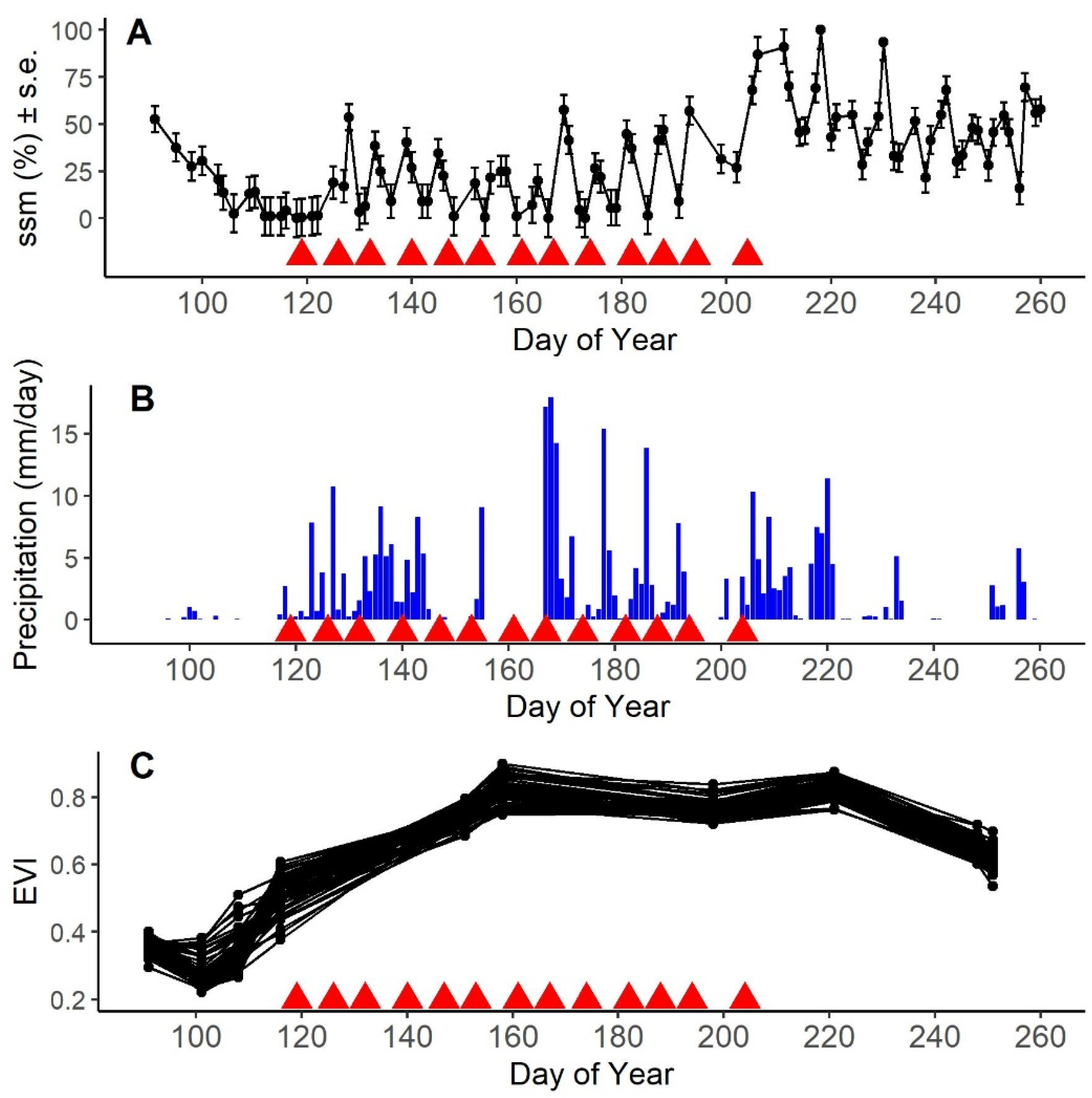
The start of the sampling season (DoY 119) was preceded by very low rainfall in the region and low surface soil moisture (Figure 2A,B). Later in the season, the peaks and troughs in surface soil moisture were driven by precipitation events throughout the sampling period and there was evidence of the repeated wetting and drying of the soil. A likely consequence of the very dry conditions in the spring was the slowing of the green-up. The first five sampling dates (DoY 119, 126, 132, 140 and 147) appeared to be during the green-up period of the grassland prior to the period of peak biomass (Figure 2C). Unfortunately, due to frequent cloud cover during 2021, the Sentinel-2 time series was sparse; so, the end of the green-up period was speculative but appeared to occur around DoY 160. The remaining eight sampling events took place during peak biomass.

3.2. Spectral Distance over Time

The lowest cumulative Euclidean distance and SAM value between pairs of spectra across all species occurred on day of year 174 (13 July 2021) and the highest occurred on day of year 204 (2 June 2021). There was a moderate to strong correlation between the pairwise spectral distances, whether calculated using SAM or the Euclidean distance (Spearman’s rank correlation = 0.7142857; p value = 0.008143).
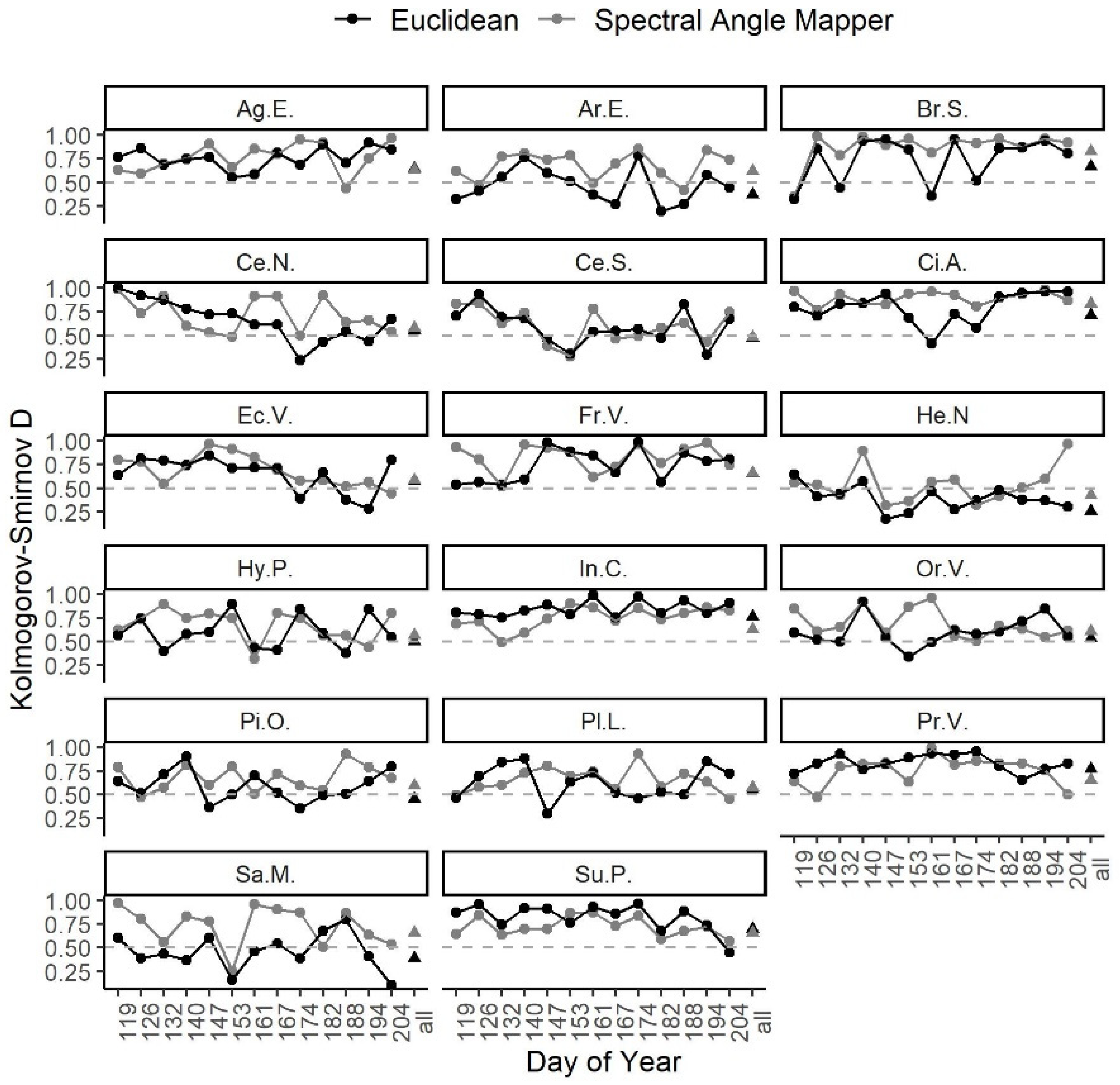
The mean intra-specific distances for each species and time point were smaller than the mean inter-specific distances for both distance metrics (bar Sanguisorba minor at DoY 153, 194 and 204). This indicated that the leaf samples that shared the same species were generally more spectrally similar (see Supplementary Materials Figures S2 and S3 for the distributions and means of the distances). The Kolmogorov–Smirnov test statistic (D) was used to determine whether the distribution of the intra-specific distances was significantly different from that of the inter-specific distances for each species at each time point. The values of D and their associated p values are presented in Figure 3. The values of D for five of the species (Primula vulgaris, Inula conyza, Fragaria vesca, Cirsium arvense and Agrimonia eupatoria) were always significant, regardless of the sampling point or distance metric. The values of D that were calculated using SAM were more stable in two of the species (Brachypodium sylvaticum and Cirsium arvense) than those that were calculated using the Euclidean distance. However, overall, there appeared to be no advantage to using either metric in terms of species separability from the single sampling point perspective. In contrast, the value of D was equivalent or larger for SAM than the Euclidean distance across all sampling dates for all species except Primula vulgaris and Inula conyza. So, cross-seasonally, SAM may be a more useful metric to use for species discrimination problems.

3.3. Performance of PLS-DA over Time: Waveband and Model Stability

The sPLS-DA models at each time point performed well, with overall model errors ranging from 0.02 on DoY 174 (23 June) to 0.12 on DoY 182 (1 July) (Table 1). The number of independent components that were required to obtain these low errors was quite high, ranging from 15 components on DoY 140 (20 May) to 21 components on several of the other dates. The number of wavebands that were used to obtain this level of classification ranged from 300 to 683, with 42–95% of available bands being exploited. In other words, even when using the sparse approach, a large proportion of the spectra was required to classify the 17 species for some time points and model runs.
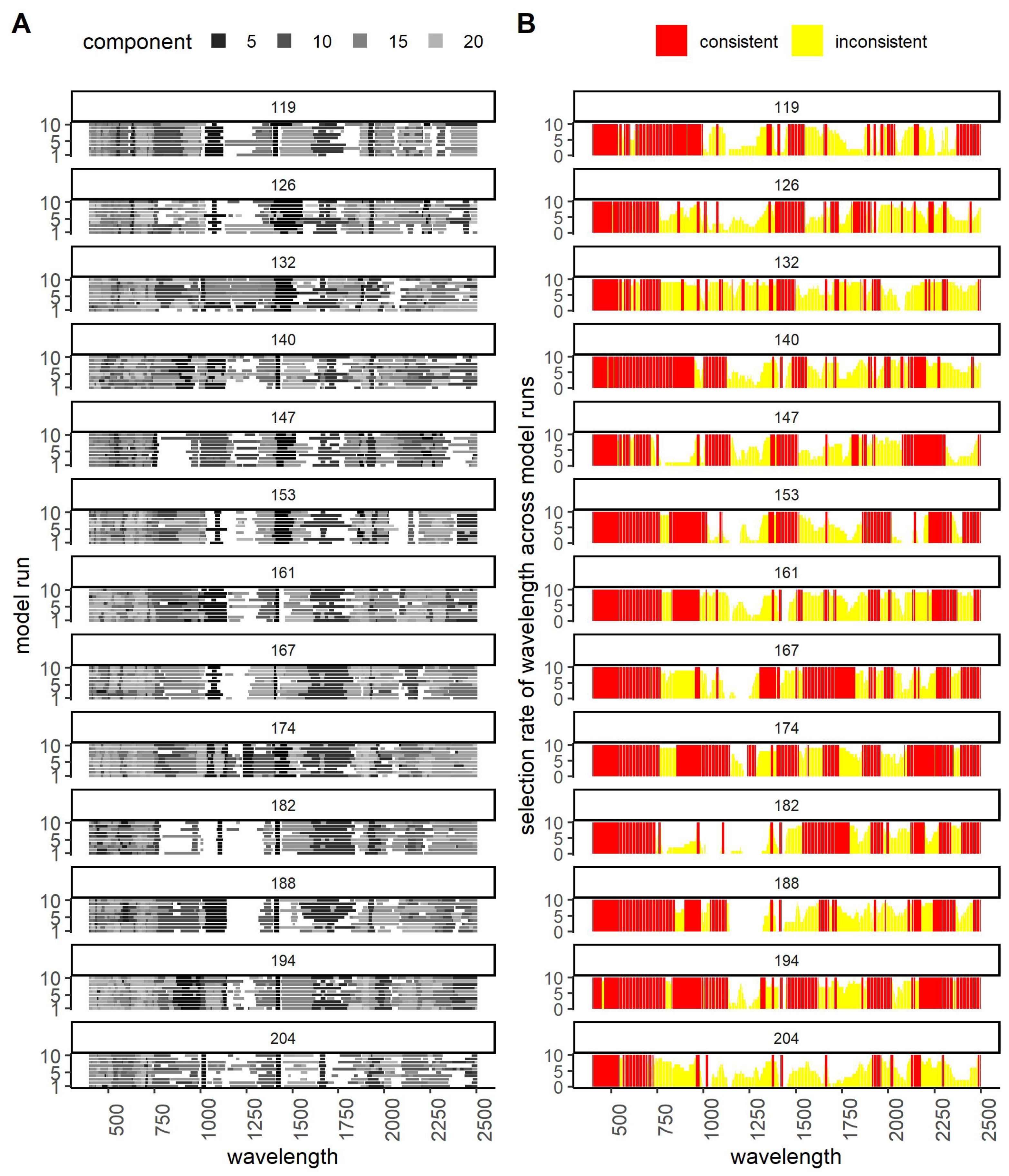
Within each time point, the variable selection across the 10 model runs was consistent for some wavebands but not for others (Figure 4). There were also multiple different solutions for the model at any one time in terms of waveband selection.
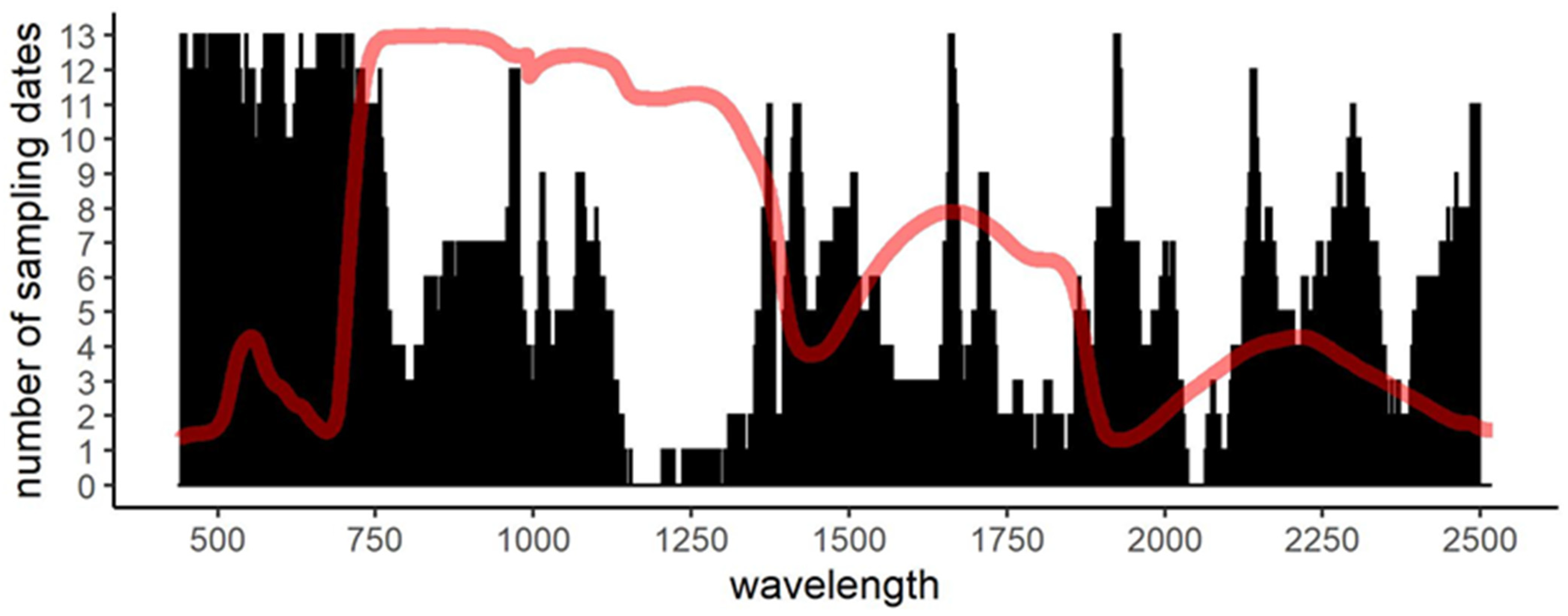
The wavebands that were consistently selected in all 10 models runs within a time point are shown in Figure 5. The number of times that these same wavebands were selected out of the 13 sampling dates is also shown. In total, 70 wavebands were selected in all model runs and time points (i.e., in 13 × 10 = 130 models) and 65 of these were in the visible part of the spectrum. The overlaid example spectrum in Figure 5 reveals the consistent general importance of wavelengths in both the visible and red-edge regions. Other important features can be seen at 1000 nm, the minimum points of reflectance in the SWIR at 1400 nm, 1950 nm and 2500 nm, the peak of 1800 nm in the SWIR and the slopes on either side of the peak at 2200 nm. The conformity of selection in the rough locations of important spectral features can also be observed. In contrast, there was a large variability in the exact location of band selection between sampling dates. Figure 4 and Figure 5 show the need to exploit much of the spectra to classify the taxonomic units.
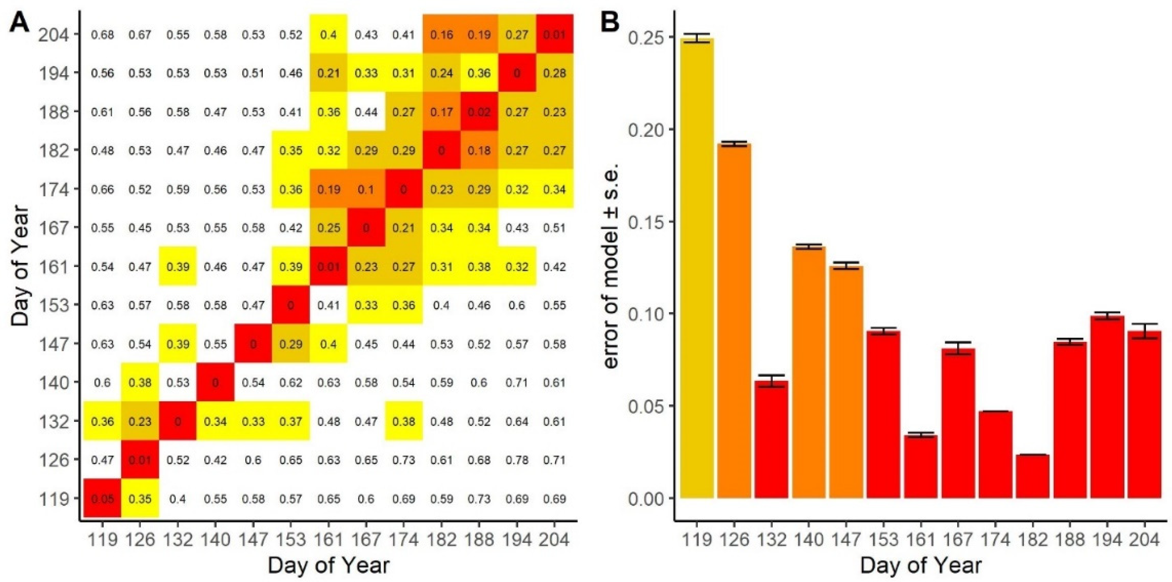
To assess model transferability across time, we tested the ability of the models that were trained using data from each sampling date to predict species using data from each of the other sampling dates (Figure 6A). We also used the model that was trained using all of the data to predict the species for each individual date (Figure 6B). In both cases, there was an observable increase in temporal dependence in the models after DoY 153. This stabilisation correlated with the end of “green-up” (see Figure 2C). When using the model that was trained using the cross-temporal data, the error rates were noticeably lower in the second half of the sampling campaign, which further indicated the stabilisation of waveband selection for species classification later in the growing season.

3.4. Ease of Species Separability

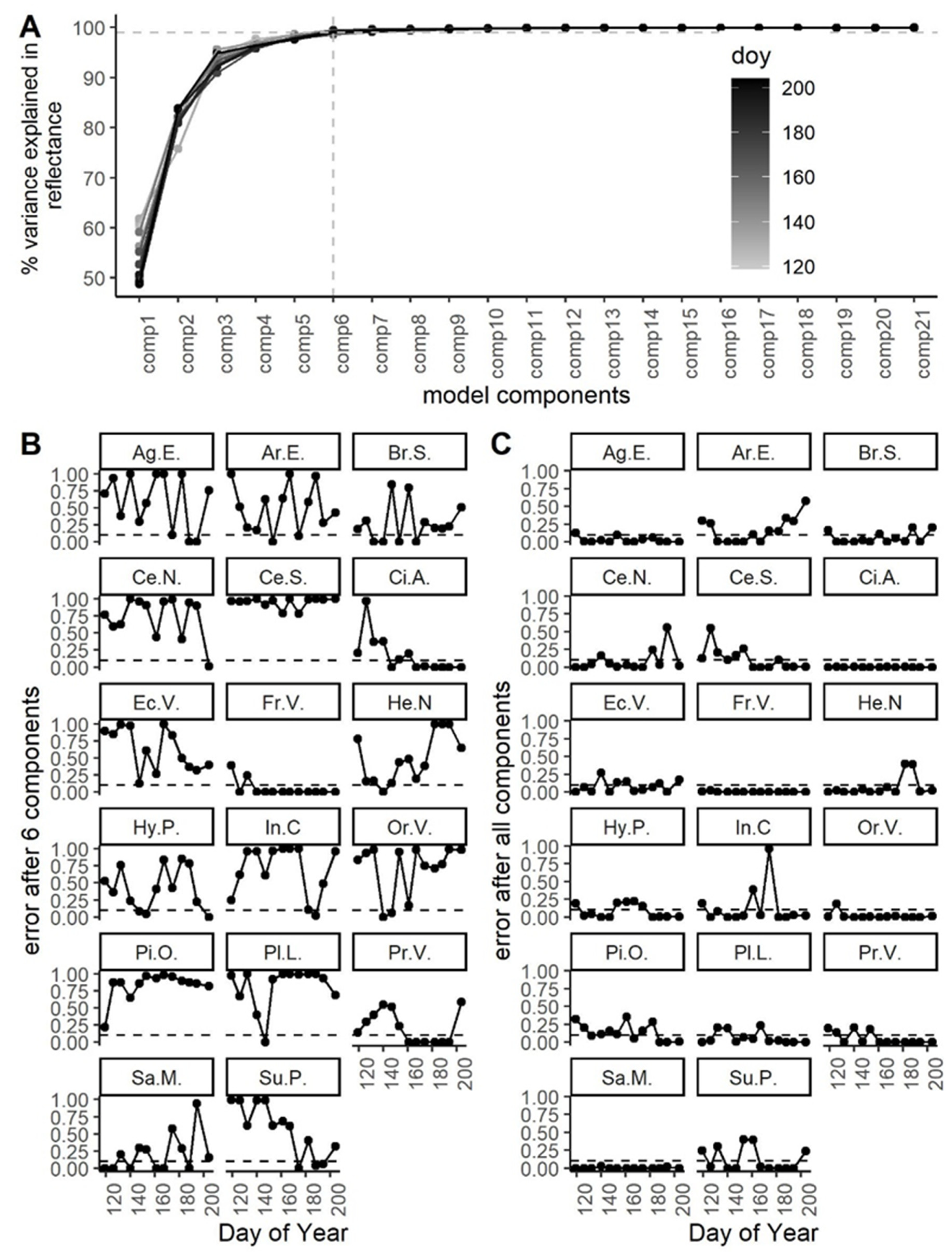
We noted that 99% of the spectral variance in the single date models was explained by only six independent components (see Figure 7A, the “scree plot” of the models). This was the case in all model runs and at all time points. The species classification error was examined for each species across time. With the recommended number of components in the model, all species achieved a satisfactory error rate (<0.1) for at least seven of the sampling dates. Three of the species (Cirsium acaule, Fragaria vesca and Sanguisorba minor) were well classified at all time points (Figure 7C). A very high error rate was found for Inula conyza on DoY 174. This was due to the low number of samples (n = 2) that was obtained for this species on this date. The class-based error rate of the 99% spectral variance and the six components was very stable across model runs within time points but overall, it was very temporally dependent (Figure 7B). Using this reduced number of components, almost all species (apart from Centaurea scabiosa) were well classified at certain times, but none of the species were consistently well classified, irrespective of the time point. The classification error was high for most species, which suggested that very small differences in spectral reflectance were responsible for most of the class differentiation of species within this community throughout the season.
We used the number of components that were required to achieve a classification error of less than 0.1 as an indicator of the “ease of classification” for each species. The mean value of the standard errors across all time points and models runs (n = 130) per species is presented in Figure 8A. Fragraia vesca and Cirsium acaule were clearly the easiest to classify according to our criteria. The other species all showed large standard errors around the mean, which implied that the ease of classification was more temporally dependent. The same evaluation was carried out for the sPLS-DA model that was trained using the cross-seasonal data (Figure 8B). These results provided a clearer picture, with six species requiring under 10 components to be well-classified, five species requiring between 10 and 20 components and the remaining six species being impossible to classify to the desired level of error. When the species were ranked from the easiest to hardest to classify, the means of the results from the single time points and the model that was trained using the cross-seasonal data were well correlated (Spearman’s rank correlation = 0.8). In the further analyses, the classification “ease” metric from each of the single time point models was used.

3.5. Phylogenetic and Morphological Drivers of Species Separability

We used linear models to test whether the ease of classification was related to the phylogenetic and morphological aspects of the community (see Figure 1C–E). Firstly, we tested whether smaller phylogenetic distances between pairs of species made them more difficult to separate. We found that phylogenetic distance was very weakly correlated with the ease of classification within this community (r2 = 0.05, slope = 0.03, p = 0.00287), with species that had smaller evolutionary distances being slightly harder to classify. We proposed that species with smaller leaves would be harder to measure using the leaf clip and that the measurements of these leaves would be subject to increased noise. However, we found no effects of leaf size on the ease of classification. We found bi-directional leaf reflectance at 445 nm to be very weakly correlated with the ease of separation; however, this finding was driven by two species (Helianthenum nummularium r2 = 0.36, slope = −119, p < 0.001 and Sanguisorba minor r2 = 0.168, slope = −98, p < 0.001). The more specular the reflectance, the easier these two species were to classify. We performed an ANOVA and a paired Tukey test to test whether leaf longevity or leaf surface mechanisms had any effects on classification ease. We found that aestival (spring emerging) leaves were harder to classify than evergreen and semi-evergreen leaves (ANOVA: F = 4.445, p < 0.05); the post hoc Tukey test showed that aestival leaves differed significantly from the other two groups at p = 0.03 and p = 0.01. We also found that species with spines were easier to classify than those with glabrous or hairy leaves (ANOVA: F = 8.552, p < 0.0001); post hoc Tukey test showed that spines differed significantly from the other two groups at p < 0.0001 and p < 0.001. However, this latter result should be treated with caution as only one species in the community had spines (Cirsium acaule).
By using the GSA of PRO-COSINE and the waveband selections from the sPLS-DA models, we were able to understand which leaf traits were likely to be the principal drivers of spectral variations within the plant community (Figure 9A). The consistent results for Component 1 (Figure 9B) highlighted the importance of the SWIR water feature in explaining the variances between species. Regardless of the sampling date, the wavebands that accounted for the largest amount of independent variation (between 49–61%) were situated in the region of Cw maximum, around 1410 nm. The second most variable region (21–35%) was represented by wavelength selections in the NIR at all time points, except for one (DoY 132). This is the region where the structural parameter of the leaf, N, is most strongly expressed. Component 3 represented variations in the visible region and hence, the region of chlorophyll expression. In the second half of the sampling season (DoY 161, 174, 182, 188 and 204), specular reflectance (bspec) also became an important trait for certain sampling dates. Components 4–6 captured variations in Cm that only represented between 1 and 5% of the total spectral variance.

4. Discussion

Using the sparse PLS-DA approach with leaf clip data, species were classifiable to a very good error rate of 0.1% in most cases across the season. This result was obtained using a small sample size (n = 5) per species per time point and it was possible to collect these samples for 17 species within a single sampling day. However, the models that were produced were complex and required between 15 and 21 components, depending on the sampling date and model run. These results suggest that species classification within complex communities will not be an easy task. In addition, 99% of the spectral variance for any one of the sampling dates was explained by only six model components. All model runs and sampling dates were very consistent in this respect. After the application of six components, most species displayed an unsatisfactory error rate for any single sampling date. This meant that a large amount of the discriminatory ability of reflectance data for the species was based on extremely small differences between spectra, which probably resulted from the complex co-varying relationships between the leaf optical traits.
The results from across the growing season showed that some species were consistently easy to classify using a small number of components. Another group was possible to identify but required more components, most of which represented a very small amount of the total spectral variance. The final group of species was impossible to classify to the desired error rate of 10% across time, but at certain time points, the species were well classified. For sampling campaigns in which data are collected during a single day, there is the possibility that species discrimination results from sampling errors and instrumental noise when it is based on very small differences in leaf spectra. It has been shown through simulation studies that when there are more than twice as many classes as samples, the PLS-DA readily finds a hyperplane that is stochastic in nature [43]. We showed that for species that are easy to classify, the model that was produced from cross-seasonal sampling merely confirmed the results of the models that were produced from single time points; however, for species that are more difficult to classify, it could provide confidence when discriminating between noise and biological signals.. We may be able to understand the reasons for the variations in classification error over time in some cases. For example, we saw that for two of the species examined here (Helianthenum nummularium and Sanguisorba minor), variations in specular reflectance over the course of a growing season strongly affected the ease of classification.
The result that 99% of the spectral variance classified only six species to less than a 10% error rate across time suggested that the ability of the SVH to hold at the leaf-level in single date sampling campaigns depended on the extent to which the community was composed of species that were “easy” to detect. SVH, as an unsupervised form of biodiversity assessment, assumes that cross-spectral variance in reflectance can account for the diversity of taxonomic units. However, from the results that are presented here, we could not infer that spectral variance was necessarily correlated with species numbers or their abundances.
The global variance decomposition that resulted from the radiative transfer modelling, alongside the waveband selections that were required for each model run, revealed that leaf EWT was the most important and consistent driver of spectral variance that was related to species classification, followed by N, Cab, bspec and LMA (although the relative importance of these traits was more temporally dependent). The importance of the wavebands that related to EWT did not vary with sampling date nor seasonal soil moisture content, as simulated by Sentinel-1. Grime’s CSR strategy and Ellenberg’s indicator values for the species that were examined here revealed a plant community that was dominated by stress tolerators and adapted to high pH soils. However, the moisture and nitrogen demand of these species was more variable. Similar sampling campaigns that involve the collection of leaf-level water content alongside leaf-level reflectance may help us to better understand why this feature is so important and whether this is limited to this type of stress tolerator system. The transferability of the models during the sampling period (day of year 161 to 204) could also coincide with the trait stabilisation of the leaves and, in turn, the stabilisation of the spectral representation of traits (waveband selection). Yang et al. [13] found that in tree leaves, LMA and chlorophyll a/b content increase with green-up and then remain steady until leaf fall.
The detection of leaf traits using reflectance data is optimal when using a leaf clip and integrating sphere [58], which provides both reflectance and transmittance. In contrast, bi-directional reflectance data that are obtained using a leaf clip result in the over-estimation of cross-spectral reflectance due to surface reflectance of the leaves. The application of the results of this study (and others that take a similar approach) in close range imaging spectroscopy requires a consideration of additional sources of variation that relate to anisotropy (light incident angle and illumination zenith angle). These variables can also be modelled using the COSINE radiative transfer model [54] but would be additional sources of uncertainty in species determination. Reflectance variance in grasslands at the very high-resolution canopy scale has already been attributed to non-taxonomic properties, such as the vertical complexity of the sward [59], the presence of mature leaves [25] and pixels containing soil [60]. In this work, we avoided sampling plants that were growing in shaded environments, but there is also evidence that chlorophyll levels vary between leaves that are in the sun and those that are in the shade [61]. These additional sources of variation are likely to further increase the difficulty of species discrimination using close range imaging spectroscopy.
Feature selection and classification model specifications over time could also be affected by methodological choices in the analysis. Here, we applied the sPLS-DA approach to data that were pre-processed using a Savitzky–Golay filter. When utilising close range imaging spectroscopy, spectra are likely to contain more noise than when using a leaf clip. Therefore, the type and optimal amount of spectral smoothing need to be examined in more detail and within differing instrumental contexts. Here, spectra were resampled to a 3-nm bandwidth; however, when optimising classification, the bandwidth choice within differing spectral regions could vary. Finally, sPLS-DA is only one modelling approach for classification and feature selection. In order to develop more robust species discrimination models over time, it is likely that more advanced methods would also need to be tested and compared [62,63].

5. Conclusions

To date, species discrimination tasks using hyperspectral data have generally been focused on woody species. Despite their conservation status and importance, herbaceous species are less studied and when they are, observations are mostly confined to the dominant species rather than attempting to capture the full botanical composition of the sward. Plant trait studies have shown that the spectral determination of the leaf properties of herbaceous species may be more difficult to obtain than that of the leaf properties of woody species [64]; therefore, we should practice caution when applying results from studies that are performed in forests to grasslands and we should instead conduct similar workon grassland communities.
In this study, we found that some species within a community framework were easier to discriminate across the season than others. This pointed to a relative distinction in their leaf reflectance properties. Other species that were more difficult to discriminate required complex waveband combinations, which fluctuated across time. Cross-seasonal sampling, even with small sample sizes, could help to verify which species are driving measures of spectral diversity. Studies that explore species-specific chemical and structural leaf properties and relate these to leaf spectral signatures [65] are needed to help us to explain with more certainty why some species are easier to distinguish than others and to create a predictive framework for species monitoring and diversity assessment using leaf reflectance. We recommend further studies that explore functional trait frameworks when making predictions of species classes and exploit GSMs and RTMs, alongside biochemical assays, to estimate the importance of traits across different scales and instruments.

Supplementary Materials

The following are available online at https://www.mdpi.com/article/10.3390/rs14102310/s1, Figure S1: Spectra at each pre-processing stage prior to inclusion in the sPLS-DA models, Figure S2: Differences in distributions using Euclidean Distance, Figure S3: Differences in distributions using SAM, Figure S4: Ease of classification based on the number of components.

Author Contributions

Conceptualisation, R.H.T., A.V., K.W. and F.F.G.; methodology, R.H.T.; software, R.H.T.; validation, K.W., A.V. and F.F.G., formal analysis, R.H.T.; investigation, R.H.T.; resources, R.H.T.; data curation, R.H.T.; writing—original draft preparation, R.H.T.; writing—review and editing, A.V., K.W. and F.F.G.; visualisation, R.H.T.; supervision, A.V.; project administration, R.H.T.; funding acquisition, A.V. and R.H.T. All authors have read and agreed to the published version of the manuscript.

Funding

The PhD studentship under which this research was carried out was funded by the NERC (Natural Environment Research Council), studentship grant NE/L002566/1. Field work expenses were funded by the Old Chalk New Downs Project.

Data Availability Statement

The data presented in this study are openly available through the NERC’s Centre for Environmental Data Analysis at http://dx.doi.org/10.5285/8a798466b9f74b3da500004a94ee5fee (accessed on 18 March 2022).

Conflicts of Interest

The authors declare no conflict of interest. The funders had no role in the design of the study, the collection, analyses or interpretation of data, the writing of the manuscript or the decision to publish the results.

References

  1. Critchley, C.N.R.; Burke, M.J.W.; Stevens, D.P. Conservation of lowland semi-natural grasslands in the UK: A review of botanical monitoring results from agri-environment schemes. Biol. Conserv. 2004, 115, 263–278. [Google Scholar] [CrossRef]
  2. de Bello, F.; Lavorel, S.; Gerhold, P.; Reier, Ü.; Pärtel, M. A biodiversity monitoring framework for practical conservation of grasslands and shrublands. Biol. Conserv. 2010, 143, 9–17. [Google Scholar] [CrossRef]
  3. Lark, T.J. Protecting our prairies: Research and policy actions for conserving America’s grasslands. Land Use Policy 2020, 97, 104727. [Google Scholar] [CrossRef]
  4. Mansour, K.; Mutanga, O.; Everson, T.; Adam, E. Discriminating indicator grass species for rangeland degradation assessment using hyperspectral data resampled to AISA Eagle resolution. ISPRS J. Photogramm. Remote Sens. 2012, 70, 56–65. [Google Scholar] [CrossRef]
  5. Marcinkowska-Ochtyra, A.; Jarocińska, A.; Bzdȩga, K.; Tokarska-Guzik, B. Classification of expansive grassland species in different growth stages based on hyperspectral and LiDAR data. Remote Sens. 2018, 10, 2019. [Google Scholar] [CrossRef] [Green Version]
  6. Pfitzner, K.; Bartolo, R.; Whiteside, T.; Loewensteiner, D.; Esparon, A. Hyperspectral monitoring of non-native tropical grasses over phenological seasons. Remote Sens. 2021, 13, 738. [Google Scholar] [CrossRef]
  7. Meireles, J.E.; Cavender-Bares, J.; Townsend, P.A.; Ustin, S.; Gamon, J.A.; Schweiger, A.K.; Schaepman, M.E.; Asner, G.P.; Martin, R.E.; Singh, A.; et al. Leaf reflectance spectra capture the evolutionary history of seed plants. New Phytol. 2020, 228, 485–493. [Google Scholar] [CrossRef]
  8. Irisarri, J.G.N.; Oesterheld, M.; Verón, S.R.; Paruelo, J.M. Grass species differentiation through canopy hyperspectral reflectance. Int. J. Remote Sens. 2009, 30, 5959–5975. [Google Scholar] [CrossRef]
  9. Punalekar, S.; Verhoef, A.; Tatarenko, I.V.; Van Der Tol, C.; Macdonald, D.M.J.; Marchant, B.; Gerard, F.; White, K.; Gowing, D. Characterization of a highly biodiverse floodplain meadow using hyperspectral remote sensing within a plant functional trait framework. Remote Sens. 2016, 8, 112. [Google Scholar] [CrossRef] [Green Version]
  10. Petibon, F.; Czyż, E.A.; Ghielmetti, G.; Hueni, A.; Kneubühler, M.; Schaepman, M.E.; Schuman, M.C. Uncertainties in measurements of leaf optical properties are small compared to the biological variation within and between individuals of European beech. Remote Sens. Environ. 2021, 264, 112601. [Google Scholar] [CrossRef]
  11. Wang, R.; Gamon, J.A.; Schweiger, A.K.; Cavender-Bares, J.; Townsend, P.A.; Zygielbaum, A.I.; Kothari, S. Influence of species richness, evenness, and composition on optical diversity: A simulation study. Remote Sens. Environ. 2018, 211, 218–228. [Google Scholar] [CrossRef]
  12. Price, J.C. How unique are spectral signatures? Remote Sens. Environ. 1994, 49, 181–186. [Google Scholar] [CrossRef]
  13. Yang, X.; Tang, J.; Mustard, J.F.; Wu, J.; Zhao, K.; Serbin, S.; Lee, J.E.; Noda, H.M.; Muraoka, H.; Nasahara, K.N. Seasonal variability of multiple leaf traits captured by leaf spectroscopy at two temperate deciduous forests. Agric. For. Meteorol. 2016, 179, 108236. [Google Scholar] [CrossRef] [Green Version]
  14. Chavana-Bryant, C.; Malhi, Y.; Wu, J.; Asner, G.P.; Anastasiou, A.; Enquist, B.J.; Cosio Caravasi, E.G.; Doughty, C.E.; Saleska, S.R.; Martin, R.E.; et al. Leaf aging of Amazonian canopy trees as revealed by spectral and physiochemical measurements. New Phytol. 2017, 214, 1049–1063. [Google Scholar] [CrossRef] [Green Version]
  15. Guo, C.; Ma, L.; Yuan, S.; Wang, R. Morphological, physiological and anatomical traits of plant functional types in temperate grasslands along a large-scale aridity gradient in northeastern China. Sci. Rep. 2017, 7, 40900. [Google Scholar] [CrossRef] [PubMed] [Green Version]
  16. Serbin, S.P.; Singh, A.; McNeil, B.E.; Kingdon, C.C.; Townsend, P.A. Spectroscopic determination of leaf morphological and biochemical traits for northern temperate and boreal tree species. Ecol. Appl. 2014, 24, 1651–1669. [Google Scholar] [CrossRef] [Green Version]
  17. Asner, G.P.; Martin, R.E. Canopy phylogenetic, chemical and spectral assembly in a lowland Amazonian forest. New Phytol. 2011, 189, 999–1012. [Google Scholar] [CrossRef]
  18. Hesketh, M.; Sánchez-Azofeifa, G.A. The effect of seasonal spectral variation on species classification in the Panamanian tropical forest. Remote Sens. Environ. 2012, 118, 73–82. [Google Scholar] [CrossRef]
  19. Dudley, K.L.; Dennison, P.E.; Roth, K.L.; Roberts, D.A.; Coates, A.R. A multi-temporal spectral library approach for mapping vegetation species across spatial and temporal phenological gradients. Remote Sens. Environ. 2015, 167, 121–134. [Google Scholar] [CrossRef]
  20. Wang, R.; Gamon, J.A.; Cavender-Bares, J.; Townsend, P.A.; Zygielbaum, A.I. The spatial sensitivity of the spectral diversity-biodiversity relationship: An experimental test in a prairie grassland. Ecol. Appl. 2018, 28, 541–556. [Google Scholar] [CrossRef] [Green Version]
  21. Schweiger, A.K.; Cavender-Bares, J.; Townsend, P.A.; Hobbie, S.E.; Madritch, M.D.; Wang, R.; Tilman, D.; Gamon, J.A. Plant spectral diversity integrates functional and phylogenetic components of biodiversity and predicts ecosystem function. Nat. Ecol. Evol. 2018, 2, 976–982. [Google Scholar] [CrossRef] [PubMed]
  22. Carlson, K.M.; Asner, G.P.; Hughes, R.F.; Ostertag, R.; Martin, R.E. Hyperspectral remote sensing of canopy biodiversity in Hawaiian lowland rainforests. Ecosystems 2007, 10, 536–549. [Google Scholar] [CrossRef]
  23. Féret, J.B.; Asner, G.P. Spectroscopic classification of tropical forest species using radiative transfer modeling. Remote Sens. Environ. 2011, 115, 2415–2422. [Google Scholar] [CrossRef]
  24. Gholizadeh, H.; Gamon, J.A.; Helzer, C.J.; Cavender-Bares, J. Multi-temporal assessment of grassland α- and β-diversity using hyperspectral imaging. Ecol. Appl. 2020, 30, e02145. [Google Scholar] [CrossRef] [PubMed]
  25. Thornley, R.; Gerard, F.F.; White, K.; Verhoef, A. Intra-annual taxonomic and phenological drivers of spectral variance in grasslands. Remote Sens. Environ. 2022, 271, 112908. [Google Scholar] [CrossRef]
  26. Imran, H.A.; Gianelle, D.; Scotton, M.; Rocchini, D.; Dalponte, M.; Macolino, S.; Sakowska, K.; Pornaro, C.; Vescovo, L. Potential and limitations of grasslands α-diversity prediction using fine-scale hyperspectral imagery. Remote Sens. 2021, 13, 2649. [Google Scholar] [CrossRef]
  27. Maschler, J.; Atzberger, C.; Immitzer, M. Individual tree crown segmentation and classification of 13 tree species using Airborne hyperspectral data. Remote Sens. 2018, 10, 1218. [Google Scholar] [CrossRef] [Green Version]
  28. Dalponte, M.; Ørka, H.O.; Ene, L.T.; Gobakken, T.; Næsset, E. Tree crown delineation and tree species classification in boreal forests using hyperspectral and ALS data. Remote Sens. Environ. 2014, 140, 306–317. [Google Scholar] [CrossRef]
  29. Lopatin, J.; Fassnacht, F.E.; Kattenborn, T.; Schmidtlein, S. Mapping plant species in mixed grassland communities using close range imaging spectroscopy. Remote Sens. Environ. 2017, 201, 12–23. [Google Scholar] [CrossRef]
  30. Peerbhay, K.Y.; Mutanga, O.; Ismail, R. Commercial tree species discrimination using airborne AISA Eagle hyperspectral imagery and partial least squares discriminant analysis (PLS-DA) in KwaZulu-Natal, South Africa. ISPRS J. Photogramm. Remote Sens. 2013, 79, 19–28. [Google Scholar] [CrossRef]
  31. Zhong, Y.; Hu, X.; Luo, C.; Wang, X.; Zhao, J.; Zhang, L. WHU-Hi: UAV-borne hyperspectral with high spatial resolution (H2) benchmark datasets and classifier for precise crop identification based on deep convolutional neural network with CRF. Remote Sens. Environ. 2020, 250, 112012. [Google Scholar] [CrossRef]
  32. Vaiphasa, C.; Skidmore, A.K.; de Boer, W.F.; Vaiphasa, T. A hyperspectral band selector for plant species discrimination. ISPRS J. Photogramm. Remote Sens. 2007, 62, 225–235. [Google Scholar] [CrossRef]
  33. Fassnacht, F.E.; Latifi, H.; Stereńczak, K.; Modzelewska, A.; Lefsky, M.; Waser, L.T.; Straub, C.; Ghosh, A. Review of studies on tree species classification from remotely sensed data. Remote Sens. Environ. 2016, 186, 64–87. [Google Scholar] [CrossRef]
  34. Hennessy, A.; Clarke, K.; Lewis, M. Hyperspectral Classification of Plants: A Review of Waveband Selection Generalisability. Remote Sens. 2020, 12, 113. [Google Scholar] [CrossRef] [Green Version]
  35. Fitter, A.H.; Peat, H.J. The Ecological Flora Database. J. Ecol. 1994, 82, 415–425. Available online: http://www.ecoflora.co.uk (accessed on 2 February 2022). [CrossRef]
  36. Grime, J.P. Trait convergence and trait divergence in herbaceous plant communities: Mechanisms and consequences. J. Veg. Sci. 2006, 17, 255. [Google Scholar] [CrossRef]
  37. Grime, J.P.; Hodgeson, J.G.; Hunt, R. The Autecological Accounts. In Comparative Plant Ecology; Oxford University Press: Oxford, UK, 1998; pp. 53–646. [Google Scholar]
  38. Alexander, L.V.; Jones, P.D. Updated precipitation series for the U.K. and discussion of recent extremes. Atmos. Sci. Lett. 2001, 1, 142–150. [Google Scholar] [CrossRef]
  39. Schweiger, A.K. Spectral field campaigns: Planning and data collection. In Remote Sensing of Plant Biodiversity; Cavender-Bares, J., Gamon, J.A., Townsend, P.A., Eds.; Springer Nature: Cham, Switzerland, 2020; pp. 385–423. [Google Scholar]
  40. Lehnert, L.W.; Meyer, H.; Obermeier, W.A.; Silva, B.; Regeling, B.; Thies, B.; Bendix, J. Hyperspectral data analysis in R: The hsdar package. J. Stat. Softw. 2019, 89, 1–23. [Google Scholar] [CrossRef] [Green Version]
  41. Kruse, F.A.; Lefkoff, A.B.; Boardman, J.W.; Heidebrecht, K.B.; Shapiro, A.T.; Barloo, P.J.; Goetz, A.F.H. The Spectral Image Processing System (SIPS)- Interactive Visualization and Analysis of Imaging Spectrometer Data. Remote Sens. Environ. 1993, 44, 145–163. [Google Scholar] [CrossRef]
  42. Marsaglia, G.; Tsang, W.W.; Wang, J. Evaluating Kolmogorov’s distribution. J. Stat. Softw. 2003, 8, 1–4. [Google Scholar] [CrossRef]
  43. Ruiz-Perez, D.; Guan, H.; Madhivanan, P.; Mathee, K.; Narasimhan, G. So you think you can PLS-DA? BMC Bioinform. 2020, 21 (Suppl. 1), 1–10. [Google Scholar] [CrossRef] [PubMed]
  44. Mehmood, T.; Sæbø, S.; Liland, K.H. Comparison of variable selection methods in partial least squares regression. J. Chemom. 2020, 34, 1–14. [Google Scholar] [CrossRef] [Green Version]
  45. Feret, J.B.; François, C.; Asner, G.P.; Gitelson, A.A.; Martin, R.E.; Bidel, L.P.R.; Ustin, S.L.; le Maire, G.; Jacquemoud, S. PROSPECT-4 and 5: Advances in the leaf optical properties model separating photosynthetic pigments. Remote Sens. Environ. 2008, 112, 3030–3043. [Google Scholar] [CrossRef]
  46. Saccenti, E.; Timmerman, M.E. Approaches to sample size determination for multivariate data: Applications to PCA and PLS-DA of omics data. J. Proteome Res. 2016, 15, 2379–2393. [Google Scholar] [CrossRef]
  47. Lee, L.C.; Liong, C.Y.; Jemain, A.A. Partial least squares-discriminant analysis (PLS-DA) for classification of high-dimensional (HD) data: A review of contemporary practice strategies and knowledge gaps. Analyst 2018, 143, 3526–3539. [Google Scholar] [CrossRef]
  48. Rohart, F.; Gautier, B.; Singh, A.; Lê Cao, K.A. mixOmics: An R package for ‘omics feature selection and multiple data integration. BioRxiv 2017, 13, 1–19. [Google Scholar] [CrossRef] [Green Version]
  49. R Core Team, R. A Language and Environment for Statistical Computing; R Foundation for Statistical Computing: Vienna, Austria, 2021; Available online: https://www.R-project.org/ (accessed on 18 March 2022).
  50. Lê Cao, K.A.; Boitard, S.; Besse, P. Sparse PLS discriminant analysis: Biologically relevant feature selection and graphical displays for multiclass problems. BMC Bioinform. 2011, 12, 1–17. [Google Scholar] [CrossRef] [Green Version]
  51. Jin, Y.; Qian, H.V. PhyloMaker: An R package that can generate very large phylogenies for vascular plants. Ecography 2019, 42, 1353–1359. [Google Scholar] [CrossRef] [Green Version]
  52. Sims, D.A.; Gamon, J.A. Relationships between leaf pigment content and spectral reflectance across a wide range of species, leaf structures and developmental stages. Remote Sens. Environ. 2002, 81, 337–354. [Google Scholar] [CrossRef]
  53. Jacquemoud, S.; Baret, F. PROSPECT: A model of leaf optical properties spectra. Remote Sens. Environ. 1990, 34, 75–91. [Google Scholar] [CrossRef]
  54. Jay, S.; Bendoula, R.; Hadoux, X.; Féret, J.B.; Gorretta, N. A physically-based model for retrieving foliar biochemistry and leaf orientation using close-range imaging spectroscopy. Remote Sens. Environ. 2016, 177, 220–236. [Google Scholar] [CrossRef] [Green Version]
  55. Li, D.; Cheng, T.; Jia, M.; Zhou, K.; Lu, N.; Yao, X.; Tian, Y.; Zhu, Y.; Cao, W. PROCWT: Coupling PROSPECT with continuous wavelet transform to improve the retrieval of foliar chemistry from leaf bidirectional reflectance spectra. Remote Sens. Environ. 2018, 206, 1–14. [Google Scholar] [CrossRef]
  56. Wan, L.; Zhang, J.; Xu, Y.; Huang, Y.; Zhou, W.; Jiang, L.; He, Y.; Cen, H. PROSDM: Applicability of PROSPECT model coupled with spectral derivatives and similarity metrics to retrieve leaf biochemical traits from bidirectional reflectance. Remote Sens. Environ. 2021, 267, 112761. [Google Scholar] [CrossRef]
  57. Verrelst, J.; Rivera, J.P.; Moreno, J. ARTMO’s global sensitivity analysis (GSA) toolbox to quantify driving variables of leaf and canopy radiative transfer models. EARSeL eProceedings 2015, 2, 1–11. [Google Scholar]
  58. Hovi, A.; Forsström, P.; Mõttus, M.; Rautiainen, M. Evaluation of accuracy and practical applicability of methods for measuring leaf reflectance and transmittance spectra. Remote Sens. 2018, 10, 25. [Google Scholar] [CrossRef] [Green Version]
  59. Conti, L.; Malavasi, M.; Galland, T.; Komárek, J.; Lagner, O.; Carmona, C.P.; de Bello, F.; Rocchini, D.; Šímová, P. The relationship between species and spectral diversity in grassland communities is mediated by their vertical complexity. Appl. Veg. Sci. 2021, 24, 1–8. [Google Scholar] [CrossRef]
  60. Gholizadeh, H.; Gamon, J.A.; Zygielbaum, A.I.; Wang, R.; Schweiger, A.K.; Cavender-Bares, J. Remote sensing of biodiversity: Soil correction and data dimension reduction methods improve assessment of α-diversity (species richness) in prairie ecosystems. Remote Sens. Environ. 2018, 206, 240–253. [Google Scholar] [CrossRef]
  61. Murchie, E.H.; Horton, P. Acclimation of photosynthesis to irradiance and spectral quality in British plant species: Chlorophyll content, photosynthetic capacity and habitat preference. Plant Cell Environ. 1997, 20, 438–448. [Google Scholar] [CrossRef]
  62. Douzas, G.; Bacao, F.; Fonseca, J.; Khudinyan, M. Imbalanced learning in land cover classification: Improving minority classes’ prediction accuracy using the geometric SMOTE algorithm. Remote Sens. 2019, 11, 3040. [Google Scholar] [CrossRef] [Green Version]
  63. Banerjee, B.P.; Raval, S. A particle swarm optimization based approach to pre-tune programmable hyperspectral sensors. Remote Sens. 2021, 13, 3295. [Google Scholar] [CrossRef]
  64. Roelofsen, H.D.; van Bodegom, P.M.; Kooistra, L.; Witte, J.P.M. Predicting leaf traits of herbaceous species from their spectral characteristics. Ecol. Evol. 2014, 4, 706–719. [Google Scholar] [CrossRef] [PubMed]
  65. Falcioni, R.; Moriwaki, T.; Pattaro, M.; Herrig Furlanetto, R.; Nanni, M.R.; Camargos Antunes, W. High resolution leaf spectral signature as a tool for foliar pigment estimation displaying potential for species differentiation. J. Plant Physiol. 2020, 249, 153161. [Google Scholar] [CrossRef] [PubMed]
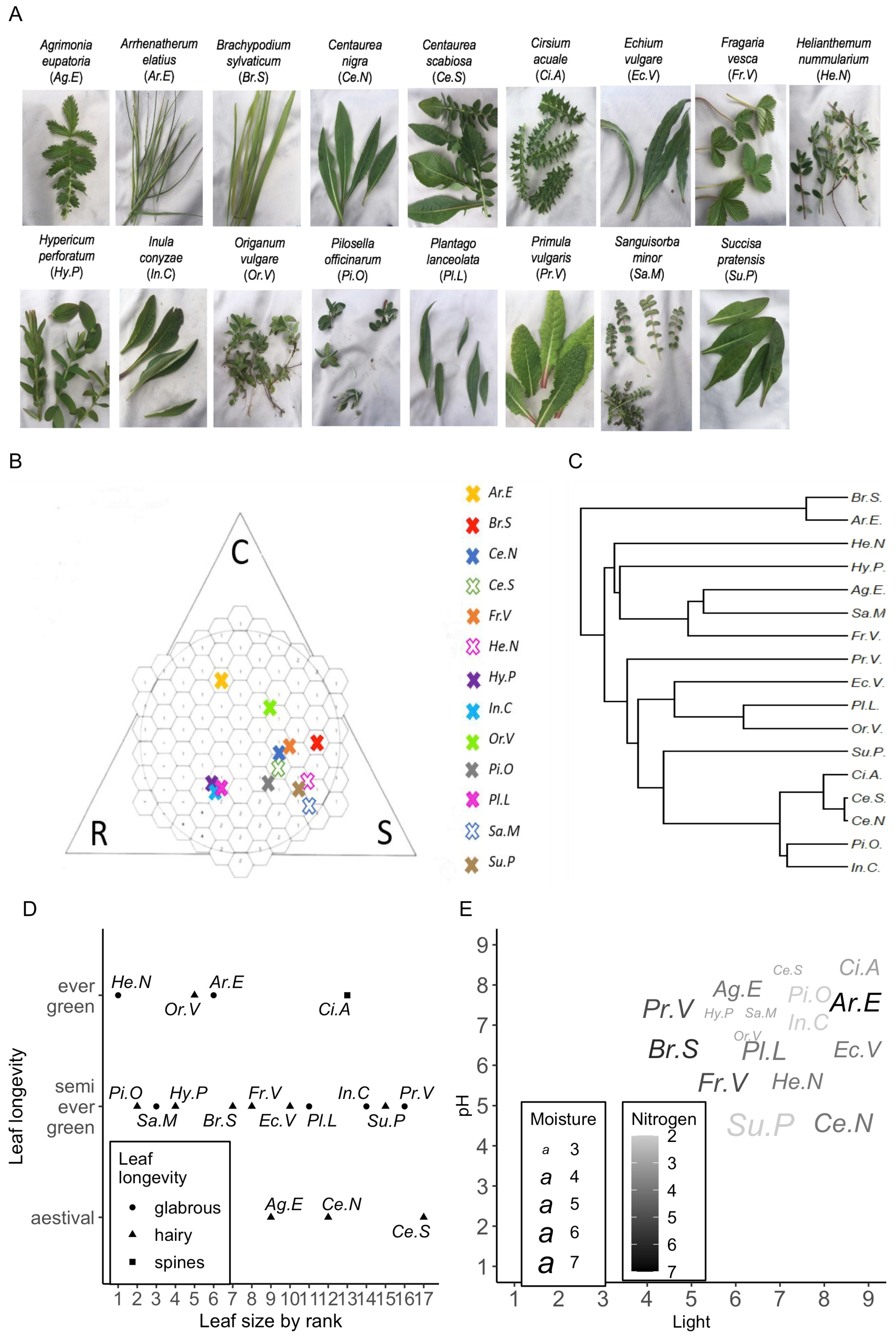
Figure 1. (A) The 17 grassland species that were involved in this study; (B) a plot of 13 of those species within the Grime strategy space, where data were available; (C) the phylogenetic relationship between species; (D) the morphological and phenological characteristics of the leaves; (E) Ellenberg’s indicator values for light, moisture, pH and nitrogen.
Remotesensing 14 02310 g001
Figure 2. (A) Satellite-derived time series of surface soil moisture (Sentinel-1) at a 1-km resolution; (B) regional daily precipitation averages; (C) the site-based green-up trajectory using EVI (Sentinel-2) at a 10-m resolution. The 13 field sampling dates are shown as red triangles.
Remotesensing 14 02310 g002
Figure 3. The value of D (the Kolmogorov–Smirnov statistic): a test of whether the distributions of the intra-specific and inter-specific distances were different from each other at each time point and across all sampling dates for each species class. The results are shown for both the Spectral Angle Mapper and the Euclidean distance. The values of D ranged from 1–0, with higher values representing distributions that were more distinct. A p value = 0.01 for the test is shown by a dashed line. Values above the line denote significantly different distributions.
Remotesensing 14 02310 g003
Figure 4. (A) The position within the spectra of components (latent variables) that were used for species–class determination for the 13 dates (day of year presented in the banner header). The darkest greys indicate components that captured more variations in the spectral data. (B) The selection rate of wavebands for model runs within each sampling date. Red bars represent wavelengths that were consistently selected in 10/10 runs; yellow bars are those that were only selected for some of the model runs.
Remotesensing 14 02310 g004
Figure 5. The number of times within each of the 13 sampling dates that wavebands were consistently selected in all model runs. A reference leaf spectrum (red line) is superimposed on the plot for contextualisation.
Remotesensing 14 02310 g005
Figure 6. (A) Confusion matrix of the mean errors of the 10 model runs that were trained using data from single sampling dates and tested using data that were collected on the other sampling dates. The temporal dependence of the data was higher after DoY 153. (B) The error of the model that was trained using data from all sampling dates and tested using data from single sampling dates. The error bars show the standard error of the mean model error after 10 runs.
Remotesensing 14 02310 g006
Figure 7. (A) The “scree plot” of the models at each time point, i.e., the variance in the X variable as explained by the model latent variables/components. The grey reference line represents the 99% variance in the X variable that was captured by six components, irrespective of sampling time; (B) species classification error over time with six components; (C) species classification error with the chosen number of components (i.e., the final model for each time point). Mean error is shown for each time point over the 10 model runs (the S.E. of the model runs was very small and is not shown).
Remotesensing 14 02310 g007
Figure 8. The “ease” of classification, defined as the number of components (latent variables) produced from the sPLS-DA models that were required to classify a species to a <10% error rate. Species are ranked from easiest to hardest to classify (left to right); (A) the mean and SE of the models across sampling dates; (B) the results from the model that was trained using the cross-seasonal dataset. Shaded bars show the species that were not classifiable to the required error rate.
Remotesensing 14 02310 g008
Figure 9. (A) The global sensitivity analysis of the radiative transfer model PRO-COSINE for leaf clip data with overlaid waveband selection for the first six components for two example time points (DoY 153 and 161); (B) the probability of the importance of traits for each of the six components over time using the wavelength selection from the best performing sPLS-DA models for each sampling date. The range of variance between model runs for each model component is presented in the panel header.
Remotesensing 14 02310 g009
Table 1. A summary of the results of the cumulative spectral distances and sPLS-DA models for each sampling date.
Sampling DateDateDay of Year (DoY)Cumulative
Distance
(Euclidean)
Cumulative
Distance
(Spectral Angle
Mapper)
Model Error (Range of 10 Runs; 2 d.p.)Number of Components (Range of 10 Runs)Number of Unique
Wavelengths (Range of 10 Runs)
129 April11912,398,26749700.1–0.1118–20467–576
26 May12612,504,25648740.09–0.120–21444–541
312 May13211,961,45748890.07–0.1118–20518–663
420 May14013,740,15550870.07–0.1115–21438–630
527 May14713,645,12650410.04–0.0416–17439–554
62 June15312,610,07149400.08–0.1120–21436–555
710 June16111,830,26547780.08–0.0819–20442–658
816 June16712,367,52048240.04–0.0818–20493–621
923 June17411,581,84346910.02–0.0520–21582–683
101 July18212,825,58950140.08–0.1216–19403–545
117 July18812,582,15951190.04–0.0819–20463–574
1213 July19412,329,16451040.05–0.0819–21583–641
1323 July20413,851,28551460.05–0.0719–20300–593
Publisher’s Note: MDPI stays neutral with regard to jurisdictional claims in published maps and institutional affiliations.