Class-Shared SparsePCA for Few-Shot Remote Sensing Scene Classification

Abstract

In recent years, few-shot remote sensing scene classification has attracted significant attention, aiming to obtain excellent performance under the condition of insufficient sample numbers. A few-shot remote sensing scene classification framework contains two phases: (i) the pre-training phase seeks to adopt base data to train a feature extractor, and (ii) the meta-testing phase uses the pre-training feature extractor to extract novel data features and design classifiers to complete classification tasks. Because of the difference in the data category, the pre-training feature extractor cannot adapt to the novel data category, named negative transfer problem. We propose a novel method for few-shot remote sensing scene classification based on shared class Sparse Principal Component Analysis (SparsePCA) to solve this problem. First, we propose, using self-supervised learning, to assist-train a feature extractor. We construct a self-supervised assisted classification task to improve the robustness of the feature extractor in the case of fewer training samples and make it more suitable for the downstream classification task. Then, we propose a novel classifier for the few-shot remote sensing scene classification named Class-Shared SparsePCA classifier (CSSPCA). The CSSPCA projects novel data features into subspace to make reconstructed features more discriminative and complete the classification task. We have conducted many experiments on remote sensing datasets, and the results show that the proposed method dramatically improves classification accuracy.

1. Introduction

The classification of aerial data and remote sensing data is significant in land use and cover [1,2,3], vegetation coverage [4], resource investigation [5], natural disaster observation [6,7], environmental monitoring [8] and ship monitoring [9,10]. Many deep learning methods based on big data have recently achieved excellent performance on classification tasks. However, these deep learning classification methods [9,10,11,12,13,14,15,16,17,18,19] need to rely on extensive data for training to achieve good results. In the case of limited data or expensive data acquisition, the application of models based on deep learning is limited, such as the field of remote sensing. Recently, more and more researchers have paid attention to the small sample learning method, which aims to learn classification tasks using a few samples. We propose a few-shot classification method for remote sensing scene classification in this work.

At present, the few-shot remote sensing scene classification method mainly includes two stages: the pre-training stage of the feature extractor and the meta-testing stage. In the pre-training stage, we use base data to train the feature extractor and obtain the feature extractor with the best performance. In the meta-testing stage, we use the pre-training feature extractor to extract the features of novel data. At each stage, there are two main challenges that are affected by the small amount of data.

The first challenge is that of how to train a perfect feature extractor. The main reason for this difficulty is that the feature extractor is affected by insufficient training data in the pre-trained stage. The model is easy to overfit or underfit in the training process. The poor performance of feature extractors prevents the extracted samples from having more discriminated features. Therefore, it is necessary to practice several measures to improve the performance of the feature extractor. Recently, there have been several attempts to solve this problem. The prototypical network [20] proposed by Snell, J. et al. used a four-layer neural network as the feature extractor. When there are fewer training data, the neural network has fewer layers and is not easily over-fitted. At the same time, the meta-learning method is adopted to train the feature extractor, which is different from the traditional training method that can judge all categories in the training dataset. This method subtracts N categories from the dataset as a meta-task, and N is usually 5. Using different meta-tasks to train the model continuously improves the model’s generalization performance and avoids under-fitting. However, this method is affected by the shallow depth of the neural network, which cannot extract deeper representation features of the image, limiting the classification performance of this method.

Unlike the prototypical network, Metaopt [21,22,23] used Resnet-12 with the twelve-layer neural network as the backbone. When using the deep convolutional network to extract features, the deeper network depth is, the better feature discrimination is. At the same time, a residual block is added to the network to solve the problem of model performance degradation with the deepening of the model. Metaopt achieved better performance, and then it gradually became the primary feature extractor for few-shot image classification.

Different from the training strategies adopted by the previous two methods, Tian, Y. et al. [24] found that finding a feature extractor with sufficient learning was more effective than the complex meta-learning algorithm. Instead of extracting the meta-task training model during training, they used the traditional classification training method. During the meta-testing stage, the steps are to remove the softmax layer of the neural network as the feature extractor and then use a simple linear classification to achieve excellent classification performance. In our proposed method, we use this simple and effective training method to train the feature extractor. Compared with the meta-learning training method, the model trained by this method is more robust and more suitable for transfer learning. At the same time, to further improve the performance of the feature extractor, we use the standard classification cross-entropy loss and attach self-supervised loss to enhance the performance of the feature extractor.

The second challenge is how to design a robust classifier using a limited number of samples (usually one or five) in the meta-testing phase. In remote sensing scene classification tasks, most previous works have tried to complete these through pre-trained models. Hu, F. et al. [13] employ transfer learning methods to apply pre-trained models in the ImageNet dataset on the remote sensing scene classification of high-resolution remote sensing imagery, which has achieved excellent performance. Cheng, G. et al. [15] used remote sensing datasets to fine-tune pre-trained networks to make pre-trained networks satisfy remote sensing classification tasks more adaptable. In the most novel research, Cheng, G. et al. [14] proposed the method that made use of lots of existing CNN models, exchanged a new discriminant objective function optimization model in the training stage and minimized the classification error while imposing a metric learning regularization, which reached the current optimal performance.

Nevertheless, these methods cannot be well applied to few-shot remote sensing scene classification. On the one hand, in the meta-testing stage, each category usually has only one or five training samples. The fine-tune method will lead to over-fitted and further decline of model performance. On the other hand, due to the excessive domain shift between the few-shot image classification dataset and the existing remote sensing dataset, the pre-trained model on the few-shot dataset cannot adapt to the remote sensing data well, referred to as a problem of “negative transfer”, which will seriously affect the classification performance. To solve this problem, we focus on improving the discrimination of novel data features and propose to use the Class-Shared Sparse PCA method to train and reconstruct features. Sparse PCA [25] (Sparse Principal Component Analysis) is widely used in data processing and dimensionality reduction, which is an extension of the standard PCA method [26] (Principal Component Analysis). In this paper, we extended Sparse PCA and named Class-Shared Sparse PCA. Figure 1 shows the distribution of the novel data features and the features reconstructed using our method. First, we map the novel data’s features into a more discriminative subspace and reconstruct features to obtain more discriminative features. Then, we adopt the reconstructed features to complete the classification task.

Figure 1. The framework of CSSPCA.

The main contributions of this paper are as follows.

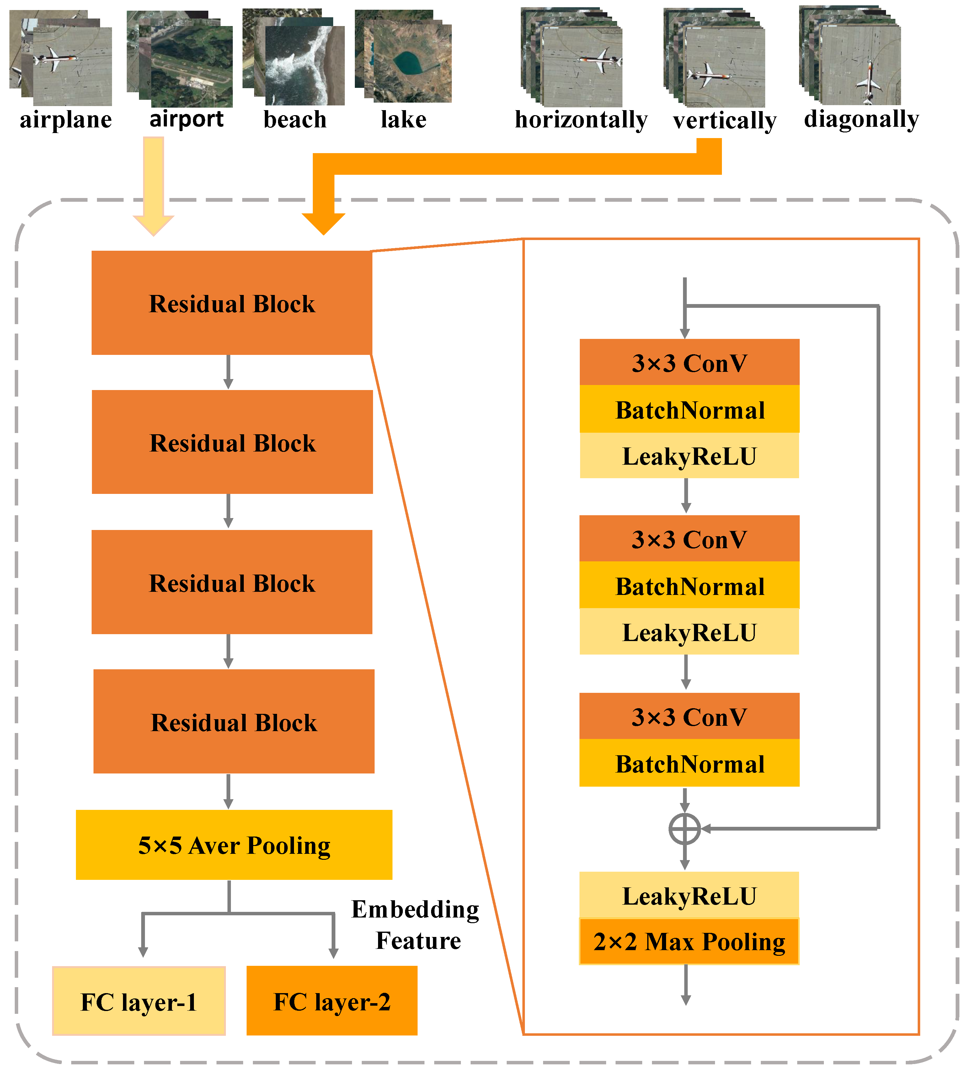
• We use self-supervised learning-assisted feature extractor training since the few-shot remote sensing scene data are thus less likely to over-fit the model problem. By constructing self-supervised auxiliary data and labels, the model performance is improved effectively.
• We introduce the subspace learning method into the framework of the few-shot remote sensing scene classification task and propose a novel method: the few-shot remote sensing scene classification method. Further experiments show that the proposed method can effectively solve the problem of “negative migration”.
• We propose a novel few-shot remote sensing scene classification based on the Class-Shared SparsePCA method, called CSSPCA. The CSSPCA maps the novel data features to more discriminant subspace to obtain more discriminant reconstruction features, thus improving classification performance.
• We test on two few-shot remote sensing scene datasets that have proved our proposed method’s validity and rationality.

2. Related Work

This section will review the related works about few-shot remote sensing scene classification and the problem of negative transfer in the pre-trained model.

Few-Shot Remote Sensing Scene Classification. Over the past few years, remote sensing scene classification has drawn the attention of researchers as a result of its widespread applications. As a spurt of progress in deep learning, these methods have gradually become the mainstream approaches. Still, deep learning places huge demands on labeled data, while there are inadequate data with expensive acquisition costs in the remote sensing field, which has restricted development in this area. In recent years, in order to solve the problem of limited data in some scenarios, researchers have proposed the method of few-shot learning and made remarkable progress. Therefore, few-shot learning further promotes the practical application of deep learning in the remote sensing field. At present, there are two main methods of few-shot learning based on remote sensing data: few-shot remote sensing scene classification based on optimization and based on metric learning.

Few-shot remote sensing scene classification based on optimization mainly utilizes the MAML [27] proposed by Finn, C. et al. and its improved methods [28,29]. By learning the model’s initialization parameters, the MAML maximized the precision on a new task after one step or several iterations and learned a feature that can be adapted to many tasks through optimization. This approach achieved better generalization performance with a few iterative steps. The model is easier to fine-tune while not requiring to care about the model’s form and adding new parameters. Meanwhile, it can perform gradient descent on new tasks quickly from previous tasks without an over-fitted problem. Dalal, A. A. et al. [30] applied the MAML algorithm to remote sensing scene classification tasks, achieving encouraging performance in the case of limited remote sensing data.

Few-shot remote sensing scene classification based on metric learning is a combination of metric learning and few-shot learning. Its basic principle is to independently learn the distance measurement function for a specific task according to different tasks. Many methods based on metric learning have been applied to few-shot remote sensing scene classification and have achieved excellent results in recent years.

The prototypical network [20] proposed by Snell, J. et al. was a simple and efficient method of few-shot learning. First, a few samples provided by each category are used to calculate the prototype of each class. The samples can realize the class by calculating the euclidean distance between their embedding features and these prototypes. Alajaji, D. et al. [31] applied the metric learning method of the prototypical network to remote sensing scene classification tasks. They used pre-trained SqueezeNet as a feature extractor, which is a simple and effective method. Zhang, P. et al. [32] also applied the prototypical network to remote sensing scene classification. They used remote sensing data to train feature extractors and finally measured the similarity between sample and prototype by cosine distance. The prototypical network is straightforward and powerful and has achieved outstanding performance in remote sensing scene classification tasks. However, due to the lack of training data, the prototype is prone to be affected by isolated samples, resulting in an inaccurate prototype and weak robustness.

Li, L. et al. [33] proposed a few-shot remote sensing scene classification method based on the matching network. The matching network [34] mapped images to an embedded space containing the label distribution, used different architectures to reflect the test images into the same embedded space and applied cosine similarity to measure the similarity to achieve classification and detection. The DLA-Matchnet method combined channel and spatial attention into feature networks to implement discrimination learning and then concatenated support and query sample features in-depth. Then, it utilized a matchnet to adaptively select the semantically relevant sample pairs to assign similarity scores. The addition of an attention mechanism effectively improved the performance of the matching network. DLA-Matchnet avoids problems of prototypical network and has better performance. However, this method uses CONV-5 as a feature extractor, which cannot extract deep representation information of data and which affects the performance to a certain extent.

Yuan, Z. et al. [35] proposed a few-shot method for remote sensing scene classification named Multi-attention DeepEMD, which is an improvement based on DeepEMD [36]. DeepEMD split images into blocks and then introduced a new distance metric method named Earth Mover’s Distance (EMD), which calculated the best matching cost between query set and blocks. In order to minimize the impact of clutter background, the author designed a space and channel attention module to capture distinguishing features. At the same time, to avoid the over-fitted problem, the author introduced a label smoothing method to improve the generalization performance, which has high accuracy.

Negative Transfer. The use of the pre-trained model is an important reason for the rapid improvement of few-shot learning performance in recent years. Some applications’ scenario training data on remote sensing field are fewer, often using the pre-trained model for transfer learning [31]. However, because the pre-trained and remote sensing data are different, the pre-trained model cannot adapt to the remote sensing data, often bringing negative effects. Namely, the source domain of the study harms the performance of the target domain.

In order to solve this problem, Dvornik, N. et al. [37] proposed a few-shot method based on learning. In the pre-trained stage, multiple models were integrated, and the final result was calculated by voting or averaging the method according to the model’s output results. This paper selected a few-shot classifier based on metric learning for each basic model, similar to the prototypical network. Each model had different initialization parameters and random seeds, and each model was trained simultaneously and in parallel. This method can effectively alleviate the problem of negative migration, but the complexity of the model is high, resulting in more time cost in the computational process than other algorithms. Yue, Z. et al. [38] proposed an interventional few-shot learning method to explain the cause of confounding introduced by pre-trained knowledge from the perspective of causality. Based on existing methods, feature-based and class-based adjustments were carried out in the fine-tuning stage to remove confounding, which solved the insufficiency of pre-trained in few-shot learning. This method effectively avoids the problem of high complexity and applies to a broader range.

Shao, S. et al. [39] proposed another few-shot learning method based on multi-head feature collaboration. This algorithm used the subspace method to project multi-head features into a unified space to obtain low-dimensional representations of multi-head features. It integrated the extracted features of these principal components to obtain more discriminative information, which reduced problems of negative transfer to a certain extent. This method presents a solution from the perspective of subspace, which is simple, effective and expansible. The negative migration problem can be effectively alleviated with the increase in sample representation views.

Because of the difference between training and testing samples in categories, negative transfer problems widely exist in transfer learning fields. Several well-established approaches attempt to mitigate negative migration, such as the fine-tune method. However, in the few-shot learning field, because there are only one or five training samples in the testing stage, the fine-tune method is easily over-fitted, leading to further model performance degradation. The existence of negative migration is the biggest bottleneck to improve the few-shot scene classification performance.

3. Problem Setup

In this section, we introduce some preliminaries of the few-shot classification. The few-shot classification is generally divided into two stages, including the pre-trained and meta-testing stages.

(i) We pre-trained an embedding model on the base data ${\mathcal{D}}_{base}$, and the model was trained on the whole training set. Then, we removed the last fully connected layer and applied the feature extractor $P(·)$ to the next stage.

(ii) In the meta-testing stage, as the few-shot learning protocol, the novel data ${\mathcal{D}}_{novel}$ were fed into the model in the form of meta-tasks. A meta-task contains a support set $\mathcal{S}=\left\{\left(x_i,y_i\right)|i=1,2,···,C\times N_s\right\}$ and query set $\mathcal{Q}=\left\{\left(x_i,y_i\right)|i=1,2,···,C\times N_q\right\}$. Here, C represents the number of classes and $N_q,N_q$ is the number of samples for each class. The support set and query set share the same classes, but the samples are different. Furthermore, the categories in ${\mathcal{D}}_{base}$ and ${\mathcal{D}}_{novel}$ are different.

4. Proposed Method

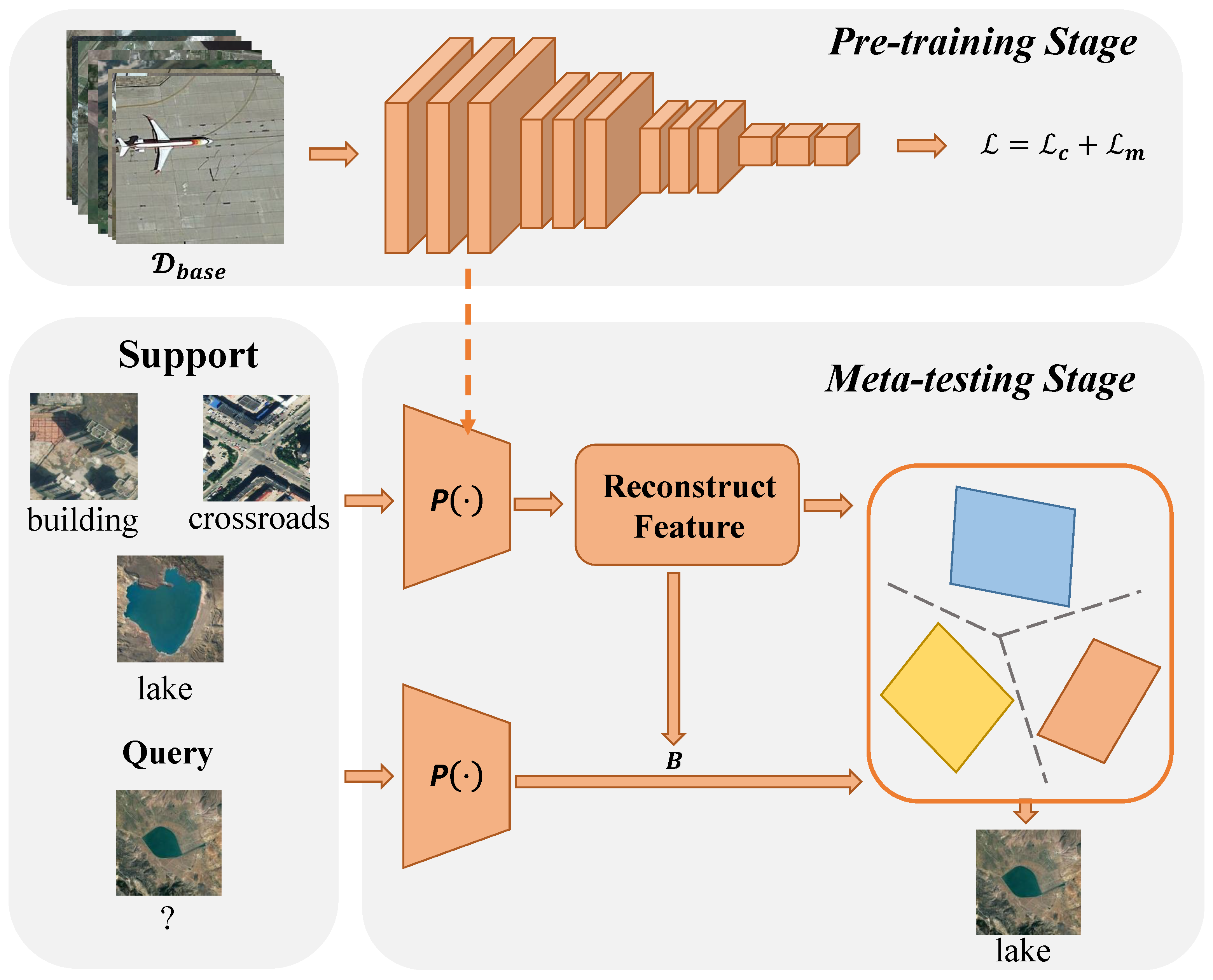
4.1. Overview Framework of the Proposed Method

This work applies the Class-Shared SparsePCA for the few-shot remote sensing scene classification, named CSSPCA. Figure 1 shows the steps of our proposed method. Specifically, different from the training method of the feature extractor in [20], we do not use the meta-learning method to train the feature extractor. Instead, we train the feature extractors following [39], which is more effective than the complex meta-learning algorithm. In our opinion, compared with the general few-shot image classification tasks, the few-shot remote sensing scene classification tasks have less data volume. When the convolutional neural network is trained, it is easy for the network to be over-fitted, resulting in worse generalization ability and affecting the final classification effect. We introduce self-supervised learning in the pre-training stage to improve the generalization ability of feature extractor by constructing more self-supervised data.

At the same time, it will inevitably bring new problems. Since the sample categories used by the pre-trained model are different from the remote sensing images, it is challenging for the feature extractor trained in the pre-trained stage to adapt to novel data, and there is the problem of “negative transfer”. To alleviate this problem, we propose using the Class-Shared SparsePCA maps novel data embedding features to obtain more discriminative space and more discriminative reconstructed features, thus alleviating the “negative transfer” problem and improving the performance of the few-shot remote sensing scene classification task.

4.2. Feature Extractor

In this work, we use Resnet-12 [40] as our backbone to classify all categories of data in ${\mathcal{D}}_{base}$, illustrated in Figure 2. The feature extractor consists of four residual blocks and dropout, $5\times 5$ average pooling and a fully connected (FC) layer. Each block contains $3\times 3$ convolution layers, batch normalization layers, and LeakyReLU layers, and $2\times 2$ max-pooling layers. We resize all the data to $84\times 84$ before training.

Figure 2. Schematic diagram of self-supervised auxiliary loss.

In the pre-training stage, we train the feature extractor by introducing a self-supervised method. The loss function $\mathcal{L}$ contains classification loss [41] ${\mathcal{L}}_c$ and auxiliary rotation loss [42] ${\mathcal{L}}_m$. ${\mathcal{L}}_c$ can be formulated as:

$$\begin{array}{c}\hfill {\mathcal{L}}_c=-\sum _c{y}_{(c,x)}log\left(p_{(c,x)}\right)\end{array}$$

(1)

where c denotes the $c_{th}$ class, $y_{(c,x)}$ indicates the truth label and $p_{(c,x)}$ is the probabilities that predicted the label of $x_{th}$ sample belonging to $c_{th}$ class. Then, we flip each sample to m, and $m=\{horizontally,vertically,diagonally\}$ is the label of the sample rotated by different angles. ${\mathcal{L}}_m$ can be formulated as:

$$\begin{array}{c}\hfill {\mathcal{L}}_m=-\sum _m{y}_{(m,x)}log\left(p_{(m,x)}\right)\end{array}$$

(2)

where $y_{(m,x)}$ indicates the truth label, and $p_{(m,x)}$ indicates the probabilities that predicted the label of $x_{th}$ sample belonging to $m_{th}$ class. The loss function is defined as follows:

$$\begin{array}{c}\hfill \mathcal{L}={\mathcal{L}}_c+{\mathcal{L}}_m\end{array}$$

(3)

In the meta-testing stage, we remove the FC layer of the pre-trained feature extractor and finally obtain a 512-dimensional embedding feature as the input of the classifier.

4.3. Class-Shared SparsePCA Classifier

To solve the problem of negative transfer in the few-shot remote sensing scene classification, we propose a novel method. We propose to use Class-Shared SparsePCA to project samples into subspace to obtain more discriminative reconstruction features and make them more suitable for few-shot remote sensing scene classification. The objective function is defined as follows:

$$\begin{array}{cc}\hfill argmi{n}_{A,B}& {∥X-XB{A}^T∥}_F^2+{\lambda }_0{∥B∥}_F^2+{\lambda }_1\sum _{j=1}^K{∥B_{•j}∥}_1+\eta {∥Y-XBW∥}_F^2\hfill \\ \hfill s.t.& A^{T}A=I_{K\times K},{∥W_{k•}∥}_2\le 1\hfill \end{array}$$

(4)

Here, we assume that $X\in {\mathbb{R}}^{N\times D}$, $A\in {\mathbb{R}}^{D\times K}$ and $B\in {\mathbb{R}}^{D\times K}$ denote the features extracted from the noval data, the synthesis dictionary (orthogonal matrix) and the analysis dictionary (sparse matrix), respectively. N is the number of features, D represents the dimension of features, and K is the dictionary size. $Y\in {\mathbb{R}}^{N\times C}$ represents the label matrix, and $W\in {\mathbb{R}}^{K\times C}$ denotes the classification plane, where C is the number of categories of sample X. $B_{•j}$ denotes the $j_{th}$ column of matrix B, and $W_{k•}$ denotes the $k_{th}$ row of matrix W. $\lambda$ and $\eta$ are constant.

If we initialize the synthesis dictionary A and the analysis dictionary B with random matrices with unit Frobenius norm [43], Equation (4) can be solved with the following three steps:

(i) Fix A and B; update W. The objective function is as follows:

$$f\left(W\right)=argmi{n}_{A,B}{∥Y-XBW∥}_F^{2}s.t.{∥W_{k•}∥}_2\le 1$$

(5)

We set $S=XB$, and $D=S^{T}S$, where $S\in {\mathbb{R}}^{N\times K}$, and $D\in {\mathbb{R}}^{K\times K}$. Then, we obtain the W as (6):

$$W_{k•}=\frac{{\left(S^{T}Y\right)}_{k•}-\left({\tilde{D}}_{k•}\right)W}{{∥{\left(S^{T}Y\right)}_{k•}-\left({\tilde{D}}_{k•}\right)W∥}_2}$$

(6)

where $\tilde{D}$ is D whose diagonal element is set to 0, and ${\left(S^{T}Y\right)}_{k•}$ denotes the $k_{th}$ row of matrix $S^{T}Y$.

(ii) Fix W and B; update A. The objective function is written as follows:

$$f\left(A\right)=argmi{n}_{A,B}{∥X-XB{A}^T∥}_F^{2}s.t.A^{T}A=I_{K\times K}$$

(7)

The problem can be soved by the SVD algorithm. We obtain the SVD as follows:

$$X^{T}XB=UD{V}^T$$

(8)

where $U\in {\mathbb{R}}^{D\times D}$, $D\in {\mathbb{R}}^{D\times K}$ and $V\in {\mathbb{R}}^{D\times K}$ are the matrices obtained by the SVD algorithm, and U and V are the unitary matrices.

Then, we obtain the synthesis dictionary A as Equation (9).

$$A=U{V}^T$$

(9)

(iii) Fix W and A; update B. The objective function is written as follows:

$$f\left(B\right)=argmi{n}_{A,B}{∥X-XB{A}^T∥}_F^2+{\lambda }_0{∥B∥}_F^2+{\lambda }_1\sum _{j=1}^K{∥B_{•j}∥}_1+\eta {∥Y-XBW∥}_F^2$$

(10)

Then, Equation (10) factorizes to Equation (11) as follows:

$$\begin{array}{c}\hfill f\left(B\right)=trace\left\{X^{T}X-2X^{T}XB{A}^T+A{B}^T{X}^{T}XB{A}^T\right\}+{\lambda }_{0}trace\left\{B^{T}B\right\}\\ \hfill +{\lambda }_1\sum _{j=1}^K{∥B_{•j}∥}_1+\eta trace\left\{Y^{T}Y-2Y^{T}XBW+W^T{B}^T{X}^{T}XBW\right\}\end{array}$$

(11)

Rewrite the objective function as follows:

$$\begin{array}{c}\hfill f\left(B\right)=trace\left\{B^T(X^{T}X+{\lambda }_{0}I)B+\eta W{W}^T{B}^T{X}^{T}XB\right\}\\ \hfill -2trace\left\{X^{T}XB{A}^T+\eta Y^{T}XBW\right\}+{\lambda }_1\sum _{j=1}^K{∥B_{•j}∥}_1\end{array}$$

(12)

Define $g\left(B\right)=trace\left\{·\right\}-2trace\left\{·\right\}$. The objective can be rewritten as follows:

$$f\left(B\right)=g\left(B\right)+{\lambda }_1\sum _{j=1}^K{∥B_{•j}∥}_1$$

(13)

According to Equation (13), we obtain that

$$f\left(B_{•k}\right)=g\left(B_{•k}\right)+{\lambda }_1{∥B_{•k}∥}_1$$

(14)

so that we can use the ADMM algorithm (Alternating Direction Method of Multipliers) [44] method to solve this problem:

$$\begin{array}{c}\hfill f(B_{•k},z)=g\left(B_{•k}\right)+{\lambda }_1{∥z∥}_{1}s.t.B_{•k}=z\end{array}$$

(15)

$$f(B_{•k},z,\xi )=g\left(B_{•k}\right)+{\lambda }_1{∥z∥}_1+{\xi }^T(B_{•k}-z)+\rho {∥B_{•k}-z∥}_2^2$$

(16)

where $\xi$ is the Lagrange multiplier and $\rho$ is constant.

Then, fix z and $\xi$; update the analysis dictionary $B_{•k}$

$$f\left(B_{•k}\right)=g\left(B_{•k}\right)+{\xi }^T{B}_{•k}+\rho {∥B_{•k}-z∥}_2^2$$

(17)

To this end, the optimal B can be formulated as:

$$B_{•k}={\left[G\right]}^{-1}\left[X^{T}X{A}_{•k}+\eta X^{T}Y{W}_{•k}^T+\rho z-\frac{\xi }{2}-\eta X^{T}X{\tilde{Z}}_{k•}\right]$$

(18)

where $G=\eta X^{T}X({\sum }_{j=1}^k{\left(W{W}^T\right)}_{kk})+X^{T}X+(\lambda +\rho )I$, $Z=W{W}^T$ and ${\tilde{Z}}_{k•}=\left\{\begin{array}{c}{Z}_{•p},p\ne k\hfill \\ 0,p=k\hfill \end{array}\right\}$.

Fix $B_{•k}$ and $\xi$; update z.

$$z=max\left\{B_{•k}+\frac{1}{2\rho }(\xi -{\lambda }_1),0\right\}+min\left\{B_{•k}+\frac{1}{2\rho }(\xi +{\lambda }_1),0\right\}$$

(19)

Fix $B_{•k}$ and z; update $\xi$.

$$\xi =\xi +\rho (B_{•k}-z)$$

(20)

4.4. Classification Scheme

Given a query image $x_q$, we extract its feature embedding $\mathcal{F}\left(x_q\right)$. The predicted label is obtained by Equation (21):

$$category\left(x_q\right)=max\left\{x_{q}AW\right\}$$

(21)

5. Experiments and Results

5.1. Datasets

We train feature extraction models on the few-shot learning datasets miniimagenet and tieredimagnet, respectively, and test them on two datasets: NWPU-RESISC45 and RSD46-WHU. Figure 3 shows several images of the datasets, and the details of these datasets are introduced as follows.

Figure 3. Samples from different datasets. (a) NWPU-RESISC45, (b) RSD46-WHU.

The NWPU-RESISC45 dataset is a dataset for remote sensing scene classification. It consists of 31,500 images divided into 45 classes of scenes. Each class contains 700 images with $256\times 256$ pixel size. As the split division setting proposed by [32], we divided the 45 scene classes into 25, 8, 12 for meta-training, meta-validation and meta-testing, respectively.

The RSD46-WHU is an open dataset for remote sensing scene classification. There are 117,000 images divided into 46 classes of scenes in the dataset, each with 500–3000 images of 256-pixel size. On the basis of [32], we separated it into three sections: 26 classes for meta-training, 8 classes for meta-validation and 12 classes for meta-testing. The specific information is shown in Table 1.

Table 1. NWPU-RESISC45 and RSD46-WHU dataset category information.

Dataset	All	Meta-Training	Meta-Validation	Meta-Testing
NWPU-RESISC45	45	25	8	12
RSD46-WHU	46	26	8	12

5.2. Implementation Details

In the pre-trained stage, we adopt a common Resnet-12 network for which the structure is same as [40], and the feature extractor trained on the server consists of eight Tesla-V100 GPU with 32 GB memory. In the course of training, the optimizer for the model is a stochastic gradient descent (SGD) optimizer. The momentum of the optimizer is set to $0.9$, and the weight decay is $1\times {10}^{-4}$. In addition, the learning rate was $0.1$ initially, then the learning rate was changed to $0.01$, $0.001$ and $0.0001$ at epochs 30, 60 and 90, respectively. The whole model consists of 120 pre-trained epochs on base data. Moreover, some standard data enhancement methods such as horizontal flipping, random clipping, and color dithering were applied before the data were fed into feature extractor. When the training is completed, the best model is chosen according to the classification precision testing on the meta-training set.

In the meta-testing stage, it is similar to common few-shot image classification. First, all remote sensing images are resized into $84\times 84$ for the whole dataset. Then, the parameters of the pre-trained feature extractor are fixed, and the last FC layer is removed. We can thus obtain a 512-dimensional feature vector for each remote sensing image through the feature extractor Resnet-12. Next, the CSSPCA classifier is used for classification. For the parameter for the CSSPCA, we fix ${\lambda }_0$ to $2^0$, ${\lambda }_1$ to $2^{-9}$, and $\rho$ to $2^{-3}$ on NWPU-RESISC45 dataset as well as ${\lambda }_0$ to $2^0$, ${\lambda }_1$ to $2^{-8}$, and $\rho$ to $2^{-10}$ on RSD46-WHU dataset under the 5-way 1-shot and 5-way 5-shot case. According to the few-shot learning experimental setting proposed by [20], we evaluate the method’s performance on the on N-way K-shot case over 600 episodes with 15 query samples. We randomly select N classes samples from the test samples for each episode and randomly select K samples for each class, where $N=5$ and $K=1$ or 5. Figure 4 shows the example of a 5-way 1-shot case with 600 episodes.

Figure 4. The example of a 5-way 1-shot case.

5.3. Experimental Results

The methods based on meta-learning such as [32,33,35] and others have gained excellent results, which has effectively solved the problem that the network is accessible to over-fitting due to fewer data. However, the network cannot be fully trained, making it difficult to further improve the accuracy of sample classification. Therefore, we proposed the method based on decision fusion to settle it effectively. At the same time, the decision fusion is applied to deal with the cross-domain negative transfer, which has achieved remarkable performance in the few-shot remote sensing scene classification.

We listed the experimental results of average accuracy (%) with $95\%$ confidence interval over 600 epochs in Table 2 and Table 3, respectively. The prior work experimental results come from their report. We usually test the accuracy of few-shot remote sensing scene classification under 5-way 1-shot and 5-way 5-shot cases. In the 5-way 1-shot case, only one image in each category is used to train the classifier, which is challenging.

Table 2. The few-shot classification accuracies on the NWPU-RESISC45 with $95\%$ confidence intervals over 600 epochs.

Method	Backbone	5-Way 1-Shot	5-Way 5-Shot
LLSR [45]	ConV-4	$51.43$	$72.90$
MAML [27]	ConV-4	$53.52\pm 0.83$	$71.69\pm 0.63$
ProtoNet [20]	ConV-4	$51.17\pm 0.79$	$74.58\pm 0.56$
RelationNet [46]	ConV-4	$57.10\pm 0.89$	$73.55\pm 0.56$
MatchingNet [34]	Conv-5	$37.61$	$47.10$
Meta-SGD [47]	ConV-5	$60.63\pm 0.90$	$75.75\pm 0.65$
DLA-MatchNet [33]	ConV-5	$68.80\pm 0.70$	$81.63\pm 0.46$
MAML [27]	Resnet-12	$56.01\pm 0.87$	$72.94\pm 0.63$
ProtoNet [20]	Resnet-12	$62.78\pm 0.85$	$80.19\pm 0.52$
RelationNet [46]	Resnet-12	$55.84\pm 0.88$	$75.78\pm 0.57$
TADAM [48]	Resnet-12	$62.25\pm 0.79$	$82.36\pm 0.54$
MetaOptNet [21]	Resnet-12	$62.72\pm 0.64$	$80.41\pm 0.41$
DSN-MR [49]	Resnet-12	$66.93\pm 0.51$	$81.67\pm 0.49$
D-CNN [14]	Resnet-12	$36.00\pm 6.31$	$53.60\pm 5.34$
MetaLearning [32]	Resnet-12	$69.46\pm 0.22$	$84.66\pm 0.12$
TPN [50]	Resnet-12	$66.51\pm 0.87$	$78.50\pm 0.56$
MKN [51]	Resnet-12	$65.84\pm 0.89$	$82.67\pm 0.55$
TAE-Net [52]	Resnet-12	$69.13\pm 0.83$	$82.37\pm 0.52$
Ours	Resnet-12	$\mathbf{71}.\mathbf{27}\pm \mathbf{0}.\mathbf{70}$	$\mathbf{85}.\mathbf{64}\pm \mathbf{0}.\mathbf{46}$

Table 3. The few-shot classification accuracies on the RSD46-WHU with $95\%$ confidence intervals over 600 epochs.

Method	Backbone	5-Way 1-Shot	5-Way 5-Shot
LLSR [45]	ConV-4	$51.43$	$72.90$
MAML [27]	ConV-4	$52.73\pm 0.91$	$69.18\pm 0.73$
ProtoNet [20]	ConV-4	$52.57\pm 0.89$	$71.95\pm 0.71$
RelationNet [46]	ConV-4	$55.18\pm 0.90$	$68.86\pm 0.71$
MAML [27]	Resnet-12	$54.36\pm 1.04$	$69.28\pm 0.81$
ProtoNet [20]	Resnet-12	$60.53\pm 0.99$	$77.53\pm 0.73$
RelationNet [46]	Resnet-12	$53.73\pm 0.95$	$69.98\pm 0.74$
TADAM [48]	Resnet-12	$65.84\pm 0.67$	$82.79\pm 0.58$
MetaOptNet [21]	Resnet-12	$62.05\pm 0.76$	$82.60\pm 0.46$
DSN-MR [49]	Resnet-12	$66.53\pm 0.70$	$82.74\pm 0.54$
D-CNN [14]	Resnet-12	$30.93\pm 7.49$	$58.93\pm 6.14$
MetaLearning [32]	Resnet-12	$69.08\pm 0.25$	$84.10\pm 0.15$
Ours	Resnet-12	$\mathbf{70}.\mathbf{61}\pm \mathbf{0}.\mathbf{73}$	$\mathbf{84}.\mathbf{50}\pm \mathbf{0}.\mathbf{48}$

Our method achieved 71.27% on the NWPU-RESISC45 dataset in the 5-way 1-shot case, and 85.64% in the 5-way 5-shot case, respectively. In the 5-way 1-shot case, we achieved an accuracy of 70.61% on the RSD46-WHU dataset in the 5-way 1-shot case, and 84.50% in the 5-way 5-shot case, respectively. Compared with the prior work, we have improved 0.98% and 0.40% on all datasets on the 5-way 5-shot case, respectively. Even on the 5-way 1-shot case, we attained 1.81% and 1.53%, respectively.

We summarize and analyze all few-shot remote sensing scene classification methods, of which ProtoNet, RelationNet, MatchingNet, DLA-MatchNet, TADAM, MetaOptNet, DSN-MR and MetaLearning are few-shot remote sensing scene classification methods based on metric learning, and LLSR, MAML and Meta-SGD are based on optimization. At the same time, the MetaLearning methods achieved the best performance on all datasets. We analyze that the method based on metric learning is more suitable for few-shot remote sensing scene classification.

We observed that prototypical networks and MAML methods performed much better when using Resnet-12 than ConV-4 on the NWPU-RESISC45 datasets. In particular, the prototypical network improved by $11.61\%$ and $5.61\%$, respectively, under the 5-way 1-shot and 5-way 5-shot cases. It can be seen that the more layers of the neural network, the better performance of extracted sample features. At the same time, we also observed that in the NWPU-RESISC45 dataset, the performance of most methods using Resnet-12 as the feature extractor was generally lower than that of the DLA-Matchnet method. We believe that the training data of remote sensing data were insufficient, resulting in the over-fitted problem of Resnet-12 during training.

5.4. Ablation Studies

5.4.1. Influence of Self-Supervised Mechanism

In the pre-training phase, a self-supervised mechanism is used to train the feature extractor. The mirror transformation is applied to the training samples and jointly constructs the loss function. We explain self-supervised auxiliary loss and give the effect on the final result to prove that the self-monitoring mechanism is better.

We flip the image, and generating the corresponding pseudo-label is used as an auxiliary classification task to supervise the network training to complete the image angle prediction task. Figure 2 is the schematic diagram of the self-supervised auxiliary loss. Suppose the network wants to predict the flip angle of the image. In that case, it must learn to understand the salient objects in the image, identify their orientation and object type, and then associate the object orientations with the original image. If the network cannot learn to understand these concepts, it cannot accurately predict flip angles. At the same time, the construction of auxiliary tasks increases the training complexity of the network to a certain extent. The features extracted by the network can be classified well and accurately predict the flip angle. The features extracted during the training process have better generalization.

We test the self-supervised learning mechanism on the NWPU-RESISC45 and RSD46-WHU datasets. The test results are shown in Table 4. baseline is the result of baseline without self-supervised mechanism. $baseline+ssm$ is the result of baseline with self-supervised mechanism. All experiments are performed under the same settings.

Table 4. Comparison results with $baseline$ on 5-way few-shot case.

Weight	NWPU-RESISC45		RSD46-WHU
	1-Shot	5-Shot	1-Shot	5-Shot
$baseline$	$66.04\pm 0.82$	$82.50\pm 0.52$	$67.89\pm 0.79$	$82.76\pm 0.52$
$baseline+ssm$	$71.27\pm 0.70$	$85.64\pm 0.46$	$70.61\pm 0.73$	$84.50\pm 0.48$

From Table 4, we can see that under the different test cases of the two datasets, using the self-supervision mechanism is better than the results of the $baeline$. Compared with the results of the data augmentation method based on rotation, using the self-supervision mechanism improved $5.23\%$ and $2.72\%$ in all datasets on the 5-way 1-shot case, and it promoted $3.14\%$ and $1.74\%$ on the 5-way 5-shot case, respectively.

We plot the changes in the training and validation accuracy of the first 50 epoch trainings on base data (left side) and self-supervised data (right side) using the self-supervised mechanism on NWPU-RESISC, as shown in Figure 5. The figure on the left shows the variation in accuracy of the main classification task for training and validation on the base data. With the increase in the frequency of training, the training and validation accuracy have been increasing simultaneously. After training to 15 epochs, the training and verification accuracy gradually stabilized at about 94%. The figure on the right shows the variation in accuracy of the auxiliary classification task trained and verified on self-supervised data. The accuracy of the training is significantly improved at first. When the training stage reaches the four epoch, the training accuracy begins to stabilize and remains at about 70%, while the verification accuracy fluctuates. Notably, when we adjusted the learning rate from 0.1 to 0.01 in the 30th epoch, the validation accuracy did not change significantly, but the training accuracy displayed a tiny but distinct improvement, which exists in both cases.

Figure 5. Change in training accuracy in pre-training stage, (a) shows training accuracy on base data, and (b) shows training accuracy on self-supervised data.

5.4.2. Influence of Reconstructive Feature

At present, there is a “negative transfer” problem in few-shot remote sensing scene classification, and the feature extractor pre-training on base data cannot adapt well to the features of novel data. We proposed to use Class-Shared SparsePCA to learn and reconstruct features. We performed ablation experiments to verify the validity of the reconstructed features. We use t-SNE (t-distributed Stochastic Neighbor Embedding) [53] to visualize novel data features X and reconstructed features $XB$ on NWPU-RESISC45, and the experimental results are shown in Figure 6. It can be seen from the figure that the distributions of the novel data’s different category features overlap each other. In contrast, the reconstructed features have a closer distance between the same category features and a longer distance between different category features, which has better discrimination and is more conducive to image classification.

Figure 6. The t-SNE visualization. We use t-SNE to perform visual analysis on the extracted novel data features and the reconstructed features. (a) shows t-SNE result on novel data features, and (b) shows t-SNE result on reconstructed features.

5.4.3. Influence of Parameters

We carry out ablation studies to analyze the influence of the hyper-parameters ${\lambda }_0$, ${\lambda }_1$ and $\rho$. To determine the optimal parameters of the experiment more quickly, we fixed two of the parameters and then changed another parameter. The experimental results on NWPU-RESISC45 and RSD46-WHU under the 5-way 1-shot case are shown in Figure 7, Figure 8 and Figure 9. Finally, we choose the parameter with the best classification result as our final parameter.

Figure 7. Influences of parameters ${\lambda }_0$. (a) shows experimental results on NWPU-RESISC45, and (b) shows experimental results on RSD46-WHU.

Figure 8. Influences of parameters ${\lambda }_1$. (a) shows experimental results on NWPU-RESISC45, and (b) shows experimental results on RSD46-WHU.

Figure 9. Influences of parameters $\rho$. (a) shows experimental results on NWPU-RESISC45, and (b) shows experimental results on RSD46-WHU.

5.4.4. Influence of Meta-Testing SHOT

Table 2 and Table 3 illustrate that the heterogeneity in performance between 5-way 1-shot and 5-shot cases is noteworthy. We further develop the effects of various shots on performance in the 5-way setting. As we can see from Figure 10, the performance of our approach gradually rose as the number of shots increased, but at a slower rate, especially in the 5-way 2-shot case.

Figure 10. Ablation studies to show the performances of the meta-testing shot. (a) shows experimental results on NWPU-RESISC45, and (b) shows experimental results on RSD46-WHU.

6. Conclusions

In recent years, the few-shot remote sensing scene classification has attracted researchers’ attention, and it solves the lack of available training data. We have analyzed the methods on few-shot remote sensing scene classification in recent years and found two problems. One is that the inappropriate neural network model can easily lead to trained over-fitting or can be unable to extract the deep representation features of samples. The other is that the pre-trained model with a better feature extraction ability will have the problem of negative transfer due to the massive difference between the pre-trained data used in training and remote sensing data. In response to these questions, we propose a few-shot scene classification method based on Class-Shared SparsePCA, aiming at the existing problems. First, we propose using self-supervised learning as an auxiliary classification task, which helps us train a more robust feature extractor with limited data. We propose a new and more robust classifier for few-shot remote sensing scene classification in the meta-test phase, which can effectively improve the discrimination of novel data features. We have significantly improved the performance of two commonly used few-shot remote sensing scene classification datasets. Through many ablation experiments, we proved the rationality and effectiveness of our proposed method.

References

1. Zhu, Q.; Wu, W.; Xia, T.; Yu, Q.; Yang, P.; Li, Z.; Song, Q. Exploring the Use of Google Earth Imagery and Object-Based Methods in Land Use/Cover Mapping. Remote Sens. 2013, 5, 6026–6042. [Google Scholar]
2. Johnson, B.A. Scale Issues Related to the Accuracy Assessment of Land Use/Land Cover Maps Produced Using Multi-Resolution Data: Comments on “The Improvement of Land Cover Classification by Thermal Remote Sensing”. Remote Sens. 2015, 7(7), 8368–8390. Remote Sens. 2015, 7, 13436–13439. [Google Scholar] [CrossRef] [Green Version]
3. Zhu, Q.; Zhong, Y.; Zhao, B.; Xia, G.S.; Zhang, L. Bag-of-visual-words scene classifier with local and global features for high spatial resolution remote sensing imagery. IEEE Geosci. Remote Sens. 2016, 13, 747–751. [Google Scholar] [CrossRef]
4. Cheng, H.F.; Zhang, W.B.; Chen, F. Advances in researches on application of remote sensing method to estimating vegetation coverage. Remote Sens. Land Resour. 2008, 1, 13–17. [Google Scholar]
5. Bechtel, B.; Demuzere, M.; Stewart, I.D. A Weighted Accuracy Measure for Land Cover Mapping: Comment on Johnson et al. Local Climate Zone (LCZ) Map Accuracy Assessments Should Account for Land Cover Physical Characteristics that Affect the Local Thermal Environment. Remote Sens. 2019, 12, 1769. [Google Scholar] [CrossRef]
6. Ghorbanzadeh, O.; Blaschke, T.; Gholamnia, K.; Meena, S.R.; Tiede, D.; Aryal, J. Evaluation of different machine learning methods and deep-learning convolutional neural networks for landslide detection. Remote Sens. 2019, 11, 196. [Google Scholar] [CrossRef] [Green Version]
7. Solari, L.; Del Soldato, M.; Raspini, F.; Barra, A.; Bianchini, S.; Confuorto, P.; Nicola Casagli, N.; Crosetto, M. Review of satellite interferometry for landslide detection in Italy. Remote Sens. 2020, 12, 1351. [Google Scholar] [CrossRef]
8. Manfreda, S.; McCabe, M.F.; Miller, P.E.; Lucas, R.; Pajuelo Madrigal, V.; Mallinis, G.; Ben Dor, E.; Helman, D.; Estes, L.; Ciraolo, G. On the use of unmanned aerial systems for environmental monitoring. Remote Sens. 2018, 10, 641. [Google Scholar] [CrossRef] [Green Version]
9. Połap, D.; Włodarczyk-Sielicka, M.; Wawrzyniak, N. Automatic ship classification for a riverside monitoring system using a cascade of artificial intelligence techniques including penalties and rewards. ISA Trans. 2021, 12, 232–239. [Google Scholar]
10. Połap, D.; Włodarczyk-Sielicka, M. Classification of Non-Conventional Ships Using a Neural Bag-Of-Words Mechanism. Sensors 2020, 20, 1608. [Google Scholar] [CrossRef] [Green Version]
11. Zhang, W.; Tang, P.; Zhao, L. Remote sensing image scene classification using CNN-CapsNet. Remote Sens. 2019, 11, 494. [Google Scholar] [CrossRef] [Green Version]
12. Zou, Q.; Ni, L.; Zhang, T.; Wang, Q. Deep learning based feature selection for remote sensing scene classification. IEEE Geosci. Remote Sens. Lett. 2015, 12, 2321–2325. [Google Scholar] [CrossRef]
13. Hu, F.; Xia, G.S.; Hu, J.; Zhang, L. Transferring deep convolutional neural networks for the scene classification of high-resolution remote sensing imagery. Remote Sens. 2015, 7, 14680–14707. [Google Scholar] [CrossRef] [Green Version]
14. Cheng, G.; Yang, C.; Yao, X.; Guo, L.; Han, J. When deep learning meets metric learning: Remote sensing image scene classification via learning discriminative CNNs. IEEE Trans. Geosci. Remote Sens. 2018, 56, 2811–2821. [Google Scholar] [CrossRef]
15. Cheng, G.; Han, J.; Lu, X. Remote sensing image scene classification: Benchmark and state of the art. Proc. IEEE 2017, 105, 1865–1883. [Google Scholar] [CrossRef] [Green Version]
16. Jegou, H.; Perronnin, F.; Douze, M.; Sánchez, J.; Perez, P.; Schmid, C. Aggregating local image descriptors into compact codes. IEEE Trans. Pattern Anal. Mach. Intell. 2011, 34, 1704–1716. [Google Scholar] [CrossRef] [Green Version]
17. Yang, Y.; Newsam, S. Bag-of-visual-words and spatial extensions for land-use classification. In Proceedings of the 18th SIGSPATIAL International Conference on Advances in Geographic Information Systems, San Jose, CA, USA, 2–5 November 2010; pp. 270–279. [Google Scholar]
18. Xu, K.; Huang, H.; Li, Y.; Shi, G. Multilayer feature fusion network for scene classification in remote sensing. IEEE Geosci. Remote Sens. Lett. 2020, 17, 1894–1898. [Google Scholar] [CrossRef]
19. Wang, J.; Liu, W.; Ma, L.; Chen, H.; Chen, L. IORN: An effective remote sensing image scene classification framework. IEEE Geosci. Remote Sens. Lett. 2018, 15, 1695–1699. [Google Scholar] [CrossRef]
20. Snell, J.; Swersky, K.; Zemel, R. Prototypical networks for few-shot learning. Adv. Neural Inf. Process. 2017, 30, 4077–4087. [Google Scholar]
21. Lee, K.; Maji, S.; Ravichandran, A.; Soatto, S. Meta-learning with differentiable convex optimization. In Proceedings of the IEEE Conference on Computer Vision and Pattern Recognition, Long Beach, CA, USA, 16–20 June 2019; pp. 10657–10665. [Google Scholar]
22. Shao, S.; Xing, L.; Xu, R.; Liu, W.F.; Wang, Y.J.; Liu, B.D. MDFM: Multi-Decision Fusing Model for Few-Shot Learning. IEEE Trans. Circuits Syst. Video Technol. 2021. [Google Scholar] [CrossRef]
23. Xing, L.; Shao, S.; Liu, W.F.; Han, A.X.; Pan, X.S.; Liu, B.D. Learning Task-specific Discriminative Embeddings for Few-shot Image Classification. Neurocomputing 2022, 488, 1–3. [Google Scholar] [CrossRef]
24. Tian, Y.; Wang, Y.; Krishnan, D.; Tenenbaum, J.B.; Isola, P. Rethinking few-shot image classification: A good embedding is all you need? In Proceedings of the Computer Vision—ECCV 2020: 16th European Conference, Glasgow, UK, 23–28 August 2020; pp. 266–282. [Google Scholar]
25. Zou, H.; Hastie, T.; Tibshirani, R. Sparse principal component analysis. J. Comput. Graph. Stat. 2006, 15, 265–286. [Google Scholar] [CrossRef] [Green Version]
26. Abdi, H.; Williams, L.J. Principal component analysis. WIley Interdiscip. Rev. Comput. Stat. 2010, 2, 433–459. [Google Scholar] [CrossRef]
27. Finn, C.; Abbeel, P.; Levine, S. Model-agnostic meta-learning for fast adaptation of deep networks. In Proceedings of the 34th International Conference on Machine Learning, Sydney, Australia, 6–11 August 2017; Volume 70, pp. 1126–1135. [Google Scholar]
28. Rajeswaran, A.; Finn, C.; Kakade, S.M.; Levine, S. Meta-Learning with Implicit Gradients. In Proceedings of the Advances in Neural Information Processing Systems 33, Vancouver, BC, Canada, 6–12 December 2020; pp. 113–124. [Google Scholar]
29. Zhou, P.; Yuan, X.T.; Xu, H.; Yan, S.; Feng, J. Efficient meta learning via minibatch proximal update. In Proceedings of the Advances in Neural Information Processing Systems 33, Vancouver, BC, Canada, 6–12 December 2020; pp. 1534–1544. [Google Scholar]
30. Alajaji, D.A.; Alhichri, H. Few shot scene classification in remote sensing using meta-agnostic machine. In Proceedings of the 2020 6th Conference on Data Science and Machine Learning Applications, Riyadh, Saudi Arabia, 4–5 March 2020; pp. 77–80. [Google Scholar]
31. Alajaji, D.; Alhichri, H.S.; Ammour, N.; Alajlan, N. Few-shot learning for remote sensing scene classification. In Proceedings of the 2020 Mediterranean and Middle-East Geoscience and Remote Sensing Symposium, Tunis, Tunisia, 9–11 March 2020; pp. 81–84. [Google Scholar]
32. Zhang, P.; Bai, Y.; Wang, D.; Bai, B.; Li, Y. Few-shot classification of aerial scene images via meta-learning. Remote Sens. 2021, 13, 108. [Google Scholar] [CrossRef]
33. Li, L.; Han, J.; Yao, X.; Cheng, G.; Guo, L. DLA-MatchNet for few-shot remote sensing image scene classification. IEEE Trans. Geosci. Remote 2020, 99, 1–10. [Google Scholar] [CrossRef]
34. Vinyals, O.; Blundell, C.; Lillicrap, T.; Wierstra, D. Matching networks for one shot learning. Proc. Adv. Neural Inf. Process. Syst. 2016, 29, 4077–4087. [Google Scholar]
35. Yuan, Z.; Huang, W. Multi-attention DeepEMD for Few-Shot Learning in Remote Sensing. In Proceedings of the IEEE 9th Joint International Information Technology and Artificial Intelligence Conference, Chongqing, China, 11–13 December 2020; pp. 1097–1102. [Google Scholar]
36. Zhang, C.; Cai, Y.; Lin, G.; Shen, C. Deepemd: Few-shot image classification with differentiable earth mover’s distance and structured classifiers. In Proceedings of the IEEE Conference on Computer Vision and Pattern Recognition, Seattle, WA, USA, 14–19 June 2020; pp. 12203–12213. [Google Scholar]
37. Dvornik, N.; Schmid, C.; Mairal, J. Diversity with cooperation: Ensemble methods for few-shot classification. In Proceedings of the IEEE Conference on Computer Vision and Pattern Recognition, Long Beach, CA, USA, 15–21 June 2019; pp. 3723–3731. [Google Scholar]
38. Yue, Z.; Zhang, H.; Sun, Q.; Hua, X.S. Interventional Few-Shot Learning. Adv. Neural Inf. Process. Syst. 2020, 33, 2734–2746. [Google Scholar]
39. Shao, S.; Xing, L.; Wang, Y.; Xu, R.; Zhao, C.Y.; Wang, Y.J.; Liu, B.D. Mhfc:Multi-head feature collaboration for few-shot learning. In Proceedings of the 2021 ACM on Multimedia Conference, Chengdu, China, 20–24 October 2021. [Google Scholar]
40. Wang, Y.; Xu, C.; Liu, C.; Zhang, L.; Fu, Y. Instance credibility inference for few-shot learning. In Proceedings of the IEEE Conference on Computer Vision and Pattern Recognition, Seattle, WA, USA, 14–19 June 2020; pp. 12836–12845. [Google Scholar]
41. Rubinstein, R. The Cross-Entropy Method for Combinatorial and Continuous Optimization. Methodol. Comput. Appl. Probab. 1999, 1, 127–190. [Google Scholar] [CrossRef]
42. Xing, L.; Shao, S.; Ma, Y.T.; Wang, Y.J.; Liu, W.F.; Liu, B.D. Learning to Cooperate: Decision Fusion Method for Few-Shot Remote Sensing Scene Classification. IEEE Geosci. Remote Sens. Lett. 2022, 19, 1–5. [Google Scholar] [CrossRef]
43. Horn, R.A.; Johnson, C.R. Matrix Analysis; Cambridge University Press: Cambridge, UK, 2012. [Google Scholar]
44. Boyd, S.; Parikh, N.; Chu, E.; Peleato, B.; Eckstein, J. Distributed optimization and statistical learning via the alternating direction method of multipliers. Found. Trends Mach. Learn. 2011, 3, 1–122. [Google Scholar]
45. Zhai, M.; Liu, H.; Sun, F. Lifelong learning for scene recognition in remote sensing images. IEEE Geosci. Remote Sens. Lett. 2019, 16, 1472–1476. [Google Scholar] [CrossRef]
46. Sung, F.; Yang, Y.; Zhang, L.; Xiang, T.; Torr, P.H.; Hospedales, T.M. Learning to compare: Relation network for few-shot learning. In Proceedings of the IEEE Conference on Computer Vision and Pattern Recognition, Salt Lake City, UT, USA, 18–22 June 2018; pp. 1199–1208. [Google Scholar]
47. Li, Z.; Zhou, F.; Chen, F.; Li, H. Meta-sgd: Learning to learn quickly for few-shot learning. arXiv 2018, arXiv:1707.09835. [Google Scholar]
48. Oreshkin, B.; Rodríguez López, P.; Lacoste, A. TADAM: Task dependent adaptive metric for improved few-shot learning. In Proceedings of the Advances in Neural Information Processing Systems 31, Long Beach, CA, USA, 4–9 December 2017; pp. 719–729. [Google Scholar]
49. Simon, C.; Koniusz, P.; Nock, R.; Harandi, M. Adaptive Subspaces for Few-Shot Learning. In Proceedings of the IEEE Conference on Computer Vision and Pattern Recognition, Seattle, WA, USA, 14–19 June 2020; pp. 4136–4145. [Google Scholar]
50. Liu, Y.; Lee, J.; Park, M.; Kim, S.; Yang, E.; Hwang, S.J.; Yang, Y. Learning to Propagate Labels: Transductive Propagation Network for Few-shot Learning. In Proceedings of the International Conference on Learning Representations, Vancouver, BC, Canada, 30 April–3 May 2018. [Google Scholar]
51. Cui, Z.; Yang, W.; Chen, L.; Li, H. MKN: Metakernel networks for few shot remote sensing scene classification. IEEE Trans. Geosci. Remote Sens. 2022, 60, 4705611. [Google Scholar] [CrossRef]
52. Zhang, P.; Fan, G.; Wu, C.; Wang, D.; Li, Y. Task-Adaptive Embedding Learning with Dynamic Kernel Fusion for Few-Shot Remote Sensing Scene Classification. Remote Sens. 2021, 13, 4200. [Google Scholar] [CrossRef]
53. Van der Maaten, L.; Hinton, G. Visualizing Data using t-SNE. J. Mach. Learn. Res. 2008, 9, 2579–2605. [Google Scholar]
Publisher’s Note: MDPI stays neutral with regard to jurisdictional claims in published maps and institutional affiliations.
Article Metrics
Citations
Article Access Statistics
Multiple requests from the same IP address are counted as one view.