Article

RID—Roof Information Dataset for Computer Vision-Based Photovoltaic Potential Assessment

Department of Mechanical Engineering, Institute of Automotive Technology, TUM School of Engineering and Design, Technical University of Munich, Boltzmannstraße 15, 85748 Garching bei München, Germany
*
Author to whom correspondence should be addressed.
Remote Sens. 2022, 14(10), 2299; https://doi.org/10.3390/rs14102299
Submission received: 22 March 2022 / Revised: 3 May 2022 / Accepted: 5 May 2022 / Published: 10 May 2022

Abstract

:
Computer vision has great potential to accelerate the global scale of photovoltaic potential analysis by extracting detailed roof information from high-resolution aerial images, but the lack of existing deep learning datasets is a major barrier. Therefore, we present the Roof Information Dataset for semantic segmentation of roof segments and roof superstructures. We assessed the label quality of initial roof superstructure annotations by conducting an annotation experiment and identified annotator agreements of 0.15–0.70 mean intersection over union, depending on the class. We discuss associated the implications on the training and evaluation of two convolutional neural networks and found that the quality of the prediction behaved similarly to the annotator agreement for most classes. The class photovoltaic module was predicted to be best with a class-specific mean intersection over union of 0.69. By providing the datasets in initial and reviewed versions, we promote a data-centric approach for the semantic segmentation of roof information. Finally, we conducted a photovoltaic potential analysis case study and demonstrated the high impact of roof superstructures as well as the viability of the computer vision approach to increase accuracy. While this paper’s primary use case was roof information extraction for photovoltaic potential analysis, its implications can be transferred to other computer vision applications in remote sensing and beyond.

Graphical Abstract

1. Introduction

Climate change is one of the greatest global challenges of our time and requires prompt and effective action. The transition from fossil to renewable energy generation is an essential contributor to reducing greenhouse gas emissions. Photovoltaic (PV) power is a major pillar of the renewable energy mix. Artificial intelligence and computer vision (CV) can support and accelerate the introduction and operation of PV systems [1,2]. For example, CV can improve load forecasting by detecting cloud formations and enhance solar irradiation prediction [3,4]. CV is also used for mapping existing solar panels, which are often unknown to grid operators [5,6,7,8,9,10]. The focus of this paper lies on extracting roof information for estimating unexploited rooftop PV potential, which represents an important basis for decisions by policy-makers or investors. While deep learning CV approaches have recently proven effective for mapping solar panels on a large scale [5,6,7], there are only a few publications applying the same approaches to extracting further roof information for rooftop PV potential assessment. A major challenge is the lack of adequate datasets for deep learning. To the best of our knowledge, there is only one publicly available dataset for the semantic segmentation of roof segments [11] and none for roof superstructures. Therefore, this paper aimed to advance CV-based semantic segmentation of roof information in aerial images in three steps as visualized by Figure 1. First, we present the Roof Information Dataset (RID) for roof segments and roof superstructures. Second, we examine the annotation quality of roof superstructures and its influence on neural networks’ training and prediction. Third, we assess the viability and benefit of using CV-based roof superstructure detection for PV potential analysis.
The rest of the paper is structured as follows. Section 2 derives the necessity of roof information data for semantic segmentation based on the application of PV potential analysis in Section 2.1. Subsequently, related work on assessing dataset quality and the effect of noisy data on deep learning is described in Section 2.2 and Section 2.3. Based on the presented publications, research gaps and contributions are presented in Section 2.4. After introducing the dataset in Section 3.1, three methods for examining annotation quality, for training and evaluating the neural networks as well as for PV potential analysis are outlined in Section 3.2. Similar to the methods, the results in Section 4 are structured into annotation quality, neural network results, and PV potential. Section 5 discusses the results and limitations of the work, and Section 6 concludes the paper.

2. Related Work

This section briefly introduces state-of-the-art PV potential assessments, the role of CV in this field as well as associated publicly available CV datasets. Then, we review the challenges of determining dataset quality in remote sensing and cover related work on implications of data quality for CV. Finally, we summarize the related work and derive this paper’s contributions.

2.1. PV Potential Based on Aerial Images

LiDAR vs. CV-Based approaches: Rooftop PV potential assessment aims at accurately calculating the PV potential of each roof while also being scalable to a city or a larger region. Light detection and ranging (LiDAR) approaches are the state of the art with respect to the level of detail of the input data [12]. Such an assessment is based on three-dimensional data and, therefore, allows for a highly accurate calculation of the irradiation on a tilted plane as well as shading analysis. LiDAR-based approaches have been the subject of multiple studies [13,14,15,16,17] and have been applied in solar cadasters over the last decade, e.g., Mapdwell [18], Google’s Project Sunroof [19], and tetraeder.solar [20]. However, a downside is that flat roof superstructures (windows or existing solar panels) or small superstructures (chimneys) usually remain undetected. In practice, those superstructures significantly limit panel placement options, leading to the overestimation of PV potential [21,22]. Furthermore, even though LiDAR data are becoming increasingly available, there is still no exhaustive coverage, especially in less densely populated areas. Therefore, researchers are conducting PV potential analyses based on alternative methods for extracting roof information using CV and aerial images.
Lack of Datasets for CV-Based Approaches: Existing CV-based publications extract building footprints [23] or determine roof segments including their azimuth orientation [11,24,25,26]. Although various authors have already shown that CV can be effectively used to detect solar panels in satellite images on a large scale [5,6,7], only a few studies have explored detecting the whole range of superstructures on a roof.
Mainzer et al. [25] used conventional CV techniques to extract roof segments and roof superstructures. Additionally, they used a deep learning approach for PV panel detection and excluded roofs with installed PV systems from their potential assessment. Lee et al. [11] presented DeepRoof, a semantic segmentation CNN for determining roof segments and their orientation. Krapf et al. [26] built upon the work by Lee et al. [11] and increased the level of detail by adding a semantic segmentation CNN for roof superstructures.
Deep learning and CV applications have become a major research interest in the remote sensing community, but the availability of annotated images has been identified as one of the biggest challenges in this field [27,28]. While there are multiple datasets on building footprint segmentation [29,30,31], a dataset on the semantic segmentation of roof segments [11], and datasets on solar panel detection [8,32], there is no publicly available deep learning dataset for the semantic segmentation of roof superstructures. To the best of our knowledge, there is only one roof superstructure dataset from the city of Geneva [33]. The data include partial annotations of roof superstructures, but the labels are too irregular and inaccurate for training CNNs.

2.2. Dataset Quality

Challenge of Determining Ground Truth in Remote Sensing: In remote sensing, the quality of ground truth used to train machine learning models has been an issue for at least 25 years [34,35]. However, inadequate datasets remain an unsolved challenge [27]. Most datasets in remote sensing are sourced from human annotators [27]. Thus, they are subject to human interpretation [36] and inter- and intra-annotator variability [37,38]. Depending on the task, labeling can be complex, even for domain experts [39,40]. Identifying objects’ boundaries on aerial images is challenging, because for some objects, spatial boundaries may be more or less well defined [41,42]. For example, there is no clearly defined line between a forest and a field. Even objects with well-defined boundaries, such as buildings, can be challenging to accurately delineate due to the limited image resolution [43]. Nevertheless, possible quality concerns in human-labeled ground truth are often neglected and data are implicitly treated as error free [36,44,45,46]. A recent review by Elmes et al. [45] on training data error in machine learning applications for earth observation calls for the field to investigate their data quality more rigorously and to openly report on it. Determining the accuracy of a labeled ground truth dataset requires reference data. In remote sensing, reference data are scarce and, in some cases, impossible to acquire [35,47]. Since a ground truth dataset is typically larger than its corresponding reference dataset, an overall accuracy score represents an extrapolated estimation [48]. Hence, the composition of the reference data sample can skew the extrapolation and lead to errors in the accuracy assessment [49,50].
Agreement Instead of Accuracy: As an alternative to measuring accuracy using a reference dataset, some authors measure annotator certainty or annotator agreement by comparing the labels of multiple annotators [32,44,51,52,53]. The ability of humans to annotate objects in aerial images is object-class dependent [36,54,55]. Van Coillie et al. [36] studied internal and external factors affecting the annotation quality of annotators delineating objects in aerial imagery. They found that the internal factor speed and the external factor distractedness have the largest influence, respectively. Albrecht studied human annotator agreement for object classes including buildings, roads, gardens, and forests [55]. Their study showed that labels of multiple annotators on the same image revealed varying levels of disagreement. In an analysis of the PV array annotations in their dataset, Bradbury et al. [32] found that approximately 30% of arrays are missed by one of the two annotators. Additionally, some objects are mistaken for PV arrays, and arrays delineated by both annotators have a median intersection over union (IoU) of 0.86.

2.3. Learning from Noisy Data

Although noisy data and its effects on algorithms have been a topic for over 30 years [56], machine learning practitioners commonly focus on improving the model while neglecting the quality of the data [45,57]. However, data quality influences a model’s achievable performance, the validity of its performance evaluation, and its success in the real world [45,57]. The ratio of mislabeled data in real-world image classification datasets is reported to range from 8.0% to 38.5% [58,59,60,61,62].
Mellor et al. [63] studied the effects of different ratios of mislabeled data in combination with training set size on the accuracy of a land cover classifier. They showed that for binary classification, increasing the training dataset size can mostly mitigate even the negative effect of 25% mislabeling. For multiclass classification, more data only slightly improves performance. Swan et al. [64] studied the influence of three different types of training set data noise on the performance of a SegNet for building segmentation in aerial imagery. They investigate shifted labels, omitted labels, and added false labels and found that all the three types negatively impacted the F1 score. However, they also found that some may have positive effects on either precision or recall. Shifted labels lead to a loss of edge detail. Omitted labels lead to a large increase in precision and reduction in recall, because the network predicts fewer positive labels. Lastly, added false labels only lead to small decreases in the metrics.
A publication by Northcutt et al. [65] found pervasive label errors in the test sets of popular datasets, most notably a label inaccuracy of 5.85% in ImageNet. They further found that a model architecture which performed best on a noisy test set was inferior to the actual clean test set.

2.4. Summary and Contributions

Our literature review shows that there is currently only one publicly available dataset for the semantic segmentation of roof segmentations and no publicly available dataset for the semantic segmentation of roof superstructures. Furthermore, it showed that manually annotated labels are prone to errors such as misclassification, omission, or spatial inaccuracy. Quantifying such errors is challenging because of the absence of highly accurate reference data. Even though annotation errors can have a great effect on training and evaluation, the quality of the datasets is often neglected. To improve the model performance, researchers commonly take a model-centric approach instead of a data-centric approach. Therefore, this paper contributes to the research gap of using CV for PV potential assessment by addressing the lack of datasets for extracting roof information from aerial images with deep learning. We included a label quality assessment and investigated the effect of class-specific label quality on the training and evaluation of a U-Net. The paper includes the following contributions:
  • The paper provides two semantic segmentation datasets for 1880 buildings: one for roof segments and one for roof superstructures. The Roof Information Dataset (RID) is made available as georeferenced geometries and as ground truth image masks as well as in two states of annotation quality—initial labels, and reviewed labels. This enables a greater variety of data-centric experimentation for future research;
  • For smaller datasets, high label quality is important. Using an annotation experiment, we investigated the level of difficulty of labeling roof superstructures. Furthermore, with the experiment, we provide an approach for the challenging task of quantifying annotation quality in the absence of reference data and applied it on the initial dataset;
  • The annotation quality has implications for the training as well as the evaluation of a CNN. Therefore, this paper includes a detailed analysis of the predictions by a U-Net and compared the class-specific labeling performance of annotators and U-Net;
  • Roof superstructures decrease the PV potential significantly. Using the trained network, we estimated the PV potential for a study area and discuss the necessity of identifying roof superstructures.

3. Materials and Methods

To structure our research, we derived three hypotheses. Superstructure annotation is a challenging labeling task due to the fact of their small size and ambiguous segmentation boundaries. Therefore, we expected a low mean IoU between labelers (Hypothesis 1). Increased label quality can improve network performance posing the question, if the network becomes as good as human labelers, who annotate the initial dataset (Hypothesis 2)? Finally, we aimed at testing the viability of the network’s predictions on the application of PV potential analysis. Neglecting roof superstructures leads to overestimation of PV potential, as existing superstructures decrease the available roof area. Therefore, including this information should improve the PV potential assessment (Hypothesis 3).
Hypothesis 1.
Annotation agreements approximately reach a value of 0.5 mean IoU between labelers during the initial labeling step;
Hypothesis 2.
Using the reviewed dataset of higher quality, the trained network can achieve similar performances as the human annotators’ initial labels, that is, close to the 0.5 mean IoU;
Hypothesis 3.
Including superstructures mapped by CV decreases overestimation of PV potential by approximately 20%.
Section 3 is organized accordingly. First, RID and its key metrics are described in Section 3.1. Then, Section 3.2 presents the methods for investigating the hypotheses, covering the annotation experiment (Section 3.2.1), training and evaluation of CNNs (Section 3.2.2), and PV potential analysis (Section 3.2.3).

3.1. Materials

Section 3.1.1 describes the RID and its annotation process, and Section 3.1.2 gives an overview of the dataset’s key indicators. The RID can be downloaded at: doi.org/10.14459/2022mp1655470. Additionally, code for evaluating the dataset or adapting masks can be downloaded at: https://github.com/TUMFTM/RID (accessed on 21 March 2022).

3.1.1. Dataset Description

The RID contains semantic labels of roof segments and roof superstructures. The images are aerial images that were downloaded via the Google Maps API [66] and which can be used for research purposes. Our goal was to create a dataset of approximately 2000 buildings within one connected area. Detecting small roof superstructures, such as chimneys or windows, requires very high-resolution images. Therefore, we chose aerial images instead of satellite images. Furthermore, we aimed at using images of challenging quality with respect to contrast, shadow, and distortion to enable a better transferability to other regions. Thus, we selected the rural German village of Wartenberg as our study area. The available images in this area had a resolution of approximately 10 cm/pixel but were less sophisticated than high-quality images in more urban regions.
Annotation Process: The annotation process of RID was conducted in two phases. First, the initial labeled dataset was created by five university members using a self-developed tool that allowed for drawing polygon and line labels on a Google Maps Dynamic API interface. The rule set underlying the annotation process was published together with the dataset. While our tool facilitated georeferenced labeling and provided a good overview of geographic coverage, the magnification factor of the images was limited. Due to the ambiguity of the segmentation boundaries of some superstructure classes, such as ladders, trees, shadows, and small-sized objects in the image, we conducted a second review step. To this end, we used the Computer Vision Annotation Tool (CVAT) [67], because it enables better administration of the reviewing task and at a higher zoom. We conducted the review phase after the annotation experiment described in Section 3.2.1 and some initial training to apply our findings to the quality improvement. The review was performed on each image by two labelers, who did not contribute to the initial dataset to reduce bias. With this paper, we published the initial as well as the reviewed dataset. By this, we aimed to enable future research on the effects of label quality improvement and to promote data-centric CV approaches.
Published Dataset: RID consists of three components: aerial images, georeferenced vector data, and masks. The dataset includes one aerial image for each annotated building, with the building at its center. Second, we provide the annotated labels as tables of georeferenced geometries. Furthermore, RID contains the training, validation, and test masks that are derived from the geometry labels and prepared for the deep learning pipeline. The respective code was published alongside the dataset.
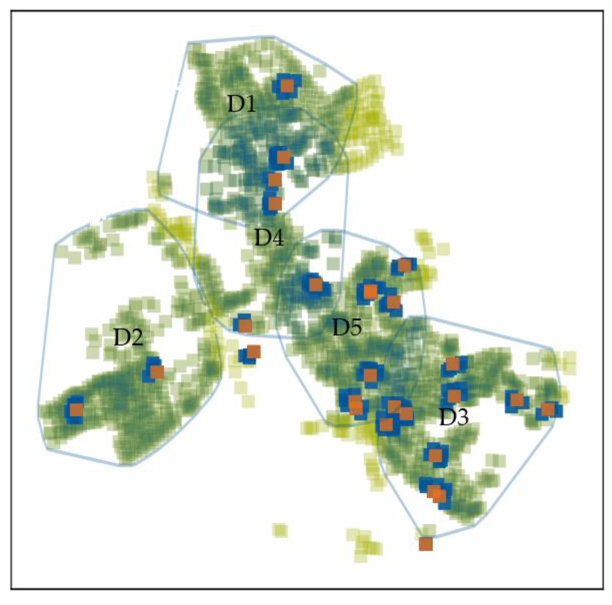
Dataset Split: Using roof-centered images requires special preparation of training, validation, and test sets. A random data split leads to overlapping training and test images and, consequently, overestimated test metrics. Therefore, we split the dataset with respect to geographic location. Figure 2 illustrates the image boundaries of our dataset.
The annotation experiment explained in Section 3.2.1 used 26 buildings (orange). In this paper, we used the same buildings to form the test dataset. Hence, we excluded all images from the training and validation set that intersected with the building outline (dark blue). Then, we created five training and validation sets by iteratively increasing the buffer (blue lines) around a coordinate until the validation set size was 20% of all images. We refer to the dataset configurations as north (D1), west (D2), east (D3), center north (D4), and center south (D5).

3.1.2. Dataset Key Indicators

The RID contains 1880 annotated roofs. The images cover an area of 1.5 km2, excluding overlap, and 4.9 km2 in total.
Roof Segment Metrics: The roof segment annotations include 4520 polygons, and its classes were derived by its azimuths. Lee et al. [11] selected 16 azimuth classes, for example, south, south–south–west, and south–west, plus a class for flat roofs and one for trees. Usually, roof orientations are biased towards north, south, east, and west for architectural reasons. Therefore, we provided code to classify roof segments in three different ways.
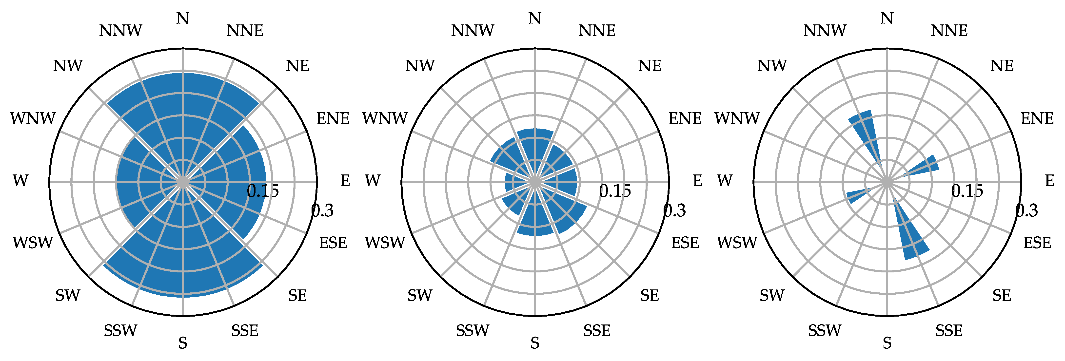
Figure 3 visualizes the class distribution of the respective roof segment masks using 4, 8, or 16 azimuth classes. Classes were unbalanced for the 16 classes, but the level of detail decreased for the four classes, as the category “south” contained azimuth angles between 45° and −45°.
Superstructure Metrics: In addition, we labeled 12,359 superstructure polygons. The goal was to annotate all pixels on a roof that were different from the roof’s surface. To this end, we defined eight roof superstructure classes, which can be allocated to structural objects (PV module, dormer, window, ladder, and chimney), natural objects (tree and shadow), or other objects with an unknown class. The class PV module contains photovoltaic and solar thermal panels. Unclassified superstructures were assigned to the unknown class. Although natural objects do not physically restrict the installation of new PV modules, we labeled these pixels, too, to be able to investigate whether the network can benefit from their annotation. Furthermore, they constituted a share of more than 20% of the labeled area as illustrated in Figure 4. The figure shows the class distribution of the roof superstructure labels by the number of labels and by area, indicating a class imbalance in the dataset. While labels in the “unknown” class were the most common by occurrence number, its mean area was smaller than the area of PV modules, dormers, and shadows. The number of PV module annotations was one of the smallest, but it was the largest class in terms of annotated area. Furthermore, the share of annotated roof superstructure pixels was only 4.12% in comparison to 93.88% background pixels. This underlines the challenge of this deep learning task.

3.2. Methods

To resolve the challenge of evaluating label quality in the absence of reference data with limited overhead, we defined an annotation experiment in Section 3.2.1. In Section 3.2.2, we described the training process for two neural network architectures that served to investigate the implications of the annotation agreement on the CNN. In the Section 3.2.3, the method of estimating PV potential is presented. For the rest of the paper, we focused on the roof superstructure dataset containing the initial labels or otherwise explicitly referred to the reviewed dataset. Code for training and evaluating CNNs can be downloaded at: https://github.com/TUMFTM/RID (accessed on 21 March 2022).

3.2.1. Evaluation of Annotator Agreement

Annotation Experiment Dataset: To assess Hypothesis 1, stating that superstructure annotation exhibits an agreement of 0.5 of the mean IoU between labelers, we conducted a labeling experiment. We created an auxiliary dataset based on 26 images that were each labeled by five annotators, who contributed to the initial labeled dataset. The auxiliary dataset was not used for training and validation of the CNNs, only for testing. It was gathered under similar conditions as the initial dataset to ensure comparability between the two datasets. To limit the necessary labeling time, the buildings were manually selected to contain at least 15 occurrences of each superstructure class in the 26 images. However, this introduced a different class balance in the auxiliary dataset than the highly imbalanced class distribution of the initial dataset (Figure 3). This fact was mitigated by using class-specific weights when transferring results from the annotation experiment to the entire initial dataset
Evaluation Metrics: The confusion matrix is a common tool in remote sensing accuracy assessments [50,68]. In this paper, we derived confusion matrices to calculate the annotator agreement by successively treating one annotated mask as ground truth and the others as predictions. For each image, each labeler was compared to all other labelers separately, leading to 20 confusion matrices per image and 520 for the entire experiment. We derived class-sensitive (multi-class) and class-agnostic agreements (superstructure vs. background) from the confusion matrix. Examples of two annotations are given in Figure 5. We calculated the averaged overall confusion matrix as a micro-average by summing up all absolute confusion values of the 520 matrices and normalizing them in the end. The macro-averaging approach normalizes each matrix first, before computing the sum of each entry. The differences between micro- and macro-averaging are discussed in detail in [69].
Furthermore, we used IoU, also known as the Jaccard index [70], to calculate the class-specific annotation agreement of labelers and define it as follows:
IoU   = TP TP + FP + FN
using true positives (TP), false positives (FP), and false negatives (FN). The mean IoU of one image was calculated as the mean of all class-specific IoUs including the background class. The overall reported mean IoU is the mean of all images’ class-specific mean IoUs, corresponding to a macro-averaged mean IoU.

3.2.2. Training and Evaluation of Neural Networks

Implementation Details: To compare the class-specific annotation agreement with a CNN and to answer Hypothesis 2, we trained a U-Net [71] and a Panoptic FPN [72]. We used an implementation as used in [73] and training details as given in Table 1. As we report our results using IoU, we chose Jaccard loss as the loss function. We added focal loss because of the class imbalance as recommended by Jadon [74].
Dataset Preparation: The dataset was constructed using the 1880 roof-centered aerial images described in Section 3.1.1. Our test set consisted of the same 26 buildings that were selected for the annotation experiment. Accordingly, 134 images were excluded from the training and validation set (see Figure 2) to assure zero geographical overlap of the images with the building. The remaining images were split five times into training (80%) and validation (20%) as illustrated in Figure 2. We conducted cross-validation and present our results for both networks as well as the initial and reviewed training and validation datasets.
Evaluation: We report the comparison between the CNN and human annotations by calculating the IoU for each building and by computing the confusion matrix as a sum of the confusion matrices of each building in a micro-averaging way as described in Section 3.2.1. The images’ mean IoUs were derived using macro-averaging of its class-specific mean IoUs, similar to the approach defined in Section 3.2.1. For comparison with the human annotations, the evaluation is conducted for the centered building only. This is required because the annotation experiment uses buildings scattered within the whole study area and focused on one building, neglecting other buildings in the image. Hence, detected superstructures of other surrounding buildings in the image, which were not part of the 26 buildings from the annotation experiment, were treated as background for ground truth and prediction. We trained 20 networks, a U-Net and a Panoptic FPN that were trained on initial and reviewed labels with five different training and validation splits (D1–D5), introduced in Section 3.1.1. A detailed analysis in Section 4.2 is presented for the network with the best performance on the test set.

3.2.3. PV Potential Estimation

PV Potential Estimation Method: To assess the relevance of superstructures for PV potential analysis and the viability of the deep learning approach (Hypothesis 3), the third part of this paper estimates the PV potential for a study area. The calculation procedure consisted of four steps:
  • Predict superstructures per roof segment;
  • Derive vectorized representation of the superstructures;
  • Calculate the PV system area and resulting peak power;
  • Estimate the yearly technical potential per roof segment.
In step 1, we used the trained network to predict superstructures on roofs. Step 2 transformed the superstructures from a raster format to georeferenced, vectorized format to facilitate the downstream potential estimation. Using roof segment boundaries, the usable PV area was calculated in step 3. To isolate the effect of superstructure detection, this paper used the ground truth for roof segments. The usable PV system area was determined by a PV module placement algorithm. Modules were placed in orientation of the segment’s azimuth and projected onto the horizontal plane with respect to the slope angle. Modules intersecting with superstructures are discarded. The algorithm places modules horizontally and vertically and chooses the alignment with the greater number of modules. Modules on flat roofs are assumed to be south oriented. The system peak power was calculated by summing up the modules’ peak power of 400 Wp each. We compared the module placement approach to an estimation that uses the roof segment area, subtracts the superstructure area, and assumes a specific peak power of 0.25 kWp/m2, which corresponds to modules of a size 1.6 × 1 m and 400 Wp. For flat roofs, the specific peak power is 0.125 kWp/m2 to account for the distance between module rows needed to avoid shading.
The final step 4, obtained the technical potential from the PVGIS [78] API to estimate the PV potential. PVGIS applied the r.sun model [79] for solar radiation modeling enabling calculations of large areas. A review comparing this method to other methods for solar potential estimation was published by Freitas et al. [80]. The technical potential was downloaded for one location in the study area, azimuth values in 3° steps, and a constant slope value of 30°. Furthermore, we selected data from the year 2014, because this year exhibited average yearly solar radiation compared to the data for all available years at PVGIS. A default PV system loss of 14% was assumed. As the approach is based on 2D information only, no shadow effects of surrounding buildings or superstructures were considered in this paper.
Dataset and Configurations: We derived the technical potential for each roof segment of 359 buildings in the validation dataset of the best network. In contrast to using the test dataset of the annotation experiment, we chose the validation dataset for two reasons. First, the roof superstructures were more representative because the annotation experiment roofs contained a higher-than-average number of superstructures for the purpose of our analysis. Second, the validation dataset consisted of a greater number of buildings. However, the validation dataset brings the disadvantage of predicting superstructures with higher accuracy than on an independent test set. Nevertheless, creating an additional test set for the PV potential analysis was not within the scope of this paper.

4. Results

4.1. Annotation Experiment

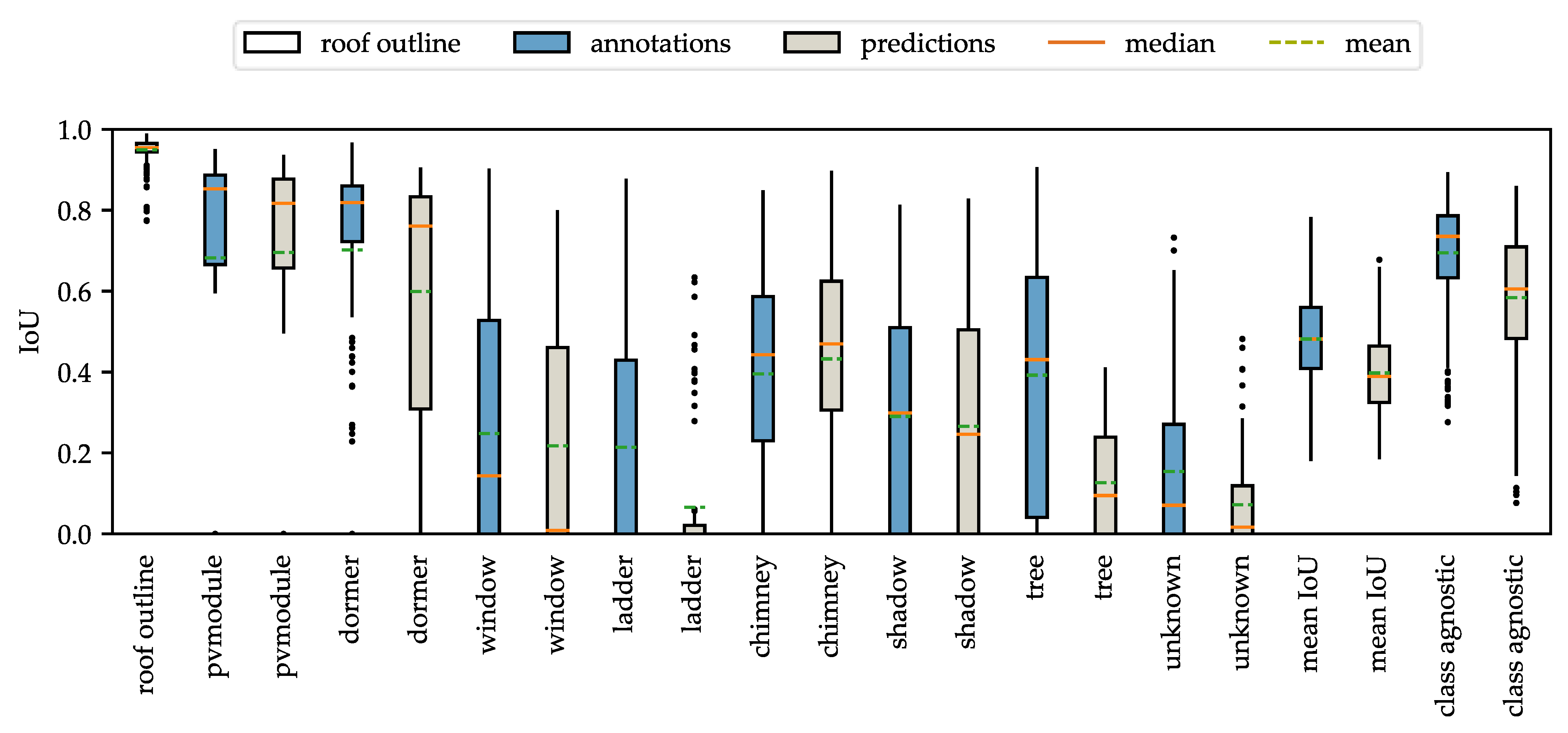
The results of the annotation experiment are illustrated as boxplots (blue) of the IoUs for all superstructure classes in Figure 6. The figure additionally includes the annotators’ IoUs of the roof outline as a reference (left boxplot, white). Furthermore, the IoUs of the U-Net’s predictions (gray), which are discussed in Section 4.2, are plotted next to the annotators IoUs to compare the two. On the right, the figure also shows the mean IoUs per image and the class-agnostic mean IoUs per image. The boxplots show that the participants’ agreement was strongly dependent on the superstructure class. For example, the annotators were very confident at delineating roofs, demonstrated by the high mean of 0.95 and a low variance. This matches the findings of Albrecht et al. [55]. In contrast, more ambiguous and challenging classes, such as shadows, tree, or unknown, exhibited means of 0.29, 0.39, and 0.15, respectively.
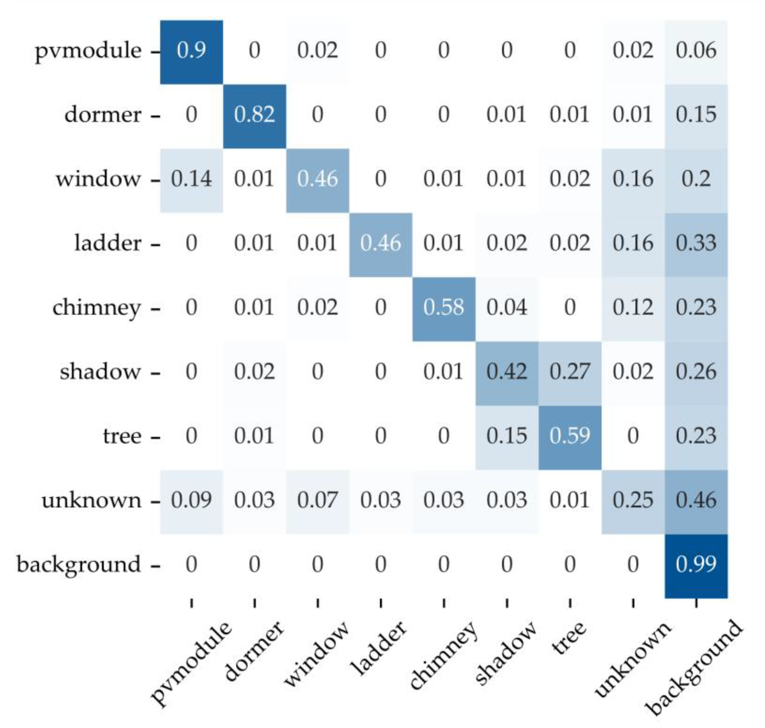
To discuss annotation agreement in more detail, Figure 7 contains the micro-averaged confusion matrix.
High Agreement: The annotators were confident labeling dormers (mean: 0.70, median: 0.83) and PV modules (mean: 0.68, median: 0.82—similar to [30]). They rarely confused dormers with other superstructures but omitted labeling approximately 15% of dormer pixels. This can be traced back to architectural edge cases where the semantic boundary between dormers and the roof area was unclear. The PV module class displayed the lowest confusion rate with the background class. Its only notable confusion rates with other superstructures came from windows and unknowns.
Low Agreement: Chimneys (mean: 0.39, median: 0.44), trees (mean: 0.39, median: 0.43), shadows (mean: 0.29, median: 0.30), windows (mean: 0.25, median: 0.14), ladders (mean: 0.22, median: 0.00), and unknowns (mean: 0.15, median: 0.07) were more challenging for humans to label consistently at the provided image resolution. At a median agreement value of 0.00, it can be concluded that labeling ladders as a separate class was too challenging for humans in most cases. In general, the thematic class agreement (diagonal) displayed in Figure 7 was low except for PV modules and dormers. However, the figure also shows that the class-agnostic agreement was significantly better. This can be seen from the relatively low confusion of the superstructure classes with roofs. Except for the unknown and PV module labels, all classes exhibited values between 0.15 and 0.30. This underlines the ambiguity of the unknown class and the clarity of the PV module labels.
Label Quality of the Initial Dataset: By weighting the class-specific IoUs with respect to their area (Figure 3), the metric can be transferred from the annotation experiment’s auxiliary dataset to the entire initial dataset with 1880 images. Hence, the estimated human label performance in terms of micro-averaged IoU was 0.52 for class-sensitive labeling and 0.71 for class-agnostic labeling. The difference between the two was a measure for the amount of misclassification, while the class-agnostic IoU indicated the spatial agreement.

4.2. Neural Networks

Results of Trained Networks: We conducted 20 training runs (two model architectures × two dataset states × five training-validation splits) and selected four models, two U-Nets and two Panoptic FPNs with the lowest loss value for the initial and reviewed dataset, respectively. The training–validation split D2 (Section 3.1.1) led to the lowest loss values for the U-Net trained on the initial labels, while the other three models showed the lowest loss for D1. The twelve models trained on D1, D2, and D4 resulted in similar loss values with a mean loss of 0.55. The eight training runs of training–validation splits D3 and D5 resulted in higher losses at a mean of 0.58, indicating a small geographic bias.
To compare the CNNs to the human annotators, the four selected models were applied on the annotation experiment test dataset, which contained 26 images with 130 ground truth masks (Table 2). The models showed mean IoUs of 0.42–0.44. Furthermore, the four models predicted the same 26 images with 26 ground truth masks from the reviewed dataset with higher IoUs of 0.45–0.46, even though two models were trained on initial labels and two models were trained on reviewed labels. This suggests that the higher IoUs came from more precise annotations in the reviewed test dataset and that the models can partly overcome inconsistencies in the initial training dataset. Furthermore, this underlines the significance of a high-quality test dataset.
Selection of Best Model: For the subsequent comparison to human annotations, we use a CNN trained on initial labels and chose U-Net, as it performed slightly better on the annotation experiment test set than the Panoptic FPN. The evaluation is conducted only on buildings that are part of the annotation experiment, as described in Section 3.2.2, while the rest of the image was set to background. To investigate the effect of this filtering, the U-Net was evaluated on the same images without a filter using masks from the original initial and reviewed dataset, containing 26 masks instead of 130 masks in the auxiliary dataset. Without a filter, the mean IoU was lower for the initial dataset (0.40 vs. 0.42) but increased for the reviewed dataset from 0.43–0.46. Hence, we concluded that the filtering did not lead to an unjustified boost, and the subsequent results can be transferred from the auxiliary to the original dataset.
Class-Specific Performance of U-Net: Figure 6 introduced in Section 4.1, compares the class-specific IoUs of annotators and the U-Net. The figure shows that the class-agnostic mean IoU of the U-Net trained on multiple classes reached 0.58, approximately 0.11 less than the value from the annotation experiment (0.69). The class-specific IoUs for PV modules (0.68 vs. 0.69), windows (0.25 vs. 0.22), and chimneys (0.39 vs. 0.43) were similar between human annotation and prediction, respectively. The prediction of ladders (0.21 vs. 0.06) or trees (0.39 vs. 0.12) varied significantly. However, both classes are less relevant for the PV potential analysis due to the low number of ladders on roofs and the fact that trees can be removed to increase solar radiation on a roof. The U-Net’s predictions of dormers achieved a high mean IoU of 0.60, although it displayed a high variance.
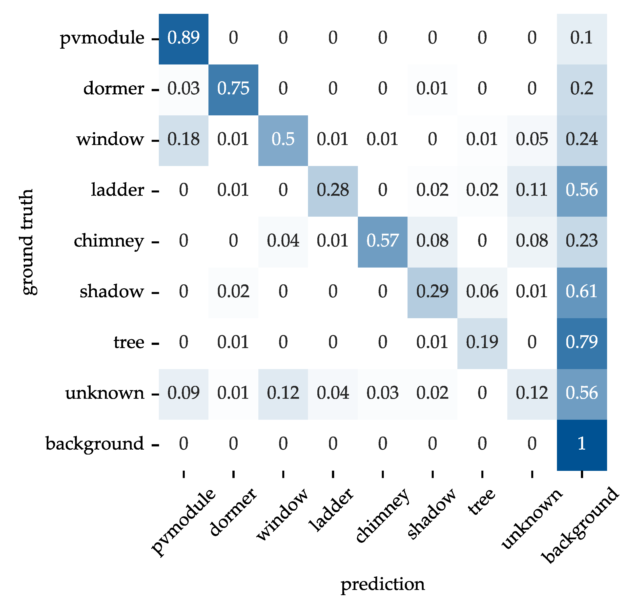
Figure 8 shows the confusion matrix of the U-Net. PV modules had the highest TP value of 0.89. As reflected in the mean IoUs, dormers, windows, and chimneys had higher TP values than the rest of the classes. Windows were confused with PV modules and the unknown class, and the reasons could be erroneous ground truth or false prediction. Furthermore, the U-Net predicted approximately 44% of unknown superstructures but assigned the correct class for only 12% of unknown ground truth. The U-Net’s confusion with background was highest for trees and shadows, indicating a lower performance for these two classes.
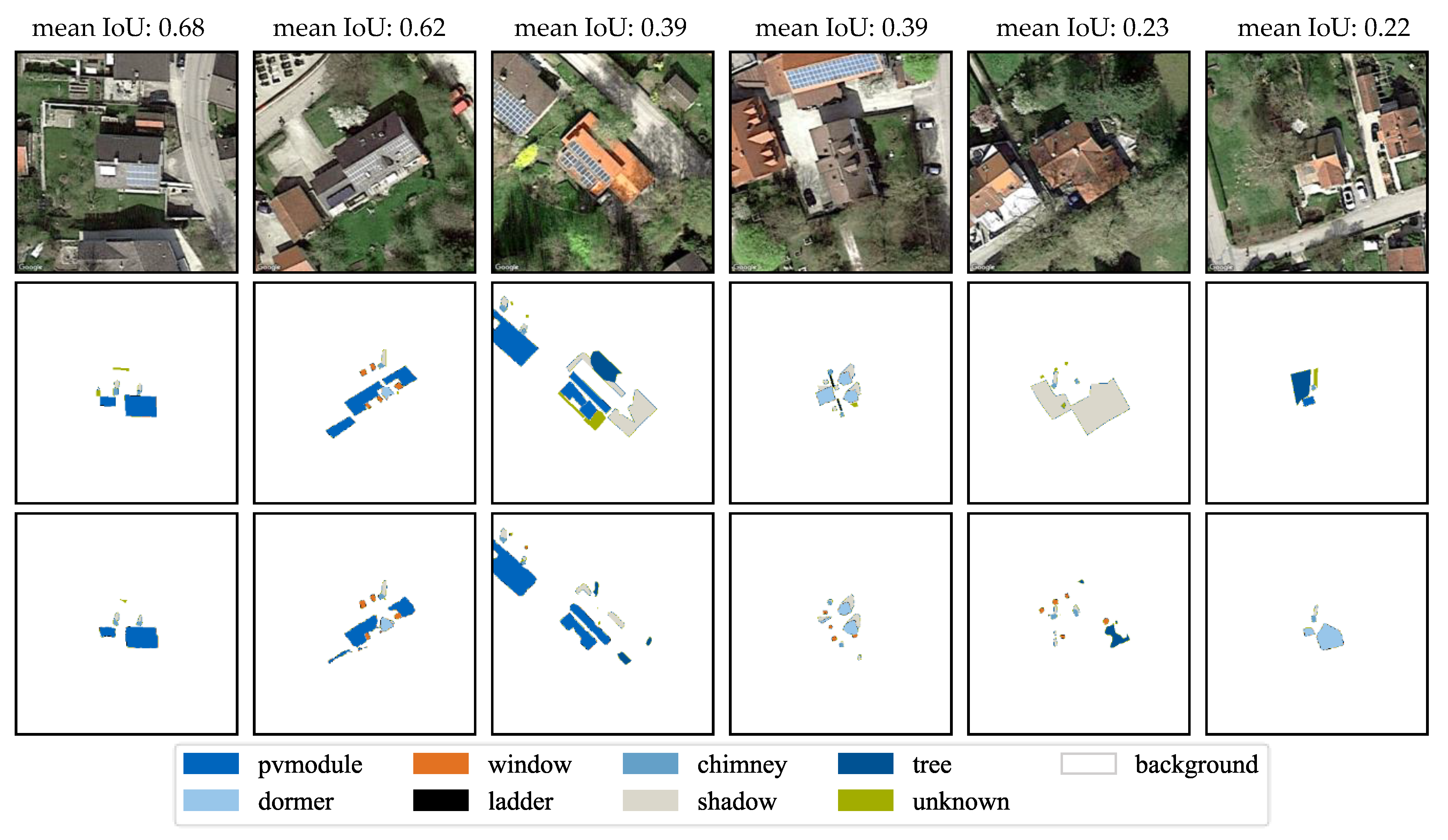
Prediction Examples: Figure 9 depicts six images with ground truth and prediction. From left to right, the images resemble the top two, median two, and bottom two predictions on the test set with respect to the network’s mean IoU.
In the top two images, the U-Net predicted PV modules, dormers, windows, and chimney wells. While the median two images showed good predictions of PV modules, dormers, and chimneys, and misclassification and the presence of trees and ladders led to lower mean IoUs. The predictions reached IoUs of 0.68 and 0.62, which are good as they are the highest annotation agreement on these images, respectively.
The bottom two images on the right contain fewer superstructures. They also underline the labeling challenge, because the second right image’s ground truth included a large ambiguous shadow label and windows labeled as unknown.
In the right-most image, the dormer is a borderline case due to the fact of its size, the roof is covered by a tree, and the shadow reached the outline of the roof, provoking an unclear classification between shadow and ladder.
The challenge of labeling images, such as the two right ones, underlines the difficulty of the annotation task for roof superstructures. Furthermore, it depicts the large influence of the test set on the evaluation of a CNN, because the predictions seem reasonable at first, or even outperform some of the classification decisions of the human annotator, e.g., the windows on the second right image.

4.3. PV Potential

This section presents the PV potential assessment for the validation dataset D2 using the U-Net discussed in Section 4.2. To investigate Hypothesis 3, we calculated the technical potential according to the approach described in Section 3.2.3 for six configurations using ground truth labels for the roof segments.
Effect of Superstructures: Figure 10 visualizes the results for the study area. The values are derived for each roof segment as specific energy generation in kWh/m2a to be able to compare roof segments of various sizes. Hence, a roof segment’s energy generation is divided by its entire area, not its usable area, for each configuration. Configuration one is the baseline, calculated under the assumption that the roof segment area equals the PV system area. The specific yearly energy generation is between 110 and 254 kWh/m2a depending on the segment’s azimuth orientation to the north or south, respectively. The total technical potential reached 14.76 GWh/a.
Configurations two and three included the ground truth and predictions of roof superstructures, and the mean specific yearly energy generation was 149 kWh/m2a and 169 kWh/m2a, respectively, corresponding to a reduction in the total estimated technical potential of 20.5% and 15.0%. The configuration using predicted superstructures displayed a higher potential due to the fact of less superstructure area in comparison to the ground truth. However, the difference was 0.82 GWh/a, demonstrating that the network can improve potential assessment despite relatively low IoUs.
Configuration four was calculated under the assumption that segments with existing solar arrays were not exploited for further PV installations, leading to a 29.5% lower technical potential. This underlines the significant impact of considering existing solar installations, especially in Germany, where residential solar systems have been installed for more than a decade.
PV Potential Using Module Placement: An increasingly realistic PV potential estimation is achieved in configurations five and six, which are based on placed modules. Placing modules on roof segments regardless of roof superstructures in configuration five exhibits a mean specific yearly energy generation of 108 kWh/m2a, 44.9% lower than the baseline configuration one. Configuration six shows the necessity of considering superstructures, as the mean specific yearly energy generation was 78 kWh/m2a, and the technical potential decreased by 31.1% to 7.04 GWh/a compared to configuration five. This decrease doubled the difference between configuration one and three, illustrating that locating superstructures is highly relevant for module placement. This finding was aggravated by the fact that modules placed in groups of less than four were usually not considered in real PV system design due to the high installation effort.
In addition, the effect of superstructures displayed a high variety. While on average, a roof segment’s specific energy generation was reduced by 25%, and the decrease was less than 5% for 39% and less than 15% for 50% of roof segments. At the same time, superstructures led to larger reductions of more than 20% for approximately 43% of roof segments, and 10% of segments experienced a decrease of 70% or higher.
Module Placement Examples: Figure 11 includes an exemplary visualization of roof segments and roof superstructures and placed modules for three images in the study area. The left image visualized the south-oriented modules on a flat roof that was partly covered with existing PV modules. The network did not detect the superstructure in between the PV modules and falsely placed isolated arrays in the middle. The center and right display modules placed in isolation or small groups to fill in gaps between superstructures. In practice, PV planners prefer coherent areas for PV systems, reducing the installed modules. Locating superstructures on roofs is one important advantage of aerial image-based PV potential analysis. However, the presented study assumed 30° for the roof slope of all tilted segments and considered no shadowing. Variances in slope can alter the outcome, and shadows further decrease the actual technical potential.

5. Discussion

Section 5 first discusses the hypotheses proposed in Section 2.4 and then points out the paper’s limitations.

5.1. Discussion of Hypotheses

Discussion of Hypothesis 1. The results in Section 4.1 confirm Hypothesis 1 and demonstrate the challenge of annotating small superstructures in high-resolution aerial images. The annotator agreement of initial labels reached a mean IoU of 0.48. Class-specific IoUs revealed significant differences reaching from a 0.70 for dormers to a 0.15 mean IoU for unknowns.
Discussion of Hypothesis 2. The results of Section 4.2 showed that networks trained on initial annotations and reviewed annotations performed similarly on the annotation experiment test set. Furthermore, the best network achieved a mean IoU of 0.44, which was 0.04 lower compared to the annotation agreement of 0.48. However, this was partly attributed to inexact initial labels in the annotation experiment as the networks performed better on the same 26 buildings using reviewed labels (0.45–0.46). Furthermore, the details in Figure 9 show that the top two predictions achieved IoU scores that were as high as the best annotations on the respective images and that the network can outperform the initial annotations in some cases. Nevertheless, Hypothesis 2 was rejected because the models’ IoUs did not reach 0.50.
In addition, based on the comparison of the best network’s predictions with the annotation experiment, we can draw two conclusions regarding the application of aerial image-based deep learning for PV potential assessment. First, while we included shadows and trees as superstructure classes for research purposes, these two classes should be excluded from datasets in the future. Second, a class-agnostic approach could be investigated, as spatial accuracy is more important than classification to determine PV potential accurately.
Discussion of Hypothesis 3. The study presented in Section 4.3 confirms Hypothesis 3, as superstructures reduced the technical potential by 20.5% in configurations one vs. three. The effect of superstructures was even higher when the PV potential was evaluated on placed modules and led to a decrease of 31.1% in configurations five vs. six. Furthermore, our analysis revealed that the effect of superstructures varied greatly between roof segments. Thirty-nine percent of segments were affected only by a 5% or lower reduction, while the decrease was higher than 20% for approximately 43% of segments. Hence, it is important to conduct roof segment-specific analysis of superstructure effects instead of using constant estimations of available roof area.

5.2. Limitations of the Work

The limitations of this work cover the three presented contents of the paper: the RID, its quality and implications on network training, as well as the PV potential analysis. Although RID covers 1880 unique buildings with more than 4500 roof segment and more than 12,000 roof superstructure labels, the study area was small and restricted to one town in a rural German setting. Therefore, we expect that the networks cannot be transferred to a broad range of roof architectures without expansion of the dataset. As a comparison, the DeepRoof dataset for roof segments contains 2274 buildings from six cities in the USA [11]. However, more than 90% of the buildings come from two cities, and the unique number of buildings is less than 2274 due to the fact of overlapping images.
In this paper, we estimated the label quality of initial annotations by conducting an annotation experiment. We exposed the low annotation agreement for classes of small size (e.g., window) and ambiguous outline (e.g., tree). Nevertheless, mean IoU of PV module annotations was 0.68 and the median was 0.82. The study by Bradbury et al. [32] reports a mean IoU of 0.86 when annotating a single solar panel class, indicating that our label quality could be improved, but low IoUs of other classes stem from the challenging labeling task instead of low labeling skills. Furthermore, we increased the label quality by reviewing each image and providing labels as initial and reviewed version. While this enables data-centric experimentation, a limitation of this paper was the lack of quality quantification for reviewed labels. However, an additional annotation experiment would exceed the scope of this publication.
Finally, the PV potential results strongly indicated the relevance of roof superstructure detection for potential analysis. Yet, due to lack of real-world energy generation data, we can only compare the results in different configurations instead of validating the final simulated energy generation with reality. In addition, aerial image-based PV potential analysis can only estimate the effect of slope and shading, leaving these aspects open for future work.

6. Conclusions

The use of deep learning for PV potential analysis can increase the accuracy and availability due to the consideration of roof superstructures and broad availability of high-resolution aerial images. However, the availability of training data is a major barrier. Therefore, this paper introduced two novel multiclass datasets for the semantic segmentation of roof segments and roof superstructures, respectively.
We presented an approach for evaluating dataset annotation quality with limited overhead and applied it on the initial roof superstructures dataset. By evaluating the annotation agreement of five annotators on 26 images, we analyzed the task of labeling superstructures in high-resolution aerial images and discussed challenges. Although the annotators demonstrated high mean IoUs of 0.70 and 0.68 for dormers and PV modules, respectively, labeling other, more ambiguous classes, such as shadows (0.29) or unknowns (0.15), exhibited low annotation agreement. The predictions of U-Net achieved mean IoUs comparable to the annotation agreement for the majority of classes. Low IoUs can be tracked back to labeling errors in the training as well as in the test set. We provided both of our datasets with initial and reviewed annotations to promote data-centric experimentation.
Furthermore, a PV potential assessment case study on a subset of the annotated dataset showed the high impact of superstructures and the viability of the neural network to increase accuracy. When superstructures were considered, the technical potential decreased by 20.5% and 15.0% using ground truth and predictions, respectively. The effect of superstructures more than doubled (31.1% vs. 15.0%) for the more realistic approach of estimating the potential using a module placement approach. Additionally, the effect of superstructures varied greatly between roof segments.
A first brief comparison between networks trained on initial data and reviewed data showed that networks can offset labeling inconsistencies. Future work should go into more detail and quantify the effect of increasing label quality. For example, research could investigate the effect of labeling noise on different model architectures. The RID is limited to a rural area in Germany. Urban roofs architectures or buildings in other countries are likely to display different roof segment appearances and additional roof superstructure types. Therefore, an efficient expansion of RID to enable a scalable application on a broader level is important.
Furthermore, while deep learning-based PV potential analysis using 2D aerial images incorporates superstructures, it lacks slope and shadow information. Hence, approaches to learning this information from aerial images or merging 2D and 3D data should be investigated to further increase the accuracy of potential estimation. In addition to PV potential analysis, enriched 3D models could advance a variety of other research and applications such as urban noise diffusion modeling, roof insulation assessment, or building energy demand estimation.
As demonstrated in this paper, deep learning on aerial images has the potential to accelerate global-scale PV potential analysis by extracting detailed roof information from high-resolution aerial images. We aim to advance its application with the datasets, annotation experiments, and case study presented in this publication.

Author Contributions

Conceptualization, S.K.; methodology, S.K. and L.B.; software, S.K. and F.N.; validation, S.K. and L.B.; formal analysis, S.K., L.B. and F.N.; investigation, S.K. and L.B.; resources, M.L.; data curation, S.K., L.B., F.N. and G.B.; writing—original draft preparation, S.K., L.B. and F.N.; writing—review and editing, S.K., L.B., F.N., G.B. and M.L.; visualization, S.K., L.B. and F.N.; supervision, S.K. and M.L.; project administration, S.K.; funding acquisition, M.L. All authors have read and agreed to the published version of the manuscript.

Funding

This research received no external funding.

Data Availability Statement

The labeled data can be downloaded at: https://github.com/TUMFTM/RID (accessed on 21 March 2022). Alongside the annotations, the repository contains code to create masks, train a segmentation model, and analyze the results. Aerial images and masks for training are available at: https://doi.org/10.14459/2022mp1655470. The aerial images (version of 2018) were downloaded using the Google Maps Static API [66]. They can be used for purposes such as research, education, film and nonprofit according to https://about.google/brand-resource-center/products-and-services/geo-guidelines/ (accessed on 21 March 2022). They may not be used for commercial or promotional purposes.

Acknowledgments

The authors thank Nils Kemmerzell, Syed Khawaja Haseeb Uddin, Manuel Hack Vázquez, Johanna Prummer, and Christoph Schmit for their essential contribution to annotating and reviewing the labeling dataset.

Conflicts of Interest

The authors declare no conflict of interest.

References

  1. Curry, C.; Moore, J.; Babilon, L.; Richard, P.; Kulmann, A.; Caine, M.; Mehlum, E.; Hischler, D. Harnessing Artificial Intelligence to Accelerate the Energy Transition: White Paper September 2021. 2021. Available online: https://www.weforum.org/whitepapers/harnessing-artificial-intelligence-to-accelerate-the-energy-transition (accessed on 1 November 2021).
  2. Rolnick, D.; Donti, P.L.; Kaack, L.H.; Kochanski, K.; Lacoste, A.; Sankaran, K.; Ross, A.S.; Milojevic-Dupont, N.; Jaques, N.; Waldman-Brown, A.; et al. Tackling Climate Change with Machine Learning. arXiv 2019, arXiv:1906.05433. [Google Scholar] [CrossRef]
  3. Chu, Y.; Li, M.; Pedro, H.T.C.; Coimbra, C.F.M. Real-time prediction intervals for intra-hour DNI forecasts. Renew. Energy 2015, 83, 234–244. [Google Scholar] [CrossRef]
  4. Sun, Y.; Szűcs, G.; Brandt, A.R. Solar PV output prediction from video streams using convolutional neural networks. Energy Environ. Sci. 2018, 11, 1811–1818. [Google Scholar] [CrossRef]
  5. Yu, J.; Wang, Z.; Majumdar, A.; Rajagopal, R. DeepSolar: A Machine Learning Framework to Efficiently Construct a Solar Deployment Database in the United States. Joule 2018, 2, 2605–2617. [Google Scholar] [CrossRef] [Green Version]
  6. Mayer, K.; Wang, Z.; Arlt, M.-L.; Neumann, D.; Rajagopal, R. DeepSolar for Germany: A deep learning framework for PV system mapping from aerial imagery. In Proceedings of the 2020 International Conference on Smart Energy Systems and Technologies (SEST), Istanbul, Turkey, 7–9 September 2020. [Google Scholar]
  7. Malof, J.M.; Hou, R.; Collins, L.M.; Bradbury, K.; Newell, R. Automatic solar photovoltaic panel detection in satellite imagery. In Proceedings of the 2015 International Conference on Renewable Energy Research and Applications (ICRERA), Palermo, Italy, 22–25 November 2015; pp. 1428–1431. [Google Scholar]
  8. Wu, A.N.; Biljecki, F. Roofpedia: Automatic mapping of green and solar roofs for an open roofscape registry and evaluation of urban sustainability. Landsc. Urban Plan. 2021, 214, 104167. [Google Scholar] [CrossRef]
  9. Castello, R.; Roquette, S.; Esguerra, M.; Guerra, A.; Scartezzini, J.-L. Deep learning in the built environment: Automatic detection of rooftop solar panels using Convolutional Neural Networks. J. Phys. Conf. Ser. 2019, 1343, 12034. [Google Scholar] [CrossRef]
  10. De Hoog, J.; Maetschke, S.; Ilfrich, P.; Kolluri, R.R. Using Satellite and Aerial Imagery for Identification of Solar PV: State of the Art and Research Opportunities. In Proceedings of the e-Energy ’20: The Eleventh ACM International Conference on Future Energy Systems, Virtual Event Australia, 22–26 June 2020; ACM: New York, NY, USA, 2020; pp. 308–313, ISBN 9781450380096. [Google Scholar]
  11. Lee, S.; Iyengar, S.; Feng, M.; Shenoy, P.; Maji, S. Deeproof: A data-driven approach for solar potential estimation using rooftop imagery. In Proceedings of the KDD‘19: Proceedings of the 25th ACM SIGKDD International Conference on Knowledge Discovery & Data Mining, Anchorage, AK, USA, 4–9 August 2019; Teredesai, A., Kumar, V., Li, Y., Rosales, R., Terzi, E., Karypis, G., Eds.; ACM: New York, NY, USA, 2019; pp. 2105–2113, ISBN 9781450362016. [Google Scholar]
  12. Assouline, D.; Mohajeri, N.; Scartezzini, J.-L. Estimation of Large-Scale Solar Rooftop PV Potential for Smart Grid Integration: A Methodological Review. In Sustainable Interdependent Networks; Amini, M.H., Boroojeni, K.G., Iyengar, S.S., Pardalos, P.M., Blaabjerg, F., Madni, A.M., Eds.; Springer International Publishing: Cham, Switzerland, 2018; pp. 173–219. ISBN 978-3-319-74411-7. [Google Scholar]
  13. Jakubiec, J.A.; Reinhart, C.F. A method for predicting city-wide electricity gains from photovoltaic panels based on LiDAR and GIS data combined with hourly Daysim simulations. Sol. Energy 2013, 93, 127–143. [Google Scholar] [CrossRef]
  14. Brito, M.C.; Freitas, S.; Guimarães, S.; Catita, C.; Redweik, P. The importance of facades for the solar PV potential of a Mediterranean city using LiDAR data. Renew. Energy 2017, 111, 85–94. [Google Scholar] [CrossRef]
  15. Gagnon, P.; Margolis, R.; Melius, J.; Phillips, C.; Elmore, R. Estimating rooftop solar technical potential across the US using a combination of GIS-based methods, lidar data, and statistical modeling. Environ. Res. Lett. 2018, 13, 024027. [Google Scholar] [CrossRef]
  16. Lingfors, D.; Bright, J.M.; Engerer, N.A.; Ahlberg, J.; Killinger, S.; Widén, J. Comparing the capability of low- and high-resolution LiDAR data with application to solar resource assessment, roof type classification and shading analysis. Appl. Energy 2017, 205, 1216–1230. [Google Scholar] [CrossRef]
  17. Mavsar, P.; Sredenšek, K.; Štumberger, B.; Hadžiselimović, M.; Seme, S. Simplified Method for Analyzing the Availability of Rooftop Photovoltaic Potential. Energies 2019, 12, 4233. [Google Scholar] [CrossRef] [Green Version]
  18. Mapdwell. Solar System Cambridge. Available online: https://mapdwell.com/en/solar/cambridge (accessed on 28 April 2021).
  19. Google. Project Sunroof. Available online: https://www.google.com/get/sunroof/data-explorer/ (accessed on 8 June 2021).
  20. Tetraeder. Solar Gmbh. Solar Potential Maps for Municipalities. Available online: https://solar.tetraeder.com/en_v2/municipalities/spm/ (accessed on 28 April 2021).
  21. Schallenberg-Rodríguez, J. Photovoltaic techno-economical potential on roofs in regions and islands: The case of the Canary Islands. Methodological review and methodology proposal. Renew. Sustain. Energy Rev. 2013, 20, 219–239. [Google Scholar] [CrossRef]
  22. Walch, A.; Castello, R.; Mohajeri, N.; Scartezzini, J.-L. Big data mining for the estimation of hourly rooftop photovoltaic potential and its uncertainty. Appl. Energy 2020, 262, 114404. [Google Scholar] [CrossRef]
  23. Huang, Z.; Mendis, T.; Xu, S. Urban solar utilization potential mapping via deep learning technology: A case study of Wuhan, China. Appl. Energy 2019, 250, 283–291. [Google Scholar] [CrossRef]
  24. Bergamasco, L.; Asinari, P. Scalable methodology for the photovoltaic solar energy potential assessment based on available roof surface area: Application to Piedmont Region (Italy). Sol. Energy 2011, 85, 1041–1055. [Google Scholar] [CrossRef] [Green Version]
  25. Mainzer, K.; Killinger, S.; McKenna, R.; Fichtner, W. Assessment of rooftop photovoltaic potentials at the urban level using publicly available geodata and image recognition techniques. Sol. Energy 2017, 155, 561–573. [Google Scholar] [CrossRef] [Green Version]
  26. Krapf, S.; Kemmerzell, N.; Khawaja Haseeb Uddin, S.; Hack Vázquez, M.; Netzler, F.; Lienkamp, M. Towards Scalable Economic Photovoltaic Potential Analysis Using Aerial Images and Deep Learning. Energies 2021, 14, 3800. [Google Scholar] [CrossRef]
  27. Ball, J.E.; Anderson, D.T.; Chan, C.S. Comprehensive survey of deep learning in remote sensing: Theories, tools, and challenges for the community. J. Appl. Remote Sens. 2017, 11, 42609. [Google Scholar] [CrossRef] [Green Version]
  28. Zhu, X.X.; Tuia, D.; Mou, L.; Xia, G.-S.; Zhang, L.; Xu, F.; Fraundorfer, F. Deep Learning in Remote Sensing: A Comprehensive Review and List of Resources. IEEE Geosci. Remote Sens. Mag. 2017, 5, 8–36. [Google Scholar] [CrossRef] [Green Version]
  29. Van Etten, A.; Lindenbaum, D.; Todd, M.B. SpaceNet: A Remote Sensing Dataset and Challenge Series. arXiv 2018, arXiv:1807.01232. [Google Scholar]
  30. Rottensteiner, F.; Sohn, G.; Jung, J.; Gerke, M.; Baillard, C.; Benitez, S.; Breitkopf, U. The Isprs Benchmark on Urban Object Classification and 3D Building Reconstruction. ISPRS Ann. Photogramm. Remote Sens. Spat. Inf. Sci. 2012, I-3, 293–298. [Google Scholar] [CrossRef] [Green Version]
  31. Maggiori, E.; Tarabalka, Y.; Charpiat, G.; Alliez, P. Can semantic labeling methods generalize to any city? the inria aerial image labeling benchmark. In Proceedings of the 2017 IEEE International Geoscience and Remote Sensing Symposium (IGARSS), Fort Worth, TX, USA, 23–28 July 2017; pp. 3226–3229. [Google Scholar]
  32. Bradbury, K.; Saboo, R.; Johnson, T.L.; Malof, J.M.; Devarajan, A.; Zhang, W.; Collins, L.M.; Newell, R.G. Distributed solar photovoltaic array location and extent dataset for remote sensing object identification. Sci. Data 2016, 3, 160106. [Google Scholar] [CrossRef] [PubMed] [Green Version]
  33. Système d’Information du Territoire à Genève SITG. Toits Des Batiments. Available online: https://ge.ch/sitg/fiche/0635 (accessed on 4 November 2021).
  34. Burl, M.C.; Fayyad, U.M.; Perona, P.; Smyth, P.; Burl, M.P. Automating the hunt for volcanoes on Venus. Proceedings of IEEE Conference on Computer Vision and Pattern Recognition (CVPR-94), Seattle, WA, USA, 21–23 June 1994; pp. 302–309. [Google Scholar]
  35. Smyth, P.; Fayyad, U.; Burl, M.; Perona, P.; Baldi, P. Inferring Ground Truth from Subjective Labelling of Venus Images. In Advances in Neural Information Processing Systems; Tesauro, D.G., Touretzky, T.L., Eds.; MIT Press: Cambridge, MA, USA, 1995. [Google Scholar]
  36. Van Coillie, F.M.B.; Gardin, S.; Anseel, F.; Duyck, W.; Verbeke, L.P.C.; de Wulf, R.R. Variability of operator performance in remote-sensing image interpretation: The importance of human and external factors. Int. J. Remote Sens. 2014, 35, 754–778. [Google Scholar] [CrossRef]
  37. Han, B.; Yao, Q.; Liu, T.; Niu, G.; Tsang, I.W.; Kwok, J.T.; Sugiyama, M. A Survey of Label-Noise Representation Learning: Past, Present and Future. 2020. Available online: http://arxiv.org/pdf/2011.04406v2 (accessed on 21 March 2022).
  38. Albrecht, F.; Hölbling, D.; Friedl, B. Assessing the Agreement between Eo-Based Semi-Automated Landslide Maps with Fuzzy Manual Landslide Delineation. ISPRS—Int. Arch. Photogramm. Remote Sens. Spat. Inf. Sci. 2017, XLII-2/W7, 439–446. [Google Scholar] [CrossRef] [Green Version]
  39. Frenay, B.; Verleysen, M. Classification in the Presence of Label Noise: A Survey. IEEE Trans. Neural Netw. Learn. Syst. 2014, 25, 845–869. [Google Scholar] [CrossRef] [PubMed]
  40. Lloyd, R.V.; Erickson, L.A.; Casey, M.B.; Lam, K.Y.; Lohse, C.M.; Asa, S.L.; Chan, J.K.C.; DeLellis, R.A.; Harach, H.R.; Kakudo, K.; et al. Observer Variation in the Diagnosis of Follicular Variant of Papillary Thyroid Carcinoma. Am. J. Surg. Pathol. 2004, 28, 1336–1340. [Google Scholar] [CrossRef]
  41. Lang, S.; Albrecht, F.; Kienberger, S.; Tiede, D. Object validity for operational tasks in a policy context. J. Spat. Sci. 2010, 55, 9–22. [Google Scholar] [CrossRef]
  42. Smith, B. On drawing lines on a map. In Spatial Information Theory A Theoretical Basis for GIS; Goos, G., Hartmanis, J., Leeuwen, J., Frank, A.U., Kuhn, W., Eds.; Springer: Berlin/Heidelberg, Germany, 1995; pp. 475–484. ISBN 978-3-540-60392-4. [Google Scholar]
  43. Blaschke, T.; Strobl, J. What’s wrong with pixels? Some recent developments interfacing remote sensing and GIS. Zeitschrift für Geoinformationssysteme 2001, 14, 12–17. [Google Scholar]
  44. Lampert, T.A.; Stumpf, A.; Gançarski, P. An Empirical Study Into Annotator Agreement, Ground Truth Estimation, and Algorithm Evaluation. IEEE Trans. Image Process. 2016, 25, 2557–2572. [Google Scholar] [CrossRef] [Green Version]
  45. Elmes, A.; Alemohammad, H.; Avery, R.; Caylor, K.; Eastman, J.; Fishgold, L.; Friedl, M.; Jain, M.; Kohli, D.; Laso Bayas, J.; et al. Accounting for Training Data Error in Machine Learning Applied to Earth Observations. Remote Sens. 2020, 12, 1034. [Google Scholar] [CrossRef] [Green Version]
  46. Foody, G.; Pal, M.; Rocchini, D.; Garzon-Lopez, C.; Bastin, L. The Sensitivity of Mapping Methods to Reference Data Quality: Training Supervised Image Classifications with Imperfect Reference Data. Int. J. Geo-Inf. 2016, 5, 199. [Google Scholar] [CrossRef] [Green Version]
  47. Dronova, I. Object-Based Image Analysis in Wetland Research: A Review. Remote Sens. 2015, 7, 6380–6413. [Google Scholar] [CrossRef] [Green Version]
  48. ISO 19157:2013; Geographic Information—Data Quality. ISO: Geneva, Switzerland, 2013.
  49. Stehman, S.V. Sampling designs for accuracy assessment of land cover. Int. J. Remote Sens. 2009, 30, 5243–5272. [Google Scholar] [CrossRef]
  50. Stehman, S.V.; Foody, G.M. Key issues in rigorous accuracy assessment of land cover products. Remote Sens. Environ. 2019, 231, 111199. [Google Scholar] [CrossRef]
  51. Hölbling, D.; Eisank, C.; Albrecht, F.; Vecchiotti, F.; Friedl, B.; Weinke, E.; Kociu, A. Comparing Manual and Semi-Automated Landslide Mapping Based on Optical Satellite Images from Different Sensors. Geosciences 2017, 7, 37. [Google Scholar] [CrossRef] [Green Version]
  52. Kohli, D.; Stein, A.; Sliuzas, R. Uncertainty analysis for image interpretations of urban slums. Comput. Environ. Urban Syst. 2016, 60, 37–49. [Google Scholar] [CrossRef]
  53. Albrecht, F.; Lang, S.; Hölbling, D. Spatial accuracy assessment of object boundaries for object-based image analysis. ISPRS—Int. Arch. Photogramm. Remote Sens. Spat. Inf. Sci. 2010, XXXVIII-4/C7, 1–6. [Google Scholar]
  54. Powell, R.L.; Matzke, N.; de Souza, C.; Clark, M.; Numata, I.; Hess, L.L.; Roberts, D.A. Sources of error in accuracy assessment of thematic land-cover maps in the Brazilian Amazon. Remote Sens. Environ. 2004, 90, 221–234. [Google Scholar] [CrossRef]
  55. Albrecht, F. Uncertainty in image interpretation as reference for accuracy assessment in object-based image analysis. In Proceedings of the Accuracy 2010 Symposium, Leicester, UK, 20–23 July 2010. [Google Scholar]
  56. Angluin, D.; Laird, P. Learning From Noisy Examples. Mach. Learn. 1988, 2, 343–370. [Google Scholar] [CrossRef] [Green Version]
  57. Sambasivan, N.; Kapania, S.; Highfill, H.; Akrong, D.; Paritosh, P.; Aroyo, L.M. “Everyone wants to do the model work, not the data work”: Data Cascades in High-Stakes AI. In Proceedings of the CHI ’21: Proceedings of the 2021 CHI Conference on Human Factors in Computing Systems, Yokohama, Japan, 8–13 May 2021; Kitamura, Y., Quigley, A., Isbister, K., Igarashi, T., Bjørn, P., Drucker, S., Eds.; ACM: New York, NY, USA, 2021; pp. 1–15, ISBN 9781450380966. [Google Scholar]
  58. Xiao, T.; Xia, T.; Yang, Y.; Huang, C.; Wang, X. Learning from massive noisy labeled data for image classification. In Proceedings of the 2015 IEEE Conference on Computer Vision and Pattern Recognition (CVPR), Boston, MA, USA, 7–12 June 2015; pp. 2691–2699. [Google Scholar]
  59. Li, W.; Wang, L.; Li, W.; Agustsson, E.; van Gool, L. WebVision Database: Visual Learning and Understanding from Web Data. 2017. Available online: http://arxiv.org/pdf/1708.02862v1 (accessed on 21 March 2022).
  60. Lee, K.-H.; He, X.; Zhang, L.; Yang, L. CleanNet: Transfer Learning for Scalable Image Classifier Training with Label Noise. In Proceedings of the 2018 IEEE/CVF Conference on Computer Vision and Pattern Recognition (CVPR), Salt Lake City, UT, USA, 18–23 June 2018; pp. 5447–5456. [Google Scholar]
  61. Song, H.; Kim, M.; Lee, J.-G. Selfie: Refurbishing Unclean Samples for Robust Deep Learning. In Proceedings of the International Conference on Machine Learning, Long Beach, CA, USA, 9–15 June 2019; Volume 97, pp. 5907–5915. [Google Scholar]
  62. Song, H.; Kim, M.; Park, D.; Shin, Y.; Lee, J.-G. Learning from Noisy Labels with Deep Neural Networks: A Survey. 2020. Available online: http://arxiv.org/pdf/2007.08199v5 (accessed on 21 March 2022).
  63. Mellor, A.; Boukir, S.; Haywood, A.; Jones, S. Exploring issues of training data imbalance and mislabelling on random forest performance for large area land cover classification using the ensemble margin. ISPRS J. Photogramm. Remote Sens. 2015, 105, 155–168. [Google Scholar] [CrossRef]
  64. Swan, B.; Laverdiere, M.; Yang, H.L. How Good is Good Enough? In Proceedings of the Proceedings of the 2nd ACM SIGSPATIAL International Workshop on AI for Geographic Knowledge Discovery. SIGSPATIAL ‘18: 26th ACM SIGSPATIAL International Conference on Advances in Geographic Information Systems, Seattle, WA, USA, 11 June 2018; Hu, Y., Gao, S., Newsam, S., Lunga, D., Eds.; ACM: New York, NY, USA, 2018; pp. 47–51, ISBN 9781450360364. [Google Scholar]
  65. Northcutt, C.G.; Athalye, A.; Mueller, J. Pervasive Label Errors in Test Sets Destabilize Machine Learning Benchmarks. arXiv 2021, arXiv:2103.14749. [Google Scholar]
  66. Google. Google Maps Static API. Available online: https://developers.google.com/maps/documentation/maps-static/overview (accessed on 21 March 2022).
  67. Nikita, M. Computer Vision Annotation Tool (CVAT). Available online: https://github.com/openvinotoolkit/cvat (accessed on 21 March 2022).
  68. Barsi, Á.; Kugler, Z.; László, I.; Szabó, G.; Abdulmutalib, H.M. Accuracy Dimensions in Remote Sensing. ISPRS—Int. Arch. Photogramm. Remote Sens. Spat. Inf. Sci. 2018, XLII–3, 61–67. [Google Scholar] [CrossRef] [Green Version]
  69. Sokolova, M.; Lapalme, G. A systematic analysis of performance measures for classification tasks. Inf. Process. Manag. 2009, 45, 427–437. [Google Scholar] [CrossRef]
  70. Jaccard, P. Lois de distribution florale dans la zone alpine. Bull. Soc. Vaud. Sci. Nat. 1902, 38, 69–130. [Google Scholar] [CrossRef]
  71. Ronneberger, O.; Fischer, P.; Brox, T. U-Net: Convolutional Networks for Biomedical Image Segmentation. In Proceedings of the Medical Image Computing and Computer-Assisted Intervention—MICCAI 2015, Munich, Germany, 5–9 October 2015; Navab, N., Hornegger, J., Wells, W.M., Frangi, A.F., Eds.; Springer International Publishing: Cham, Switzerland, 2015; pp. 234–241, ISBN 978-3-319-24573-7. [Google Scholar]
  72. Kirillov, A.; Girshick, R.; He, K.; Dollár, P. Panoptic feature pyramid networks. In Proceedings of the IEEE/CVF Conference on Computer Vision and Pattern Recognition, Long Beach, CA, USA, 15–20 June 2019; pp. 6399–6408. [Google Scholar]
  73. Pavel, Y. Segmentation Models; GitHub Repository; GitHub: San Francisco, CA, USA, 2019. [Google Scholar]
  74. Jadon, S. A Survey of Loss Functions for Semantic Segmentation. In Proceedings of the 2020 IEEE Conference on Computational Intelligence in Bioinformatics and Computational Biology (CIBCB), Via del Mar, Chile, 27–29 October 2020. [Google Scholar]
  75. He, K.; Zhang, X.; Ren, S.; Sun, J. Deep residual learning for image recognition. In Proceedings of the IEEE Conference on Computer Vision and Pattern Recognition, Las Vegas, NV, USA, 27–30 June 2016; pp. 770–778. [Google Scholar]
  76. Deng, J.; Dong, W.; Socher, R.; Li, L.-J.; Li, K.; Li, F.-F. ImageNet: A large-scale hierarchical image database. In Proceedings of the 2009 IEEE Computer Society Conference on Computer Vision and Pattern Recognition, Miami, FL, USA, 20–25 June 2009; pp. 248–255. [Google Scholar]
  77. Kingma, D.P.; Ba, J. Adam: A Method for Stochastic Optimization. 2014. Available online: https://arxiv.org/pdf/1412.6980 (accessed on 21 March 2022).
  78. Huld, T.; Müller, R.; Gambardella, A. A new solar radiation database for estimating PV performance in Europe and Africa. Sol. Energy 2012, 86, 1803–1815. [Google Scholar] [CrossRef]
  79. Šúri, M.; Huld, T.A.; Dunlop, E.D. PV-GIS: A web-based solar radiation database for the calculation of PV potential in Europe. Int. J. Sustain. Energy 2005, 24, 55–67. [Google Scholar] [CrossRef]
  80. Freitas, S.; Catita, C.; Redweik, P.; Brito, M.C. Modelling solar potential in the urban environment: State-of-the-art review. Renew. Sustain. Energy Rev. 2015, 41, 915–931. [Google Scholar] [CrossRef]
Figure 1. Overview depicting the three steps in this paper: description of the roof information dataset; evaluation of the label quality and convolutional neural network (CNN); the application of semantic segmentation of superstructures for PV potential analysis.
Remotesensing 14 02299 g001
Figure 2. Visualization of training, validation, and test split for five cross-validation splits. The orange boxes illustrate the images used in the annotation experiment. They are surrounded by dark blue boxes that represent images excluded from the training and validation set to avoid overlap.
Remotesensing 14 02299 g002
Figure 3. Class distribution of the roof segment labels by relative area for three dataset configurations—4, 8, and 16 azimuth classes, from left to right. Acronyms mean south (S), south–east (SE), south–south-west (SSW), etc.
Remotesensing 14 02299 g003
Figure 4. Class distribution of superstructure classes in a 1000 m2 area and by the number of label occurrences within the dataset.
Remotesensing 14 02299 g004
Figure 5. Exemplary visualization of annotations of the annotators (blue edge) 1 and 3 (orange edge). Union is depicted by the higher alpha value of the colors.
Remotesensing 14 02299 g005
Figure 6. Boxplot of class-specific mean IoUs from the annotation experiment compared to the mean IoUs of the U-Net.
Remotesensing 14 02299 g006
Figure 7. The overall confusion matrix normalized along its rows. Annotations are rounded to two digits. Hence, the row’s sum can be unequal to 1.
Remotesensing 14 02299 g007
Figure 8. Micro-averaged confusion matrix of the U-Net’s predictions on the test dataset. Annotations were rounded to two digits. Hence, the row’s sum can be unequal to 1.
Remotesensing 14 02299 g008
Figure 9. Visualization of six images with high, medium, and low mean IoUs including ground truth (second row) and prediction (bottom row). Pixels of roofs that were not part of the annotation experiment were set to the background for ground truth and prediction.
Remotesensing 14 02299 g009
Figure 10. Boxplots of specific yearly energy generation of each roof segment in the study area for six configurations. Configuration two used ground truth (GT) superstructures and configurations three, four, and six used predicted (PR) superstructures.
Remotesensing 14 02299 g010
Figure 11. Examples of roof segments (light gray), roof superstructures (green), and module placement (blue) in the study area.
Remotesensing 14 02299 g011
Table 1. Implementation details for U-Net and Panoptic FPN.
BackboneResNet-34 [75]
Initial encoder weightsPre-trained on ImageNet [76]
OptimizerAdam [77]
ActivationSoftMax
Batch size8
Epochs40
Learning rate10−4
Loss functionJaccard loss + focal loss
Table 2. IoUs of selected CNNs trained and tested on initial and reviewed ground truth, respectively.
RID Version for Testing
RID Version for TrainingTrain-Val SplitAnnotation Experiment (Initial)Reviewed
U-NetInitialD20.4280.447
U-NetReviewedD10.4240.457
Panoptic FPNInitialD10.4250.460
Panoptic FPNReviewedD10.4390.460
Publisher’s Note: MDPI stays neutral with regard to jurisdictional claims in published maps and institutional affiliations.