Towards a More Realistic and Detailed Deep-Learning-Based Radar Echo Extrapolation Method

Abstract

Deep-learning-based radar echo extrapolation methods have achieved remarkable progress in the precipitation nowcasting field. However, they suffer from a common notorious problem—they tend to produce blurry predictions. Although some efforts have been made in recent years, the blurring problem is still under-addressed. In this work, we propose three effective strategies to assist deep-learning-based radar echo extrapolation methods to achieve more realistic and detailed prediction. Specifically, we propose a spatial generative adversarial network (GAN) and a spectrum GAN to improve image fidelity. The spatial and spectrum GANs aim at penalizing the distribution discrepancy between generated and real images from the spatial domain and spectral domain, respectively. In addition, a masked style loss is devised to further enhance the details by transferring the detailed texture of ground truth radar sequences to extrapolated ones. We apply a foreground mask to prevent the background noise from transferring to the outputs. Moreover, we also design a new metric termed the power spectral density score (PSDS) to quantify the perceptual quality from a frequency perspective. The PSDS metric can be applied as a complement to other visual evaluation metrics (e.g., LPIPS) to achieve a comprehensive measurement of image sharpness. We test our approaches with both ConvLSTM baseline and U-Net baseline, and comprehensive ablation experiments on the SEVIR dataset show that the proposed approaches are able to produce much more realistic radar images than baselines. Most notably, our methods can be readily applied to any deep-learning-based spatiotemporal forecasting models to acquire more detailed results.

1. Introduction

Precipitation nowcasting, especially very-short-term (e.g., 0~3 h) forecasting, has attracted much research interest in recent years, as it is beneficial to many practical applications such as thunderstorm alerting, flight arrangement, public decision making, etc. Precipitation nowcasting is mostly performed based on extrapolation of observation data, such as radar echo maps [1,2]. Traditionally, the extrapolation of radar echo images is conducted either by storm-tracking methods [3,4,5] or optical flow-based methods [6,7]. These methods often work well for capturing simple advection characteristics, whereas they struggle to predict more complex evolution of the precipitation system (e.g., convective development).

Recently, with strong power to extract features from ever-increasing streams of geospatial data [8], deep learning (DL) has been successfully applied to solving remote sensing problems, like vegetation detection [9] and building extraction [10]. For precipitation nowcasting, DL-based methods have also achieved noticeably good performance, and significantly surpass numerical weather prediction (NWP) and traditional extrapolation methods [11]. Existing DL-based nowcasting methods can be classified into two categories: (1) long short-term memory (LSTM)-based methods and (2) convolutional neural network (CNN)-based methods. The first attempt for DL-based precipitation nowcasting was made by Shi et al. [12], who proposed convolutional long short-term memory (ConvLSTM), a spatiotemporal forecasting neural network based on LSTM. This work was then followed by a number of studies [11,13,14,15]. The other effective DL architecture in computer vision is U-Net [16], which is widely used for various image-to-image translation tasks. Compared with LSTM models, U-Net has a lower computational cost and is more powerful in maintaining the multiscale spatial information of input data. Hence, it is increasingly adopted in spatiotemporal forecasting tasks [7,17,18].

Despite their promising performance, DL-based nowcasting methods suffer a common notorious problem—they tend to produce blurry predictions. This problem would become even worse at a longer lead time, which severely restricts the application of current DL-based nowcasting methods in real-world weather nowcasting [7,19,20], where a forecaster tends to use crisp details of radar observation to evaluate the developing stage, dynamics, and evolutional trend of storms. As analyzed in several previous studies [19,21], the blurring effect of existing DL-based extrapolation methods stems from the usage of the L2 or L1 loss. The L2 loss works under the assumption that the data are drawn from a single Gaussian distribution, while realistic radar echo data follow multimodal distributions. Consequently, using L2 loss would make the model generate a medial data distribution of all plausible distributions, thus producing blurry results. Moreover, Ayzel et al. [7] analyzed the performance of different nowcasting models in the spectrum space by computing the power spectral density (PSD), and they found that DL-based methods produce more smoothing results than optical flow-based methods. To tackle the blurring problem, some efforts have been made in recent years. For example, Veillette et al. [19] leveraged generative adversarial networks (GANs) and style and content loss to achieve more detailed and realistic predictions. However, the blurring problem is still under-addressed and remains an open question.

In this work, we try to address the blurriness problem and generate crisp prediction images for radar echo extrapolation. First, we explore applying generative adversarial networks (GANs) for improving image fidelity. Specifically, we design a spatial GAN and a spectrum GAN to impose supervision on data distribution in the spatial and frequency domains, respectively. Furthermore, we also propose a masked style loss to achieve style transfer from ground truth images to predicted images only in foreground areas. In this way, the style of background noise caused by radar malfunction or ground object occlusion will not be transferred to output images. The experimental results show that the proposed methods are able to improve the sharpness of predicted images significantly. Particularly, when the lead time increases to two hours, the outputs still demonstrate rich details and great fidelity compared to baselines.

In addition, in order to better evaluate the visual quality of predicted imagery for different models, we design a power spectral density score (PSDS) metric based on the PSD curve. Experiments show that the proposed PSDS metric has a high consistency with human perceptual judgment, and can be complementary to other perceptual metrics (such as LPIPS [22]), so as to achieve a comprehensive and objective evaluation of visual image quality.

The contributions of this paper are three-fold as follows:

• We tackle the blurring problem in radar echo extrapolation by taking advantage of generative adversarial networks (GANs) and style transfer techniques. In particular, we propose a spatial GAN, a spectrum GAN, and a masked style loss that can be applied to any baseline models (e.g., U-Net [16], ConvLSTM [12]) for improving image sharpness;
• We also propose a PSDS metric to evaluate image sharpness for radar echo extrapolation. PSDS is sensitive to subtle sharpness changes of predicted images, which is crucial for the development of realistic radar echo extrapolation models;
• Comprehensive experiments on the Storm Event Imagery (SEVIR) dataset [19] demonstrate that the proposed methods are able to predict much more realistic radar images than compared baselines.

2. Related Work

2.1. DL-Based Radar Echo Extrapolation Methods

2.1.1. LSTM-Based Methods

Recurrent neural networks (RNNs) and LSTMs are widely used in sequence forecasting tasks. To serve the need of spatiotemporal forecasting, Shi et al. [12] incorporated convolution operations into LSTMs and proposed ConvLSTM, which models spatial and temporal content and dynamics in a unified network structure. Following their work, Wang et al. [14] introduced PredRNN to capture spatial information better. Shi et al. [13] proposed TrajGRU, which can make predictions with dynamically changing receptive area offsets. Considering the spatiotemporal non-stationarity in natural spatiotemporal processes, MIM [15] was proposed with additional memory cells to better model stationary and non-stationary processes separately. MotionRNN [23] shares a similar idea with [15] and makes forecasts by decomposing motions into transient variation and motion trend. Based on ConvLSTM and attention mechanism, MetNet [11] was proposed to make predictions in a relatively longer lead time, and the evaluation results show superiority over operational numerical models in lead times up to 8 h. Although the above-mentioned works have extensively studied LSTM-based forecasting methods, these models suffer a common problem: the detailed structures of forecasted precipitation systems gradually vanish with time, which severely restricts their applications in operational nowcasting and alerting.

In this work, we test our approach with the ConvLSTM model as a baseline. However, note that any spatiotemporal forecasting models can leverage our approach for training and evaluation.

2.1.2. CNN-Based Methods

Recently, there have been a growing number of works leveraging CNNs (e.g., U-Net) in remote sensing forecasting. Unlike LSTM-based methods, the temporal evolution dynamics are modeled latently by CNN-based methods, which significantly decreases the computational cost and facilitates operational usage. Weyn et al. [17] used a CNN with specially designed projection (i.e., cube sphere) to forecast global weather. Zhou et al. [18] used U-Net as a backbone model to leverage multisource data to forecast lightning in the next few hours. Pan et al. [24] proposed FURENet, which incorporates late-fusion and channel-wise attention into U-Net, facilitating the usage of multiple polarimetric radar variables to benefit convective precipitation nowcasting. Ayzel et al. [7] proposed RainNet based on U-Net for precipitation nowcasting, and thoroughly evaluated performance versus optical flow-based methods, with different precipitation thresholds and spectrum space analysis.

The CNN-based models also suffer the problem of blurred forecasts. In this work, we also test our approach with U-Net. Again, it is worth noting that our approach is not limited to U-Net, and can be readily applied to any spatiotemporal forecasting models to acquire more detailed prediction.

2.2. Realistic Radar Echo Extrapolation Methods

Despite the encouraging performance, both LSTM-based and CNN-based methods tend to produce blurry extrapolated images. Some attempts have been made to mitigate the blurry image issue. Several works have tried to reduce image blurriness by employing visual image quality assessment techniques, such as structural similarity (SSIM) and multiscale structural similarity (MS-SSIM) [20,25,26,27]. For example, Yin et al. [25] applied SSIM and MS-SSIM indexes as loss functions to facilitate the extrapolation of the ConvGRU [13] model. In addition, generative adversarial networks (GANs) are used to improve the visual quality of predicted results. For instance, Jing et al. [28] proposed the MLC-LSTM approach, which integrates adversarial training into the LSTM-based model to address the problem of blurry echo prediction. Tian et al. [29] proposed a generative adversarial ConvGRU (GA-ConvGRU) model to address the blurriness limitation. Ravuri et al. [30] presented a deep generative model to produce realistic and spatiotemporally consistent predictions by applying a spatial discriminator and a temporal discriminator. Some other strategies are also explored to produce more realistic texture. For instance, Veillette et al. [19] implemented several loss functions and compared their effects with the texture of predicted radar images, including VGG16 content loss, VGG16 style loss, and conditional GAN loss. However, the blurring problem is still under-addressed, despite the large amount of previous research efforts. In this work, we investigate several strategies for improving generated image fidelity, and the proposed methods can significantly improve the details and produce sharp and realistic extrapolated images.

2.3. Image Quality Evaluation Metrics

The assessment of image quality has been an important and longstanding problem in computer vision, for which several metrics have been proposed, such as peak signal-to-noise ratio (PSNR), structural similarity (SSIM) [26] and multiscale SSIM [27]. SSIM and MS-SSIM measure the structural similarity between images, and were used as loss functions by Tran et al. [20] to improve the quality of predicted radar maps. Talebi and Milanfar [22] introduced neural image assessment (NIMA), which uses a differentiable CNN as a perceptual loss for image enhancement. Zhang et al. [31] extended this idea and proposed learned perceptual image patch similarity (LPIPS) to evaluate the similarity of images with learned CNN weights. Although these metrics offer convenience for assessing general image quality, additional measurements are needed for the evaluation of meteorology objects, which are typically fluid fields and related with multiscale information [1]. Ayzel et al. [7] evaluated predicted images with their power spectral density (PSD), and found that compared to real radar observations, forecasts generated by DL-based methods tend to have lower energy at smaller scales (typically less than 16 km). However, to the best of our knowledge, there have been few metrics that can directly measure the quality of images in the spectrum space. In this work, we propose a power spectral density score (PSDS), which can assess the distance of spectral characteristics between two images directly.

3. Method

In this section, we first present three methods for improving the sharpness of predicted images, namely a spatial GAN, a spectrum GAN, and a masked style loss. Then, we propose a PSDS metric for evaluating the perceptual quality of model outputs. The main pipeline and schematic illustration of our proposed approach are shown in Figure 1.

3.1. Spatial GAN and Spectrum GAN

To enhance the details of forecasts, we propose two adversarial training strategies: a spatial GAN and a spectrum GAN. For the spatial GAN, a spatial discriminator is designed to compete with the generator, where the discriminator aims to distinguish the generated images from the real in the spatial domain, while the generator tries to cheat the discriminator to make it judge the outputs as real. However, although the spatial discriminator is able to distinguish the differences of object shape, color, pattern, etc. in the spatial domain between generated and real images, it can hardly differentiate their spectrum discrepancy, especially in high frequencies [32]. Thus, we additionally leverage a spectral discriminator to reduce their frequency difference in the spectral domain. With such a spatial GAN and the spectrum GAN, we can generate more realistic forecasts in both spatial and spectral spaces. The adversarial loss can be written as

$${\mathcal{L}}_{\mathrm{GAN}}={\mathbb{E}}_{x\sim p_{data}\left(x\right)}\left[log{D}^{ss}\left(x\right)\right]+{\mathbb{E}}_{x\sim p_g\left(x\right)}\left[log(1-D^{ss}\left(G\left(x\right)\right))\right],$$

(1)

where G denotes the generator and $D^{ss}$ denotes the discriminator, which measures the realness of inputs in both spatial and spectral domains. The training of GANs is like a two-player minimax game, in which G aims to minimize the objective and generate images $G\left(x\right)$ that look similar to real images, while the adversary D tries to maximize it and distinguish between generated images $G\left(x\right)$ and real images x.

As for the adopted architecture, any spatiotemporal forecasting model can be chosen for the generator. Here, we use U-Net and ConvLSTM. The spatial discriminator, as shown in Figure 2a, takes as input the concatenation of the history sequence and the forecasted sequence (or ground truth sequence), and outputs the probability map of each pixel being fake or real. The spatial discriminator consists of three $3\times 3$ convolutional layers with a stride equal to 1, each followed by a batch normalization layer and a rectified linear unit (ReLU) layer. The output probability map has the same size as the input image. In this way, the spatial discriminator can impose local and detailed penalty in the spatial dimension by distinguishing each pixel as real or fake. For the spectral discriminator, as shown in Figure 2b, we first transform the ground truth and forecasted radar maps into the spectrum space with 2-dimensional fast Fourier transform. Then, the transformed spectral distributions are used as features for adversarial learning. The spectral discriminator consists of a 2-layer MLP and outputs a single scalar indicating the probability of being real or fake.

It is worth noting that, since DL-based methods can predict the large scale fairly well, the spectrum adversarial training should mainly focus on the small scale. Therefore, the features of large scale (for example, larger than 10 km) are abandoned in the spectrum GAN. By leveraging both spatial and spectrum GANs, the generator is able to produce forecasts with more realistic details as well as better consistency with the real radar observation at different scales in the spectrum space, which can be observed using the PSD curve.

3.2. Masked Style Loss

Style loss is widely used in style transfer tasks [33,34] to transfer the style of a style image, e.g., an artistic work like Van Gogh’s The Starry Night, to the output image, which penalizes their differences in image style, such as color, texture, pattern, etc. In this work, we specify future ground truth radar sequences as style targets and leverage style loss to transfer their detailed texture to the extrapolated radar sequences. In order to avoid the impact of undesired background noise, we only perform style transfer on foreground areas. To this end, we propose a masked style loss.

To obtain the representation of the style of an image, we utilize the Gram matrix built on top of different levels of feature maps in a 19-layer VGG network following [33,34]. Let $F_l\in {\mathcal{R}}^{C_l\times H_l\times M_l}$ be the feature representation of the layer l in VGG-19. We define the Gram matrix $G_l\in {\mathcal{R}}^{C_l\times C_l}$, which is the matrix multiplication between the spatial vectorized feature maps $F_l\in {\mathcal{R}}^{C_l\times H_l{M}_l}$ and $F_l^T\in {\mathcal{R}}^{H_l{M}_l\times C_l}$:

$$G_l=F_l{F}_l^T/C_l{H}_l{W}_l.$$

(2)

The Gram matrix $G_l$ can be viewed as the covariance matrix of $C_l$ channels of the feature map $F_l$. Thus, it can capture information about which two channels of features tend to be activated together, which to some extent represents the style of an image. In practice, we iterate over time steps and calculate the Gram matrix for each time step of the radar image.

We then apply the foreground mask $M^l\in {\mathcal{R}}^{H_l\times W_l}$ on the feature map $F_l$ to filter out useless background noise. Thus, the masked Gram matrix can be written as

$$M{G}_l=\frac{\left(M_l{F}_l\right){\left(M_l{F}_l\right)}^T}{C_l{\sum }_{i=1}^{H_l}{\sum }_{j=1}^{W_l}{M}_{i,j}^l}.$$

(3)

The masked style loss is then the L2 loss of the differences between the Gram matrices of the output image and the target image, and then the L2 losses are summarized together for all time steps:

$${\mathcal{L}}_{style}=\sum _{t=1}^T\sum _{l=1}^L{∥M{G}_l\left(Y\right)-M{G}_l\left(\widehat{Y}\right)∥}_2,$$

(4)

where Y and $\widehat{Y}$ denote the output and target image, respectively, and T and L denote time steps and VGGNet layers.

Then, the overall loss of our method is

$$\mathcal{L}={\mathcal{L}}_{image}+{\mathcal{L}}_{GAN}+\alpha {\mathcal{L}}_{style},$$

(5)

where ${\mathcal{L}}_{image}$ denotes the L1 loss of predicted and ground truth sequences, and $\alpha$ denotes the style weight used to balance the other two losses.

3.3. PSDS Metric

We devised a power spectral density score (PSDS) metric as a measurement of the visual quality in the frequency domain. The metric can be computed based on the power spectral density (PSD) curve. Figure 3 illustrates the calculation and physical meaning of PSDS. First, we calculate the power spectral density of observation and the corresponding forecast using Welch’s method [35]. Then, the areas under each PSD curve are computed. In this procedure, we can adopt a certain threshold to obtain the summation of power spectral density below the preset length scale. For example, as shown in Figure 3, the areas of the observation curve and the forecast curve with wavelength below 50 km are represented with blue and orange colors, respectively. One can set a higher threshold to focus more on the model’s performance at higher frequencies (smaller scales). Finally, the PSDS metric can be calculated as

$$\mathrm{PSDS}=|1-\frac{{\sum }_{\lambda <{\lambda }_c}{\mathrm{PSD}}_{forecast}\left(\lambda \right)}{{\sum }_{\lambda <{\lambda }_c}{\mathrm{PSD}}_{gt}\left(\lambda \right)}|,$$

(6)

where ${\lambda }_c$ denotes the wavelength threshold. ${\sum }_{\lambda <{\lambda }_c}{\mathrm{PSD}}_{forecast}\left(\lambda \right)$ and ${\sum }_{\lambda <{\lambda }_c}{\mathrm{PSD}}_{gt}\left(\lambda \right)$ represent $A_{forecast}$ and $A_{observation}$, respectively, as shown in Figure 3. The range of PSDS value is $[0,1]$, and the lower the better.

4. Experiments

4.1. Dataset

We evaluated our proposed methods on the Storm Event Imagery (SEVIR) dataset [19]. The SEVIR dataset contains five image types, including vis (visible satellite imagery), ir069 and ir107 (infrared satellite imagery), vil (NEXRAD radar mosaic of VIL), and lght (intercloud and cloud to ground lightning events). In this paper, we employ vil imagery to perform radar echo extrapolation experiments. Vil imagery contains 18,979 events in total. We use data before 1 June 2019 for training and validation (14,926 events) and data during and after 1 June 2019 for testing (4053 events) following Veillette et al. [19]. Specifically, we split the trainval set into training set and validation set following the ratio of 8:2, and the test set is used only for the final evaluation of the model. Each event in SEVIR consists of a 4-hour-length radar image sequence sampled in 5 min intervals. Each vil image covers 384 km × 384 km at locations throughout the continental U.S. Each pixel represents a resolution of 1 km, and the original pixel value range is [0, 255].

4.2. Experimental Setup

We designed two experimental settings, i.e., short-term prediction setting and long-term prediction setting. In the short-term setting, the model is trained to predict 1 h extrapolations given 1 h observations in the past (i.e., the last 12 frames are predicted based on the first 12 frames). Since there are 49 frames in each event sequence, we can split an event into 3 sequences with intervals equal to 12 frames, which results in 44,778 sequences for training and validation, and 12,159 sequences for testing. In order to show the generalizability of our method for predicting sharp images in a longer lead time, we further designed a long-term setting, in which future 2 h frames (in total 24 frames) are extrapolated conditioned on past 1 h frames (in total 12 frames).

The original value range of vil imagery is [0, 255], and we normalize it to [0, 1] during training. Considering the cloud movement caused by wind and pressure, a large spatial context is needed for the accurate prediction of the target. Therefore, the whole image (384 km × 384 km) is used to train the model, but the center part with a size 256 km × 256 km is used for testing. This leaves 64 km of spatial context on each of the four sides.

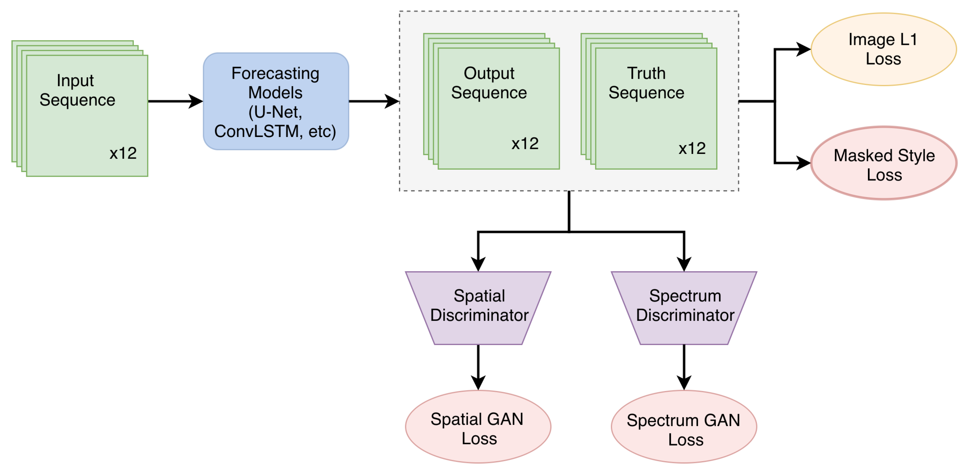
Both U-Net baseline and ConvLSTM baseline are trained with L1 loss, and the proposed losses are additionally applied in corresponding ablation studies. The batch size, learning rate, and maximum epochs were set to 16, $0.0002$, and 30, respectively. All experiments were optimized by AdamW using PyTorch and performed using 8 NVIDIA Tesla P100 (16 G) GPUs.

4.3. Baseline Models

We tested our methods with two baselines. The first is U-Net [16], which is a widely used backbone for CNN-based radar extrapolation methods. We followed the original paper [16] to build the network. It consists of a contracting path and an expansive path. The contracting path consists of repeated blocks of two $3\times 3$ convolutions, each followed by a rectified linear unit (ReLU) and a $2\times 2$ max pooling operation. We use four such blocks in the left path. The expansive path is symmetrical with the contracting path to recover the image size by using blocks of up-sampling, two $3\times 3$ convolutions, and a ReLU. Skip connections are adopted in each corresponding contracting and expansive block. Finally, feature maps from four expansive blocks are up-sampled to the original image size and fused by a $3\times 3$ convolution, and then sigmoid activation is used to obtain the final outputs.

The second baseline is ConvLSTM [12], which serves a test backbone of our methods for RNN-based radar extrapolation methods. The ConvLSTM consists of an encoding network and a forecasting network. Both networks are formed by stacking several convolutional LSTM layers, in which cell outputs and hidden states and gates are 3D tensors. Finally, all states in the forecasting network are fused by a $1\times 1$ convolution to generate the final prediction. We followed the original implementation of the network. More details can be found in [12].

4.4. Evaluation Metrics

We used two types of metric to evaluate model performance, i.e., forecast-specific metrics (CSI and BIAS) and perceptual-specific metrics (LPIPS and the proposed PSDS). Critical success index (CSI) and BIAS are commonly used metrics in forecast evaluation. In addition, since the main contribution of this paper is to tackle the blurring issue in radar extrapolation, we employed LPIPS and PSDS metrics for evaluating the sharpness of generated images and we will focus more on the performance of different methods on these two metrics.

As for CSI and BIAS, we first binarize the truth and prediction images at four thresholds, i.e., $[74,133,160,181]$. Then, we calculate true positive (TP, prediction = truth = 1), false positive (FP, prediction = 1, truth = 0), false negative (FN, prediction = 0, truth = 1), and true negative (TN, prediction = truth = 0). Finally, CSI and BIAS are computed as follows. As can be seen from the definitions, the range of CSI is $[0,1]$, and the higher the better; the range of BIAS is $[0,+\infty )$, and the closer it is to 1 the better.

$$\mathrm{CSI}=\frac{\mathrm{TP}}{\mathrm{TP}+\mathrm{FN}+\mathrm{FP}},\mathrm{BIAS}=\frac{\mathrm{TP}+\mathrm{FP}}{\mathrm{TP}+\mathrm{FN}}$$

(7)

LPIPS was proposed by Zhang et al. [22] to measure the perceptual similarity between two images, and has been shown to be more consistent with human judgment compared to traditional metrics (PSNR, SSIM [26], and FSIM [36]). The LPIPS metric can be obtained by computing the cosine distance of deep features in pre-trained networks, such as SqueezeNet [37], AlexNet [38], and VGGNet [39]. We use AlexNet in this paper. As the LPIPS measures deep feature distance, the lower it is the better.

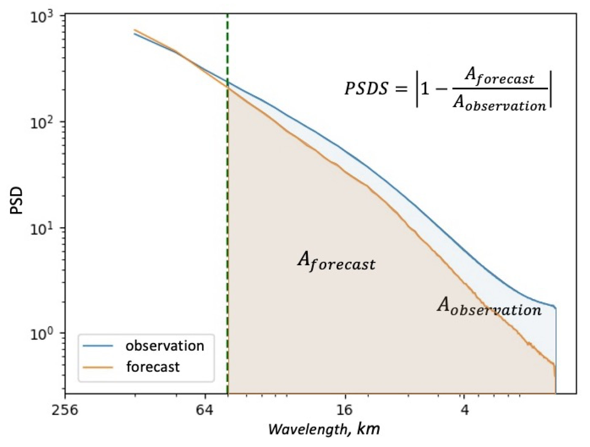
In addition, the proposed PSDS metric is also applied to evaluate the perceptual quality. In contrast with the LPIPS metric that measures the similarity of images in the feature space of pre-trained CNN models, the proposed PSDS measures their distances from the spectrum perspective (the lower the better). Therefore, these two metrics can be complementary to each other to better quantify the visual quality. One can refer to Section 3.3 for more details about the PSDS metric.

4.5. Experimental Results

In this subsection, we first describe ablation experiments with UNet and ConvLSTM baselines to investigate the effectiveness of each newly proposed component. Then, we discuss the influence of the weight of the masked style loss on both forecast performance and perceptual quality. All of the above experiments were conducted using the short-term prediction setting, in which 1 h future radar frames are predicted given 1 h past radar frames. Finally, we performed experiments using the long-term setting, in which we performed 2 h extrapolation given 1 h past radar sequences, to further verify our method’s generalizability for longer lead time.

Table 1. Ablation study for each proposed component on SEVIR dataset in terms of CSI, LPIPS, and PSDS. Experiments were conducted on UNet baseline with short-term prediction setting, in which 1 h future radar frames are predicted given 1 h past radar frames. ↑ denotes the higher the better, and ↓ denotes the lower the better.

Method	GAN		m. Style	CSI74 ↑	CSI133 ↑	CSI160 ↑	CSI181 ↑	LPIPS ↓	PSDS ↓
	Spatial	Spectrum
UNet baseline				0.5829	0.2551	0.1376	0.0900	0.3795	0.7245
Ours	✓			0.5637	0.2641	0.1496	0.1010	0.3325	0.5165
	✓	✓		0.5777	0.2816	0.1715	0.1292	0.3433	0.4308
	✓	✓	✓	0.5696	0.2780	0.1683	0.1276	0.2680	0.1586

and

Table 2. Ablation study for each proposed component on SEVIR dataset in terms of CSI, LPIPS, and PSDS. Experiments were conducted on ConvLSTM baseline with short-term prediction setting, in which 1 h future radar frames are predicted given 1 h past radar frames. ↑ denotes the higher the better, and ↓ denotes the lower the better.

Method	GAN		m. Style	CSI74 ↑	CSI133 ↑	CSI160 ↑	CSI181 ↑	LPIPS ↓	PSDS ↓
	Spatial	Spectrum
ConvLSTM baseline				0.5920	0.2582	0.1560	0.1104	0.4113	0.7782
Ours	✓			0.5828	0.2758	0.1754	0.1391	0.3743	0.3884
	✓	✓		0.5854	0.2814	0.1738	0.1281	0.3752	0.3373
	✓	✓	✓	0.5820	0.2767	0.1761	0.1395	0.2734	0.1566

show UNet-based and ConvLSTM-based ablation study results on each proposed component (spatial GAN, spectrum GAN, and masked style loss) on the SEVIR dataset, respectively. We compare CSI, LPIPS, and PSDS metrics in the same table so as to observe the model’s forecast performance and perceptual quality at the same time. In addition, BIAS for both UNet-based and ConvLSTM-based models is reported in

Table 3. UNet-based ablation experiments in terms of BIAS. Results are reported in the short-term setting (1 h extrapolation).

Method	GAN		m. Style	BIAS74	BIAS133	BIAS160	BIAS181
	Spatial	Spectrum
UNet baseline				0.9727	0.7457	0.3838	0.2854
Ours	✓			1.1388	1.3452	0.8028	0.5342
	✓	✓		1.0959	1.1697	0.7176	0.6022
	✓	✓	✓	1.1107	1.3172	0.9420	0.7365

and

Table 4. ConvLSTM-based ablation experiments in terms of BIAS. Results are reported in the short-term setting (1 h extrapolation).

Method	GAN		m. Style	BIAS74	BIAS133	BIAS160	BIAS181
	Spatial	Spectrum
ConvLSTM baseline				0.9575	0.6550	0.4403	0.3548
Ours	✓			0.9831	0.8818	0.6808	0.6832
	✓	✓		1.0274	0.9233	0.6351	0.5415
	✓	✓	✓	0.9946	0.9485	0.7222	0.6985

.

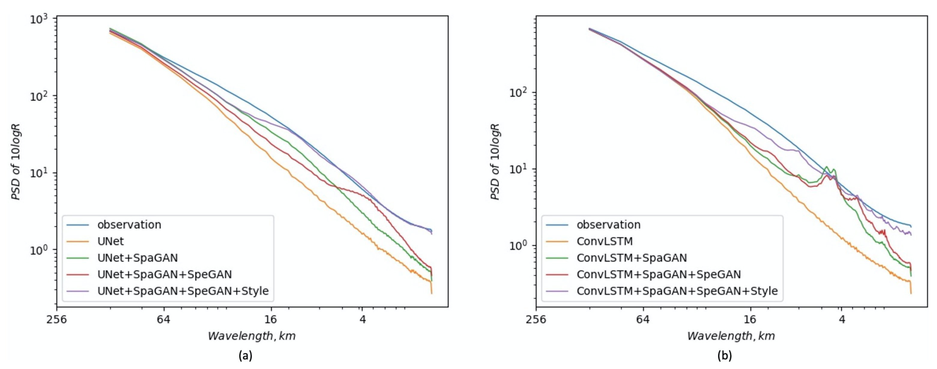
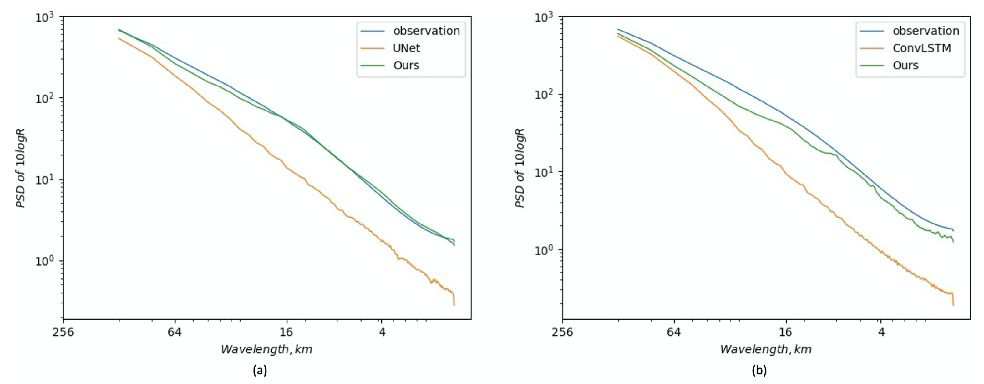
For UNet-based experiments, as shown in Table 1 (Row 1 and Row 2), the spatial GAN provides comparable performance to UNet baseline on CSI score. Specifically, some gains are observed for thresholds 133, 160, and 181, and a slight drop for threshold 174. Nevertheless, it achieves great improvements on LPIPS and PSDS scores (the lower the better), and the improvements can also be observed in the PSD curve. 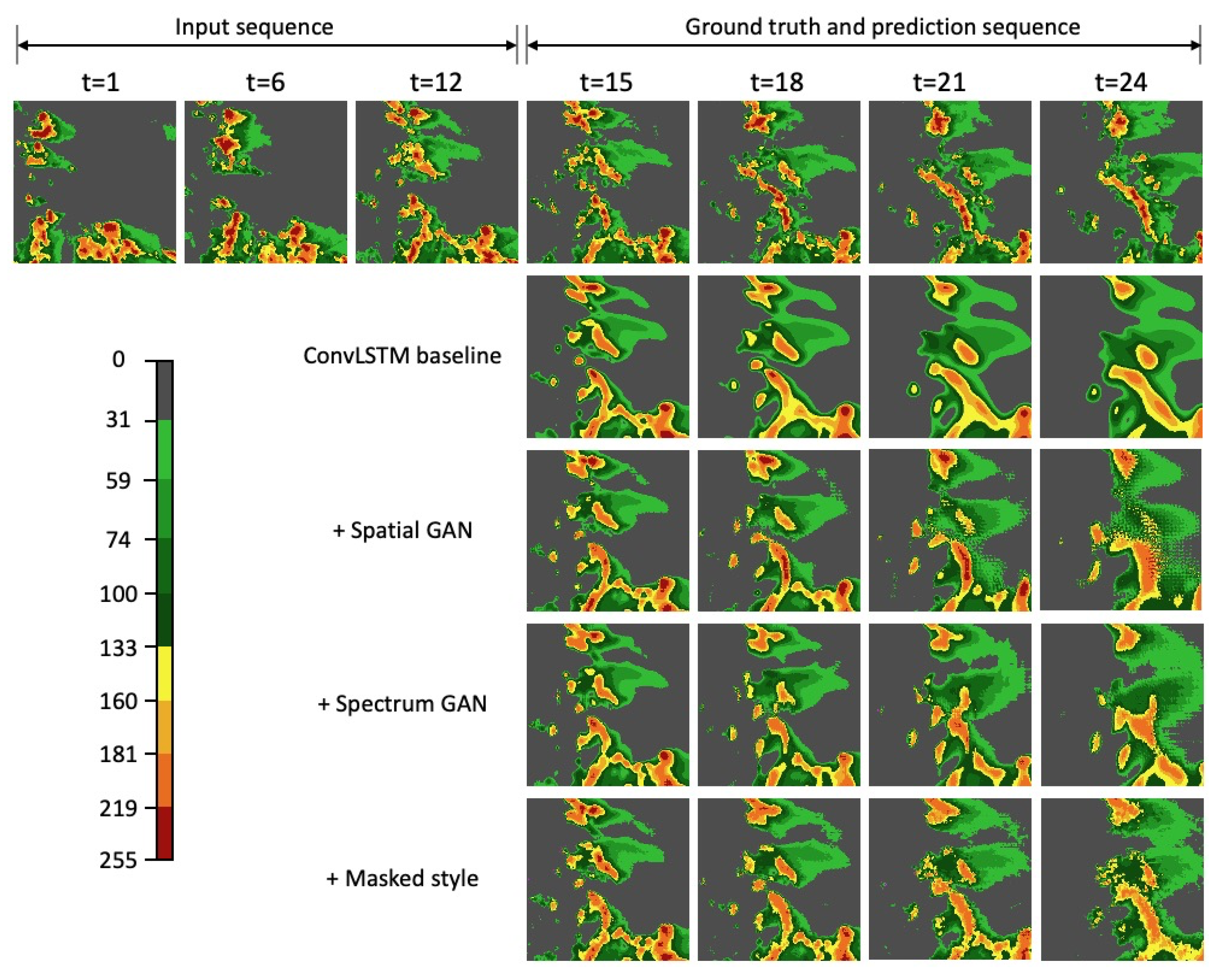As can be seen in Figure 4a, a substantial loss of power is apparent at wavelengths below 64 km for the UNet baseline. However, after adopting the spatial GAN, corresponding spectral power at small and medium scales is recovered significantly. 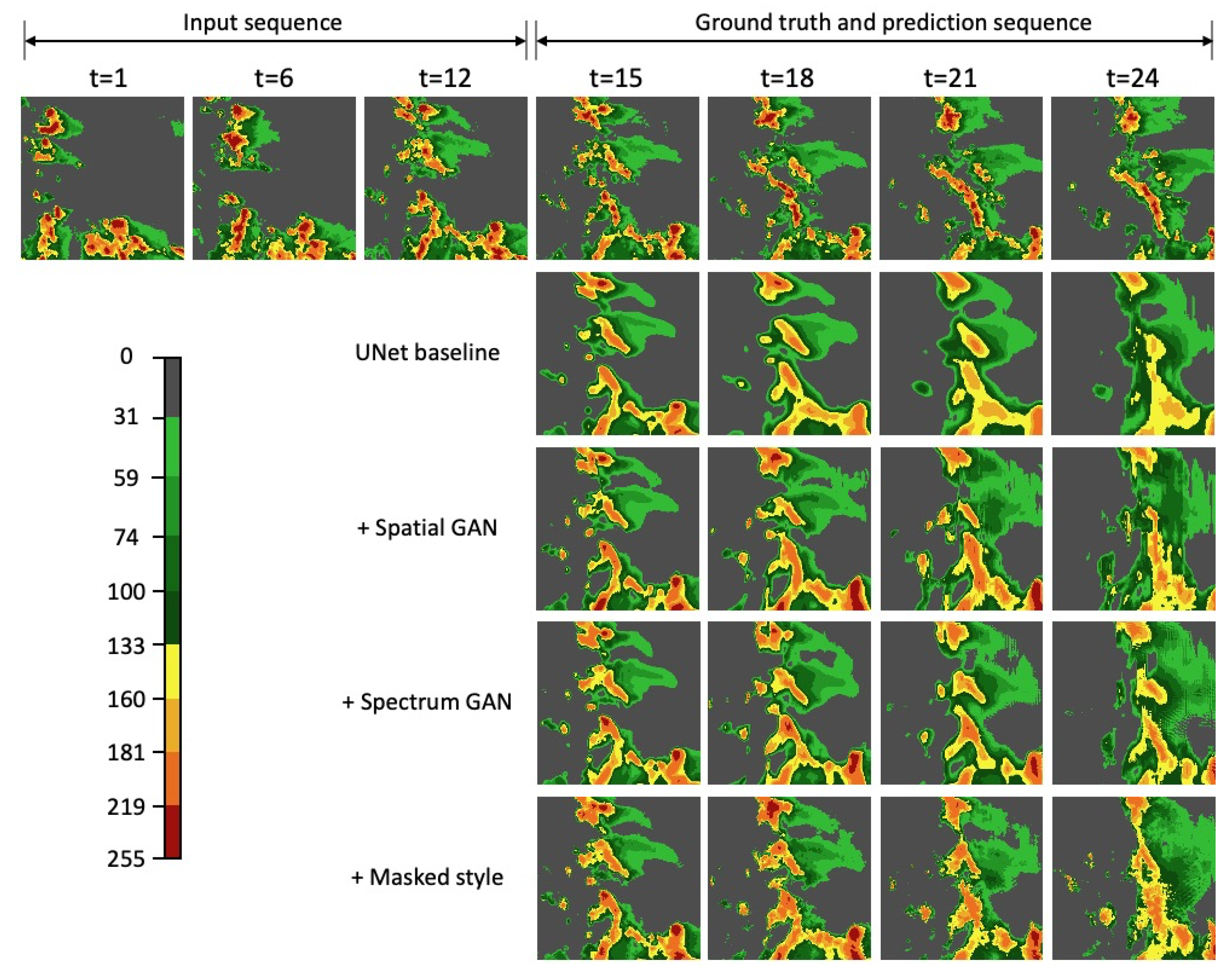We also visualize the extrapolation results in Figure 5. More details can be observed with the spatial GAN compared to the UNet baseline. Row 3 in Table 1 shows the results of further adding the spectrum GAN, which imposes additional supervision on the frequency domain. As shown in Table 1, the spectrum GAN provides remarkable improvements on CSI and PSDS scores. In the spectrum domain as shown in Figure 4a, the PSD curve of adding the spectrum GAN shows great power improvement at small scales (below 10 km) compared to the model without the spectrum GAN. Furthermore, in Figure 5, we can see that details become richer by further adding the spectrum GAN, which is especially obvious at a lead time of 1 h (t = 24 in Figure 5). It is also worth noting that the LPIPS score becomes slightly higher when adding the spectrum GAN, which does not agree with the PSDS score and visual impression. This phenomenon encourages joint analysis of different metrics, such as LPIPS, PSD, and the proposed PSDS, which are important for quantifying the visual performance of models comprehensively. Finally, as shown in Table 1 Row 3 and Row 4, further adding the masked style loss improves the perceptual quality significantly from $0.3433$ to $0.2680$ for LPIPS, and from $0.4308$ to $0.1586$ for PSDS, with only a slight drop in CSI scores. As shown in Figure 4a, the PSD curve of adding all proposed components achieves conspicuous improvements at scales below 16 km, and almost coincides with the observation curve. Qualitative results in Figure 5 show that we are able to achieve realistic and sharp extrapolations by further adding the masked style loss, and the prediction shows rich details even in a lead time of 1 h. In addition, Table 3 compares the BIAS between UNet baseline and the proposed method. As can be seen, the BIAS values at high thresholds [133, 160, 181] are far below 1 for UNet baseline, which means the model has difficulty in predicting high-intensity rainfall. However, by adding the proposed components, the BIAS values for high thresholds are improved, and the values for all thresholds fall in a reasonable range around 1. Overall, by leveraging the spatial GAN, spectrum GAN, and masked style loss, we can achieve not only significant improvements in visual quality (from 0.3795 to 0.2680 in terms of LPIPS, and from 0.7245 to 0.1586 in terms of PSDS), but also a remarkable performance boost at high VIL thresholds; specifically, $2.29\%$, $3.07\%$, and $3.76\%$ performance gains at thresholds 133, 160, and 181, respectively. These results demonstrate the effectiveness of the proposed methods for producing realistic radar extrapolation and improving performance at high rainfall regions.

For ConvLSTM-based experiments, similar results were obtained. As shown in Table 2 Row 1 and Row 4, our methods improve the visual performance significantly from $0.4113$ to $0.2734$ for LPIPS, and from $0.7782$ to $0.1566$ for PSDS. Moreover, CSI scores at high thresholds $[133,160,181]$ achieve improvements of $1.85\%$, $2.01\%$, and $2.91\%$, respectively, with only a small drop of $1.33\%$ at a low threshold of 74. Improvements in BIAS values also verify our method’s effectiveness in high rainfall region prediction, as shown in Table 4. Figure 4b shows the comparison of PSD curves. By adding all components, the PSD curve recovers most spectral power at scales below 16 km. In addition, we visualize some extrapolation results in Figure 6. As we can see, the predicted radar maps become sharper and achieve more detail with progressively adding the spatial GAN, spectrum GAN, and masked style loss.

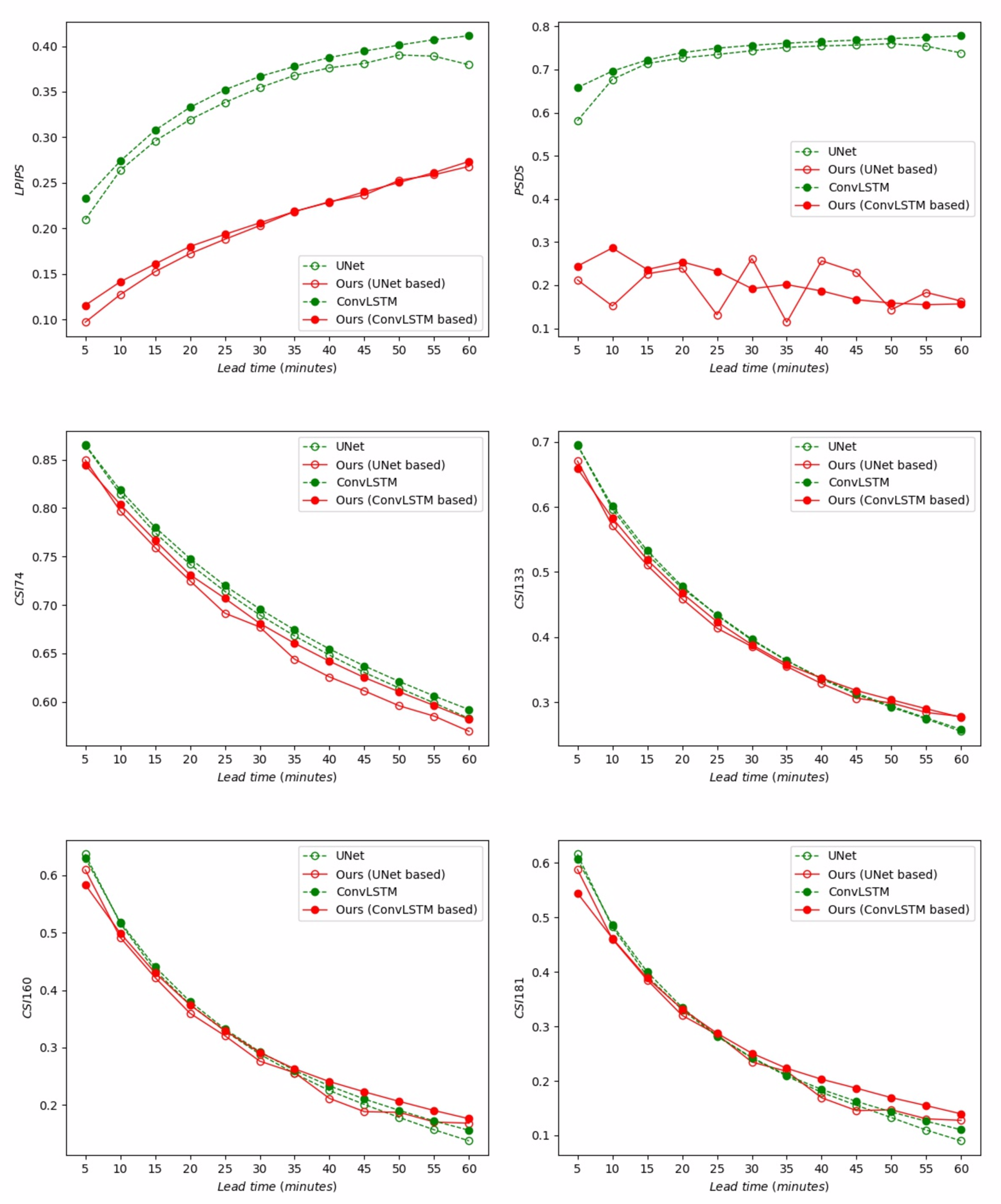
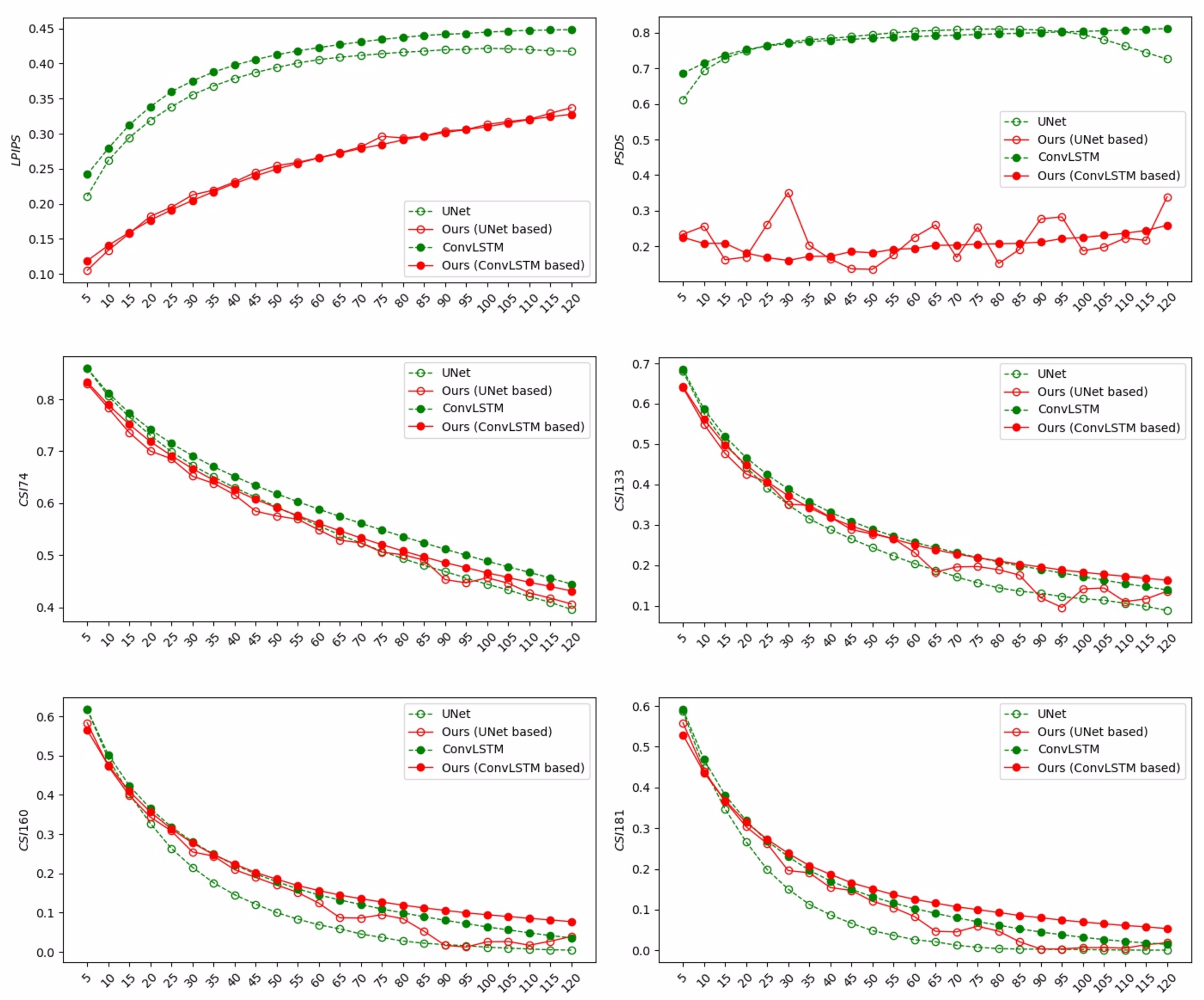
Moreover, we show the LPIPS, PSDS, and CSI curves against different lead times for UNet baseline, ConvLSTM baseline, and our methods in Figure 7. We can see a significant gap between LPIPS curves of baselines and our methods, and the performance of PSDS curves is similar, which justifies the effectiveness of the proposed methods for improving image sharpness and producing perceptually realistic nowcasting. As can be seen from the CSI curves, our methods show a slight drop for the low threshold 74, but begin to surpass the baselines at higher thresholds ($[133,160,181]$) and longer lead times (e.g., from 30 min to 60 min).

We then investigated the effect of the magnitude of the style weight ($\alpha$ in Equation (5)). As shown in

Table 5. The influence of the weight of the masked style loss on both forecast performance and perceptual quality. ↑ denotes the higher the better and ↓ denotes the lower the better.

Method	Weight	CSI74 ↑	CSI133 ↑	CSI160 ↑	CSI181 ↑	LPIPS ↓	PSDS ↓
UNet baseline	-	0.5829	0.2551	0.1376	0.0900	0.3795	0.7245
+masked style loss	5 × 10${}^5$	0.5425	0.2196	0.0905	0.0360	0.2615	0.1004
	1 × 10${}^5$	0.5710	0.2451	0.1091	0.0493	0.2513	0.2067
	5 × 10${}^4$	0.5680	0.2599	0.1427	0.0885	0.2529	0.1788
	1 × 10${}^4$	0.5801	0.2703	0.1337	0.0727	0.2622	0.3567

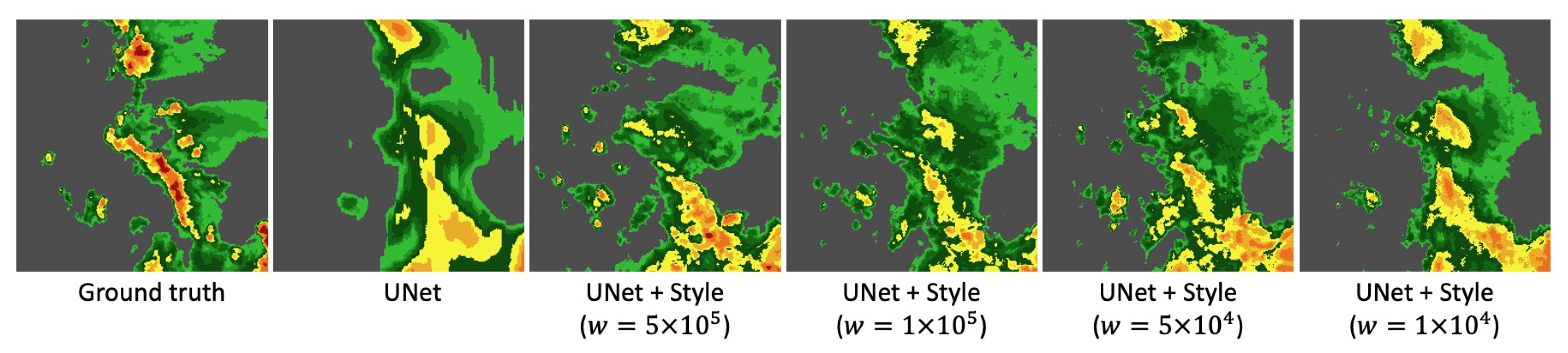
, we can see a tradeoff between forecast performance and perceptual quality when tuning the weight. For instance, with the decrease in the style weight from 5 × 10${}^5$ to 1 × 10${}^5$ in Table 5 Row 2 and Row 3, CSI scores gradually improve at all thresholds, but LPIPS and PSDS scores also increase, which means details are gradually lost. We set the weight to 1 × 10${}^4$ for all other experiments in this paper to obtain satisfactory perceptual quality without too much loss of forecast capability. We visualize 1 h extrapolation results of different style weights in Figure 8. We can see that the highest weight 5 × 10${}^5$ provides the most realistic extrapolation, and local details are getting lost with the decrease in the style weight. However, it is worth noting that, no matter how big the magnitude of the style weight is, applying the masked style loss can significantly improve the sharpness of prediction in comparison with baselines and produce realistic radar extrapolation.

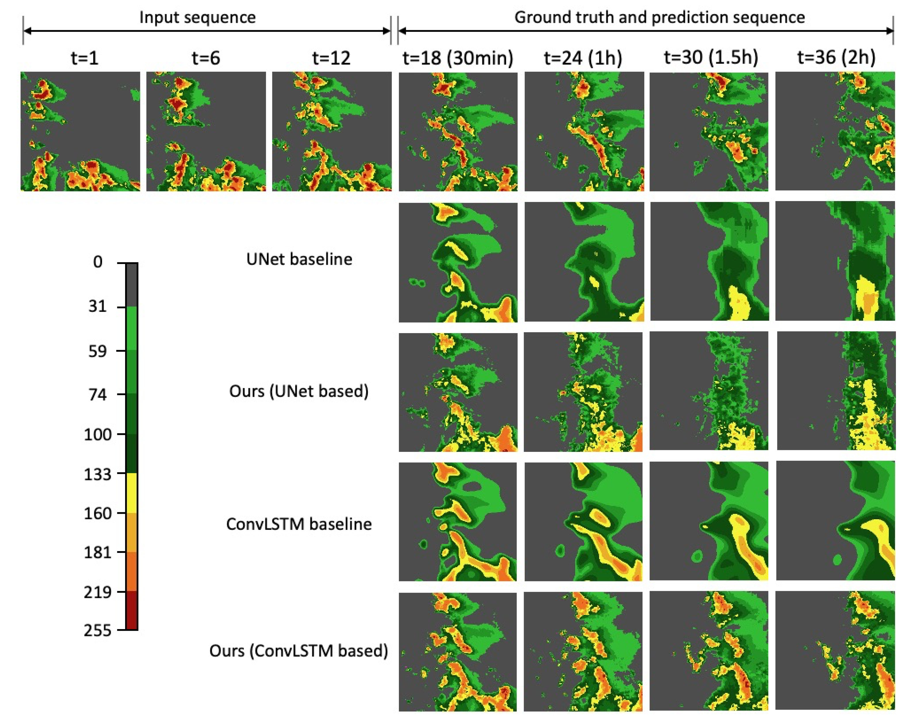
Finally, we performed comparison experiments in the long-term prediction setting to verify our method’s generalizability in extrapolating to longer lead times.

Table 6. Comparison experiments in terms of CSI, LPIPS, and PSDS metrics. Results are reported in the long-term prediction setting, in which we use past 1 h frames to predict future 2 h frames. ↑ denotes the higher the better, and ↓ denotes the lower the better.

Method	GAN		m. Style	CSI74 ↑	CSI133 ↑	CSI160 ↑	CSI181 ↑	LPIPS ↓	PSDS ↓
	Spatial	Spectrum
UNet baseline	✓	✓	✓	0.3961	0.0884	0.0045	0.0006	0.4173	0.7258
Ours				0.4063	0.1357	0.0394	0.0187	0.3371	0.3393
ConvLSTM baseline	✓	✓	✓	0.4449	0.1391	0.0356	0.0147	0.4483	0.8115
Ours				0.4315	0.1632	0.0772	0.0533	0.3276	0.2590

and

Table 7. Comparison experiments in term of BIAS. Results are reported in the long-term setting (2 h extrapolation).

Method	GAN		m. Style	BIAS74	BIAS133	BIAS160	BIAS181
	Spatial	Spectrum
UNet baseline	✓	✓	✓	0.8175	0.3088	0.0255	0.0066
Ours				1.3216	1.2457	0.6640	0.5155
ConvLSTM baseline	✓	✓	✓	0.8349	0.4365	0.1287	0.0690
Ours				0.9200	0.8154	0.5668	0.5237

show the results based on UNet and ConvLSTM baselines in terms of CSI, BIAS, LPIPS, and PSDS metrics. As we can see, our methods are able to improve perceptual scores (LPIPS and PSDS) significantly. In addition, it is worth noting that our methods provide remarkable performance gains in high rainfall prediction, as can be seen from CSI and BIAS results in Table 6 and Table 7. The BIAS values at thresholds $[133,160,181]$ are far below 1, and values at $[160,181]$ are almost close to 0, which means the baselines are unable to predict high rainfall. However, by adding the proposed components, the CSI and BIAS scores obtain significant improvements. The phenomenon can also be observed in Figure 9 and Figure 10. ConvLSTM-based models outperform UNet-based models in 2 h extrapolation.

Again, we also show the nowcasting performance against different lead times from 5 to 120 min in terms of LPIPS, PSDS, and CSI scores in Figure 11. For LPIPS and PSDS, the trends are similar. There are apparent gaps between baselines (both UNet and ConvLSTM) and our methods. In addition, we observe that the PSDS curve of our methods (UNet-based) is not smooth, which means the predicted sequence may have poor time consistency, i.e., flicker between neighboring frames. This issue can be solved by temporal consistency loss [40,41,42], or temporal discriminator [30], which is outside the scope of this work. For the CSI curve, we can see that our methods decrease the CSI score at a low threshold, i.e., 74. However, the proposed methods improve the performance at a higher intensity (i.e., $[133,160,181]$) and longer lead time (e.g., from 30 min to 120 min). It is worth noting that as the lead time increases, the gap between our methods and baselines becomes more and more significant, and it is more obvious at higher thresholds (e.g., 160 and 181). The above results demonstrate that the proposed methods are able to improve the image sharpness of different baseline models significantly as well as improving forecasting performance at high rainfall regions, even in a long lead time up to 2 h.

5. Discussion

In this paper, we proposed effective strategies, a spatial GAN, a spectrum GAN, and a masked style loss, to tackle the blurring problem in prior deep-learning-based radar extrapolation models, including CNN-based and LSTM-based models. Here, we provide some discussions on the generalization of our methods, time consistency problem, and perceptual evaluation metrics.

We first analyze the generalization of our methods. We performed the same experiments with U-Net and ConvLSTM baselines, which are both typical models used in CNN-based and LSTM-based radar nowcasting methods. Our methods significantly improve the visual quality of the extrapolations on both baselines. We then claimed that our methods can be easily applied to other deep-learning-based radar forecasting models to achieve realistic extrapolation results. In addition, experiments in short-term (1 h) and long-term (2 h) prediction settings have shown that our methods can generalize well to longer lead times, and qualitative results have shown that our methods can generate sharp and realistic images even in the lead time of 2 h and maybe longer, which can be verified in future research. We can say that our methods take a step further towards an operational nowcasting system to assist the forecaster in weather forecasting by providing detailed and realistic prediction results.

Second, we discuss the time consistency problem. We observed the flickering phenomenon in the predicted sequence of the UNet-based model—the time consistency of its output sequence is poor. As mentioned in experiments, this issue can also be observed in the PSDS curve. The problem comes to light when the extrapolated results become very detailed and are thus sensitive to subtle differences between consecutive frames. However, this is not so obvious in the ConvLSTM-based model. The reason may be that UNet has a poor capability of modeling relationships in long sequences along the time dimension, while ConvLSTM predicts the next frames based on the last generated ones iteratively and has better time consistency even if the extrapolations become very detailed. However, the time consistency can be improved using temporal consistency loss or temporal discriminator, etc., which can be studied in future work.

Finally, we discuss the perceptual evaluation metrics. Evaluation metrics for measuring visual quality are important for the development of realistic radar echo extrapolation methods. Traditional metrics, such as SSIM and PSNR, have poor consistency with human judgment. The proposed PSDS in this paper, as well as the recently proposed LPIPS, has higher agreement with human assessment. However, in our experiments, we found that the two metrics sometimes disagree with each other. This may be because LPIPS and PSDS are calculated from different domains (feature domain and frequency domain, respectively). Therefore, we recommend future researchers to use metrics from both spatial and frequency domains to evaluate the perceptual quality objectively and comprehensively. Better perceptual evaluation metrics that are specific to radar extrapolation tasks could be a meaningful research direction.

6. Conclusions

This paper has mainly focused on tackling the notorious blurring issue in existing deep-learning-based radar echo nowcasting models.

• First, we proposed a spatial GAN and a spectrum GAN to improve image fidelity. Spatial and spectrum GANs are able to penalize the differences between generated and real images in spatial and spectral domains, respectively.
• Second, we proposed a masked style loss to transfer the detailed texture of ground truth sequences to predicted sequences. Especially, a foreground mask was used to avoid the background noise being transferred to the output.
• Third, we designed the power spectral density score (PSDS) to measure the perceptual quality of predicted imagery from the spectrum perspective. PSDS can be used as a complement to other visual quality evaluation metrics (e.g., LPIPS) so as to obtain a comprehensive and objective measurement for image similarity.
• Finally, comprehensive experiments on the SEVIR dataset verified the effectiveness of the proposed methods for improving image details significantly (as shown in Figure 5, Figure 6 and Figure 10). Moreover, our method can be readily applied to any spatiotemporal forecasting models to acquire realistic predictions.

References

1. Wilson, J.W.; Crook, N.A.; Mueller, C.K.; Sun, J.; Dixon, M. Nowcasting thunderstorms: A status report. Bull. Am. Meteorol. Soc. 1998, 79, 2079–2100. [Google Scholar] [CrossRef]
2. Sun, J.; Xue, M.; Wilson, J.W.; Zawadzki, I.; Ballard, S.P.; Onvlee-Hooimeyer, J.; Joe, P.; Barker, D.M.; Li, P.W.; Golding, B.; et al. Use of NWP for nowcasting convective precipitation: Recent progress and challenges. Bull. Am. Meteorol. Soc. 2014, 95, 409–426. [Google Scholar] [CrossRef] [Green Version]
3. Dixon, M.; Wiener, G. TITAN: Thunderstorm identification, tracking, analysis, and nowcasting—A radar-based methodology. J. Atmos. Ocean. Technol. 1993, 10, 785–797. [Google Scholar] [CrossRef]
4. Li, L.; Schmid, W.; Joss, J. Nowcasting of motion and growth of precipitation with radar over a complex orography. J. Appl. Meteorol. Climatol. 1995, 34, 1286–1300. [Google Scholar] [CrossRef] [Green Version]
5. del Moral, A.; Rigo, T.; Llasat, M.C. A radar-based centroid tracking algorithm for severe weather surveillance: Identifying split/merge processes in convective systems. Atmos. Res. 2018, 213, 110–120. [Google Scholar] [CrossRef]
6. Lucas, B.D.; Kanade, T. An iterative image registration technique with an application to stereo vision. In Proceedings of the 7th International Joint Conference on Artificial Intelligence, Vancouver, BC, Canada, 24–28 August 1981. [Google Scholar]
7. Ayzel, G.; Scheffer, T.; Heistermann, M. RainNet v1. 0: A convolutional neural network for radar-based precipitation nowcasting. Geosci. Model Dev. 2020, 13, 2631–2644. [Google Scholar] [CrossRef]
8. Reichstein, M.; Camps-Valls, G.; Stevens, B.; Jung, M.; Denzler, J.; Carvalhais, N. Deep learning and process understanding for data-driven Earth system science. Nature 2019, 566, 195–204. [Google Scholar] [CrossRef]
9. Ayhan, B.; Kwan, C.; Budavari, B.; Kwan, L.; Lu, Y.; Perez, D.; Li, J.; Skarlatos, D.; Vlachos, M. Vegetation detection using deep learning and conventional methods. Remote Sens. 2020, 12, 2502. [Google Scholar] [CrossRef]
10. Xu, Y.; Wu, L.; Xie, Z.; Chen, Z. Building extraction in very high resolution remote sensing imagery using deep learning and guided filters. Remote Sens. 2018, 10, 144. [Google Scholar] [CrossRef] [Green Version]
11. Sønderby, C.K.; Espeholt, L.; Heek, J.; Dehghani, M.; Oliver, A.; Salimans, T.; Agrawal, S.; Hickey, J.; Kalchbrenner, N. Metnet: A neural weather model for precipitation forecasting. arXiv 2020, arXiv:2003.12140. [Google Scholar]
12. Xingjian, S.H.I.; Chen, Z.; Wang, H. Convolutional LSTM network: A machine learning approach for precipitation nowcasting. In Proceedings of the Advances in Neural Information Processing Systems, Montreal, QC, Canada, 7–12 December 2015; pp. 802–810. [Google Scholar]
13. Shi, X.; Gao, Z.; Lausen, L.; Wang, H.; Yeung, D.Y.; Wong, W.K.; Woo, W.C. Deep learning for precipitation nowcasting: A benchmark and a new model. arXiv 2017, arXiv:1706.03458. [Google Scholar]
14. Wang, Y.; Long, M.; Wang, J.; Gao, Z.; Yu, P.S. Predrnn: Recurrent neural networks for predictive learning using spatiotemporal lstms. In Proceedings of the 31st International Conference on Neural Information Processing Systems, Long Beach, CA, USA, 4 December 2017; pp. 879–888. [Google Scholar]
15. Wang, Y.; Zhang, J.; Zhu, H.; Long, M.; Wang, J.; Yu, P.S. Memory in memory: A predictive neural network for learning higher-order non-stationarity from spatiotemporal dynamics. In Proceedings of the IEEE/CVF Conference on Computer Vision and Pattern Recognition, Long Beach, CA, USA, 15–20 June 2019; pp. 9154–9162. [Google Scholar]
16. Ronneberger, O.; Fischer, P.; Brox, T. U-net: Convolutional networks for biomedical image segmentation. In Proceedings of the International Conference on Medical Image Computing and Computer-Assisted Intervention, Munich, Germany, 5–9 October 2015; pp. 234–241. [Google Scholar]
17. Weyn, J.A.; Durran, D.R.; Caruana, R. Improving data-driven global weather prediction using deep convolutional neural networks on a cubed sphere. J. Adv. Model. Earth Syst. 2020, 2, e2020MS002109. [Google Scholar] [CrossRef]
18. Zhou, K.; Zheng, Y.; Dong, W.; Wang, T. A deep learning network for cloud-to-ground lightning nowcasting with multisource data. J. Atmos. Ocean. Technol. 2020, 37, 927–942. [Google Scholar] [CrossRef]
19. Veillette, M.; Samsi, S.; Mattioli, C. SEVIR: A Storm Event Imagery Dataset for Deep Learning Applications in Radar and Satellite Meteorology. In Proceedings of the 34th Conference on Neural Information Processing Systems (NeurIPS 2020), Vancouver, BC, Canada, 6–12 December 2020; Volume 33. [Google Scholar]
20. Tran, Q.K.; Song, S. Computer vision in precipitation nowcasting: Applying image quality assessment metrics for training deep neural networks. Atmosphere 2019, 10, 244. [Google Scholar] [CrossRef] [Green Version]
21. Mathieu, M.; Couprie, C.; LeCun, Y. Deep multi-scale video prediction beyond mean square error. arXiv 2015, arXiv:1511.05440. [Google Scholar]
22. Talebi, H.; Milanfar, P. Learned perceptual image enhancement. In Proceedings of the 2018 IEEE international conference on computational photography (ICCP), Pittsburgh, PA, USA, 4–6 May 2018; pp. 1–13. [Google Scholar]
23. Wu, H.; Yao, Z.; Wang, J.; Long, M. MotionRNN: A flexible model for video prediction with spacetime-varying motions. In Proceedings of the IEEE/CVF Conference on Computer Vision and Pattern Recognition, Nashville, TN, USA, 19–25 June 2021; pp. 15435–15444. [Google Scholar]
24. Pan, X.; Lu, Y.; Zhao, K.; Huang, H.; Wang, M.; Chen, H. Improving Nowcasting of Convective Development by Incorporating Polarimetric Radar Variables into a Deep Learning Model. Geophys. Res. Lett. 2021, 48, e2021GL095302. [Google Scholar] [CrossRef]
25. Yin, J.; Gao, Z.; Han, W. Application of a Radar Echo Extrapolation-Based Deep Learning Method in Strong Convection Nowcasting. Earth Space Sci. 2021, 8, e2020EA001621. [Google Scholar] [CrossRef]
26. Wang, Z.; Bovik, A.C.; Sheikh, H.R.; Simoncelli, E.P. Image quality assessment: From error visibility to structural similarity. IEEE Trans. Image Process. 2004, 13, 600–612. [Google Scholar] [CrossRef] [Green Version]
27. Wang, Z.; Simoncelli, E.P.; Bovik, A.C. Multiscale structural similarity for image quality assessment. In Proceedings of the Thrity-Seventh Asilomar Conference on Signals, Systems & Computers, Pacific Grove, CA, USA, 9–12 November 2003; IEEE: Piscataway, NJ, USA, 2003; Volume 2, pp. 1398–1402. [Google Scholar]
28. Jing, J.; Li, Q.; Peng, X. MLC-LSTM: Exploiting the spatiotemporal correlation between multi-level weather radar echoes for echo sequence extrapolation. Sensors 2019, 19, 3988. [Google Scholar] [CrossRef] [Green Version]
29. Tian, L.; Li, X.; Ye, Y. A generative adversarial gated recurrent unit model for precipitation nowcasting. IEEE Geosci. Remote Sens. Lett. 2019, 17, 601–605. [Google Scholar] [CrossRef]
30. Ravuri, S.; Lenc, K.; Willson, M. Skillful Precipitation Nowcasting using Deep Generative Models of Radar. arXiv 2021, arXiv:2104.00954. [Google Scholar]
31. Zhang, R.; Isola, P.; Efros, A.A.; Shechtman, E.; Wang, O. The unreasonable effectiveness of deep features as a perceptual metric. In Proceedings of the IEEE Conference on Computer Vision and Pattern Recognition, Salt Lake City, UT, USA, 18–22 June 2018; pp. 586–595. [Google Scholar]
32. Chen, Y.; Li, G.; Jin, C. SSD-GAN: Measuring the Realness in the Spatial and Spectral Domains. arXiv 2020, arXiv:2012.05535. [Google Scholar]
33. Gatys, L.A.; Ecker, A.S.; Bethge, M. Image style transfer using convolutional neural networks. In Proceedings of the IEEE Conference on Computer Vision and Pattern Recognition, Las Vegas, NV, USA, 27–30 June 2016; pp. 2414–2423. [Google Scholar]
34. Johnson, J.; Alahi, A.; Fei-Fei, L. Perceptual losses for real-time style transfer and super-resolution. In European Conference on Computer Vision; Springer: Berlin/Heidelberg, Germany, 2016; pp. 694–711. [Google Scholar]
35. Welch, P. The use of fast Fourier transform for the estimation of power spectra: A method based on time averaging over short, modified periodograms. IEEE Trans. Audio Electroacoust. 1967, 15, 70–73. [Google Scholar] [CrossRef] [Green Version]
36. Zhang, L.; Zhang, L.; Mou, X. FSIM: A feature similarity index for image quality assessment. IEEE Trans. Image Process. 2011, 20, 2378–2386. [Google Scholar] [CrossRef] [PubMed] [Green Version]
37. Iandola, F.N.; Han, S.; Moskewicz, M.W.; Ashraf, K.; Dally, W.J.; Keutzer, K. SqueezeNet: AlexNet-level accuracy with 50x fewer parameters and< 0.5 MB model size. arXiv 2016, arXiv:1602.07360. [Google Scholar]
38. Krizhevsky, A.; Sutskever, I.; Hinton, G.E. Imagenet classification with deep convolutional neural networks. Adv. Neural Inf. Process. Syst. 2012, 25, 1097–1105. [Google Scholar] [CrossRef]
39. Simonyan, K.; Zisserman, A. Very deep convolutional networks for large-scale image recognition. arXiv 2014, arXiv:1409.1556. [Google Scholar]
40. Gupta, A.; Johnson, J.; Alahi, A.; Fei-Fei, L. Characterizing and improving stability in neural style transfer. In Proceedings of the IEEE International Conference on Computer Vision, Venice, Italy, 22–29 October 2017; pp. 4067–4076. [Google Scholar]
41. Lai, W.S.; Huang, J.B.; Wang, O.; Shechtman, E.; Yumer, E.; Yang, M.H. Learning blind video temporal consistency. In Proceedings of the European Conference on Computer Vision (ECCV), Munich, Germany, 8–14 September 2018; pp. 170–185. [Google Scholar]
42. Mallya, A.; Wang, T.C.; Sapra, K.; Liu, M.Y. World-consistent video-to-video synthesis. In Proceedings of the Computer Vision—ECCV 2020: 16th European Conference, Glasgow, UK, 23–28 August 2020; pp. 359–378. [Google Scholar]
Figure 1. The main pipeline and schematic illustration of our approach.
Remotesensing 14 00024 g001
Figure 2. Illustration of spatial discriminator (a) and spectral discriminator (b).
Remotesensing 14 00024 g002
Figure 3. Illustration of PSDS metric.
Remotesensing 14 00024 g003
Figure 4. Comparison of each proposed component in terms of PSD curve. Results are reported in the short-term setting (1 h extrapolation). (a) UNet-based models; (b) ConvLSTM-based models.
Remotesensing 14 00024 g004
Figure 5. Qualitative comparison for each proposed component (UNet-based). Experiments were performed in the short-time prediction setting (1 h extrapolation).
Remotesensing 14 00024 g005
Figure 6. Qualitative comparison for each proposed component (ConvLSTM-based). Experiments were performed in the short-time prediction setting (1 h extrapolation).
Remotesensing 14 00024 g006
Figure 7. Nowcast performance against different lead times for UNet, ConvLSTM, and our methods in terms of LPIPS, PSDS, and CSI scores. Experiments were performed in the short-time prediction setting (1 h extrapolation).
Remotesensing 14 00024 g007
Figure 8. Qualitative comparison of different style weights.
Remotesensing 14 00024 g008
Figure 9. Comparison of each proposed component in terms of PSD curve. (a) UNet-based models; (b) ConvLSTM-based models.
Remotesensing 14 00024 g009
Figure 10. Qualitative comparison for each proposed component (UNet-based). Experiments were performed in the short-time prediction setting (1 h extrapolation).
Remotesensing 14 00024 g010
Figure 11. Nowcasting performance against different lead times for UNet, ConvLSTM, and our methods in terms of LPIPS, PSDS, and CSI scores. Experiments were performed in the long-time prediction setting (2 h extrapolation).
Remotesensing 14 00024 g011