Abstract
It is difficult to detect ports in polarimetric SAR images due to the complicated components, morphology, and coastal environment. This paper proposes an unsupervised port detection method by extracting the water of the port based on three-component decomposition and multi-scale thresholding segmentation. Firstly, the polarimetric characteristics of the port water are analyzed using modified three-component decomposition. Secondly, the volume scattering power and the power ratio of the double-bounce scattering power to the volume scattering power (PRDV) are used to extract the port water. Water and land are first separated by a global thresholding segmentation of the volume scattering power, in which the sampling region used for the threshold calculation is automatically selected by a proposed homogeneity measure. The interference water regions in the ports are then separated from the water by segmenting the PRDV using the multi-scale thresholding segmentation method. The regions of interest (ROIs) of the ports are then extracted by determining the connected interference water regions with a large area. Finally, ports are recognized by examining the area ratio of strong scattering pixels to the land in the extracted ROIs. Seven single quad-polarization SAR images acquired by RADARSAT-2 covering the coasts of Dalian, Zhanjiang, Fujian, Tianjin, Lingshui, and Boao in China and Berkeley in America are used to test the proposed method. The experimental results show that all ports are correctly and quickly detected. The false alarm rates are zero, the intersection of union section (IoU) indexes between the detected port and the ground truth can reach 75%, and the average processing time can be less than 100 s.
1. Introduction
Ports are important stationary facilities for cargo distribution and ships to berth on the coast. The automatic detection of ports in remote sensing images is of great significance for coastal terrains monitoring, marine navigation, terrain registration, port ship detection, port security, and port-disaster preparedness [1,2,3]. As shown in Figure 1, a port is located at the junction of the land and sea, which is composed of jetties, breakwaters, several man-made buildings, berthed ships, and port water. Due to the protruding jetties and breakwaters, the geometric structure of the port is so distinct that its detection is simple. However, although some ports can be easily detected by extracting the specific geometric features, it is difficult to correctly detect all ports due to the variety of shapes, the noise and strong interference, and the sophisticated coastal terrains background [2]. There will be many false alarms generated by the natural raised terrain using the geometric method.
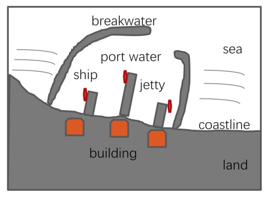
Figure 1.
Structure diagram of a port, where the boxes drawn in orange denote buildings, and the red boxes denote ships.
Because the geometric feature of ports is salient, almost all existing port and small harbor detection methods are based on the extraction of the specific geometric features [1,2,3,4,5,6,7,8,9]. Usually, the geometric-based methods mainly include three steps: sea-land segmentation, geometric feature extraction, and feature measure and classification. The sea and land are segmented to extract the coastline using an edge-based or region-based segmentation method first [10,11,12,13]. The geometric features of corners or lines are then extracted from the coastline using angular detection [14] or polygon fitting of the digital curve [15]. Sometimes, the geometric features of protruding jetties are extracted by a jetty scanning method [7]. Finally, ports are detected by measuring the parallel and broken lines [2,4], the concavity and convexity, or the closure of the contours [6,7,8].
In the step of the sea–land segmentation, the existing methods usually take a two-step strategy to detect the coastline from coarse to fine. A coarse result is globally extracted by a region-based segmentation or an edge detection method first. A coarse result is then locally refined by an edge-based active contour model or Markov field segmentation. Liu et al. [10] extracted coarse sea–land segmentation results using a region-based level set method and refined coarse results using an edge-based active contour model. Schmitt et al. [11] constructed a multi-scale image space and segmented water and land from coarse to fine using the K-medians classification method in different scale-spaces. Liu et al. [12] segmented water and land from coarse to fine using a narrow-band level set method in different scale-spaces. Modava et al. [13] extracted rough land-sea segmentation by utilizing a texture-based segmentation using local spectral histogram and refined the coarse result using region-based level set segmentation. The existing methods are all intensity-based methods. Accurate sea–land segmentation results can be obtained when the difference of the intensity or the coherent matrix between the sea and land are distinct. When the coastal environment is harsh, the intensities of some water regions in a high sea state are higher than the intensities of the land regions, and the intensities of mud and sand flats in intertidal zones are lower than the intensities of the calm sea regions. Wrong segmentation will then occur in both sea and land regions. To avoid the wrong segmentation caused by the intensity intersection of different regions, Wang et al. [16] proposed a classification scheme of mud and sand flats on intertidal flats using different polarimetric decomposition components. Ferrentino et al. [17] proposed a coastline extraction scheme in harsh coastal environments using a global constant false alarm rate (CFAR) thresholding segmentation of a normalized cross-section in different polarimetric channels. However, it is still difficult to segment the land and water along ports using the existing polarimetric methods since the port water regions are interfered with by surrounding strong scattering buildings and ships.
Based on the accurate sea–land segmentation, the geometric features of the contour of ports can then be extracted and recognized. From the point of view that the feature points of the outline of the port area are denser than those of non-port areas, Liu et al. [2] proposed a harbor detection method based on feature point merging. Starting from the assumption that the two sides of jetties and breakwaters are parallel, Liu et al. [3] proposed a harbor detection method based on the characteristics of parallel curves. Starting from the assumption that the overall structural characteristics of the port contour are in order, Li et al. [4] detected the port by extracting corners on the contour using wavelet transform and described the corners using chain code descriptors. He et al. [5] detected a harbor by a combination of edge detection and scale-invariant feature transform keypoint extraction. According to the assumption that the contours of jetties were concave and convex, Chen et al. [6] first proposed a method based on jetty scanning and merging. Zhao et al. [7] improved the scanning method from two directions to four directions. Liu et al. [8] extended the method from four directions to multiple directions. However, the problem of the above geometric-feature-based methods is that the geometric features of ports are unstable and blur in SAR images due to the strong coherent speckle, the variety of port morphology, and the berthed ships on the port. Accurate coastline detection and sophisticated feature extraction methods are needed to detect and measure blurry geometric features. This directly leads to a decrease in accuracy and an increase in computational time. When the sea condition is rough and the interference is strong, wrong segmentation and incorrect feature extraction will make the port undetectable. When the coastal outline is complex, the natural protruding terrain along the coast will form false alarms.
In recent years, deep learning neural network methods, including the Region-based Convolutional Neural Network (R-CNN) [18], the Fast/Faster R-CNN [19], and the Mask R-CNN [20], are widely used in all kinds of object detection. However, it is difficult to collect sufficient training samples to perform port detection in SAR images because of the varied morphology of ports and the strong coherent speckle.
Compared with port detection in optical remote sensing images, ports in synthetic aperture radar (SAR) images not only have salient geometric features but also have a significant scattering intensity distribution feature formed by the surrounding buildings and ships. The extraction of a strong scattering region can provide effective information for port detection in SAR images. When the candidate regions of interest (ROIs) have been extracted by a geometric method, false alarms formed by naturally raised terrain can be eliminated by calculating the area ratio of the strong scattering region in a port. Liu et al. [8] extracted a strong scattering region using a three-region level set segmentation method to eliminate the false alarms extracted by jetty scanning. In polarimetric SAR images, the scattering components of ports are complex due to the multiple scattering between buildings and the ground terrain. Thus, port detection in polarimetric SAR images can also use the specific polarimetric scattering components of port buildings and water regions. To eliminate the double-bounce scattering interference generated by a strong scatterer, Liu et al. [2] extracted the volume scattering component using Freeman three-component decomposition [21] or four-component decomposition [22] to segment the sea and land. Except for the volume scattering component, polarimetric entropy [23], polarimetric cross-entropy [24], the generalized optimization of polarimetric contrast enhancement (GOPCE) [25], the similarity parameter [26], the degree of polarization [27], etc. are all useful polarimetric parameters to represent buildings on a port. However, since the scattering characteristics of buildings in a port are almost the same as those of buildings outside the port, the above parameters are difficult to directly use for port detection.
Except for the geometric features of protruding jetties and breakwaters and the specific polarimetric scattering features of buildings on the port, port water is also an important and special component of a port in polarimetric SAR images. Because of the scattering interference of man-made buildings and ships in ports, the port water appears to be different from calm water regions in the Pauli pseudocolor image of polarimetric SAR. Statistics results show that the polarimetric parameters of port water, such as double-bounce scattering power and polarimetric entropy, are all different from those of calm water [2]. Thus, this paper proposes an unsupervised port detection method by extracting port water using a proposed polarimetric parameter based on three-component decomposition in polarimetric SAR images. The main contributions can be summarized as follows:
1. Unlike traditional methods based on the geometric features extraction of port contours or deep learning methods based on the data representation of port regions, we propose a port detection method based on port water extraction.
2. A polarimetric parameter of the power ratio of the double-bounce scattering power to the volume scattering power is proposed to extract port water based on the three-component decomposition of polarimetric SAR images.
3. A simple global CFAR multi-scale thresholding segmentation method is proposed to segment port water regions and other regions.
The rest of this paper is organized as follows. In Section 2, the three-component decomposition and the modified three-component decomposition are described briefly. In Section 3, the proposed method is introduced in detail. Experimental results will be shown and discussed in Section 4. The conclusion is given in Section 5.
2. Three-Component Decomposition
According to Freeman–Durden three-component decomposition [21], for a multi-look polarimetric SAR image, the polarimetric coherency matrix can be decomposed into surface, double-bounce, and volume scattering components,
where , , and are the powers of the surface, double-bounce, and volume scattering, and , , and are the models of coherency matrices of the surface, double-bounce, and volume scattering, respectively.
is the scattering model of a first-order Bragg surface scatterer. is the scattering model of a dihedral corner reflector scatterer. is the scattering model of the sum of a cloud of randomly oriented cylinder-like scatterers, i.e.,
Assuming the scattering is reflection symmetry, Freeman’s three-component decomposition can be successfully used to discriminate the scatterer with different surface, double-bounce, and volume scattering components. However, there will exist some pixels that the symmetry assumption does not hold. As a result, the power of some decomposition components will be negative. To solve the negative power problem, the author in [28] proposed an improved three-component decomposition method. He found that the cause of the problem is that the volume scattering component is modeled by a cloud of randomly oriented cylinder-like scatterers, which will cause the volume scattering power to be overestimated sometimes. Thus, he proposed processing the coherency matrix using a deorientation step and modeling the volume scattering by a unit diagonal matrix , i.e.,
In the deorientation process, the polarization orientation angle (POA) is firstly estimated by Lee’s method [29] or the method in [28]. The coherency matrix is then rotated by the POA. If the estimated POA is , then the deorientation coherency matrix is
where denotes the Hermite transpose of , and is given by
The improved three-component decomposition can then be represented as follows.
where , , and are the new powers of the surface, double-bounce, and volume scattering, and is the new model of coherency matrices of volume scattering.
3. The Proposed Method
The flowchart of the proposed method is shown in Figure 2. In the step of parameter extraction, the polarimetric parameters of double-bounce and volume scattering power are first extracted using the modified three-component decomposition introduced in Section 2. The power of volume scattering (PV) and the proposed power ratio of the double-bounce scattering power to the volume scattering power (PRDV) are then computed using the double-bounce and volume power. In the step of ROI extraction, the ROIs of ports are extracted by recognizing port water using the proposed polarimetric parameters. Water regions are separated from the land by a thresholding segmentation of the PV parameter first. The suspicious port water pixels are then separated from other water pixels by a thresholding segmentation of the PRDV parameter using the multi-scale thresholding segmentation method. The candidate port water regions are detected by determining all connected regions with a large area from the extracted suspicious port water pixels to obtain the ROIs of ports. Finally, the candidate ROIs are censored by extracting the strong double-bounce scattering region using the PRDV parameter. Ports are detected by examining the area ratio of the strong scattering region to the land in the extracted ROI.
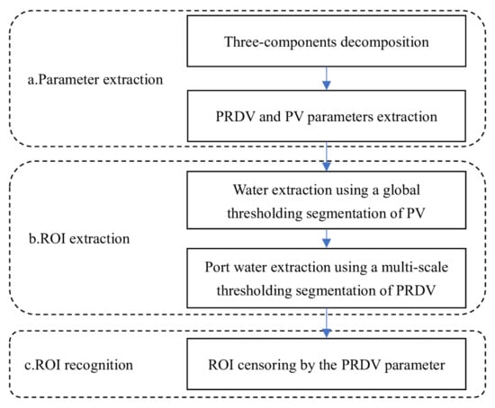
Figure 2.
Diagram of the proposed port detection method.
3.1. Polarimetric Parameters Extraction
As is known, the backscattering of the calm or low state water can be modeled as the Bragg surface scattering [30]. However, the scattering of water regions near a port or an urban area are different due to the interference of the surrounding man-made buildings or ships. The scattering components of the water regions near a port or an urban area are usually more complex than those of other normal water regions. As shown in Figure 3, the Pauli pseudocolor image of Zhanjiang is shown in Figure 3a, where the sampling regions are marked in red boxes. The Pauli pseudocolor images of the four sampling regions, including a calm water region, an interference water region near an urban area, an interference water region on a port, and a vegetation region, are shown in Figure 3b–e, respectively. We can observe that the color of the two interference water regions in Figure 3c,d is redder than that of the calm water. The histograms of the span of the three regions are shown in Figure 3f, where , , and denote the histogram of the calm water region, the interference water region, and the land region, respectively. Statistical results validate that the scattering power of the interference water region is much higher than that of the calm water region. The scattering power of the interference water region is less than that of the land region. In the remainder of the article, the interference water stands for water regions interfered with by buildings in an urban area or a port, the port water stands for water regions on a port, and the normal water stands for water regions opposite to the interference water.
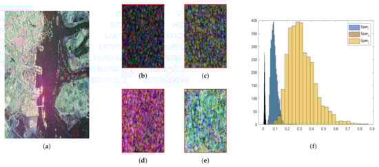
Figure 3.
The Pauli pseudocolor images and histograms of the sampled water and land regions: (a) The Pauli pseudocolor image of Zhanjiang, where the sampling regions are marked in red boxes; (b) a calm water region; (c) an interference water region near an urban area; (d) an interference water region in a port; (e) a vegetation land region; (f) the histograms of the span of the three sampling regions, where , , and denote the histogram of the calm water region, the interference water region, and the land region, respectively.
To analyze the scattering component of the port water, we obtain the Freeman-Durden three-component decomposition result of the sampled water regions in Figure 3 using (1). The histograms of normalized power , , and of the port water are shown in Figure 4a, where the three histograms are drawn in red, green, and blue, respectively. We can observe that the ratio of the scattering power of most pixels is larger than 0.5. Statistical results validate that the scattering component of the interference water is dominated by the double-bounce scattering component. This result is mainly caused by two factors. One is the sidelobe effect of strong scattering objects. Since the scattering power of strong scattering objects is dominated by double-bounce, the scattering component of the region interfered with by the sidelobe is also dominated by double-bounce scattering. The other is the double-bounce scattering components generated by the dihedral corner reflector between the strong scattering objects and the interference water. The scattering distribution of , , and components of the three different sampled water regions and the sampled land regions is shown in Figure 4b. Figure 4b shows that not only the water regions and the land region but also the three kinds of water regions are separable. To find out the distinct scattering component of the port water, the histograms of the scattering power of the port water are fitted using a gamma distribution. The histograms of the double-bounce powers of the normal water region and the interference water region are shown in Figure 4c and Figure 4d, respectively, where the red lines stand for the distribution fitting result. Comparing Figure 4c and Figure 4d, we can find that the minimum power of the interference water is far larger than the maximum power of the normal water. Thus, the interference water is easy to separate from the normal water using the double-bounce power.
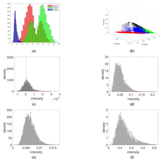
Figure 4.
The histograms of the double-bounce and the volume scattering powers of different sampled water and land regions where the distributions are fitting using a gamma distribution shown with a red line: (a) The histograms of normalized power , , and of the port water; (b) the scattering distribution of , , and components of the sampled water and land regions; (c) the double-bounce power of a normal water area; (d) the double-bounce power of an interference water area; (e) the volume power of an interference water area; (f) the volume power of a land area.
Although the double-bounce scattering power of the interference water is larger than that of the normal water, the difference in the volume scattering power between the interference water and the normal water is small since the interference component is dominated by double-bounce scattering. The volume scattering powers of both the interference water and normal water are all much lower than those of the land. The histograms of the volume scattering power of the interference water region and the land region are shown in Figure 4e,f, respectively. Comparing Figure 4e,f, we can observe that the minimum power of the vegetation region is far larger than the maximum power of the interference water. Thus, the water region can be separated from the land using the volume scattering power.
By a combination of the double-bounce power and the volume power , the interference water in the ports can be extracted from the image. However, a negative power problem exists in the Freeman decomposition. We can observe that the double-bounce powers of half of the sampled normal water pixels are negative from Figure 4c. To avoid the problem, we can obtain the double-bounce scattering power and volume scattering power using (6). The scattering distributions of the and of the sampled water and land regions are shown in Figure 5a. We can observe that the water regions and the land are separable using , and the interference water and calm water are separable using . However, the difference of between the interference water and calm water is small.
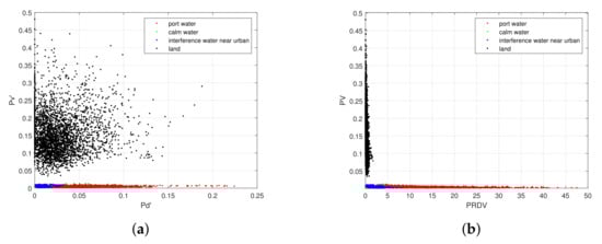
Figure 5.
The scattering distributions of the polarimetric parameters of the sampled regions: (a) the scattering distributions of the and of the sampled regions; (b) the scattering distributions of the PRDV and PV parameters of the sampled regions.
Except for the interference water regions, there are some land regions also interfered with by the surrounding man-made buildings or strong scatterers. If an interference land region is soil or another low scattering region, its volume scattering power is so low that it is segmented to a water region by the thresholding segmentation of . Since the average difference of the double-bounce scattering power between the interference land region and the interference water is small, it is difficult to identify the two regions using . To avoid a false result and enhance the contrast of between the interference water and the interference land region, the PRDV parameter is proposed to separate the interference water and the normal water. The parameter is defined as follows:
where denotes the double-bounce scattering power, and denotes the volume scattering power. Because the volume scattering power of the interference water region is lower than that of the interference land region, the PRDV parameter of the two kinds of regions is separable.
3.2. ROI Extraction
Using the parameters PRDV and PV, the ROI of ports can be extracted by detecting the port water region. Using the parameter PV, the water and land can be separated first. The interference water can then be separated from the normal water using the parameter PRDV.
Since the difference of PV between the water and the land is usually large, PV can be segmented using a global thresholding method such as Ostu or a region-based method such as level set segmentation. If the whole histogram of the image satisfies a two-peak distribution, correct segmentation can be easy to obtain using a two-region segmentation method. However, the two-peak distribution is difficult to satisfy since the land consists of the urban area, high vegetation, low vegetation, and soil, and the water consists of normal water and interference water. Thus, the global CFAR thresholding segmentation method is used to segment the water and land. In the method, the water is taken as a background, and the land is taken as a target. Unlike the traditional CFAR work in a sliding window with a constant size under a false alarm rate (FAR), the method has a threshold by fitting the distribution of the background in a sampling region but segments the whole image plane using that threshold. As the volume power is approximately equal to the power of the cross-polarization component according to (6), the probability distribution of the volume power of the water is fitted to a gamma distribution. However, samples from different water areas in different image scenes are needed to estimate the parameters of the average power and the equivalent number in the gamma distribution. If the sampling regions are only selected from the region of calm water, land cannot be detected regardless of how large the false alarm rate is set since the volume scattering power of the calm water is much lower than that of land. Statistical results shown in Figure 5a show that the difference of the average PV between the land and the calm water only varies in a certain range. Therefore, we propose to obtain the threshold by adding a constant to the average PV of a sampling water region.
To obtain the sampling region using an unsupervised approach, a patch of size in the center of the pixel is selected for each pixel. We then find the patch that the mean multiply variance is minimum. That is, the homogeneity measure of the mean and variance of the patch is defined as follows:
where is the mean, and is the variance of the span of a patch.
The patch with the smallest homogeneity is selected as the sampling region. If the average PV of the sampling region is , the threshold of PV for water extraction is then set as + C. Our statistical results show that C should be set in the interval from 5 to 10 dB.
Since the difference of the PRDV between the interference water and the normal water is large, the PRDV can also be segmented using the global CFAR method. However, the explicit probability density function (PDF) of the ratio parameter is difficult to deduce. Since the double-bounce power of the normal water is very low and the area percentage of the interference is very small, the PDF of the ratio parameter for the whole water region approximates a gamma distribution. Thus, the interference water can be detected by the global CFAR detection method, in which the interference water is taken as a target and the normal water is a background. However, the problem of the interference water extraction using the CFAR method is also that the sampling regions are difficult to obtain. The PDF of the PRDV parameter cannot be fitted using the same region as the water extraction because the value of the PRDV is close to zero in the normal water region. Thus, all the pixels of the water region are taken as samples for the PDF fitting of the PRDV parameter. Because the value of the PRDV of some interference water regions is far greater than that of other water regions, the pixels with the largest percentage of PRDV are removed from the sampling points first. The global threshold for the interference water extraction are then set by the CFAR method based on the fitted PDF.
The area of the interference water in a port is large since the number of man-made buildings and ships is large. Therefore, the ROI of the port can be extracted by finding the interference water with a large area. However, there are many isolated points in the CFAR detection result because the method only segments the water using a global threshold. To avoid the problem, global thresholding segmentation is carried out on multi-scale images. As shown in Figure 6, we obtain an image pyramid of the map of PRDV by downsampling first, where the downsampling is the same as the average pooling. Afterward, the suspicious interference water of the image in each scale is detected by global thresholding segmentation using the threshold . The detection result of the k-th scale is the sum of the thresholding segmentation result of the k-th scale and the detection result of the -th scale in a process of upsampling, which is computed by the nearest neighbor interpolation method. Finally, the detection result of the image in the primary scale is taken as the result of the final suspicious interference water. The connected region and the corresponding minimum external quadrilateral are extracted from the binary result. If the area of a connected region is larger than , its external quadrilateral is identified as an ROI of ports.
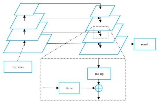
Figure 6.
The multi-scale thresholding segmentation for the extraction of the interference water, where ‘thres’ denotes the thresholding process, ‘mx down’ denotes m times downsampling, and ‘mx up’ denotes m times upsampling.
3.3. ROI Recognition
Because some land regions with low scattering intensity are also interfered with by surrounding buildings, there may be some false alarms in the extracted ROIs. The difference between the false alarm and the true target is that the double-bounce scattering power of the land in ports is much higher than that of the false alarm. The reason for this is that there are usually some metal structures with a strong scattering in ports. The area of the strong scattering region of the true target is also larger than that of the false alarms. Thus, the false alarms can be removed by the thresholding segmentation of the double-bounce scattering power and by calculating the area ratio of the strong double-bounce scattering region in the land of the extracted ROI. However, it is difficult to obtain the threshold because the sampling region is not available. Since the volume scattering power of the strong double-bounce scattering region is usually low, the PRDV parameter used for the interference water extraction can also be used for the extraction of the strong double-bounce scattering region in the land. Because the volume scattering power of the interference water is much smaller than that of the land region, the threshold obtained in the interference water extraction can also be used for this extraction.
For a candidate ROI, the land regions in the ROI are first extracted based on the water and land segmentation results. The strong double-bounce scattering region of the land in the ROI is then extracted by the thresholding segmentation result of PRDV using . If the area ratio of the strong scattering region to the land region in the ROI is smaller than the threshold, the ROI is recognized as a false alarm; otherwise, it is recognized as a detected port.
The extension of the interference water in a port may be far away from the land. To make the detected port closer to the true port, the minimum external quadrilateral of the land region in the ROI is finally recognized as the detected port.
4. Experimental Results and Analysis
The proposed method was tested with a number of single-look quad-polarization SAR images acquired by RADARSAT-2 at the coasts of Dalian, Zhanjiang, Fujian, Tianjin, Lingshui, and Boao in China and Berkeley in America. In the first experiment, the Dalian data were tested to show the detailed process flow of the proposed method. In the second experiment, the detection accuracy and robustness of the proposed method were demonstrated by six images with different coastal terrains and environments. In the third experiment, the performances of the proposed method were tested under different testing parameters using the Zhanjiang data. In the fourth experiment, the distribution fitting results and the calculated thresholds of the PRDV parameter were analyzed. In the fifth experiment, the detection performances of the proposed method were compared with the method of jetty scanning [7,8]. Finally, the time complexity of the proposed method was analyzed and compared with the method of jetty scanning. The computation time of each step of the proposed method was calculated. In all tests, the detection accuracy of a port was evaluated with the intersection of union section (IoU) index between the detected port and the ground truth. The ground truth of each data was drawn according to Google Earth maps. If the ground truth of a port was GT and the detected result of the port was DR, then the IoU index was defined as follows:
where denotes the union of regions of DR and GT, and denotes the intersection of the two regions.
The detailed parameters of the seven testing datasets are shown in Table 1. The range resolutions are all . The azimuth resolutions are varied from to . The image scene range is about , i.e., the size of the images is about . The angles of incident are varied from to .

Table 1.
Experimental dataset details, where ‘UTC’ stands for the international standard time, ‘AOI’ stands for the angle of incident, and stands for meter times meter.
To reduce the variance of the powers of three-component decomposition caused by the speckle, the testing data were filtered with a box-car filter first, where the window size is an empirical parameter. In the ROI extraction step, the constant C was set to 7 dB during the thresholding segmentation of the volume scattering power to extract water. The FAR was set to 0.05 during the thresholding segmentation of the PRDV to extract the interference water. The optimum value of the two parameters C and FAR are set by comparing the performance of the proposed method under different parameters using the data of Zhanjiang. The detailed experimental results are shown in the third experiment. The window size N for the sampling region selection of PV segmentation is set to 9, which can be set from 5 to a larger value. When the multi-scale thresholding segmentation method was used, the downsampling and upsampling rate m were set to 2. The number of layers of the scale was set to 4, where the number can be varied from 2 to 5. was set to 4000, assuming the length of the port was larger than 500 m and the width was larger than 200 m, and the values were obtained by making a statistic of the ground truth of the ports in the seven testing datasets. In the ROI recognition step, the area ratio was set to 0.1 because the strong double-bounce scattering region was only a small part of the total land region in the ROI.
4.1. Example Result
In the first experiment, single-look quad-polarization SAR images over Dalian were used to show the flow of the proposed method. The Pauli pseudocolor image of the data is shown in Figure 7a. We can observe that there is a bright red region in the center of the image. The region is the target port, in which the water is seriously interfered with by the surrounding man-made buildings and metal structures. The intermediate results of the proposed method are shown in Figure 7b–f. The image of the parameter PV is shown in Figure 7b. There is a red bright box in the water region of Figure 7b, which is the selected rectangle sampling region according to (8). The image of the parameter PRDV is shown in Figure 7c. Figure 7b shows that the PV of the water is much smaller than that of the land. Figure 7c shows that the PRDV parameter of the interference water is much larger than that of the normal water. We can also see that the difference of the PRDV parameter between the strong scattering region and the other regions in land is large. The water extraction result is shown in Figure 7d. Both the interference water and other normal water are well separated from the land. The interference water extraction result is shown in Figure 7e, where the extracted water pixels are drawn in gray, the detected interference water pixels are drawn in white, and the extracted ROI is marked with a red box. We can observe that the interference water is well separated from the normal water, but the extension of the extracted ROI is far away from the land of the target port. The ROI recognition result is shown in Figure 7f, where the final detected port is marked with a red box. We can see that the detected port is close to the true target port after the post-processing of the ROI.
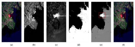
Figure 7.
Port detection result of Dalian data: (a) the Pauli pseudocolor image; (b) the image of volume scattering power; (c) the image of the ratio of the double-bounce scattering power to the volume scattering power; (d) the water extraction result; (e) the interference water extraction result, where the extracted water pixels are drawn in gray, the detected interference water pixels are drawn in white, and the extracted ROI is marked with a red box; (f) the ROI recognition result, where the detected port is marked with a red box.
4.2. Tests in Different Coastal Scenes
In the second experiment, a set of single-look quad-polarization SAR images were used to evaluate the proposed method, including the coasts of Zhanjiang, Fujian, Tianjin, Lingshui, and Boao in China and Berkeley in America. The Pauli pseudocolor images of the data are shown in Figure 8a1–f1. We can see that there is a port in each image, except in the Boao data. The area of water interfered with by the port is large in Zhanjiang, Berkeley, and Tianjin. In Zhanjiang, Fujian, and Lingshui, there is a wide intertidal flat, which makes the water difficult to be separated from the land. The area of the port is large in Tianjin but is small in Fujian. There are many small harbors in Zhanjiang and Tianjin. The target ports are difficult to identify from harbors if the geometric method is used. The target port in Fujian is difficult to detect because the interference water is narrow. The ROI extraction results are shown in Figure 8a2–f2. We can see that almost all interference water regions are correctly detected from the results. The extracted ROI in each image correctly covers the target port, except in Boao. The ROI recognition results are shown in Figure 8a3–f3, where the detected port is marked in a red box and the ground truth is marked in a green box. Compared with Figure 8a2–f2, we can see that the covering boxes are more accurate due to the process of land region location. The false alarm detected in Boao is correctly removed by the process of ROI censoring in Figure 8f3. The zooming recognition results near the target ports are shown in Figure 8a4–f4. We can see that all the detected ports are close to the ground truth. The IoU indexes are listed in Table 2. The largest value is 77.8% in the Berkeley data, while the smallest value is 44.18% in the Lingshui data. The indexes of Zhanjiang and Berkeley are both larger than 75%. All the indexes are larger than 50%, except the smallest value.
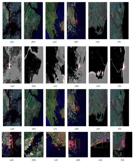
Figure 8.
Detection results in different coastal scenes: (a1–f1) The Pauli pseudocolor image of Zhanjiang, Fujian, Tianjin, Lingshui, and Boao in China and Berkeley in America; (a2–f2) the ROI etection result, where the extracted water pixels are drawn in gray, the detected interference water pixels are drawn in white, and the extracted ROI is marked in red boxes; (a3–f3) the ROI recognition dresult, where the detected port is marked in a red box and the ground truth is marked in a green box; (a4–f4) the zooming recognition result near the target port; (a1–a4) Zhanjiang; (b1–b4) Fujian; (c1–c4) Berkeley; (d1–d4) Tianjin; (e1–e4) Lingshui; (f1–f4) Boao.
Table 2.
The IoU indexes of the proposed method under different coastal scenes.
4.3. Tests in Different Parameters
In the third experiment, the performances of the proposed method were tested under different testing parameters using the Zhanjiang data. Because the performance of the proposed method is mainly affected by the thresholds of PV and PRDV parameters, the proposed method was tested under different C and FAR values. To evaluate how the performance varies under different PV thresholds, FAR was set to a constant of 0.05, and C was set to 5, 7, and 9 dB. The detection result is shown in Figure 9, where the first column in Figure 9a1–a3 corresponds to the C set to 5 dB, the second column in Figure 9b1–b3 corresponds to 7 dB, and the third column in Figure 9c1–c3 corresponds to 9 dB. The water and land segmentation results are shown in Figure 9a1–c1. Figure 9a1–c1 shows that the ratio of water pixels increases as value C increases. The ROI extraction results are shown in Figure 9a2–c2. Comparing Figure 9b2 with Figure 9a2, we can see that more water pixels are detected as an ROI in Figure 9a2. The reason for this is that the number of water pixels wrongly segmented to land increases with the decrease of C. Comparing Figure 9b2 with Figure 9c2, we can see that more land pixels are detected as an ROI in Figure 9c2. The reason for this is that the number of land pixels wrongly segmented to water increases with the increase of C. The ROI recognition results are shown in Figure 9a3–c3. We can see that the detected result in Figure 9b3 has the smallest difference from the ground truth. The IoU indexes are listed in the second row of Table 3. The highest value is 75.38% when C is set to 7 dB, but the value is 58.91% when C equals 5 dB and 54.09% when C equals 9 dB.
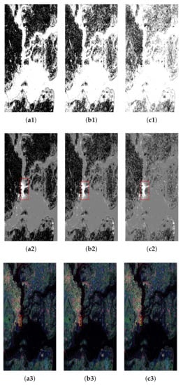
Figure 9.
Comparison of the proposed method under different PV thresholds in the Zhanjiang data: (a1–a3) C is set to 5 dB; (b1–b3) C is set to 7 dB; (c1–c3) C is set to 9 dB; (a1–c1) the water and land segmentation results; (a2–c2) the ROI extraction results; (a3–c3) the ROI recognition results.
Table 3.
The IoU indexes of the proposed method under different C and FAR parameters.
To evaluate how the performance is varied under different PRDV thresholds, C was set to a constant of 7 dB and FAR was set to 0.02, 0.05, and 0.09. The detection result is shown in Figure 10, where the first column in Figure 10a1–a3 corresponds to a FAR set to 0.02, the second column in Figure 10b1–b3 corresponds to 0.05, and the third column in Figure 10c1–c3 corresponds to 0.09. The interference water segmentation results are shown in Figure 10a1–c1. Figure 10a1–c1 shows that the ratio of the interference water pixels increases with the increase of FAR. The ROI extraction results are shown in Figure 10a2–c2. Comparing Figure 10c2 with Figure 10a2 and Figure 10b2, we can find that more interference water pixels are detected as an ROI in Figure 10c2. The reason for this is that the number of normal water pixels wrongly segmented to the interference water increases with the increase of FAR. The ROI recognition results are shown in Figure 10a3–c3. We can see that the offsets between the detected ports and the ground truth in Figure 10a3 and Figure 10b3 are small. The IoU indexes are listed in the fourth row of Table 3. The highest value is 75.94% when FAR is set to 0.02, but the value is 61.91% when FAR equals 0.09. The value of 75.38%, when FAR equals 0.05, is almost the highest value.
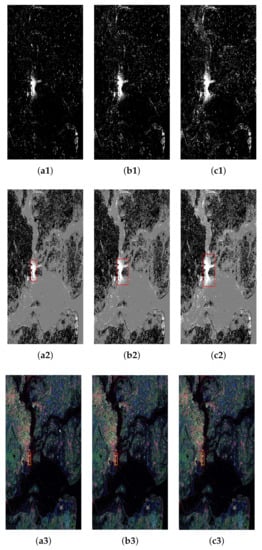
Figure 10.
Comparison of the proposed method under different PRDV thresholds in the Zhanjiang data: (a1–a3) FAR is set to 0.02; (b1–b3) FAR is set to 0.05; (c1–c3) FAR is set to 0.09; (a1–c1) the water and land segmentation results; (a2–c2) the ROI extraction results; (a3–c3) the ROI recognition results.
4.4. Threshold Determination and Distribution Fitting
In the fourth experiment, the distribution fitting results and the calculated thresholds of the PRDV parameter were analyzed. The fitting results of the PRDV parameter are shown in Figure 11. Figure 11a–d shows the results of the Zhanjiang, Fujian, Berkeley, and Tianjin data, respectively, where the fitted gamma distributions are drawn with a red line. We can see that the histograms of the four data are all well fitted with a gamma distribution. The calculated thresholds are listed in Table 4, where the values of the first row stand for the average PV power of the sampling region selected by (8), the second row shows the calculated PV thresholds, the third row shows the average PRDV parameters of the extracted water region, and the fourth row shows the calculated thresholds of the PRDV parameter. The table shows that the PV thresholds of Fujian, Berkeley, and Tianjin, which are 0.0114, 0.0081, and 0.007, are almost equal, but the threshold of Zhanjiang is much larger. The reason for this is that there are many tanks on the sea in the Zhanjiang data. The thresholds of the PRDV parameter in Zhanjiang and Tianjin, which are 3.243 and 2.854, are larger than the thresholds in Fujian and Berkeley, which are 1.502 and 1.950. The reason for this is that the interference is more serious in Zhanjiang and Tianjin.
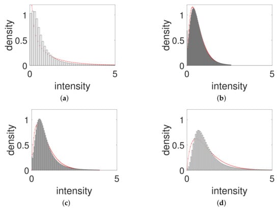
Figure 11.
The distribution fitting results of the ratio parameter in different scenes, where the fitted gamma distributions are drawn with a red line: (a) Zhanjiang; (b) Fujian; (c) Berkeley; (d) Tianjin.
Table 4.
Thresholds of the PV and PRDV in the Zhanjiang, Fujian, Berkeley, and Tianjin data, where denotes the average volume power of the sampling region, and denotes the average ratio parameter in the extracted water region.
4.5. Performance Comparison with Jetty Scanning Method
In the fifth experiment, the proposed method was compared with the port detection method based on jetty scanning [7,8], where the water extraction result detected by the thresholding segmentation of PV parameters in the proposed method was used in the jetty scanning method. Zhanjiang, Fujian, and Berkeley data were used for the test. Because a connected water–land segmentation result is needed to perform jetty scanning, the water extraction result was first processed by small area removal. The detection results are shown in Figure 12. The water–land segmentation results of the proposed method are shown in Figure 12a1–c1. The detection results of the proposed method are shown in Figure 12a2–c2. The water–land segmentation results obtained by the process of small area removal are shown in Figure 12a3–c3. We can see that the processed water–land segmentation result is wrong in the Zhanjiang data because of the wide intertidal flat in Figure 12a3. There are some wrong segmentation pixels along the cross-sea bridge due to the scattering interference in Berkeley in Figure 12c3. The detection results of the comparison method are shown in Figure 12a4–c4. For the comparison method, there are many false alarms with the Zhanjiang data due to the wrong water–land segmentation result in Figure 12a4. There are many false alarms with the Fujian and Berkeley data due to the natural protruding terrain along the coast in Figure 12b4,c4. The number of false alarms and the IoU index of the comparison method and the proposed method are listed in Table 5. The table shows that the numbers of false alarms of the comparison methods are 72, 17, and 16, and the IoU values of the detected target port are 25.18%, 1.36%, and 17.4% for the three data, respectively. Compared with the proposed method, the number of false alarms of the comparison method is much larger, and the IoU value is much lower. We can conclude that the performance of the proposed method is much better since all ports are correctly detected and no false alarms are detected by the proposed method.
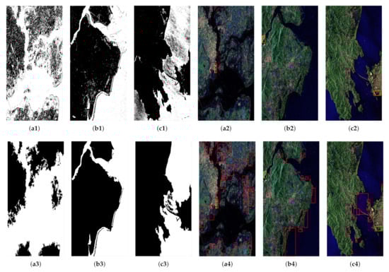
Figure 12.
Performance comparison of the proposed method with the jetty scanning method in the Zhanjiang, Fujian, and Berkeley data, where the detected targets are marked with a red box, and the ground truth is marked in a green box: (a1–c1) the water and land segmentation results; (a2–c2) the port detection of the proposed method in the Zhanjiang, Fujian, and Berkeley data; (a3–c3) the water–land segmentation results obtained by the process of small area removal; (a4–c4) the port detection of the jetty scanning method; (a1–a4) Zhanjiang; (b1–b4) Fujian; (c1–c4) Berkeley.
Table 5.
Performance comparison of the proposed method with the jetty scanning method, where ‘FA’ stands for the number of false alarms.
4.6. Time Complexity Analysis
The time-consuming steps of the proposed algorithm mainly include the polarimetric parameter calculation, sampling region selection, port water extraction, and ROI recognition. For the parameter calculation, if the size of the image is , the time complexity is , since each pixel only needs to perform several additions and multiplications. For the sampling region selection, if the window size is N, the time complexity is . For the port water extraction, if the size of the image is , the layer of scale is k, and the time complexity of the image pyramid construction is . However, all pixels in the image plane can be computed in parallel during the three steps of parameter calculation, sampling region selection, and port water extraction. Therefore, the time complexity of these three steps is low if all pixels are computed in parallel. The computation time of the ROI recognition steps is trivial as only PDF fitting and connection region extraction are computed. The computation times of each step are listed in Table 6, where the testing platform is Matlab v9.5, and the CPU is Intel Xeon at 3.6 GHz with 16 GB RAM. The times of the polarimetric parameter calculation are 49.8 s, 37.8 s, and 22.0 s with the Zhanjiang, Fujian, and Berkeley data, respectively. The total times are 101.6 s, 80.8 s, and 55.5 s, respectively. Compared with the proposed method, the time-consuming steps of the comparison method include the water–land segmentation post-processing and jetty scanning, but not the step of water–land segmentation. The total times are 447.93 s, 123.9 s, and 101.35 s, respectively, using the three datasets. The total time of the proposed method is less than that of the comparison method. The time complexity of the proposed method is low because accurate coastline detection and sophisticated geometric feature extraction are not needed.
Table 6.
Computation time of the proposed method, where ‘Pol’ stands for the polarimetric parameter calculation, and ‘Sa’ stands for sampling region selection.
5. Conclusions
A port detection method in polarimetric SAR images has been proposed by extracting the special interference water in ports using the volume scattering power and the ratio of double-bounce to volume scattering power based on the improved three-component decomposition. Port water is an important component of a port in polarimetric SAR images. Due to a special scattering component of the water in a port, the water appears differently from other water. Thus, water can be separated from land using the volume scattering power, and the interference water in a port can then be separated from normal water by the power ratio parameter using the multi-scale thresholding segmentation method. By extracting the special scattering component based on polarization decomposition, port water is easy to detect. Because the detection steps are independent of the accuracy of the coastline extraction and the geometric feature extraction of the contours of the port, the proposed method has a low time complexity and a high accuracy. The experimental results of the seven polarimetric data acquired by RADARSAT-2 over the coasts of Dalian, Zhanjiang, Fujian, Tianjin, Lingshui, and Boao in China and Berkeley in America demonstrated the effectiveness of the proposed method. All ports can be fast and accurately detected by the proposed method. Compared with the method based on jetty scanning, no false alarms are detected, and the IoU indexes of the detected port are much higher in the proposed method.
6. Patents
An earlier version of this work was authorized with the patent ZL201510998952.1, “Port water area extraction based large port detection method for polarimetric SAR image”, in 2018.
Author Contributions
Conceptualization, C.L. and J.Y.; methodology, C.L.; software, C.L.; validation, C.L., J.Z. and X.N.; formal analysis, J.Y.; investigation, J.Z.; resources, J.Y.; data curation, X.N.; writing—original draft preparation, C.L.; writing—review and editing, J.Y.; visualization, C.L.; supervision, J.Y.; project administration, C.L.; funding acquisition, C.L. and J.Y. All authors have read and agreed to the published version of the manuscript.
Funding
This work was in part supported by the National Natural Science Foundation of China (NSFC) (No. 62101456 and 62171023), supported in part by the Fundamental Research Funds for the Central Universities (No. D5000210752).
Institutional Review Board Statement
Not applicable.
Informed Consent Statement
Not applicable.
Data Availability Statement
Please contact Chun Liu (liuchun@nwpu.edu.cn) for access to the data.
Acknowledgments
The authors would like to thank the reviewers for their valuable comments and suggestions. The data were provided by the lab of polarimetric radar & remote sensing applications of Tsinghua University and the China National Satellite Ocean Application Service.
Conflicts of Interest
The authors declare that there is no conflict of interest regarding the publication of this paper.
References
- Liu, C.; Zheng, J.; Nie, X. Port Detection in Polarimetric SAR Images Based on Three-Component Decomposition. In Proceedings of the IGARSS 2020 IEEE International Geoscience and Remote Sensing Symposium, Waikoloa, HI, USA, 26 September–2 October 2020; pp. 734–737. [Google Scholar]
- Liu, C.; Xiao, Y.; Yang, J. Harbor Detection in Polarimetric SAR Images Based on the Characteristics of Parallel Curves. IEEE Geosci. Remote Sens. Lett. 2016, 13, 1400–1404. [Google Scholar] [CrossRef]
- Liu, C.; Yin, J.; Yang, J. Small harbor detection in polarimetric SAR images based on coastline feature point merging. J. Tsinghua Univ. Sci. Technol. 2015, 55, 849–853. [Google Scholar]
- Li, Y.; Peng, J. Feature extraction of the harbor target and its recognition. J. Huazhong Univ. Sci. Technol. 2001, 29, 10–12. [Google Scholar]
- He, J.; Guo, Y.; Zhang, Z.; Yuan, H.; Ning, Y.; Shao, S. Harbor Extraction Based on Edge-Preserve and Edge Categories in High Spatial Resolution Remote-Sensing Images. Appl. Sci. 2019, 9, 420. [Google Scholar] [CrossRef] [Green Version]
- Chen, Q.; Lu, J.; Zhao, L.; Kuang, G. Harbor Detection Method of SAR Remote Sensing Images Based on Feature. J. Electron. Inf. Technol. 2010, 32, 2873–2878. [Google Scholar] [CrossRef]
- Zhao, H.; Li, W.; Yu, N.; Ao, H. Harbor detection in remote sensing images based on feature fusion. In Proceedings of the 5th International Congress Image Signal Process, Chongqing, China, 16–18 October 2012; pp. 1053–1057. [Google Scholar]
- Liu, C.; Yang, J.; Xie, C.; An, W.; Yuan, X. Man-made harbor detection in polarimetric SAR images based on multi-direction jetties scanning. J. Syst. Eng. Electron. 2017, 39, 291–297. [Google Scholar]
- Wang, R.; Xu, F.; Zhang, Q.; Pei, J.; Huang, Y.; Yang, J. Harbor Detection in SAR Images Based on Multidirectional One-Dimensional Scanning. In Proceedings of the IGARSS 2020 IEEE International Geoscience and Remote Sensing Symposium, Waikoloa, HI, USA, 26 September–2 October 2020; pp. 1–4. [Google Scholar]
- Liu, C.; Yang, J.; Yin, J.; An, W. Coastline detection in SAR images using a hierarchical level set segmentation. IEEE J. Sel. Topics Appl. Earth Observ. Remote Sens. 2016, 9, 4908–4920. [Google Scholar] [CrossRef]
- Schmitt, M.; Baier, G.; Zhu, X. Potential of nonlocally filtered pursuit monostatic TanDEM-X data for coastline detection. ISPRS J. Photogramm. Remote Sens. 2019, 148, 130–141. [Google Scholar] [CrossRef] [Green Version]
- Liu, C.; Xiao, Y.; Yang, J. A Coastline Detection Method in Polarimetric SAR Images Mixing the Region-Based and Edge-Based Active Contour Models. IEEE Trans. Geosci. Remote Sens. 2017, 55, 3735–3747. [Google Scholar] [CrossRef]
- Modava, M.; Akbarizadeh, G.; Soroosh, M. Integration of spectral histogram and level set for coastline detection in SAR images. IEEE Trans. Aerosp. Electron. Syst. 2019, 55, 810–819. [Google Scholar] [CrossRef]
- Rosenfeld, A.; Johnston, E. Angle Detection on Digital Curves. IEEE Trans. Comput. 1973, 22, 875–878. [Google Scholar] [CrossRef]
- Douglas, D.H.; Peucker, T.K. Algorithms for the reduction of the number of points required to represent a digitized line or its caricature. Cartogr. Int. J. Geogr. Inf. Geovis. 1973, 10, 112–122. [Google Scholar] [CrossRef] [Green Version]
- Wang, W.; Yang, X.; Li, X.; Chen, K.; Liu, G.; Li, Z.; Gade, M. A Fully Polarimetric SAR Imagery Classification Scheme for Mud and Sand Flats in Intertidal Zones. IEEE Trans. Geosci. Remote Sens. 2017, 55, 1734–1742. [Google Scholar] [CrossRef]
- Ferrentino, E.; Buono, A.; Nunziata, F.; Marino, A.; Migliaccio, M. On the Use of Multipolarization Satellite SAR Data for Coastline Extraction in Harsh Coastal Environments: The Case of Solway Firth. IEEE J. Sel. Top. Appl. Earth Observ. Remote Sens. 2021, 14, 249–257. [Google Scholar] [CrossRef]
- Girshick, R.; Donahue, J.; Darrell, T.; Malik, J. Rich feature hierarchies for accurate object detection and semantic segmentation. In Proceedings of the CVPR 2014 IEEE Conference on Computer Vision and Pattern Recognition, Columbus, OH, USA, 23–28 June 2014; pp. 580–587. [Google Scholar]
- Ren, S.; He, K.; Girshick, R.; Sun, J. Faster R-CNN: Towards real-time object detection with region proposal networks. IEEE Trans. Pattern Anal. Mach. Intell. 2017, 39, 1137–1149. [Google Scholar] [CrossRef] [PubMed] [Green Version]
- He, K.; Gkioxari, G.; Dollár, P.; Girshick, R. Mask R-CNN. IEEE Trans. Pattern Anal. Mach. Intell. 2020, 42, 386–397. [Google Scholar] [CrossRef]
- Freeman, A.; Durden, S.L. A three-component scattering model for polarimetric SAR data. IEEE Trans. Geosci. Remote Sens. 1998, 36, 963–973. [Google Scholar] [CrossRef] [Green Version]
- Yamaguchi, Y.; Moriyama, T.; Ishido, M.; Yamada, H. Four-component scattering model for polarimetric SAR image decomposition. IEEE Trans. Geosci. Remote Sens. 2005, 43, 1699–1706. [Google Scholar] [CrossRef]
- Cloude, S.R.; Pottier, E. An entropy based classification scheme for land applications of polarimetric SAR. IEEE Trans. Geosci. Remote Sens. 1997, 35, 68–78. [Google Scholar] [CrossRef]
- Chen, J.; Chen, Y.; Yang, J. Ship detection using polarization Cross-Entropy. IEEE Geosci. Remote Sens. Lett. 2009, 6, 723–727. [Google Scholar] [CrossRef]
- Yang, J.; Zhang, H.; Yamaguchi, Y. GOPCE-Based approach to ship detection. IEEE Geosci. Remote Sens. Lett. 2012, 9, 1089–1093. [Google Scholar] [CrossRef]
- Yang, J.; Peng, Y.N.; Lin, S.M. Similarity between two scattering matrices. Electron. Lett. 2001, 37, 193–194. [Google Scholar] [CrossRef]
- Touzi, R.; Hurley, J.; Vachon, P.W. Optimization of the degree of polarization for enhanced ship detection using polarimetric RADARSAT-2. IEEE Trans. Geosci. Remote Sens. 2015, 53, 5403–5424. [Google Scholar] [CrossRef]
- An, W.; Cui, Y.; Yang, J. Three-Component Model-Based Decomposition for Polarimetric SAR data. IEEE Trans. Geosci. Remote Sens. 2010, 48, 2732–2739. [Google Scholar]
- Lee, J.S.; Schuler, D.L.; Ainsworth, T.L.; Krogager, E.; Kasilingam, D.; Boerner, W. On the estimation of radar polarization orientation shifts induced by terrain slopes. IEEE Trans. Geosci. Remote Sens. 2002, 40, 30–41. [Google Scholar]
- Lee, J.S.; Schuler, D.L. Mapping ocean surface features using biogenic slick-fields and SAR polarimetric decomposition techniques. IEE Proc.-Radar Sonar Navig. 2006, 153, 260–270. [Google Scholar]
Publisher’s Note: MDPI stays neutral with regard to jurisdictional claims in published maps and institutional affiliations. |
© 2022 by the authors. Licensee MDPI, Basel, Switzerland. This article is an open access article distributed under the terms and conditions of the Creative Commons Attribution (CC BY) license (https://creativecommons.org/licenses/by/4.0/).