Article

Spectral Temporal Information for Missing Data Reconstruction (STIMDR) of Landsat Reflectance Time Series

by
Zhipeng Tang
1,2,*,
Giuseppe Amatulli
3,4,
Petri K. E. Pellikka
1,2 and
Janne Heiskanen
1,2
1
Department of Geosciences and Geography, University of Helsinki, P.O. Box 68, 00014 Helsinki, Finland
2
Institute for Atmospheric and Earth System Research, Faculty of Science, University of Helsinki, 00014 Helsinki, Finland
3
School of the Environment, Yale University, New Haven, CT 06511, USA
4
Center for Research Computing, Yale University, New Haven, CT 06511, USA
*
Author to whom correspondence should be addressed.
Remote Sens. 2022, 14(1), 172; https://doi.org/10.3390/rs14010172
Submission received: 24 November 2021 / Revised: 21 December 2021 / Accepted: 28 December 2021 / Published: 31 December 2021
(This article belongs to the Special Issue Satellite Image Processing and Applications)

Abstract

:
The number of Landsat time-series applications has grown substantially because of its approximately 50-year history and relatively high spatial resolution for observing long term changes in the Earth’s surface. However, missing observations (i.e., gaps) caused by clouds and cloud shadows, orbit and sensing geometry, and sensor issues have broadly limited the development of Landsat time-series applications. Due to the large area and temporal and spatial irregularity of time-series gaps, it is difficult to find an efficient and highly precise method to fill them. The Missing Observation Prediction based on Spectral-Temporal Metrics (MOPSTM) method has been proposed and delivered good performance in filling large-area gaps of single-date Landsat images. However, it can be less practical for a time series longer than one year due to the lack of mechanics that exclude dissimilar data in time series (e.g., different phenology or changes in land cover). To solve this problem, this study proposes a new gap-filling method, Spectral Temporal Information for Missing Data Reconstruction (STIMDR), and examines its performance in Landsat reflectance time series. Two groups of experiments, including 2000 × 2000 pixel Landsat single-date images and Landsat time series acquired from four sites (Kenya, Finland, Germany, and China), were performed to test the new method. We simulated artificial gaps to evaluate predicted pixel values with real observations. Quantitative and qualitative evaluations of gap-filled images through comparisons with other state-of-the-art methods confirmed the more robust and accurate performance of the proposed method. In addition, the proposed method was also able to fill gaps contaminated by extreme cloud cover for a period (e.g., winter in high-latitude areas). A down-stream task of random forest supervised classification through both gap-filled simulated datasets and the original valid datasets verified that STIMDR-generated products are relevant to the user community for land cover applications.

Graphical Abstract

1. Introduction

Time series has become the dominant form of remote sensing data for monitoring changes on the land surface [1,2]. Since the launch of the first Landsat sensor in 1972, Landsat satellites have observed changes in the land surface from space and have made the longest medium-resolution time series available for free [3,4]. The long archive, together with other satellites such as Sentinel-2, is a valuable resource for various applications, ranging from long-term land use and land cover (LULC) monitoring [5,6] and burned area estimation [7] to crop monitoring [8] and characterization of land-surface phenology [9] over shorter periods.
However, Landsat time-series applications are limited by missing observations (i.e., gaps), which continue to be a major obstacle, particularly when a dense time series is required [10]. This has stimulated research to reconstruct missing values and to produce gap-free imagery [10]. Reconstructing gap-free Landsat images in a time series is often more challenging than reconstructing single-date images for additional considerations of time series features.
One of the key factors is the number of valid (cloud-free) observations in the time series, which depends on satellite orbit and sensor geometry, clouds, and sensor issues [11]. Landsat has a 16-day revisit cycle; thus, a single Landsat sensor acquires approximately 23 scenes from 1 path and row per year. The number of observations can be greater if several Landsat sensors are available or if the pixel is covered by several Landsat paths. However, because of clouds and cloud shadows (CCS), the number of valid observations per pixel is typically considerably less than 23. Cloud cover can also be extremely high in some cases, for example, larger than 90% in the tropics during the wet season [12].
Gaps can be small or large in area and temporally and spatially irregular, which is another key factor that should be considered in reconstructing Landsat time series. For example, gaps resulting from Landsat 7 ETM+ Scan Line Corrector (SLC) failure are in a wedge shape [13]. Gaps resulting from continuous cloud cover are often irregular and large in area.
The methods to reconstruct SLC-off gaps are relatively well established [3,13,14,15]. However, gaps caused by CCS with greater temporal and spatial irregularity are more challenging to reconstruct. For time-series processing, spatial-based, temporal-based, and hybrid methods (i.e., those that use more than one of the spectral, spatial, and temporal information sources) are commonly developed in recovering various types of gaps [16,17,18], e.g., state-of-the-art methods that belong to these types are reviewed in Section 2.
In this work, we propose a novel gap-filling method named Spectral Temporal Information for Missing Data Reconstruction (STIMDR). To implement STIMDR, a pre-imputation for the image that is to be reconstructed is required. There are four main steps in STIMDR. The first step is to calculate the weight based on the spectral and temporal information (Section 3.2.2). Secondly, Section 3.2.3 describes how to find the most similar observations per pixel over the time series in the pre-imputation image based on spectral and temporal criteria. Thirdly, weighted STMs are calculated using the most similar observations and their weights (Section 3.2.4). Finally, the k-NN regression is used to predict the gap pixels based on the weighted STM feature space (Section 3.2.5). The new proposed method is suited to global implementation subject to a proper tuning procedure, which was provided by the sensitivity test varying from site to site.

2. Related Work

2.1. Spatial-Based Methods

Spatial-based methods assume that the missing data can be reconstructed from the valid data with similar spatial autocorrelation or geometrical structure by means of similar contextual information from the adjacent cloudy regions, e.g., moving window [13]. Such methods include diffusion methods [19], variation-based methods [20], and geostatistical kriging methods [21]. A recently proposed ordinary kriging gap-filling displayed good performance in marine remote sensing using miscellaneous and variant environmental datasets [22]. The spatial-based methods often take into account correlations in the spatial domain (local and nonlocal correlations), which can be severely dependent on the size of the gaps and the similarity of contextual structures [23]. Due to the spatial variation of the land cover and thus of the spectral signal, they are typically suitable for recovering small-area gaps and ineffective for large-scale cloud cover or complicated applications [24].

2.2. Temporal-Based Methods

Temporal-based methods, which employ time-series information, have the potential to reconstruct even the largest gaps without the influence of surrounding pixels. The representative methods consist of linear and spline interpolations. Akima spline interpolation [25,26] is based on a piecewise function composed of a set of polynomials, third degrees at most, producing a curve of given points with a successive interval that tends to have a natural look or resemble manual drafting [27]. It has been commonly applied to interpolating missing values in satellite imagery [28,29,30]. A drawback of Akima spline interpolation is that single noise-like (e.g., cloud-contaminated pixels) observations can result in large changes in the interpolation curve [31].
Steffen spline, a one-dimensional monotonic interpolation based on piecewise cubic functions [31], is an alternative interpolator. It has proved to be a stable and well-behaved interpolation method for time-series applications [32,33]. However, Steffen spline may have issues recovering peak and trough values by interpolating monotonic curves between each interval. Akima spline and Steffen spline methods are accessible from an open-source software Processing Kernel for geospatial data (Pktools) [34,35], written in C++ and relying on the GDAL API.
In addition, as another open-source project for state-of-the-art remote sensing, Orfeo Toolbox (OTB) provides a spline gap-filling method [36,37,38,39], which has received strong interest [40,41]. It combines linear and spline methods depending on the number of valid dates in the temporal profile. Orfeo Toolbox, together with Pktools, provides fast, flexible, and scalable features and functions for raster-based workflows with language integration using Bash or Python [42]. They also enable multi-core parallel processing of very large datasets owing to efficient algorithms and optimized memory management.

2.3. Hybrid Methods

Hybrid methods have been particularly successful in filling different types of gaps [43,44]. A popular hybrid method is the window regression (WR) method [14,45], which employs linear regression on the data selected within a spatial neighborhood of the gaps and in the temporal domain close to the date of the gaps (i.e., a spatial-temporal window). It has good performance in recovering Landsat ETM+ SLC-off data and MODIS NDVI time series. However, the spatial window-based models often have difficulties in recovering pixels that have heterogeneous land cover in the neighborhood, especially for coarser spatial resolution analysis [46].
Spatial coherence and temporal seasonal regularity was used in a gap-filling method that performed well in test sets featuring with 20% and 50% gaps [47]. This method was developed in four steps: (i) the adaptive selection of spatio-temporal neighborhood of the gaps, (ii) ranking of the subset temporal images, (iii) the estimation of empirical quantiles characterizing gaps, and (iv) quantile regression predicting the gaps. The method is available as an open-source R package, namely, gapfill. It contains the C++ source code and enables parallel computation in an R environment. gapfill may recover large-area gaps, but its efficiency decreases as the number of gap-filling routine repeats increases due to the large size of gaps [48].
Spectral-Angle-Mapper-based Spatio-Temporal Similarity (SAMSTS) was proposed to fill large-area gaps [10], and a fill-and-fit approach was used to predict within-year satellite time series spatially and temporally [49]. However, the segmentation process involved in SAMSTS can produce unwanted values [18].
Missing Observation Prediction based on Spectral-Temporal Metrics (MOPSTM) was developed to recover large-area gaps in Landsat images [18,50]. MOPSTM uses a k-Nearest Neighbor (k-NN) machine-learning method to predict missing observations based on the valid pixels in the target image and statistical spectral-temporal metrics (STMs) computed for a 1-year period as feature space [50]. MOPSTM may be sensitive to the time period. A 1-year period may obtain insufficient valid observations or even zero observations; however, a longer time period is more likely to include noise and dissimilar pixels (e.g., difference in phenology or changes in land cover).
A new branch of hybrid methods that includes deep learning theories has been the subject of great interest [24,51]. From the perspective of nonlinear expression ability of deep learning theory, hybrid methods involving spatial–temporal–spectral information have developed to recover images contaminated with dead pixels and thick clouds [24,52].
For example, the limitations of the state-of-the-art methods reviewed above are summarized in Table 1.

3. Materials and Methods
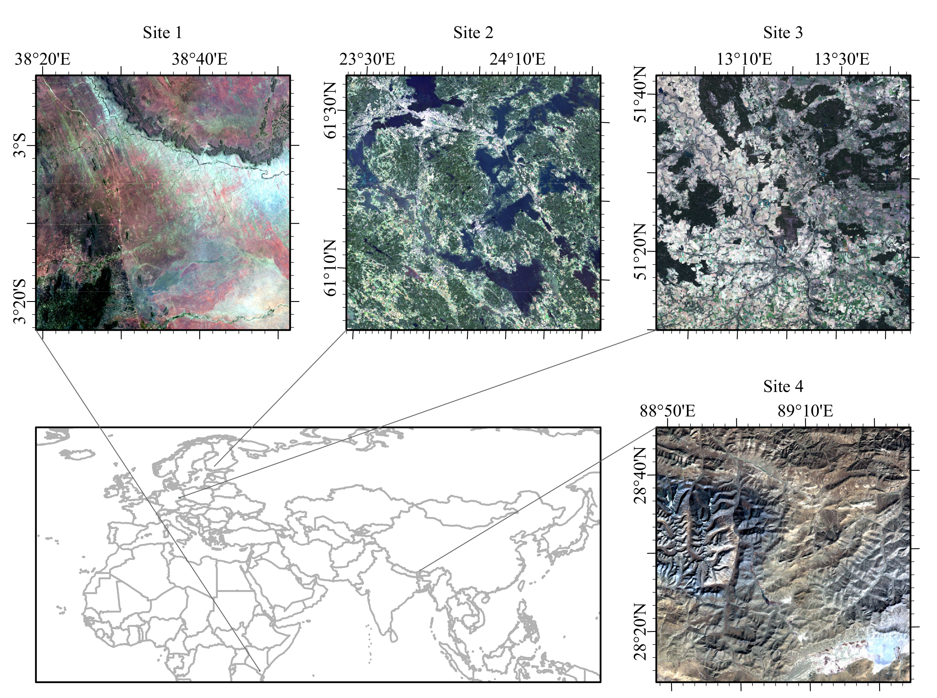
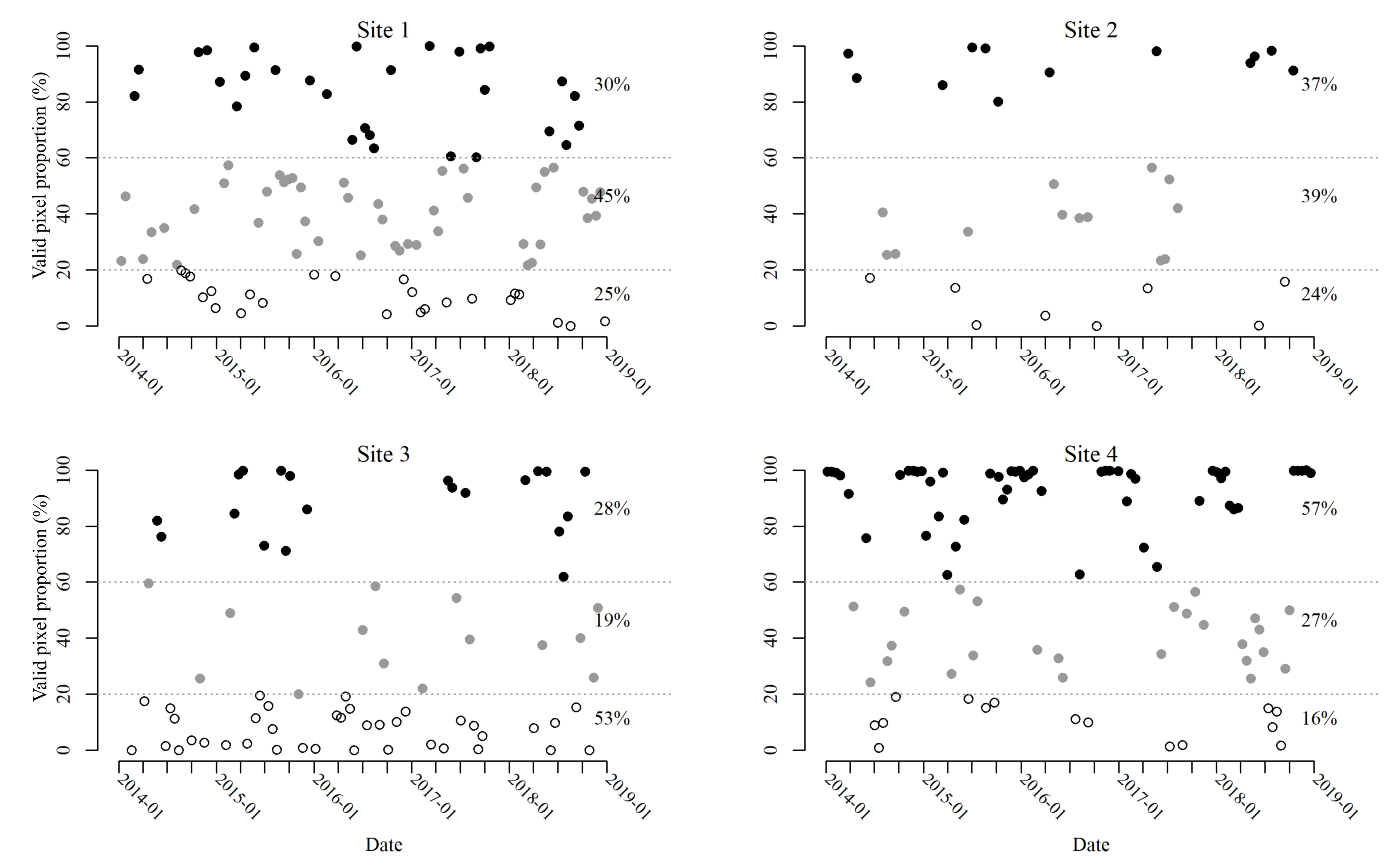
3.1. Study Area

We used the same four Landsat 8 sites as were used in developing MOPSTM, and each site was reorganized into 60 km × 60 km areas. The locations are in Taita Taveta County, Kenya (3 18 S, 38 30 E), Pirkanmaa province, Finland (61 30 N, 23 46 E), Brandenburg, Germany (52 00 N, 13 24 E), and the Qinghai-Tibet Plateau, China (28 40 N, 89 10 E) (Figure 1). The four sites feature various topographical and vegetation types, such as tropical montane forest in hilly areas and savannas in the plains in Site 1; boreal forests, croplands, and lakes in Site 2; broad-leaved forests and croplands in relatively flat terrain in Site 3; and high plains and mountains above the timberline in Site 4. The LULC types in the four sites are forest, bushland, grassland, cropland, built-up areas, and water.

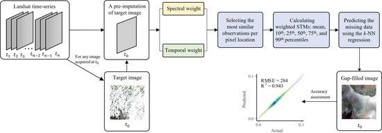
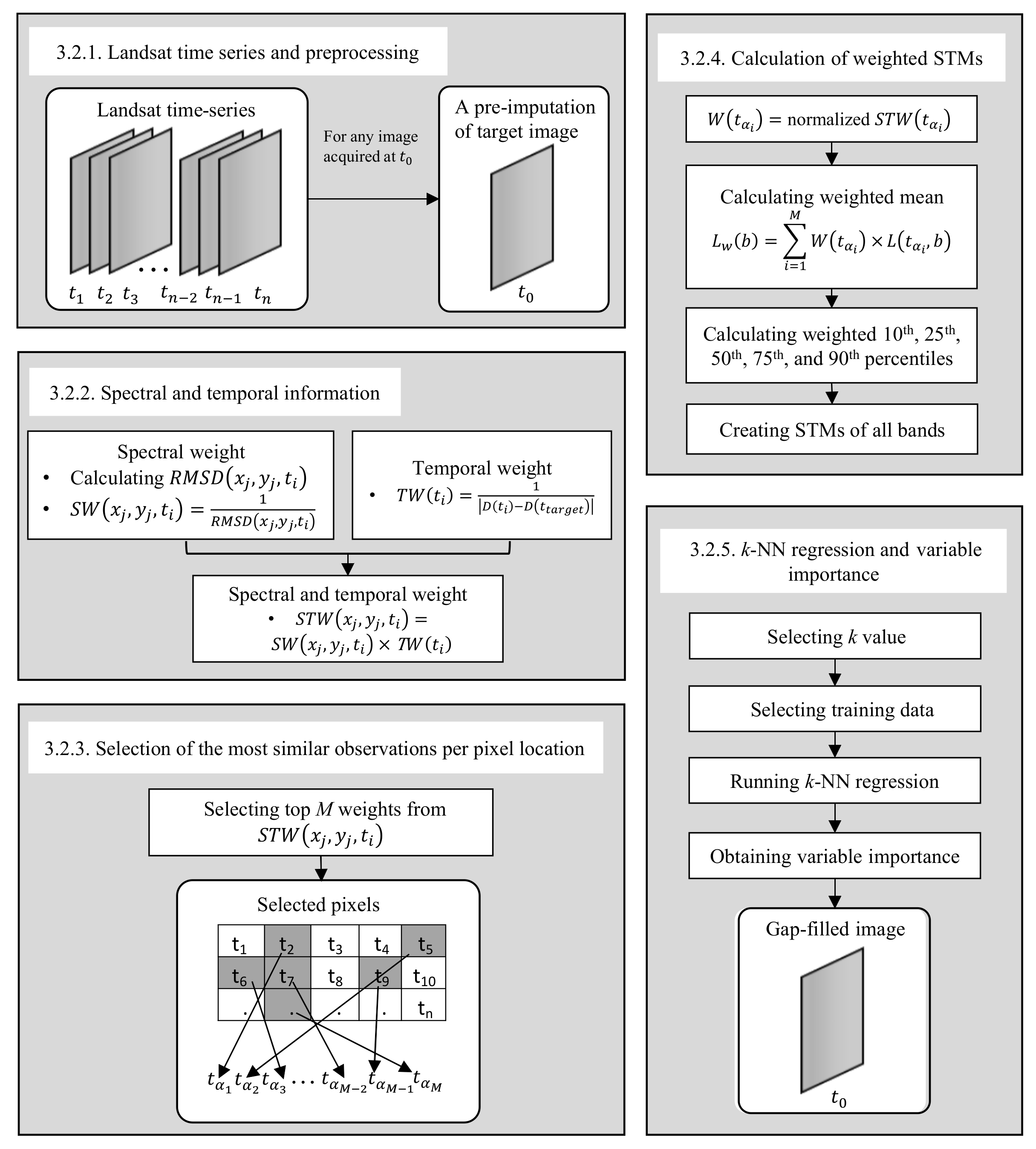
3.2. STIMDR Algorithm

A flowchart summarizing the STIMDR algorithm is shown in Figure 2. For convenience, we refer to an image having pixels that have been labeled as simulated gaps in the CCS mask as a “target image”. Here, we summarize the procedure of the main steps, and then, in the following sections, we explain them in greater detail. Before the gap-filling process, the Landsat time series is preprocessed, and a pre-imputation of the missing data in the target image is required because missing data cannot be used to calculate the spectral similarity between the target image and the other images. Here, the MOPSTM gap-filled images are used as the pre-imputation images.
The main steps in STIMDR are (i) to calculate the weight based on the spectral and temporal information, (ii) to find the most similar observations per pixel over the time series, (iii) to calculate weighted STMs including the weighted mean and weighted quantiles (10th, 25th, 50th, 75th, and 90th percentiles) with the spectral and temporal weights, and (iv) to train the k-NN regression using valid pixels in the target image and to predict missing values in the gaps. The overall procedure is repeated for each image in the time series.

3.2.1. Landsat Time Series and Preprocessing

We obtained Landsat 8 Operational Land Imager (OLI) Collection 1 Level-2 Surface Reflectance products from the USGS website https://earthexplorer.usgs.gov (accessed on 10 November 2021) the four sites (Table 2) and used seven spectral bands, including ultra blue, blue, green, red, near-infrared (NIR), and two shortwave infrared (SWIR1 and SWIR2) bands in each image. We reorganized the image size as 2000 × 2000 pixels for each site and obtained a long temporal period from the beginning of 2014 to the end of 2018. Images entirely covered by CCS were excluded, and thus the number of images collected over the 5-year period differed between sites. We performed the same preprocessing steps, e.g., removing pixels contaminated by CCS from CFMask cloud masks [53] and converting the reflectance to a range between 0 and 1 as was performed for the MOPSTM method [18]. At the end of this phase, we had the target image pre-imputed with temporary values (for missing data) that would be replaced with the final gap-filled values.
Images in the time series have different numbers of valid pixels (Figure 3). As 53% of the images in the time series had valid pixels under 20%, Site 3 had the poorest image quality. In contrast, as 57% of the images in the time series had valid pixels over 60%, Site 4 had the best image quality. As continuous CCS occurred (e.g., between September 2017 and March 2018), Site 2 had the fewest images in the time series.

3.2.2. Spectral and Temporal Information

For example, a consistent dense time series of Landsat images is a precondition for several remote sensing applications. A good time series is characterized by a temporal consistency, which is defined as data that were collected close in time having similar values [54,55]. Ideally, images acquired from the same geographic location in the time series should have similar values; however, natural and artificial disturbances, as well as phenological shifts (due to climate oscillation cycles), may alter the observations, and thus change the spectral values at the acquisition time. Therefore, we used the spectral and temporal information to measure the temporal consistency of the observations per pixel over the time series. We used the spectral similarity, generated from a root mean square deviation (RMSD):
R M S D ( x j , y j , t i ) = b = 1 B ( L ( x j , y j , t i , b ) L ( x j , y j , t t a r g e t , b ) ) 2 B
where L ( x j , y j , t i , b ) is the reflectance of the pixel located in ( x j , y j ) in the bth band of an image acquired from date t i , i starts from 1 and ends at the total number of pixels in a image, L ( x j , y j , t t a r g e t , b ) is the reflectance of the pixel located in ( x j , y j ) in the bth band of a target image acquired from date t t a r g e t , and B is the number of bands. A large RMSD value indicates a large spectral difference between the target image and the image in the time series. In other words, areas with high spectral difference, such as fields with agricultural crop rotation, will have large RMSD; other areas with low spectral variation, such as water or evergreen forest, will have small RMSD.
The spectral weight S W ( x j , y j , t i ) was computed as the reciprocal of R M S D ( x j , y j , t i ) , and it was pixel-based:
S W ( x j , y j , t i ) = 1 R M S D ( x j , y j , t i )
We used the temporal information derived from the acquisition dates between a target image and images in the time series. Therefore, the temporal weight transformed from that was image-based and expressed as:
T W ( t i ) = 1 | D ( t i ) D ( t t a r g e t ) |
where D ( t i ) denotes the image acquired on the date of t i , and D ( t t a r g e t ) denotes the date of the target image. The unit of the date difference is day.
As combining the individual strength of spatial and spectral domains can make better use of their hidden correlations [17], we combined S W ( x j , y j , t i ) and T W ( t i ) to obtain a new weight S T W ( x j , y j , t i ) (which is similar to a synthetic index based on the spectral similarity and geographic distance [13]):
S T W ( x j , y j , t i ) = S W ( x j , y j , t i ) × T W ( t i )
where S T W ( x j , y j , t i ) is the pixel-based spectral and temporal weight, meaning that every pixel in the time series has a value of S T W ( x j , y j , t i ) with respect to the pixel in the same location from the target image. Large values in S T W ( x j , y j , t i ) indicate high similarity of pixels in the time series and the target image, and small values indicate low similarity between these pixels.

3.2.3. Selection of the Most Similar Observations Per Pixel Location

Even preprocessed by the cloud removal algorithm [53], observations contaminated by cloud shadows remain present in the pixel location over the time series [56]. These observations, as well as the observations resulting from land surface changes at a time, usually have high heterogeneity (low similarity) to those in the target image, affecting the weighted spectral response [57,58] and potentially resulting in outliers greatly falling above or below the observations along the time series over the pixel values. To attenuate such phenomena, we used a threshold M to filter out the observations with high heterogeneity in each pixel location. In other words, observations with top M spectral and temporal weight S T W ( x j , y j , t i ) rankings are selected to derive the weighted STMs. Using a mapping in α : from N to N , where N is the set of positive integers less than or equal to the number of images in a time series, t α i is equal to the ith observation that is selected from the time series. Thus, the selected observations are denoted as ( x j , y j , t α 1 ) , ( x j , y j , t α 2 ) , ( x j , y j , t α 3 ) , , ( x j , y j , t α M ) .
A sensitivity test of M helped decide its proper value (Supplementary Table S1). Although a variety of M yielded the same accuracy in some cases, we chose the one that fell in the middle of the range. In this work, we used M = 20 in Site 1, M = 20 in Site 2, M = 11 in Site 3, and M = 5 in Site 4.

3.2.4. Calculation of Weighted STMs

The spectral and temporal weight S T W ( x j , y j , t α i ) was transformed as below:
W ( x j , y j , t α i ) = S T W ( x j , y j , t α i ) / i = 1 M S T W ( x j , y j , t α i )
The range of W ( x j , y j , t α i ) is between 0 and 1. A weighted mean matrix was calculated as:
L w ( x j , y j , b ) = i = 1 M ( W ( x j , y j , t α i ) × L ( x j , y j , t α i , b ) )
where L w ( b ) is the weighted mean reflectance in band b.
In addition to the weighted mean, we also applied the weights to the quantile estimation [59,60] and calculated the weighted quantiles (10th, 25th, 50th, 75th, and 90th percentiles) based on the quantile estimators [61], summarized as a median-unbiased estimator, independently of the underlying distribution. The weighted mean matrix and the weighted quantiles were stacked together as STMs (Supplementary Figure S1) [18], which were used as feature space in the k-NN regression described in the next section.

3.2.5. k-NN Regression and Variable Importance

We employed the k-NN regression to find the closest pixels in the feature space (STMs) to the missing pixel and thus predict the value. We used k-NN regression with KD Tree in the “FNN v1.1.3” package [62] of the R software environment [63]. Euclidean distance was employed in the calculation of distance as it was used in [18]. Before running k-NN models, we tuned the k values between 1 and 25 and then selected the optimal k value with respect to root mean square error (RMSE). The training and test datasets contained 10,000 pixels for each k tuning experiment. To assess how the variables in the weighted STMs performed when predicting gaps, we computed the variable importance using the R package “caret” [64] in the k-NN regression models.

3.3. Accuracy Assessment

3.3.1. Evaluation Metrics

The filled gaps were qualitatively evaluated by visually examining the spatial continuousness and the presence of noise. Evaluation metrics were also employed to assess the accuracy quantitatively. The agreement of the gap-filled and actual pixels was evaluated using RMSE and R 2 :
R M S E ( b ) = 1 N × i = 1 N ( L ( x j , y j , b ) L ^ ( x j , y j , b ) ) 2
R M S E ( x j , y j ) = 1 B × b = 1 B ( L ( x j , y j , b ) L ^ ( x j , y j , b ) ) 2
R 2 = 1 j = 1 N ( L ( x j , y j , b ) L ^ ( x j , y j , b ) ) 2 j = 1 N ( L ( x j , y j , b ) L ¯ ( b ) ) 2
where N is the total number of gap-filled pixels, L ( x j , y j , b ) and L ^ ( x j , y j , b ) are the actual and predicted values, respectively, of the ith pixel in bth band, and L ¯ ( b ) is the mean value of L ( x j , y j , b ) in the bth band.

3.3.2. Performance Comparison with Existing Methods

We compared our method, STIMDR, with four hybrid methods (WR, gapfill, SAMSTS, and MOPSTM methods) and three temporal interpolation methods (a non-rounded Akima spline, Steffen spline, and OTB spline methods). The performance of SAMSTS and MOPSTM has been compared in the previous work [18].
The parameters in the WR method were set as follows: The spatial radius r equals 20, the temporal radius t equals 3, and the minimum pairings m equals 3. A large radius enables missing pixels that are far away from the valid pixels in spatial distance to be recovered. To speed up the performance, we divided the target image into 4 × 4 pieces.
The gapfill method is open-source and can be performed in parallel computation. The parameters for the gapfill method were set to default. To speed up the computation of gapfill, the target image was divided into 10 × 10 pieces, processing with multiple CPU cores. Since WR and gapfill cannot fill all the gaps in the four Sites, we compared the overall accuracy in the common regions that were reconstructed by them.
SAMSTS is an open-source algorithm, the parameters of which were set to default defined in the coding document [65]. As MOPSTM was not computation-demanding, we trained the target image at its full size.
The temporal interpolation methods did not have large computing time cost, so they were implemented on the full-size images, processed with multiple CPU cores. Akima spline interpolation requires a minimum of five points in time series, so we removed the pixels that had fewer than six valid points in the pixel location throughout the period.
For OTB gap-filling, we chose the “spline” instead of “linear” method as the 5-year time series met the requirement of more than five valid dates in most of the areas [39]. However, with fewer than three valid dates, it would apply linear interpolation, while with three or four valid dates, cubic splines with natural boundary conditions would be used.
To better summarize how the STIMDR results have improved over MOPSTM, we compared the histogram of absolute residuals and the median absolute deviation (MAD) [66,67] of these two methods. The absolute values of residuals are the absolute difference between the filled values and the actual values in each band; MAD is defined as the median of the absolute deviations from the median of the data and is a robust estimator of dispersion, better at highlighting differences in non-parametric data distribution.
Furthermore, we tested if the residual populations were significantly different using the Wilcoxon rank sum test, which has been frequently used in statistical practice for the comparison of skewed data distribution [68,69]. The absolute pixel values of residuals from the common areas reconstructed by all the methods were compared in this test.

3.3.3. Experiments of Filling Single-Date Images

For filling single-date images, four nearly cloud-free target images from Sites 1–4 were acquired from 9 March 2017, 21 August 2015, 12 October 2018, and 10 December 2014, respectively. After simulating gaps, valid pixel percentages were 37.3% (Site 1), 39.3% (Site 2), 15.3% (Site 3), and 26.4% (Site 4). Training datasets contain 30% of the valid data selected using systematic sampling from the overall valid pixels. As the test datasets were simulated gaps, there was no overlap between the training and test datasets. The referenced pixels in gap locations were used to evaluate the k-NN prediction. To obtain stable accuracy, we repeated the experiments 10 times using different training datasets (30% of the overall valid pixels).
(i) Overall accuracy using the evaluation metrics
We assessed the overall gap-filling performance using RMSE and R 2 that were calculated from the actual values and filled values using different methods.
(ii) Dependence of the number of the observations
As the number of the observations per pixel location throughout time series can be a driver behind overall RMSE, we examined how the RMSE relies on the number of observations using different gap-filling methods. The pixels were from the common regions that have been filled by these methods.
(iii) Accuracy for spectral bands
To evaluate the accuracy for different spectral bands, we calculated the linear regression between the filled values and actual values for every single spectral band.
(iv) Accuracy for LULC types
To assess the algorithms’ performance on different LULC types, we evaluated RMSE for the different methods over six LULC types, including forest, bushland, grassland, cropland, built-up areas, and water. The reference data were the same datasets that were used in the previous studies [18].
To examine the accuracy variation of STIMDR with respect to its sensitivity to LULC type imbalance, we demonstrated RMSE for six LULC types given that one specific LULC type was missing in the training datasets. We randomly selected 1000 pixels from every LULC type, and thus there were a total of 6000 pixels. The 10-fold cross-validation was applied to the datasets. We eliminated pixels from one specific LULC type in the training datasets while predicting the test datasets which had pixels from all LULC types. The specific missing type is from the six LULC types in order. To obtain stable accuracy, we repeated the experiments 10 times.

3.3.4. Experiments of Filling Images in Time Series

For filling time-series images, gap pixels were simulated by allocating a random sampling method to valid pixels. Various random 10,000-pixel masks were applied to each image to create artificial gaps before they were reconstructed by different gap-filling methods. To obtain comparable results, all gap-filling methods filled the same pixels in one image while the distributions of the gap pixels were random per image. As WR and gapfill cannot fill all the gaps in the four Sites, they were not included in the time-series experiments. Moreover, we did not include SAMSTS because of its lack of support for parallel operations. For MOPSTM and STIMDR, the training datasets were both 100,000 pixels. Images that had a valid pixel number less than 100,000 were removed.

3.3.5. Experiments of Gap-Filled Images for LULC Classification Applications

To evaluate how the gap-filled images perform with respect to remote sensing applications, we generated LULC products derived from the single-date gap-filled images reconstructed by all the methods and compared them with those generated from the original images.
We used Random forest classifier [41,70,71] with training datasets derived from 5% of all the pixels in seven bands in the gap-filled and original images by stratified sampling. The training datasets were from the same location and identical in number for each gap-filled and original image in each site; the test datasets were all the gap pixels. The number of test datasets was about 1.22 million, 2.41 million, 3.37 million, and 2.93 million in Sites 1–4, respectively. In each site, different methods had slightly different numbers of the gap-filled pixels because a few pixels might remain unfilled. For example, Akima and Steffen methods did not fill any pixel location that had less than six valid observations over the 5-year period. Accordingly, test datasets of the original images were from the locations where artificial gaps were created. To compare accuracy between actual and gap-filled datasets, the classification results were evaluated using producer’s accuracy, user’s accuracy and overall accuracy [13,72].
It is worth noting that the goal of the LULC classification experiment was not to generate the best LULC classification products, which can be generally done using more sophisticated classifiers employed with multiple dates of imagery, ancillary sources of data, and high-quality LULC reference data [13]. Instead, our goal was to compare between our method, other gap-filling methods, and real observations, thereby giving us an insight on how gap-filled images using our method are applicable to remote sensing applications.

4. Results

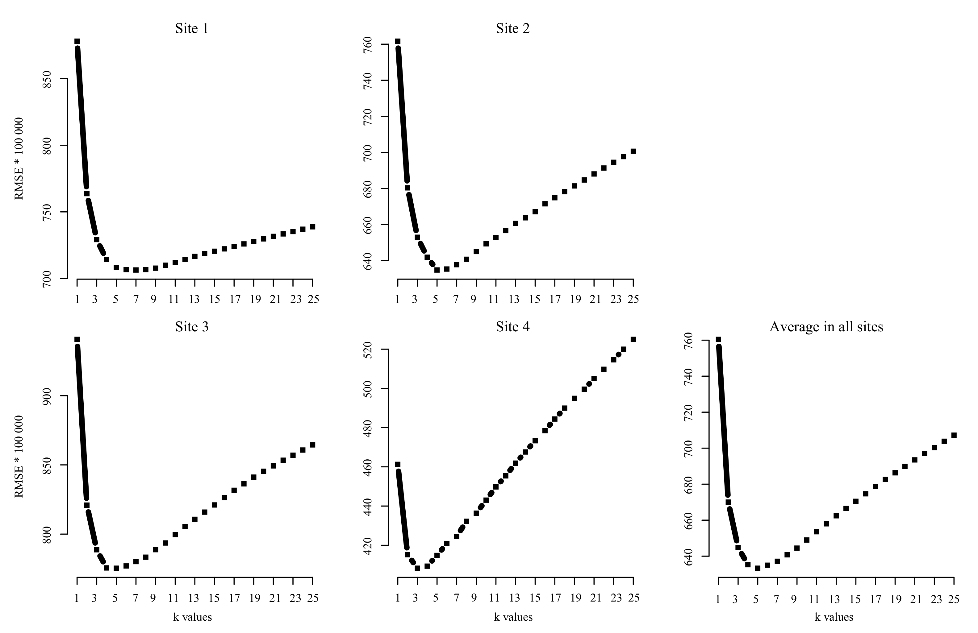
4.1. Optimization of the k Value and Importance of Variables

RMSE (multipled by 100,000) with respect to the k value ranging from 1 to 25 is shown in Figure 4. All sites had a strict convex shape of RMSE with an increase in k value. Thus, the curves showed a steep decrease when k started from one to three and reached the bottom of a trough before rising. The best k values, corresponding to the minima in RMSE, were 7, 5, 5, and 3 for Sites 1–4, respectively. Based on all four sites, the average RMSE was minimized when k was five.
Forty-two variables (e.g., Site 1 in Supplementary Figure S1) were tested for gap filling in all sites. The 10 most important variables are shown in Supplementary Figure S2 according to their importance score. A high score represents high importance, and the most important variables have a score of 100. We found that variable importance differed at every band. For example, the most important variables for the blue band were itself, green, ultra blue, and red bands, and the most important variables for the NIR band were itself, red, and SWIR bands.

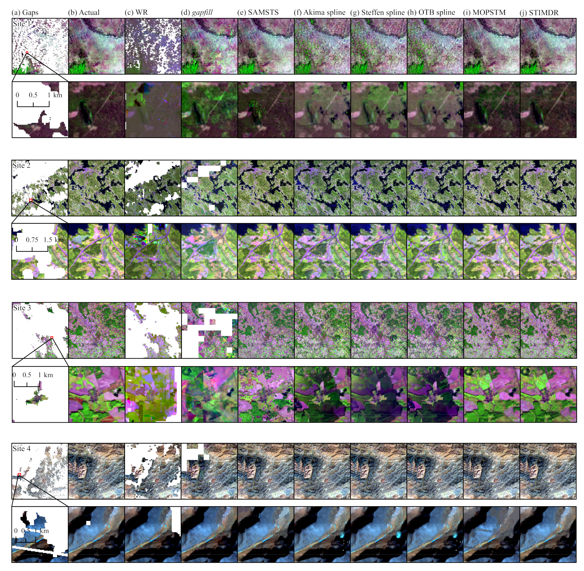
4.2. Results for Filling Single-Date Images

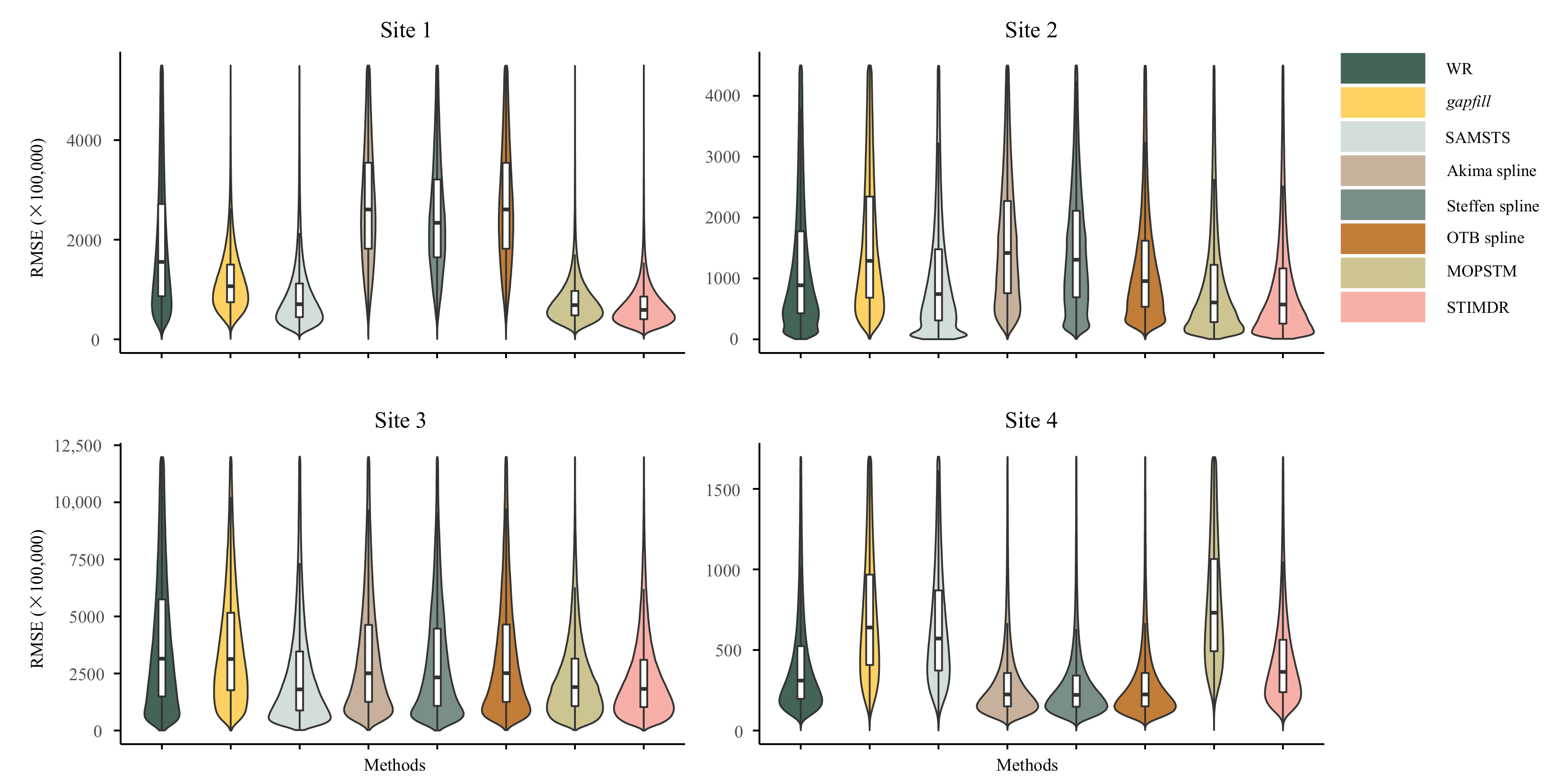
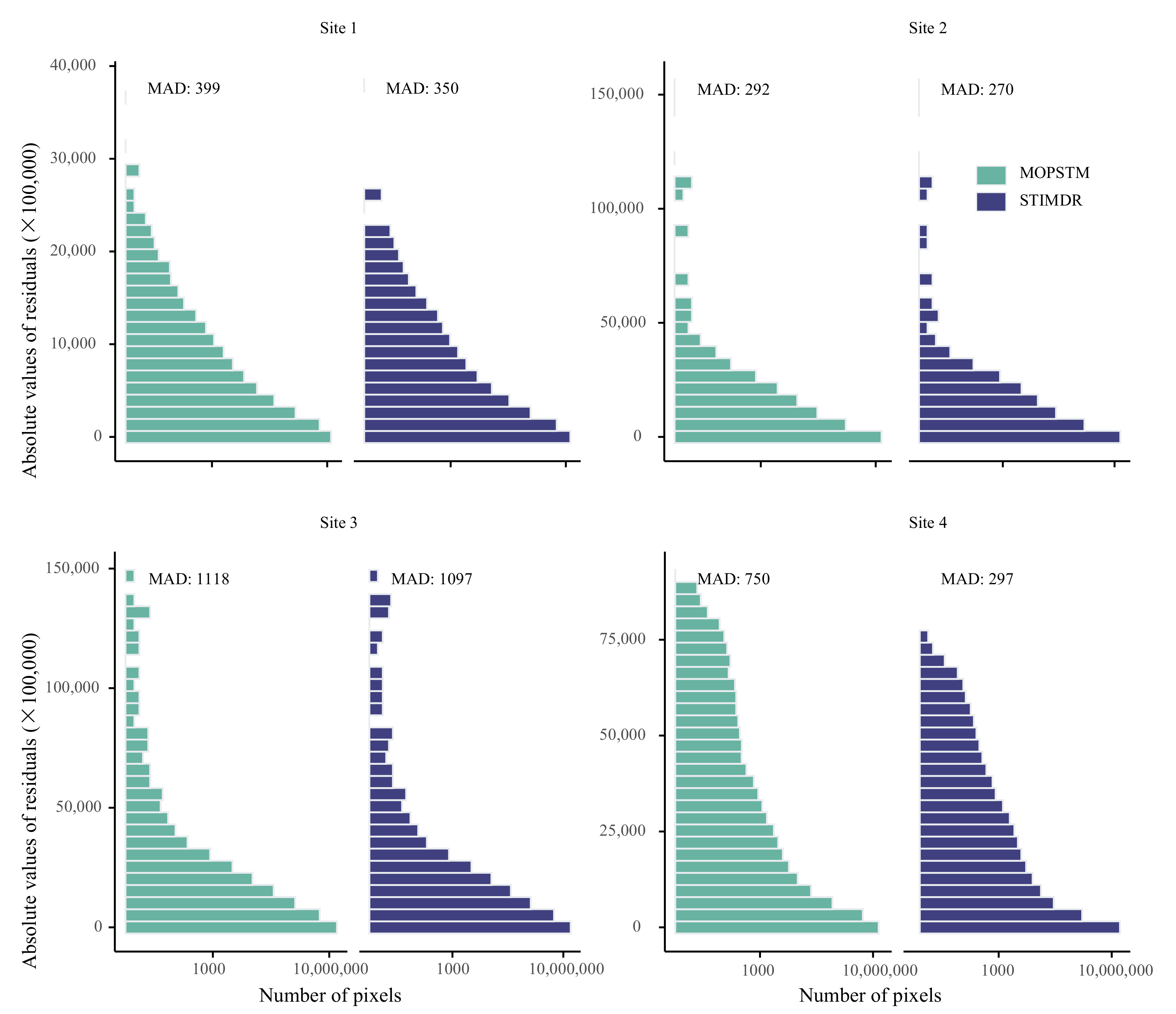
4.2.1. Overall Accuracy

Eight gap-filled results are compared in Figure 5, and their pixel-based RMSE values are displayed in Supplementary Figure S3. In general, STIMDR produced the smoothest and most natural-looking reconstructed images. MOPSTM was the second best on average, although it produced artifacts when recovering stripe-shaped gaps for Site 4. SAMSTS performed better than all methods other than MOPSTM and STIMDR but rendered noisy pixels (e.g., in Site 3). The three temporal interpolation methods produced similar results. WR and gapfill could not recover all the gaps, especially the large-area gaps. gapfill only recovered all the gaps for Site 1, and it performed more accurately than WR and the temporal interpolation methods. WR was the worst, only recovering adjacent pixels around the valid pixels but producing extreme large or small values.
In terms of the common regions that had been constructed by all the methods, STIMDR yielded smaller RMSE and larger R 2 values, e.g., (mean values of 10 repeated experiments with different training datasets) than any other method on average (Figure 6 and the “Partial” columns in Table 3). MOPSTM was the second best on average even though it had the lowest accuracy for Site 4. WR delivered the lowest accuracy, which was far worse than the accuracy of any other method (except for Site 4), e.g., gapfill succeeded in reconstructing all the gaps only in Site 1, so it has the “Full” result for Site 1 only. For Sites 1–2, gapfill performed better than temporal interpolation methods, but worse than them for Sites 3–4. SAMSTS had smaller RMSE than other methods except for MOPSTM and STIMDR and had the smallest mean RMSE for Site 3 (Figure 6). The OTB spline yielded very similar accuracy to the Akima spline but was better for Site 2. The Akima and OTB splines outperformed STIMDR for Site 4 because the interannual features of the land surface changed slowly, and cloud cover was less frequent during the studied years in high-altitude areas in Site 4.
For methods that were able to fill all the gaps, there was a slight difference between the full and partial accuracy (Table 3), except for Site 4, where the partial RMSE was approximately only half the full RMSE for most of the methods.
In addition to RMSE and R 2 , the histogram of absolute residuals and MAD indicated a relatively clear improvement between MOPSTM and STIMDR (Figure 7). In Figure 7, MOPSTM predicted more pixels that had extremely large absolute residuals, especially in Site 4. The difference in MAD is larger than 20 between these two methods in all sites.
For example, the Wilcoxon rank sum test (Supplementary Tables S2–S5) confirmed that distributions were mostly significantly different (p < 0.05). Only the Akima spline and the OTB spline methods were not significantly different for Site 1 (p-value 0.29) and Site 4 (p-value 0.78).

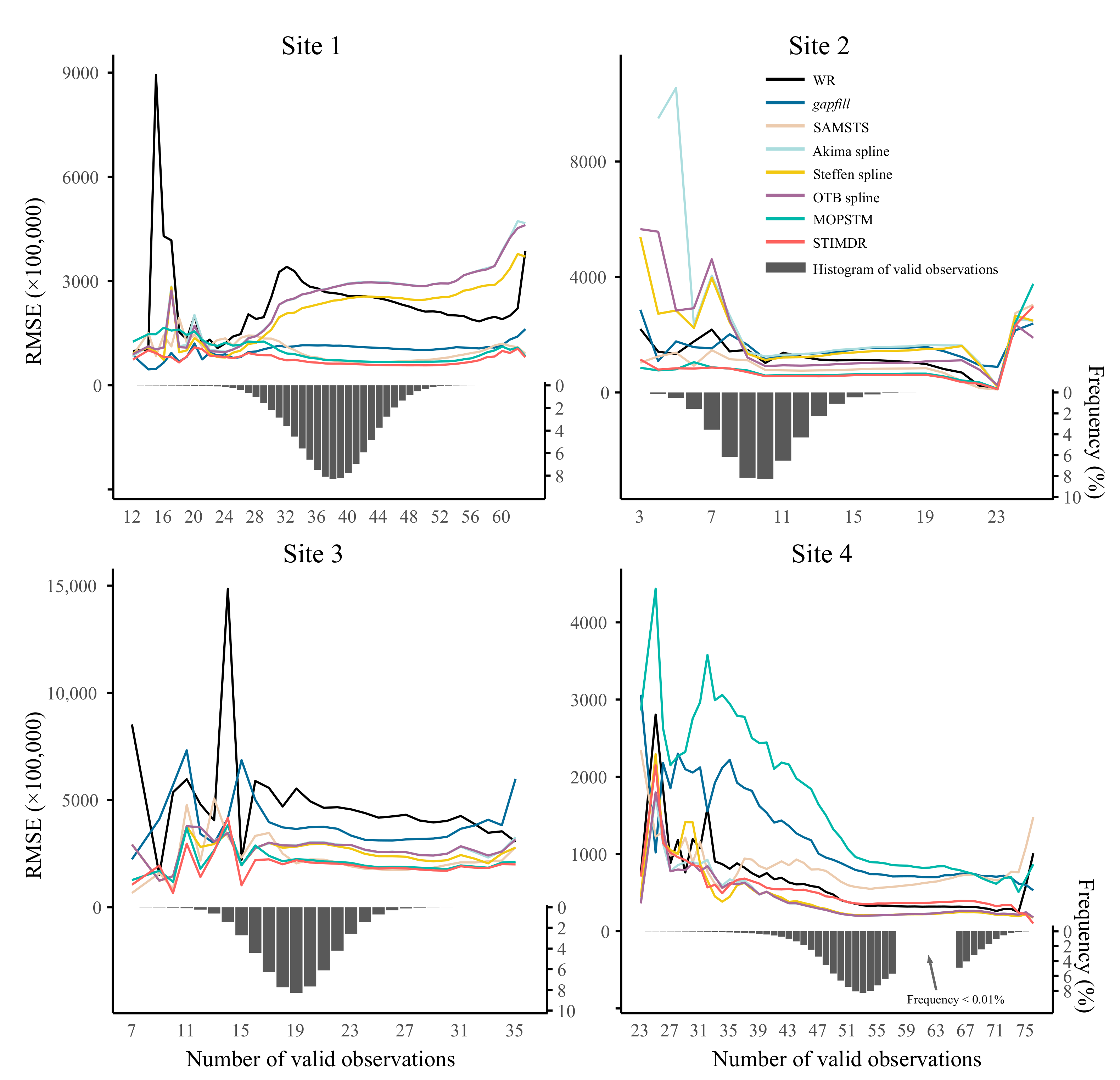
4.2.2. Dependence of the Number of the Observations

We demonstrate the dependence of the median RMSE of the methods on the number of observations per pixel location throughout the 5-year period in Figure 8. In general, the trend indicates a drop in RMSE with an increase in the valid observations in the time series, such as in Site 2 and Site 4. STIMDR was the least affected by the number of valid observations in the time series, and it delivered robust performance on pixels that had an extremely small number of valid observations throughout the time series. WR had the greatest fluctuation by the valid observations on average, e.g., in Site 1 and Site 3.

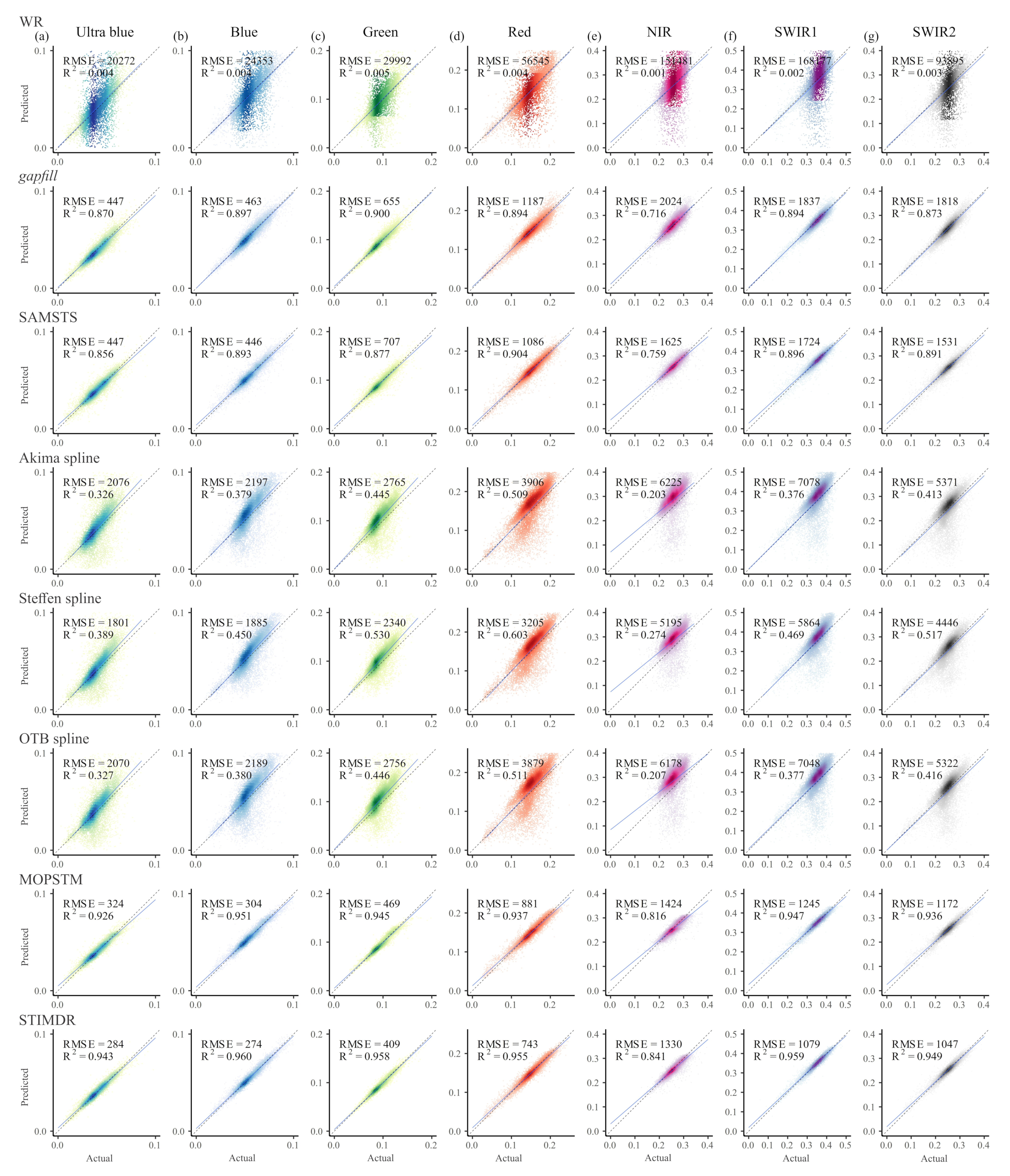
4.2.3. Results for Spectral Bands

Scatter plots (Site 1 in Figure 9 and Sites 2–4 in Supplementary Figures S4–S6) show the relationships between the referenced values and the gap-filled values from the common regions using the eight methods for seven spectral bands. WR had the largest error, resulting in an extremely small R 2 . Temporal interpolation methods had biased fitted lines between actual and predicted pixels with most of the R 2 less than 0.60. SAMSTS was slightly better than gapfill on average. Both MOPSTM-filled and STIMDR-filled pixels were closer to the 1:1 line than the other methods, indicating their superior performance in each spectral band. The ranking of the eight methods from the most to the least accurate is STIMDR > MOPSTM > SAMSTS > gapfill > Steffen spline > OTB spline ≥ Akima spline > WR.

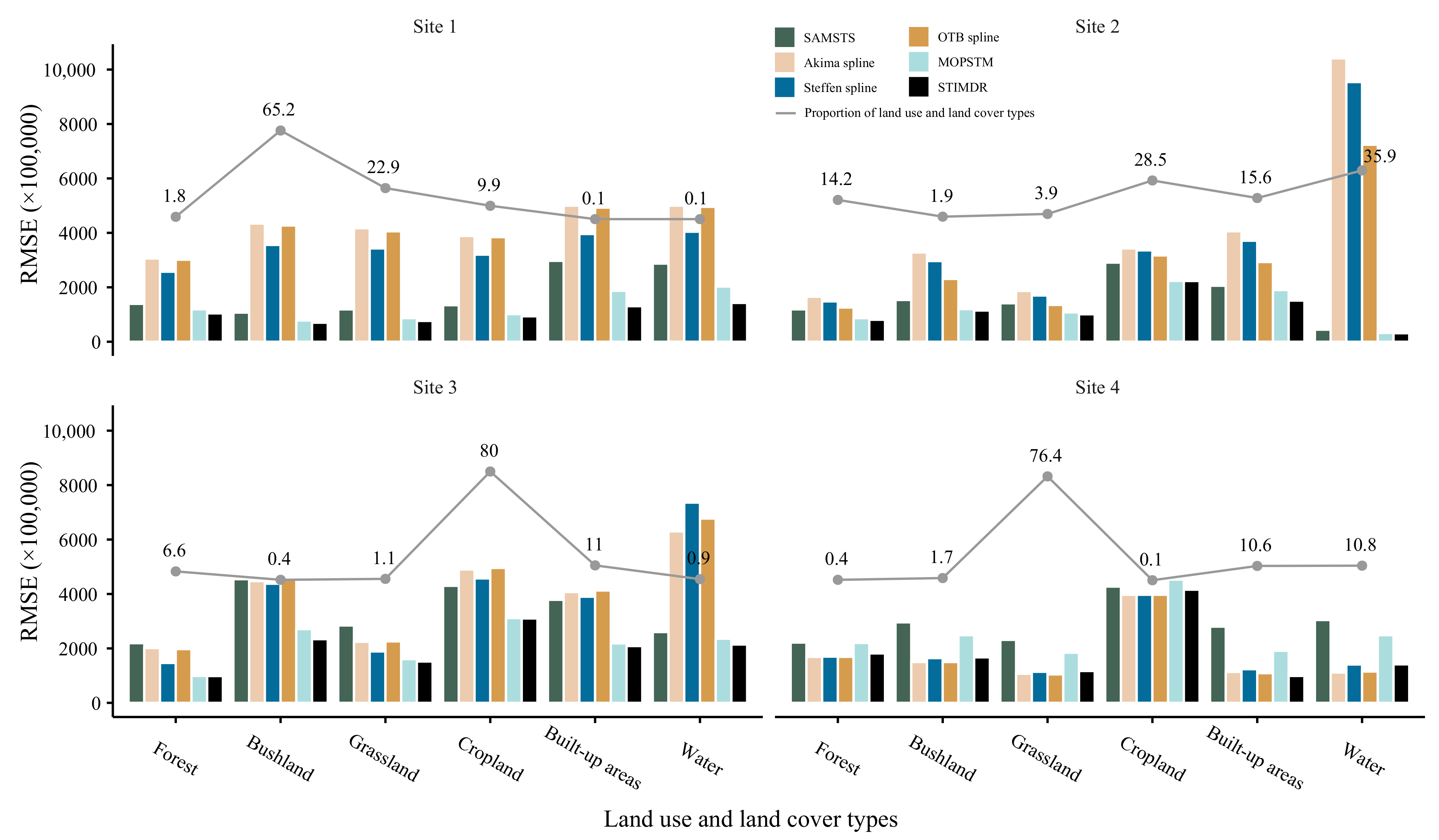
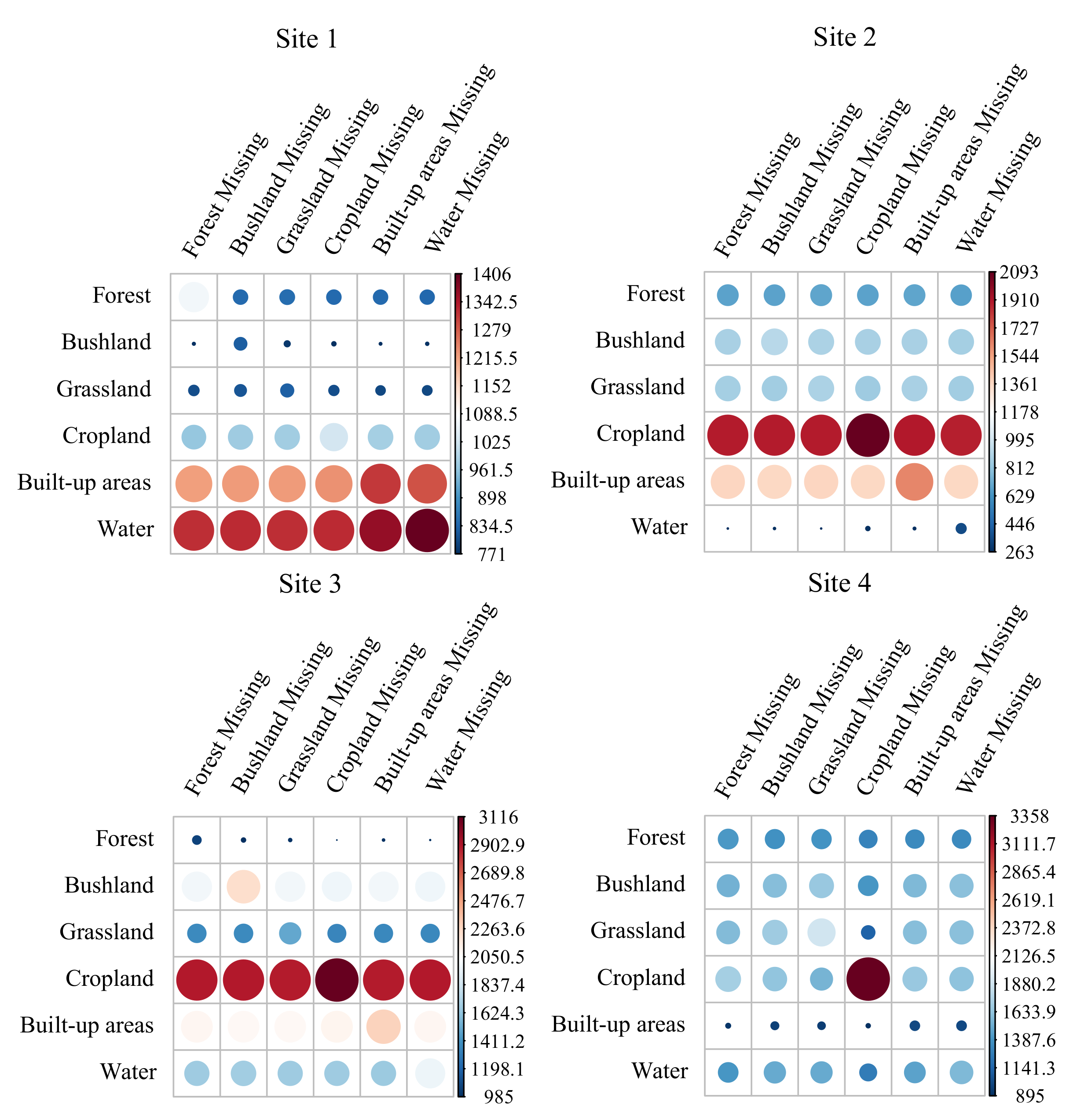
4.2.4. Results for LULC Types

Figure 10 demonstrates RMSE for six LULC types in four sites. Consistent with the overall RMSE (Table 3), STIMDR had the highest accuracy for most of the LULC-specific situations. The greatest difference between the performance of STIMDR and the temporal interpolation methods was observed at the water type in Site 4. The overall ranking for the six methods from the most to the least accurate in terms of LULC accuracy is STIMDR > MOPSTM > SAMSTS > Steffen spline > OTB spline ≥ Akima spline.
In terms of sensitivity to LULC type imbalance (Figure 11), STIMDR did not show a clear drop in RMSE of a specific LULC type when this LULC type was missing in the training datasets. For example, the grassland type in Site 1 yielded almost the similar RMSE no matter which LULC type was missing in the training datasets. It should be noted that some types were sensitive to the absent proportion of pixels from their own types in the training datasets. Such types are forest in Site 1, bushland in Site 3, and cropland in Sites 2 to 4.

4.3. Results for Filling Images in Time Series

RMSE for reconstructed Landsat 8 time series is demonstrated in Figure 12. The numbers of the images evaluated were 95, 32, 68, and 91 for Sites 1–4, respectively. With respect to the average RMSE of the five methods, STIMDR was always the smallest (2966, 2105, 3206, and 3298 for Sites 1–4, respectively) while the OTB spline was always the highest (4928, 10,465, 8697, and 8477 for Sites 1–4, respectively). In addition to considerable improvement in accuracy, STIMDR showed high overall robustness as it had very few outliers (relatively high RMSE values), which occurred many times using the OTB spline method.

4.4. Results of Gap-Filled Images for LULC Classification Applications

For example, Table 4 demonstrates the LULC classification results for all Sites. Compared with the gap-filled images using other methods (Table 4), STIMDR-filled images had the closest overall accuracy to the original images for producing classification products and even surpassed the original images (74.3%) in overall accuracy in Site 2 (74.9%). This supports the assertion that STIMDR results can be used in LULC mapping applications. In addition to STIMDR, MOPSTM also showed similar classification results to the original images.

5. Discussion

The ability to produce gap-free Landsat time series in a simple and efficient way can significantly improve remote-sensing applications for land-surface characterization, analysis, and monitoring [1]. Although there are several image reconstruction methods proposed to fill Landsat 7 SLC-off [73] and CCS gaps [74,75], methods that are simple to tune on a global scale, fast in computation, and robust in producing a time series of gap-free imagery are still scant [76,77]. The newly published method, Missing Observation Prediction based on Spectral-Temporal Metrics (MOPSTM), has demonstrated high performance in predicting large-area gaps with respect to spatially heterogeneous land-cover areas and has the potential to generate gap-free Landsat time series [18]. However, it is limited to deriving STMs for a fixed period (e.g., one year), thus restricting its performance by ignoring useful spectral and temporal information beyond the fixed period. Moreover, MOPSTM is unable to fill gaps in extreme circumstances where local areas are entirely covered by successive CCS during the 1-year period. Therefore, we propose a new method, STIMDR, to overcome the limitations of MOPSTM and produce gap-free images in a longer time series by employing spectral and temporal information to select similar observations per pixel location.

5.1. Comparisons with the Other Gap-Filling Methods

STIMDR was compared with three temporal interpolation methods (Akima spline, Steffen spline, and OTB spline) and four other hybrid methods (WR, gapfill, SAMSTS, and MOPSTM), each of which has been commonly used in remote sensing applications [28,33,36]. STIMDR held overwhelming advantages over these methods in visual accuracy assessment between gap-filled images versus actual images in terms of visual analysis (Figure 5), pixel-based RMSE (Supplementary Figure S3), quantiles of pixel-based RMSE (Figure 6), median RMSE dependent on the number of valid observations (Figure 8), quantitative evaluation of spectral bands (Figure 9) and LULC types (Figure 10), and a down-stream task of LULC classification (Table 4). The overall ranking of the eight methods from the most to the least accurate is STIMDR > MOPSTM > SAMSTS > gapfill > Steffen spline > OTB spline ≥ Akima spline > WR.
Reliant on the size of the spatial neighborhood, WR failed to recover all the gaps, especially those that covered a large area. gapfill can recover pixels that have a long distance to the valid pixels, but can fail in filling gaps of an enormous spatial size. The disadvantages of the temporal interpolation methods are rather distinct, one important pitfall of which is overfitting [78]. In addition, making no use of spatial information resulted in obvious artifacts at the junctions (e.g., Site 1 in Figure 5f–h). Potential issues of temporal interpolation methods that could affect the accuracy are the length of the temporal interval of the missing values, the number of existing valid pixels, and whether the cloud-contaminated pixels exist among the valid pixels. For example, the Akima and Steffen spline methods had the largest RMSE for Site 2, where the fewest valid pixels were collected among the four sites over the period. WR and the temporal interpolation methods tended to have good performance when sufficient valid observations existed in the time series (e.g., Site 4). Superior to WR, gapfill, and the temporal interpolation methods, SAMSTS delivered higher accuracy but produced unwanted noise, likely due to the segmentation process [18]. MOPSTM performed more accurately for Sites 1–3 than all methods other than STIMDR, but performed the least accurately for Site 4. STIMDR was the greatest improvement over MOPSTM in Site 4, which proved the positive effects of using spectral and temporal weights. Moreover, STIMDR is capable of predicting smooth values at the junctions, which likely benefits from employing k nearest pixels in the spatial neighborhood.
Generating and employing weights enable more important observations to be emphasized [79,80,81]. Employing weights can be an effective way to improve performance [82,83,84]. The weights in STIMDR contain spectral and temporal information, which measures the temporal consistency per pixel over the time series. Observations with low temporal consistency often have small weights and thus have little impact on the weighted STMs. For example, pixels that undergo large LULC changes are more likely to have very small spectral similarity and a very large temporal distance given that large LULC changes are not typically observed over a short period [50]. Reducing the effects of the low-temporal-consistency observations helps improve the quality of STMs.

5.2. Computational Efficiency

The computations of WR, gapfill, MOPSTM and STIMDR were performed as parallel jobs using a single node in the Puhti supercomputer of CSC—IT Center for Science Ltd., Finland, equipped with 50 GB RAM in total and an Intel® Xeon® Gold 6230 processor with seven physical cores at 2.10 GHz base frequency. For filling the single-date images in a partial size, WR took about 10 h on average for an image size of 500 × 500 pixels using 1344 physical cores and 1.2 GB RAM for each core. gapfill ran over 20 h (maximum 40.5 h) on average for a image size of 200 × 200 pixels, consuming 8400 physical cores and 3 GB RAM for each core, making it the computationally heaviest (Table 5). For the experiment of gap-filling single-date images in a full size (2000 × 2000 pixels), the processing time of MOPSTM and STIMDR were about 1.8 and 2 h (without accounting for MOPSTM-imputation processing time) on average per image with seven bands, consuming 7 and 112 physical cores and approximately 40 GB RAM, respectively. The computation of the OTB spline in the Puhti supercomputer equipped with 2.5 GB RAM per core and 6 physical cores took about 0.6 h on average for the same experiment. The computations of the Akima and Steffen spline methods were conducted as parallel jobs on Yale University’s Grace cluster of 80 IBM NeXtScale nx360 M4 servers, using 7 E5-2660_v3 cores and about 2.8 GB RAM per core. For the same experiment, the Akima and Steffen spline methods took about 0.5 h each. SAMSTS was running on an Intel Core i5-7200 CPU at 2.50 GHz processor, 1 CUP core, 15 GB RAM, and took about 8 h. It should be noted that different programming languages are of different efficiency in running the same program.

5.3. Optimizing the User-Defined Parameters in a Global Implementation

In terms of implementing the proposed method globally, e.g., we recommend the performance of STIMDR in the High-performance-Computing environment where multiple cores are involved. We also recommend the same preprocessing steps that were performed in this work. The implementation of gap-filling can be mainly three steps: (i) calculating the pre-imputation of a target image using an accurate method (e.g., MOPSTM), (ii) calculating the spectral and temporal weights, and (iii) training and predicting in the k-NN regression. Although there are only a few parameters in STIMDR, tuning the optimal parameters is an unsolved problem, which is common in global implementation applications [85].
There are two parameters: (i) M, which selects the number of similar observations in the pixel location over the time series, and (ii) k values in the k-NN regression. Tuning M is challenging as different sites may have different optimal M. For example, the optimal M was around 20 for Site 2, while it was only 5 for Site 4. It seems that the sites with less vegetation tend to have a small M because the land surface is quite temporally stable. Sites located in cloud-prone areas are supposed to have large M so that more pixels will be included to derive STMs, e.g., the baseline is that M should be large enough to include at least an annual cycle of observations.
In this work, the k values in the k-NN regression were decided per site according to Figure 4, and thus k values can differ per site. Although a prior k value is challenging to define because training datasets can vary greatly from site to site, it is possible to predefine k values ranging from five to eight as a compromise before testing the method for other datasets. This was based on the fact that five was the optimal value to minimize the average RMSE for the four sites. A separate k tuning process is recommended when STIMDR is applied on a global scale. Other options, such as the weighted k-NN [86] that enables automatic k tuning in R package “kknn” [87], can be considered to replace the unweighted k-NN regression.

5.4. Limitations and Future Work

The minor disadvantage of STIMDR is that a pre-imputation of missing values in target images is required to calculate the spectral and temporal weights. However, it is not a problem if the pre-imputation of missing values is not available, as mean and median composites can be alternatives to imputing missing pixels in target images [88,89]. Furthermore, any other gap-filled products or a different source image acquired from a close date to the target image can be alternatives to the pre-imputation images.
Another limitation of STIMDR is that it can be biased to predict the missing values when the valid pixels are of a poor quality (e.g., a part of contaminated pixels remaining) or the lack of LULC types that are sensitive to seasonal variations (e.g., crop types). For example, STIMDR may have poor performance in filling cropland pixels if no cropland data can be collected in the training data (Figure 11). However, there are useful ways to avoid this extreme situation, e.g., extending the geographic extent of the target images to include sufficient pixels from the missing LULC type [18].
The performance of STIMDR is related to the quality of the weighted STMs. STMs derived from biased time-series data where information for an individual season is missing can affect the prediction of STIMDR using the k-NN regression.
In principle, STIMDR is applicable to other similar time series (e.g., Sentinel-2), and this should be tested in future studies. Here, the method was a better alternative to WR, gapfill, Akima spline, Steffen spline, OTB spling, SAMSTS, and MOPSTM and has the potential to be combined with other methods (e.g., image compositing, temporal smoothing, and model fitting) [18,49]. Future work can also focus on comparisons between gap-filling methods with image blending (fusion) techniques.

6. Conclusions

We propose a new gap-filling method, STIMDR, and demonstrated its potential to produce gap-free Landsat time series. The greatest advantage of the improved method is that it offers a flexible and effective way to derive target-image specific spectral-temporal metrics based on weights considering both spectral and temporal information. With STMs being the feature space, the k-NN regression machine-learning method was applied to train and predict missing values by setting identical model parameter and size of training and testing datasets per study site. STIMDR outperformed three spline interpolation methods (Akima spline, Steffen spline, and OTB spline) and four hybrid methods (WR, gapfill, SAMSTS, and MOPSTM) on Landsat 8 images of four sites with different land covers and topographies from 2014 to 2018. The results indicated its high performance in recovering heterogeneously vegetated areas such as tropical forests, broad-leaved forests in Europe, and high plateau vegetation in China. In follow-up studies, this method could be used to analyze the time-series features of remote sensing images, such as forest attributes and rangeland characterizations.

Supplementary Materials

The following are available online at https://www.mdpi.com/article/10.3390/rs14010172/s1, Figure S1: The weighted spectral-temporal metrics (STMs) for one target image in Site 1 acquired on 9 March 2017, displayed in false color of R: SWIR1, G: NIR, and B: red. W10th denotes weighted 10th, W25th denotes weighted 25th, W50th denotes weighted 50th, W75th denotes weighted 75th, W90th denotes weighted 90th percentiles and WM denotes weighted mean, Figure S2. Ten most important variables in the k-NN regression model. There were 10,000 training and testing pixels from target images. The horizontal axis denotes the importance scores, and the vertical axis denotes the ten most important variables containing weighted mean (WM), and weighted 10th, 25th, 50th, 75th, and 90th percentiles, Figure S3. Pixel-based RMSE (multiplied by 100,000) of gap-filled images using different methods (corresponding to Figure 5 in the four sites, displayed in false color of R: SWIR1, G: NIR and B: red surface reflectance. (a) window regression (WR), (b) gapfill, (c) SAMSTS, (d) Akima spline, (e) Steffen spline, (f) OTB spline, (g) MOPSTM, and (h) STIMDR. Each image size is 2000 × 2000 30 m pixels, resulting in 60 × 60 km. The valid pixel percentages were 37.3 (Site 1), 39.3% (Site 2), 15.3% (Site 3), and 26.4% (Site 4). Only gap pixels that have reconstructed are displayed, and the gap pixels that failed to be constructed are displayed in the black regions. Figure S4. Density scatter plot of window regression (WR), gapfill, SAMSTS, Akima spline, Steffen spline, OTB spline, MOPSTM, and STIMDR predicted values (y-axis) and validation values (x-axis) for seven spectral bands in Site 2. The black dashed line is the 1:1 line and the solid blue lines show the linear regression fits. Darker color shading: regions with a large density of points; lighter color shading: regions with a small density of points. RMSE was multiplied by 100,000. Figure S5. Density scatter plot of window regression (WR), gapfill, SAMSTS, Akima spline, Steffen spline, OTB spline, MOPSTM, and STIMDR predicted values (y-axis) and validation values (x-axis) for seven spectral bands in Site 3. RMSE was multiplied by 100,000. Figure S6. Density scatter plot of window regression (WR), gapfill, SAMSTS, Akima spline, Steffen spline, OTB spline, MOPSTM, and STIMDR predicted values (y-axis) and validation values (x-axis) for seven spectral bands in Site 4. RMSE was multiplied by 100,000, Table S1. The sensitivity of threshold M with respect to the root-mean-square error (RMSE), multiplied by 100,000.Table S2. Pairwise comparisons for Site 1 using Wilcoxon rank sum test where p-value larger than 0.05 are labeled in bold. Table S3. Pairwise comparisons for Site 2 using Wilcoxon rank sum test where p-value larger than 0.05 are labeled in bold. Table S4. Pairwise comparisons for Site 3 using Wilcoxon rank sum test where p-value larger than 0.05 are labeled in bold. Table S5. Pairwise comparisons for Site 4 using Wilcoxon rank sum test where p-value larger than 0.05 are labeled in bold.

Author Contributions

Conceptualization, Z.T. and J.H.; methodology, Z.T., G.A., and J.H.; software, Z.T.; validation, Z.T. and G.A., formal analysis, Z.T. and G.A; resources, Z.T., J.H., and P.K.E.P.; data curation, Z.T.; writing—original draft preparation, Z.T. and J.H; writing—review and editing, Z.T., J.H., G.A., and P.K.E.P.; supervision, J.H., G.A., and P.K.E.P.; project administration, P.K.E.P.; funding acquisition, P.K.E.P. All authors have read and agreed to the published version of the manuscript.

Funding

The study was funded by the China Scholarship Council fellowship (Funding No. 201706 040079).

Institutional Review Board Statement

Not applicable.

Informed Consent Statement

Not applicable.

Data Availability Statement

The data presented in this study are available on request from the author (Z.T.).

Acknowledgments

We acknowledge the funding from the Academy of Finland for the SMARTLAND project (Environmental sensing of ecosystem services for developing climate smart landscape framework to improve food security in East Africa), decision number 318645, and from the European Union for the ESSA project (Earth observation and environmental sensing for climate-smart sustainable agropastoral ecosystem transformation in East Africa), FOOD2020-418-132. We also acknowledge the CSC – IT Center for Science, Finland, and the Yale Center for Research Computing for their generous provision of computational resources and excellent user support. Open access funding provided by University of Helsinki.

Conflicts of Interest

The authors declare no conflict of interest.

References

  1. Woodcock, C.E.; Loveland, T.R.; Herold, M.; Bauer, M.E. Transitioning from change detection to monitoring with remote sensing: A paradigm shift. Remote Sens. Environ. 2020, 238, 111558. [Google Scholar] [CrossRef]
  2. Wulder, M.A.; Coops, N.C.; Roy, D.P.; White, J.C.; Hermosilla, T. Land cover 2.0. Int. J. Remote Sens. 2018, 39, 4254–4284. [Google Scholar] [CrossRef] [Green Version]
  3. Zhu, X.; Liu, D.; Chen, J. A new geostatistical approach for filling gaps in Landsat ETM+ SLC-off images. Remote Sens. Environ. 2012, 124, 49–60. [Google Scholar] [CrossRef]
  4. Zhu, Z.; Wulder, M.A.; Roy, D.P.; Woodcock, C.E.; Hansen, M.C.; Radeloff, V.C.; Healey, S.P.; Schaaf, C.; Hostert, P.; Strobl, P.; et al. Benefits of the free and open Landsat data policy. Remote Sens. Environ. 2019, 224, 382–385. [Google Scholar] [CrossRef]
  5. Song, C.; Woodcock, C.E.; Seto, K.C.; Lenney, M.P.; Macomber, S.A. Classification and Change Detection Using Landsat TM Data: When and How to Correct Atmospheric Effects? Remote Sens. Environ. 2001, 75, 230–244. [Google Scholar] [CrossRef]
  6. Zhu, Z.; Woodcock, C.E. Continuous change detection and classification of land cover using all available Landsat data. Remote Sens. Environ. 2014, 144, 152–171. [Google Scholar] [CrossRef] [Green Version]
  7. Liu, J.; Heiskanen, J.; Maeda, E.E.; Pellikka, P.K.E. Burned area detection based on Landsat time series in savannas of southern Burkina Faso. Int. J. Appl. Earth Obs. Geoinf. 2018, 64, 210–220. [Google Scholar] [CrossRef] [Green Version]
  8. Clevers, J.G.P.W.; van Leeuwen, H.J.C. Combined use of optical and microwave remote sensing data for crop growth monitoring. Remote Sens. Environ. 1996, 56, 42–51. [Google Scholar] [CrossRef]
  9. Bolton, D.K.; Gray, J.M.; Melaas, E.K.; Moon, M.; Eklundh, L.; Friedl, M.A. Continental-scale land surface phenology from harmonized Landsat 8 and Sentinel-2 imagery. Remote Sens. Environ. 2020, 240, 111685. [Google Scholar] [CrossRef]
  10. Yan, L.; Roy, D.P. Large-area gap filling of Landsat reflectance time series by spectral-angle-mapper based spatio-temporal similarity (SAMSTS). Remote Sens. 2018, 10, 609. [Google Scholar] [CrossRef] [Green Version]
  11. Egorov, A.V.; Roy, D.P.; Zhang, H.K.; Li, Z.; Yan, L.; Huang, H. Landsat 4, 5 and 7 (1982 to 2017) Analysis Ready Data (ARD) observation coverage over the conterminous United States and implications for terrestrial monitoring. Remote Sens. 2019, 11, 447. [Google Scholar] [CrossRef] [Green Version]
  12. Hilker, T.; Lyapustin, A.I.; Tucker, C.J.; Sellers, P.J.; Hall, F.G.; Wang, Y. Remote sensing of tropical ecosystems: Atmospheric correction and cloud masking matter. Remote Sens. Environ. 2012, 127, 370–384. [Google Scholar] [CrossRef] [Green Version]
  13. Chen, J.; Zhu, X.; Vogelmann, J.E.; Gao, F.; Jin, S. A simple and effective method for filling gaps in Landsat ETM+ SLC-off images. Remote Sens. Environ. 2011, 115, 1053–1064. [Google Scholar] [CrossRef]
  14. Brooks, E.B.; Wynne, R.H.; Thomas, V.A. Using window regression to gap-fill Landsat ETM+ post SLC-Off data. Remote Sens. 2018, 10, 1502. [Google Scholar] [CrossRef] [Green Version]
  15. Zeng, C.; Shen, H.; Zhang, L. Recovering missing pixels for Landsat ETM+ SLC-off imagery using multi-temporal regression analysis and a regularization method. Remote Sens. Environ. 2013, 131, 182–194. [Google Scholar] [CrossRef]
  16. Gao, G.; Gu, Y. Multitemporal Landsat missing data recovery based on tempo-spectral angle model. IEEE Trans. Geosci. Remote Sens. 2017, 55, 3656–3668. [Google Scholar] [CrossRef]
  17. Shen, H.; Li, X.; Cheng, Q.; Zeng, C.; Yang, G.; Li, H.; Zhang, L. Missing Information Reconstruction of Remote Sensing Data: A Technical Review. IEEE Geosci. Remote Sens. Mag. 2015, 3, 61–85. [Google Scholar] [CrossRef]
  18. Tang, Z.; Adhikari, H.; Pellikka, P.K.E.; Heiskanen, J. A method for predicting large-area missing observations in Landsat time series using spectral-temporal metrics. Int. J. Appl. Earth Obs. Geoinf. 2021, 99, 102319. [Google Scholar] [CrossRef]
  19. Ballester, C.; Bertalmio, M.; Caselles, V.; Sapiro, G.; Verdera, J. Filling-in by joint interpolation of vector fields and gray levels. IEEE Trans. Image Process. 2001, 10, 1200–1211. [Google Scholar] [CrossRef] [Green Version]
  20. Shen, H.; Zhang, L. A MAP-based algorithm for destriping and inpainting of remotely sensed images. IEEE Trans. Geosci. Remote Sens. 2008, 47, 1492–1502. [Google Scholar] [CrossRef]
  21. Zhang, C.; Li, W.; Travis, D. Gaps-fill of SLC-off Landsat ETM+ satellite image using a geostatistical approach. Int. J. Remote Sens. 2007, 28, 5103–5122. [Google Scholar] [CrossRef]
  22. Kostopoulou, E. Applicability of ordinary Kriging modeling techniques for filling satellite data gaps in support of coastal management. Model. Earth Syst. Environ. 2021, 7, 1145–1158. [Google Scholar] [CrossRef]
  23. Ng, M.K.P.; Yuan, Q.; Yan, L.; Sun, J. An adaptive weighted tensor completion method for the recovery of remote sensing images with missing data. IEEE Trans. Geosci. Remote Sens. 2017, 55, 3367–3381. [Google Scholar] [CrossRef]
  24. Zhang, Q.; Yuan, Q.; Li, J.; Li, Z.; Shen, H.; Zhang, L. Thick cloud and cloud shadow removal in multitemporal imagery using progressively spatio-temporal patch group deep learning. ISPRS J. Photogramm. Remote Sens. 2020, 162, 148–160. [Google Scholar] [CrossRef]
  25. Akima, H. A method of bivariate interpolation and smooth surface fitting for irregularly distributed data points. ACM Trans. Math. Softw. (TOMS) 1978, 4, 148–159. [Google Scholar] [CrossRef]
  26. Akima, H. A new method of interpolation and smooth curve fitting based on local procedures. J. ACM (JACM) 1970, 17, 589–602. [Google Scholar] [CrossRef]
  27. Evenden, G.I. Review of Three Cubic Spline Methods in Graphics Applications; US Department of the Interior, Geological Survey: Washington, DC, USA, 1989.
  28. Dias, L.A.V.; Nery, C.E. Comparison Between Akima and Beta-Spline Interpolators for Digital Elevation Models. Int. Arch. Photogramm. Remote Sens. 1993, 29, 925. [Google Scholar]
  29. Fassnacht, F.E.; Latifi, H.; Hartig, F. Using synthetic data to evaluate the benefits of large field plots for forest biomass estimation with LiDAR. Remote Sens. Environ. 2018, 213, 115–128. [Google Scholar] [CrossRef]
  30. Wessel, P.; Smith, W.H.F. Free software helps map and display data. Eos Trans. Am. Geophys. Union 1991, 72, 441–446. [Google Scholar] [CrossRef]
  31. Steffen, M. A simple method for monotonic interpolation in one dimension. Astron. Astrophys. 1990, 239, 443. [Google Scholar]
  32. Bachmann, C.M.; Eon, R.S.; Ambeau, B.; Harms, J.; Badura, G.; Griffo, C. Modeling and intercomparison of field and laboratory hyperspectral goniometer measurements with G-LiHT imagery of the Algodones Dunes. J. Appl. Remote Sens. 2017, 12, 012005. [Google Scholar] [CrossRef]
  33. Hartman, J.D.; Bakos, G.Á. VARTOOLS: A program for analyzing astronomical time-series data. Astron. Comput. 2016, 17, 1–72. [Google Scholar] [CrossRef] [Green Version]
  34. Kempeneers, P. PKTOOLS-Processing Kernel for Geospatial Data; Version 2.6.7.6; Open Source Geospatial Foundation: Beaverton, OR, USA, 2018. [Google Scholar]
  35. McInerney, D.; Kempeneers, P. Open Source Geospatial Tools—Applications in Earth Observation; Springer: Berlin/Heidelberg, Germany, 2015. [Google Scholar]
  36. Grizonnet, M.; Michel, J.; Poughon, V.; Inglada, J.; Savinaud, M.; Cresson, R. Orfeo ToolBox: Open source processing of remote sensing images. Open Geospat. Data Softw. Stand. 2017, 2, 1–8. [Google Scholar] [CrossRef] [Green Version]
  37. Inglada, J.; Christophe, E. The Orfeo Toolbox remote sensing image processing software. In Proceedings of the 2009 IEEE International Geoscience and Remote Sensing Symposium, Cape Town, South Africa, 12–17 July 2009; Volume 4, pp. IV–733. [Google Scholar]
  38. Inglada, J.; Vincent, A.; Arias, M.; Tardy, B.; Morin, D.; Rodes, I. Operational high resolution land cover map production at the country scale using satellite image time series. Remote Sens. 2017, 9, 95. [Google Scholar] [CrossRef] [Green Version]
  39. Inglada, J. OTB Gapfilling, a Temporal Gapfilling for Image Time Series Library. 2016. Available online: http://tully.ups-tlse.fr/jordi/temporalgapfilling (accessed on 4 February 2016).
  40. Garioud, A.; Valero, S.; Giordano, S.; Mallet, C. Recurrent-based regression of Sentinel time series for continuous vegetation monitoring. Remote Sens. Environ. 2021, 263, 112419. [Google Scholar] [CrossRef]
  41. Pelletier, C.; Valero, S.; Inglada, J.; Champion, N.; Dedieu, G. Assessing the robustness of Random Forests to map land cover with high resolution satellite image time series over large areas. Remote Sens. Environ. 2016, 187, 156–168. [Google Scholar] [CrossRef]
  42. Amatulli, G.; Casalegno, S.; D’Annunzio, R.; Haapanen, R.; Kempeneers, P.; Lindquist, E.; Pekkarinen, A.; Wilson, A.M.; Zurita-Milla, R. Teaching spatiotemporal analysis and efficient data processing in open source environment. In Proceedings of the 3rd Open Source Geospatial Research & Education Symposium, Helsinki, Finland, 10–13 June 2014; p. 13. [Google Scholar]
  43. Siabi, N.; Sanaeinejad, S.H.; Ghahraman, B. Comprehensive evaluation of a spatio-temporal gap filling algorithm: Using remotely sensed precipitation, LST and ET data. J. Environ. Manag. 2020, 261, 110228. [Google Scholar] [CrossRef]
  44. Sarafanov, M.; Kazakov, E.; Nikitin, N.O.; Kalyuzhnaya, A.V. A Machine Learning Approach for Remote Sensing Data Gap-Filling with Open-Source Implementation: An Example Regarding Land Surface Temperature, Surface Albedo and NDVI. Remote Sens. 2020, 12, 3865. [Google Scholar] [CrossRef]
  45. De Oliveira, J.C.; Epiphanio, J.C.N.; Rennó, C.D. Window regression: A spatial-temporal analysis to estimate pixels classified as low-quality in MODIS NDVI time series. Remote Sens. 2014, 6, 3123–3142. [Google Scholar] [CrossRef] [Green Version]
  46. Mondal, S.; Jeganathan, C.; Amarnath, G.; Pani, P. Time-series cloud noise mapping and reduction algorithm for improved vegetation and drought monitoring. GISci. Remote Sens. 2017, 54, 202–229. [Google Scholar] [CrossRef]
  47. Gerber, F.; de Jong, R.; Schaepman, M.E.; Schaepman-Strub, G.; Furrer, R. Predicting missing values in spatio-temporal remote sensing data. IEEE Trans. Geosci. Remote Sens. 2018, 56, 2841–2853. [Google Scholar] [CrossRef] [Green Version]
  48. Li, X.; Zhou, Y.; Asrar, G.R.; Zhu, Z. Creating a seamless 1 km resolution daily land surface temperature dataset for urban and surrounding areas in the conterminous United States. Remote Sens. Environ. 2018, 206, 84–97. [Google Scholar] [CrossRef]
  49. Yan, L.; Roy, D.P. Spatially and temporally complete Landsat reflectance time series modelling: The fill-and-fit approach. Remote Sens. Environ. 2020, 241, 111718. [Google Scholar] [CrossRef]
  50. Tang, Z.; Adhikari, H.; Pellikka, P.K.; Heiskanen, J. Producing a Gap-free Landsat Time Series for the Taita Hills, Southeastern Kenya. In Proceedings of the IGARSS 2020-2020 IEEE International Geoscience and Remote Sensing Symposium, Waikoloa, HI, USA, 26 September–2 October 2020; pp. 1319–1322. [Google Scholar]
  51. Das, M.; Ghosh, S.K. A deep-learning-based forecasting ensemble to predict missing data for remote sensing analysis. IEEE J. Sel. Top. Appl. Earth Obs. Remote Sens. 2017, 10, 5228–5236. [Google Scholar] [CrossRef]
  52. Zhang, Q.; Yuan, Q.; Zeng, C.; Li, X.; Wei, Y. Missing data reconstruction in remote sensing image with a unified spatial–temporal–spectral deep convolutional neural network. IEEE Trans. Geosci. Remote Sens. 2018, 56, 4274–4288. [Google Scholar] [CrossRef] [Green Version]
  53. Foga, S.; Scaramuzza, P.L.; Guo, S.; Zhu, Z.; Dilley, R.D., Jr.; Beckmann, T.; Schmidt, G.L.; Dwyer, J.L.; Hughes, M.J.; Laue, B. Cloud detection algorithm comparison and validation for operational Landsat data products. Remote Sens. Environ. 2017, 194, 379–390. [Google Scholar] [CrossRef] [Green Version]
  54. Qiu, S.; Lin, Y.; Shang, R.; Zhang, J.; Ma, L.; Zhu, Z. Making Landsat time series consistent: Evaluating and improving Landsat analysis ready data. Remote Sens. 2019, 11, 51. [Google Scholar] [CrossRef] [Green Version]
  55. Atto, A.; Bovolo, F.; Bruzzone, L. Change Detection and Image Time-Series Analysis 2: Supervised Methods; John Wiley & Sons: Hoboken, NJ, USA, 2022. [Google Scholar]
  56. Li, Z.; Shen, H.; Cheng, Q.; Liu, Y.; You, S.; He, Z. Deep learning based cloud detection for medium and high resolution remote sensing images of different sensors. ISPRS J. Photogramm. Remote Sens. 2019, 150, 197–212. [Google Scholar] [CrossRef] [Green Version]
  57. Irish, R.R. Landsat 7 automatic cloud cover assessment. Algorithms for Multispectral, Hyperspectral, and Ultraspectral Imagery VI. In Proceedings of the International Society for Optics and Photonics, Orlando, FL, USA, 24–26 April 2000; Volume 4049, pp. 348–355. [Google Scholar]
  58. Zhu, Z.; Woodcock, C.E. Automated cloud, cloud shadow, and snow detection in multitemporal Landsat data: An algorithm designed specifically for monitoring land cover change. Remote Sens. Environ. 2014, 152, 217–234. [Google Scholar] [CrossRef]
  59. Navruz, G.; Özdemir, A.F. A new quantile estimator with weights based on a subsampling approach. Br. J. Math. Stat. Psychol. 2020, 73, 506–521. [Google Scholar] [CrossRef]
  60. Höhle, J.; Höhle, M. Accuracy assessment of digital elevation models by means of robust statistical methods. ISPRS J. Photogramm. Remote Sens. 2009, 64, 398–406. [Google Scholar] [CrossRef] [Green Version]
  61. Hyndman, R.J.; Fan, Y. Sample quantiles in statistical packages. Am. Stat. 1996, 50, 361–365. [Google Scholar]
  62. Beygelzimer, A.; Kakadet, S.; Langford, J.; Arya, S.; Mount, D.; Li, S.; Li, M.S. Package ‘FNN’. 2015, Volume 1. Available online: https://cran.r-project.org/web/packages/FNN/FNN.pdf (accessed on 16 February 2019).
  63. Team, R.C. R: A Language and Environment for Statistical Computing: R Foundation for Statistical Computing. 2013. Available online: https://www.r-project.org/ (accessed on 25 September 2013).
  64. Kuhn, M. A Short Introduction to the caret Package: R Foundation for Statistical Computing. 2015, Volume 1. Available online: https://cran.r-project.org/web/packages/caret/vignettes/caret.html (accessed on 6 August 2015).
  65. Yan, L.; Roy, D.P. SAMSTS Satellite Time Series Gap Filling Source Codes-Landsat; South Dakota State University: Brookings, SD, USA, 2020. [Google Scholar]
  66. Rousseeuw, P.J.; Croux, C. Alternatives to the median absolute deviation. J. Am. Stat. Assoc. 1993, 88, 1273–1283. [Google Scholar] [CrossRef]
  67. Leys, C.; Ley, C.; Klein, O.; Bernard, P.; Licata, L. Detecting outliers: Do not use standard deviation around the mean, use absolute deviation around the median. J. Exp. Soc. Psychol. 2013, 49, 764–766. [Google Scholar] [CrossRef] [Green Version]
  68. Rosner, B.; Glynn, R.J.; Ting Lee, M.L. Incorporation of clustering effects for the Wilcoxon rank sum test: A large-sample approach. Biometrics 2003, 59, 1089–1098. [Google Scholar] [CrossRef] [PubMed]
  69. Bridge, P.D.; Sawilowsky, S.S. Increasing physicians’ awareness of the impact of statistics on research outcomes: Comparative power of the t-test and Wilcoxon rank-sum test in small samples applied research. J. Clin. Epidemiol. 1999, 52, 229–235. [Google Scholar] [CrossRef]
  70. Pal, M. Random forest classifier for remote sensing classification. Int. J. Remote Sens. 2005, 26, 217–222. [Google Scholar] [CrossRef]
  71. Belgiu, M.; Drăguţ, L. Random forest in remote sensing: A review of applications and future directions. ISPRS J. Photogramm. Remote Sens. 2016, 114, 24–31. [Google Scholar] [CrossRef]
  72. Congalton, R.G. A review of assessing the accuracy of classifications of remotely sensed data. Remote Sens. Environ. 1991, 37, 35–46. [Google Scholar] [CrossRef]
  73. Yin, G.; Mariethoz, G.; McCabe, M.F. Gap-filling of landsat 7 imagery using the direct sampling method. Remote Sens. 2017, 9, 12. [Google Scholar] [CrossRef] [Green Version]
  74. Pipia, L.; Amin, E.; Belda, S.; Salinero-Delgado, M.; Verrelst, J. Green LAI Mapping and Cloud Gap-Filling Using Gaussian Process Regression in Google Earth Engine. Remote Sens. 2021, 13, 403. [Google Scholar] [CrossRef]
  75. Li, M.; Zhu, X.; Li, N.; Pan, Y. Gap-Filling of a MODIS Normalized Difference Snow Index Product Based on the Similar Pixel Selecting Algorithm: A Case Study on the Qinghai–Tibetan Plateau. Remote Sens. 2020, 12, 1077. [Google Scholar] [CrossRef] [Green Version]
  76. Kandasamy, S.; Baret, F.; Verger, A.; Neveux, P.; Weiss, M. A comparison of methods for smoothing and gap filling time series of remote sensing observations; application to MODIS LAI products. Biogeosciences 2013, 10, 4055–4071. [Google Scholar] [CrossRef] [Green Version]
  77. Moreno-Martínez, Á.; Izquierdo-Verdiguier, E.; Maneta, M.P.; Camps-Valls, G.; Robinson, N.; Muñoz-Marí, J.; Sedano, F.; Clinton, N.; Running, S.W. Multispectral high resolution sensor fusion for smoothing and gap-filling in the cloud. Remote Sens. Environ. 2020, 247, 111901. [Google Scholar] [CrossRef]
  78. Hawkins, D.M. The problem of overfitting. J. Chem. Inf. Comput. Sci. 2004, 44, 1–12. [Google Scholar] [CrossRef] [PubMed]
  79. Dong, Y.; Liang, T.; Zhang, Y.; Du, B. Spectral-Spatial Weighted Kernel Manifold Embedded Distribution Alignment for Remote Sensing Image Classification. IEEE Trans. Cybern. 2020, 1–13. [Google Scholar] [CrossRef]
  80. Liu, J.G. Smoothing Filter-based Intensity Modulation: A spectral preserve image fusion technique for improving spatial details. Int. J. Remote Sens. 2000, 21, 3461–3472. [Google Scholar] [CrossRef]
  81. Foody, G.M. Geographical weighting as a further refinement to regression modelling: An example focused on the NDVI–rainfall relationship. Remote Sens. Environ. 2003, 88, 283–293. [Google Scholar] [CrossRef]
  82. Leung, Y.; Liu, J.; Zhang, J. An Improved Adaptive Intensity–Hue–Saturation Method for the Fusion of Remote Sensing Images. IEEE Geosci. Remote Sens. Lett. 2014, 11, 985–989. [Google Scholar] [CrossRef]
  83. Zhou, Z.G.; Tang, P. Improving time series anomaly detection based on exponentially weighted moving average (EWMA) of season-trend model residuals. In Proceedings of the 2016 IEEE International Geoscience and Remote Sensing Symposium (IGARSS), Beijing, China, 10–15 July 2016; pp. 3414–3417. [Google Scholar]
  84. Li, Y.; Qu, J.; Dong, W.; Zheng, Y. Hyperspectral pansharpening via improved PCA approach and optimal weighted fusion strategy. Neurocomputing 2018, 315, 371–380. [Google Scholar] [CrossRef]
  85. Witten, I.H.; Frank, E.; Hall, M.A.; Pal, C.; DATA, M. Practical machine learning tools and techniques. Data Min. 2005, 2, 4. [Google Scholar]
  86. Hechenbichler, K.; Schliep, K. Weighted k-nearest-neighbor techniques and ordinal classification. Int. J. Chem. Mol. Eng. 2004. [Google Scholar] [CrossRef]
  87. Schliep, K.; Hechenbichler, K.; Schliep, M.K. Package ‘kknn’. 2016. Available online: https://cran.r-project.org/web/packages/kknn/kknn.pdf (accessed on 29 August 2016).
  88. Michie, D.; Spiegelhalter, D.J.; Taylor, C.C. Machine Learning, Neural and Statistical Classification; Ellis Horwood: Chichester, UK, 1994. [Google Scholar]
  89. Pyle, D. Data Preparation for Data Mining; Morgan Kaufmann: Burlington, MA, USA, 1999. [Google Scholar]
Figure 1. Location of the study areas. Site 1: Taita Taveta County, Kenya; Site 2: Pirkanmaa province, Finland; Site 3: Brandenburg, Germany; and Site 4: Qinghai-Tibet Plateau, China.
Remotesensing 14 00172 g001
Figure 2. Workflow of the STIMDR method corresponding to the subtitles in Section 3.2.
Remotesensing 14 00172 g002
Figure 3. Time series valid pixel proportion (%) for the four sites: Site 1 (Taita Taveta, Kenya), Site 2 (Pirkanmaa, Finland), Site 3 (Brandenburg, Germany), and Site 4 (Tibet, China). The horizontal dashed line shows the 20% and 60% level. The unfilled circles are images that have valid pixel percentage under 20%; grey filled circles are images that have valid pixel percentage between 20% and 60%; black filled circles are images that have valid pixel percentage over 60%. The percentage of images for each level is shown on the right side of each panel. Images that were entirely covered by clouds and cloud shadows are not shown.
Remotesensing 14 00172 g003
Figure 4. Dependence of gap-filling accuracy on k value in terms of RMSE in the four sites. The training and test datasets were set identical with a number of 10,000 for each k tuning experiment. There was no overlap between the training and test datasets. The four sites had minimum RMSE when k was equal to 7, 5, 5, and 3, respectively, reaching a minima average at k = 5 for all sites. RMSE was multiplied by 100,000.
Remotesensing 14 00172 g004
Figure 5. Results of gap-filled images using different methods in the four sites, acquired on 9 March 2017, 21 August 2015, 12 October 2018, and 10 December 2014, respectively, displayed in false color of R: SWIR1, G: NIR, and B: red surface reflectance: (a) Target images with simulated gaps, (b) referenced image and the results of (c) WR, (d) gapfill, (e) SAMSTS, (f) Akima spline, (g) Steffen spline, (h) OTB spline, (i) MOPSTM, and (j) STIMDR. Each image size is 2000 × 2000 30 m pixels, resulting in 60 km × 60 km. The valid pixel percentages were 37.3% (Site 1), 39.3% (Site 2), 15.3% (Site 3), and 26.4% (Site 4). Missing data are shown in the white regions.
Remotesensing 14 00172 g005
Figure 6. Comparison of pixel-based RMSE (multiplied by 100,000) of gap-filled images using different methods for the four sites. The pixels were from the common regions that have been filled by these methods.
Remotesensing 14 00172 g006
Figure 7. Histogram of the absolute values of residuals for MOPSTM and STIMDR in four sites. MAD stands for the median absolute deviation. The x-axis was scaled by the log base 10 function. The absolute values of residuals were multiplied by 100,000.
Remotesensing 14 00172 g007
Figure 8. Dependence of median RMSE on the number of observations in every pixel location throughout the 5-year period.
Remotesensing 14 00172 g008
Figure 9. Density scatter plot of WR, gapfill, SAMSTS, Akima spline, Steffen spline, OTB spline, MOPSTM, and STIMDR predicted values (y-axis) and referenced values (x-axis) for seven spectral bands in Site 1. The black dashed line is the 1:1 line, and the solid blue lines indicate the linear regression fits. Darker color shading: regions with a large density of points; lighter color shading: regions with a small density of points. RMSE was multiplied by 100,000. All pixels are from the common reconstructed regions.
Remotesensing 14 00172 g009
Figure 10. RMSE for different land use and land cover (LULC) types in four sites. The grey line is the proportion of the land use and land cover types in each site. RMSE was multiplied by 100,000.
Remotesensing 14 00172 g010
Figure 11. The sensitivity of STIMDR to LULC types when a specific LULC type is missing in the training datasets. The row indicates all the LULC types, and the column indicates the missing LULC type. The color and size of the circle represent the RMSE values (multiplied by 100,000). Larger RMSE are of red color and larger size.
Remotesensing 14 00172 g011
Figure 12. Accuracy of time-series experiments using Akima spline, Steffen spline, OTB spline, MOPSTM, and STIMDR with respect to RMSE based on 10,000 simulated gap pixels in each image in the time series for four sites. The Landsat 8 images were acquired from the beginning of 2014 until the end of 2018. Akima_A, Steffen_A, OTB_A, MOPSTM_A, and STIMDR_A stand for the average RMSE of the Akima spline, Steffen spline, OTB spline, MOPSTM, and STIMDR methods, respectively. The y-axis was scaled by the log base 10 function. RMSE was multiplied by 100,000.
Remotesensing 14 00172 g012
Table 1. Limitations of the state-of-the-art gap-filling methods that have been compared in this work.
MethodTypeDetailsLimitationReference
Akima splineTemporalSpline modelsSingle noise-like (e.g., cloud-contaminated pixels) observations can result in large changes in the interpolation curve [31].[25]
Steffen splineTemporalSpline modelsSteffen spline may have issues recovering peak and trough values by interpolating monotonic curves between each interval.[31]
OTB splineTemporalLinear and spline models in Orfeo ToolboxOTB spline has the same limitations that Akima spline method has.[36,39]
WRHybridWindow regressionWR has difficulties in recovering pixels that have heterogeneous land cover in the neighborhood, especially for coarser spatial resolution analysis [46]. In addition, it is inefficient to reconstruct large-area gaps.[14,45]
gapfillHybridQuantitle regression fitted to spatio-temporal subsetsgapfill may recover large-area gaps, but its efficiency decreases as the number of gap-filling routine repeats increases due to the large size of gaps [48].[47]
SAMSTSHybridSpectral-Angle-Mapper based Spatio-Temporal SimilarityThe segmentation process involved in SAMSTS can produce unwanted values [18].[10]
MOPSTMHybridMissing Observation Prediction based on Spectral-Temporal MetricsMOPSTM may be sensitive to the time period due to the lack of mechanics that exclude dissimilar data in time series (e.g., different phenology or changes in land cover).[18]
Table 2. Landsat 8 Operational Land Imager (OLI) images acquired from January 2014 to December 2018.
SiteLocationPath and RowSensorNumber
of Bands
Area (km 2 )Spatial
Resolution (m)
Number of
Images Collected
1
2
3
4
Taita Taveta, Kenya
Pirkanmaa, Finland
Brandenburg, Germany
Tibet, China
167, 62
189, 17
193, 24
139, 40
OLI836003099
33
72
92
Table 3. Comparison of WR, gapfill, SAMSTS, Akima spline, Steffen spline, OTB spline, MOPSTM, and STIMDR performance evaluated by RMSE (Equation (7)) and R 2 for seven bands of single-date Landsat 8 images in the four sites. The highest and lowest values are presented in bold. The values in the parentheses under STIMDR results are the standard deviation of the 10 repeated experiments. The “Full” filled pixel proportion approximately equals the proportion of all gaps in the target images, and the “Partial” pixel proportion equals the common pixels that have been recovered by all methods.
Site 1Site 2Site 3Site 4
FullPartialFullPartialFullPartialFullPartial
Filled pixel proportion (%)62.741.460.722.484.713.473.634.8
RMSE
(×100,000)
WR 77,816 11,105 106,531 1177
gapfill13251204 2364 4949 1355
SAMSTS11351081171517153830339523491390
Akima spline4231423156854769434343421114625
Steffen spline3477353451824379405339451247700
OTB spline4182420641073530436743571115625
MOPSTM838831135813812664268719271395
STIMDR74873812751331265526731203715
(0.2)(0.3)(0.5)(0.4)(0.3)(0.5)(3.2)(0.3)
R 2 WR 0.003 0.086 0.003 0.946
gapfill0.8360.863 0.614 0.361 0.938
SAMSTS0.8510.8680.7530.7410.5570.6280.8270.935
Akima spline0.3670.3790.5360.5240.5200.4950.9580.983
Steffen spline0.4540.4620.5810.5740.5600.5540.9440.977
OTB spline0.3700.3810.6110.5940.5180.4940.9580.983
MOPSTM0.9200.9230.8290.8150.7600.7490.8880.936
STIMDR0.9340.9380.8610.8390.7640.7530.9520.980
(<0.001)(<0.001)(<0.001)(<0.001)(<0.001)(<0.001)(<0.001)(<0.001)
Table 4. Accuracy assessment of land cover classifications based on gap-filled images using (1) SAMSTS, (2) Akima spline, (3) Steffen spline, (4) OTB spline, (5) MOPSTM, and (6) STIMDR gap-filling methods, and (7) original images for Sites 1–4.
Producer’s Accuracy (%) User’s Accuracy (%)
SiteClass(1)(2)(3)(4)(5)(6)(7)(1)(2)(3)(4)(5)(6)(7)
forest25.620.222.520.320.221.526.743.248.349.448.254.255.149.9
bushland89.292.792.392.693.392.792.272.370.170.770.171.271.872.5
grassland22.213.915.714.117.219.221.741.839.240.538.942.243.646.0
1cropland15.47.99.17.99.012.114.131.924.626.425.134.437.137.6
built-up areas11.35.06.64.97.99.29.33.98.510.28.28.08.86.9
water15.519.921.219.117.319.421.98.111.911.511.513.512.211.5
Overall accuracy (%) 66.466.166.466.167.467.768.2
forest87.987.587.787.689.690.188.673.072.873.973.773.873.873.9
bushland2.92.32.52.82.32.42.516.020.620.020.019.921.419.7
grassland2.31.21.21.00.30.61.219.616.617.917.815.817.418.4
2cropland64.363.265.365.568.467.966.064.262.063.063.268.268.166.5
built-up areas40.939.940.942.144.543.347.355.754.154.657.261.061.658.9
water93.093.794.394.294.194.393.790.590.690.390.290.590.491.3
Overall accuracy (%) 72.872.473.173.274.974.974.3
forest85.285.787.285.688.890.089.884.483.885.183.985.485.587.0
bushland2.70.61.10.63.41.52.415.531.727.727.816.620.224.9
grassland13.59.411.48.917.616.014.938.956.155.953.339.847.549.8
3cropland93.694.294.894.393.694.094.687.485.886.585.789.889.890.0
built-up areas26.713.815.212.737.135.936.350.347.652.147.155.258.257.3
water64.968.569.867.561.267.070.962.263.266.361.758.262.370.6
Overall accuracy (%) 84.884.385.284.286.486.987.4
forest0.10.10.10.10.10.10.117.17.77.09.217.12.316.8
bushland0.20.30.40.30.20.30.36.97.38.56.76.98.28.5
grassland98.097.797.697.698.097.797.685.585.885.885.885.585.785.7
4cropland4.12.13.83.84.12.13.64.96.06.25.04.96.05.4
built-up areas23.124.825.325.423.124.824.844.443.043.142.944.442.042.7
water10.410.611.611.310.410.611.438.638.038.138.238.638.337.7
Overall accuracy (%) 83.183.083.083.083.183.083.0
Table 5. The computational efficiency of the gap-filling methods: WR, gapfill, SAMSTS, Akima spline, Steffen spline, OTB spline, MOPSTM, and STIMDR.
MethodLanguageSize in PixelsCPU
Cores a
RAM Used
per Core
Estimated Running
Time per Core
WRR500 × 50013441.2 GB10 h
gapfillR, C++200 × 20084003 GB20 h (max 40 h)
SAMSTSC2000 × 2000115 GB8 h
Akima splineC++2000 × 200072.8 GB0.5 h
Steffen splineC++2000 × 200072.8 GB0.5 h
OTB splineC++, Python2000 × 200062.5 GB0.6 h
MOPSTMR2000 × 2000740 GB1.8 h
STIMDRR500 × 500 b11212 GB0.2 h
2000 × 2000 c740 GB1.8 h
a CPU cores in total for processing the image in a full size. b The spitted size for calculating spectral and temporal weights. c The full size for the k-NN regression.
Publisher’s Note: MDPI stays neutral with regard to jurisdictional claims in published maps and institutional affiliations.

