Disaggregation of SMAP Soil Moisture at 20 m Resolution: Validation and Sub-Field Scale Analysis

Abstract

This paper introduces a modified version of the DisPATCh (Disaggregation based on Physical And Theoretical scale Change) algorithm to disaggregate an SMAP surface soil moisture (SSM) product at a 20 m spatial resolution, through the use of sharpened Sentinel-3 land surface temperature (LST) data. Using sharpened LST as a high resolution proxy of SSM is a novel approach that needs to be validated and can be employed in a variety of applications that currently lack in a product with a similar high spatio-temporal resolution. The proposed high resolution SSM product was validated against available in situ data for two different fields, and it was also compared with two coarser DisPATCh products produced, disaggregating SMAP through the use of an LST at 1 km from Sentinel-3 and MODIS. From the correlation between in situ data and disaggregated SSM products, a general improvement was found in terms of Pearson’s correlation coefficient (R) for the proposed high resolution product with respect to the two products at 1 km. For the first field analyzed, R was equal to 0.47 when considering the 20 m product, an improvement compared to the 0.28 and 0.39 for the 1 km products. The improvement was especially noticeable during the summer season, in which it was only possible to successfully capture field-specific irrigation practices at the 20 m resolution. For the second field, R was 0.31 for the 20 m product, also an improvement compared to the 0.21 and 0.23 for the 1 km product. Additionally, the new product was able to depict SSM spatial variability at a sub-field scale and a validation analysis is also proposed at this scale. The main advantage of the proposed product is its very high spatio-temporal resolution, which opens up new opportunities to apply remotely sensed SSM data in disciplines that require fine spatial scales, such as agriculture and water management.

1. Introduction

Soil moisture (SM) is a critical variable in the understanding of the climate–soil–vegetation system [1]. The application of SM data differs for different disciplines, depending on the required spatial scales: climatological and meteorological studies employ SM data at a global coarse scale, hydrological studies employ SM data at catchment level, while administrative and agricultural applications need SM data at a field and subfield scale (tens to hundreds of meters) [2].

Active and passive space-borne microwave sensors demonstrate their ability to provide remotely sensed surface SM (SSM) over large spatial extents [3,4,5]. Active C-band microwave sensors, such as Sentinel-1 [6], are able to retrieve SSM products at a kilometer/sub-kilometer scale, but present a degraded accuracy due to the high sensitivity of the C-band synthetic aperture radar to surface roughness, vegetation biomass and vegetation water content [7]. Passive L-band microwave sensors, such as the SMOS [8] and SMAP [9] missions, have a higher accuracy and temporal resolution (~1–3 days), but they generally present a spatially coarser product (~30–40 km resolution).

The need for high accuracy/high spatio-temporal resolution SSM products led to the development of various techniques for its spatial enhancement, broadly grouped as [10,11]: satellite-based algorithms (e.g., [12,13]), model-based algorithms (e.g., [14,15]) or statistical relationships and geoinformation algorithms (e.g., [16,17]).

Among the SSM products suitable for agricultural application (thus, with a resolution lower than 1 km [18]), different techniques have been developed combining the Sentinel-1 active radar data with high resolution optical/thermal data. Gao et al., in 2017 [19], proposed an approach to produce SSM data at 100 m resolution from two different data-fusion techniques, combining Sentinel-1 and Sentinel-2. Hajj et al., in 2017 [20], also combined Sentinel-1 and Sentinel-2 products using a neural network model in order to predict SSM data at plot scale, showing better performances than the baseline Sentinel-1 SSM product [21]. Finally, Amazirh et al., in 2018 [22], calibrated Sentinel-1 VV polarization data using Landsat 100 m land surface temperature to retrieve 100 m resolution SSM over bare soil. Even though these products are all validated against the original satellite data and show promising improvements in the level of spatial details that they can achieve, there are still important limitations for agricultural applications, caused by the degraded performances in accuracy that these products show for highly vegetated fields or for areas with very low or very high values of surface roughness.

These drawbacks can be avoided by downscaling passive microwave sensors at the L-band, which have a higher sensitivity to SSM detection and can provide high spatio-temporal resolutions [11,23,24,25,26,27]. Among the existing SSM downscaling approaches, DisPATCh (Disaggregation based on Physical And Theoretical scale Change) is a physical-based disaggregation technique that has already shown promising results when applied at a very high resolution (100 m, combining SMOS or SMAP passive microwave SSM with thermal/optical data from the Landsat-7/8 or ASTER platforms) [28,29]. DisPATCh disaggregation techniques rely on high resolution optical/thermal data: while optical data are provided by numerous satellite missions, daily high resolution land surface temperature (LST) is not currently available from remote sensing missions. The recently launched ECOSTRESS platform onboard the International Space Station (ISS), is able to deliver a 70 m resolution LST product [30] every 1 to 5 days [31], but with varying overpassing times and different viewing angles, given the non-sun-synchronous orbit of the ISS. Similarly, the Landsat-7/8 missions produce 60 to 100 m resolution LST products, but with an overpass cycle of 16 days. On the other hand, the Sentinel-3 mission has a daily repeating orbit, but the SLSTR instrument only produces LST data with a 1 km spatial resolution. Guzinski and Nieto, in 2019 [32], proposed a 20 m resolution LST product retrieved by combining Sentinel-3 LST data with Sentinel-2 optical data through a data mining sharpener (DMS) technique, obtaining, under cloud-free conditions, a daily LST high resolution product [33].

The main objective of this paper is to introduce and validate a new SSM product at a very high spatial (20 m) and temporal (~2–3 days, during cloud-free days) resolution, using the DisPATCh algorithm [34]. Our proposed approach leverages the high temporal resolution of the SMAP SSM product and the very high spatial resolution of the 20 m resolution LST product proposed by Guzinski and Nieto, in 2019 [32]. Using a sharpened LST product as an input to the DispPATCh algorithm, allows us to create a products with a very high spatial and temporal resolution, which opens a handful of new applications of the SSM remotely sensed product, especially in precision farming. The paper validates the new SSM product at two different locations, in the province of Lleida, Catalunya, in which in situ data were available for the growing seasons of 2017 and 2018.

2. Materials and Methods

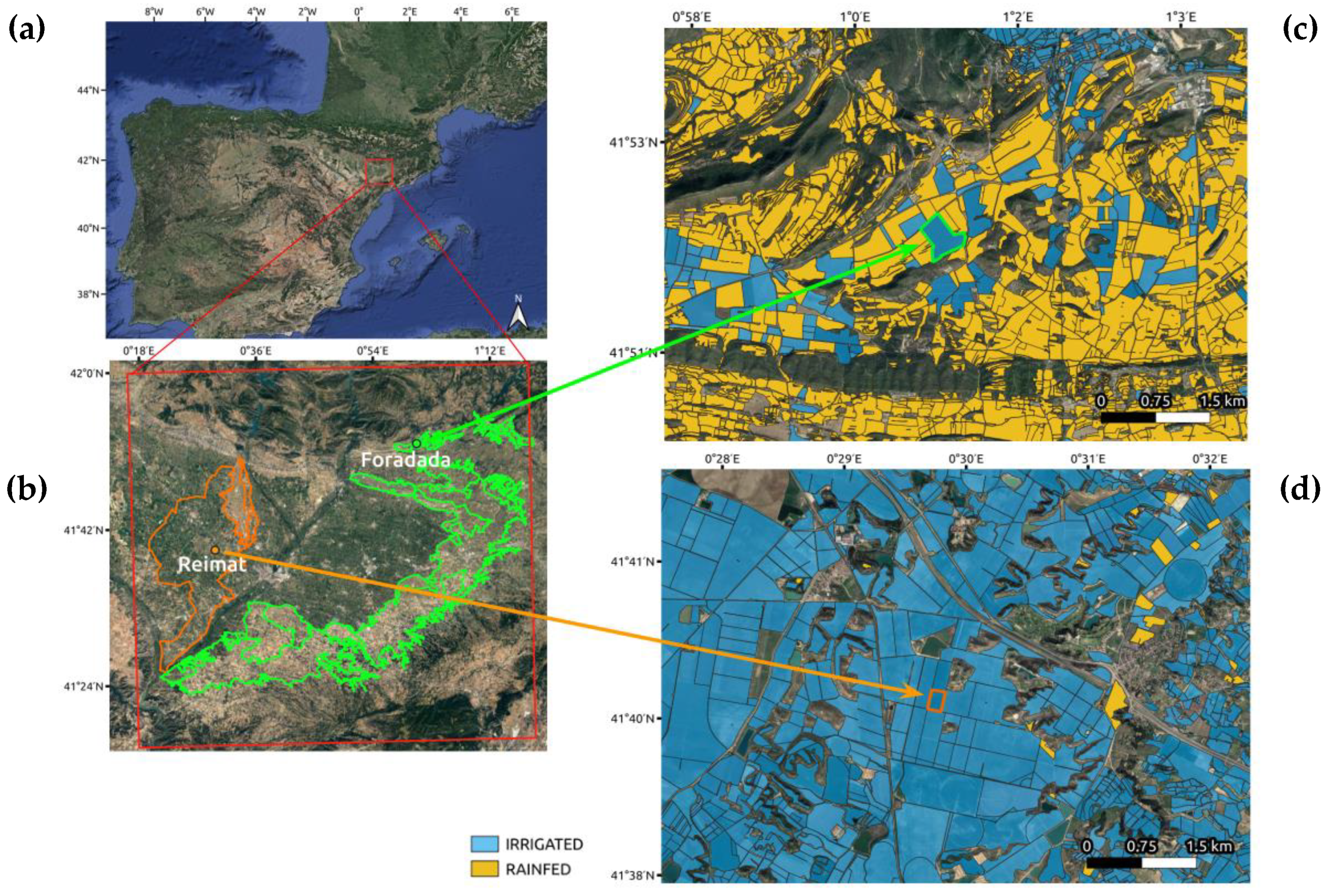
2.1. Study Area

The study area (41.28–42.02 N, 0.27–1.3 E) is located in the northeast of the Iberian Peninsula, in the province of Lleida. The considered area of interest is shown in Figure 1. In particular, in situ SSM sensors were installed in fields belonging to two different irrigation districts: three sensors were installed in a field near the village of Foradada (41.8656 N, 1.012 E) in the newly developed irrigation district of Segarra-Garrigues, while six sensors were installed in a field close to the village of Raimat (41.662 N, 0.495 E) in the Aragon and Catalonia irrigation district. Both fields were irrigated throughout the growing seasons analyzed. Foradada received a total amount of 550.2 mm of irrigated water for the period from March to October 2017 (with 90% of the total water amount used only during the summer period, from June to October). Raimat received a total amount of 491.7 mm from May to September 2018.

For the case of the Foradada field, the soil texture is 65.6% clay, 17.6% silt and 16.8% sand, and the total area of the field is 25 ha. The field was cultivated with cereals in winter and maize in the summer period. The field soil condition was very homogeneous and irrigation was applied through sprinklers in order to maintain a uniform soil water content. The field is one of the few irrigated fields in the area, with the surrounding fields being rainfed and presenting very dry soil conditions in the warmest months. As outlined in Fontanet et al., 2018 [35], these conditions are ideal to study the effectiveness of the disaggregation algorithms, since a higher SSM due to irrigation would not be recognizable at coarse spatial resolutions given the small extent of the irrigated field. In situ SSM data at 5 cm depth were available during the year 2017 at three different locations within the field. These sensors are capacitive EC-5 sensors connected to a data logger that registers soil moisture every 5 min.

In contrast to Foradada, the field in Raimat was instead surrounded by other irrigated fields, mostly vineyards, and, during 2017, it was cultivated with maize. The vegetative growth started in May until October 2017. Six different EC-5 SSM sensors were installed in the field at 5 cm depth and registered SSM at a 30 min frequency using a data logger. Fontanet et al., 2020 [36], described in detail the characteristics of the fields in terms of soil properties, irrigation practices, sowing techniques and crop types planted. The total area of the field was 5.8 ha. Irrigation was applied continuously over the entire field. It is important to notice how the differences in soil, terrain slope and agricultural management in different areas of the field lead to a heterogeneous distribution of SSM, which allows for a comprehensive analysis of sub-field SSM variations.

In order to perform a field-scale analysis, the in situ SSM time-series of the different sensors in the same field were firstly normalized, using the maximum and minimum values of each time series, and subsequently averaged together. Similarly, remotely sensed SSM were firstly extracted for each day averaging the pixels inside the field and subsequently normalized.

2.2. DisPATCh Algorithm

The details of the DisPATCh algorithm are provided in Merlin et al., 2012 [34], while in the following paragraph the general structure of DisPATCh and some additional modifications to the original algorithm are presented.

The DisPATCh disaggregation technique is based on deriving soil evaporative efficiency (SEE) from high resolution thermal and optical vegetation data, and using it for the disaggregation of low resolution SSM data. This version of DisPATCh uses a linearized relationship between SEE and SSM, according to the following formula:

$$\mathrm{M}={\mathrm{SM}}_{\mathrm{LR}}+\left(\frac{{\mathrm{SM}}_{\mathrm{LR}}}{\mathrm{mean}\left({\mathrm{SEE}}_{\mathrm{HR}}\right)}\right)·\left({\mathrm{SEE}}_{\mathrm{HR}}-\mathrm{mean}\left({\mathrm{SEE}}_{\mathrm{LR}}\right)\right)$$

(1)

where LR stands for low resolution and HR for high resolution. The SEE was calculated from the optical and thermal inputs as follow:

$${\mathrm{SEE}}_{\mathrm{HR}}=\frac{{\mathrm{T}}_{\mathrm{s},\max }-{\mathrm{T}}_{\mathrm{s},\mathrm{HR}}}{{\mathrm{T}}_{\mathrm{s},\max }-{\mathrm{T}}_{\mathrm{s},\min }}$$

(2)

where T_s,HR is the high resolution soil temperature, T_s,max and T_s,min are the extremes of the soil temperature, which correspond to the value of T_s,HR when SEE_HR equals to 1 and 0, respectively. These variables are estimated with a trapezoidal approach built in the feature space between the fractional vegetation cover (fv) and LST [34].

As proposed in Ojha et al., 2021 [37], a modification of DisPATCh for areas under high vegetation cover was added to the classic DisPATCh algorithm. This correction is applied when a large vegetation cover does not allow a correct estimation of the soil temperature from the thermal and optical data. In that case, the SEE variable is replaced by the temperature vegetation dryness index (TDVI), directly calculated from the LST values, as follows:

$${\mathrm{TDVI}}_{\mathrm{HR}}=\frac{{\mathrm{LST}}_{\max }-{\mathrm{LST}}_{\mathrm{HR}}}{{\mathrm{LST}}_{\max }-{\mathrm{LST}}_{\min }}$$

(3)

where the max and min LST are extracted from the wet and dry edges of the trapezoid built in the LST-fv feature space.

Three datasets were created using the DisPATCh disaggregation method with different satellite data at different spatial resolutions, as shown in

Table 1. Presentation of the different products produced using the DisPATCh algorithm.

Product Name	Inputs
	Low Resolution SSM	High Resolution LST	High Resolution NDVI
SMAP + MODIS (1 km)	SMAP L2 SSM	MODIS’ Terra and Aqua LST	MODIS NDVI
SMAP + S3 (1 km)	SMAP L2 SSM	Sentinel-3 SLSTR L2 LST	Sentinel-2 NDVI
SMAP + S3en (20 m)	SMAP L2 SSM	Sentinel-3 enhanced LST	Sentinel-2 NDVI

. The first two datasets, SMAP + MODIS and SMAP + S3, have a 1 km resolution while SMAP + S3en has a 20 m resolution. The SMAP + MODIS dataset is a disaggregation of SMAP SSM data at 1 km, using LST and optical/visible data from the instruments onboard MODIS’ Aqua and Terra platforms. The SMAP + S3 product was created by disaggregating SMAP SSM with the 1 km resolution LST data from the Sentinel-3 SLSTR instrument and optical/visible data from the Sentinel-2 MSI instrument, resampled at 1 km resolution. MODIS and Sentinel-3 satellites have been extensively used in the DisPATCh algorithm to disaggregate passive microwave SSM products at 1 km resolution [28,29,34,35,37,38,39]. They were also validated at different times, thus serving as a robust reference to compare the improvements of disaggregation at higher spatial resolutions. Finally, the SMAP + S3en dataset was created by disaggregating SMAP SSM data with the 20 m resolution sharpened LST product from Sentinel-3 and Sentinel-2 optical data.

2.3. Remote Sensing Data

2.3.1. SMAP SSM

The enhanced 9 km resolution L2 passive SSM product (L2_SM_P_E) from the SMAP mission [9] was selected as the baseline SSM to be downscaled. The validation of this product showed similar performances to the original SMAP L2SM product [40], but it also showed a more detailed distribution of SSM and a clearer identification of spatial features than with the standard product [41]. The enhancement was applied on the L1 brightness temperatures through the use of the Backus–Gilbert (BG) optimal interpolation technique [42,43], which exploits the radiometer intrinsic spatial oversampling [44]. This technique did not alter the initial radiometer contributing domain, which is around 33 km, but it oversampled the L1 brightness temperatures on a finer grid (9 km instead of the standard 36 km). This enhanced L1 temperature product was then used as the input in the standard SMAP pipeline, to produce the enhanced L2 SSM product.

2.3.2. Land Surface Temperature

A data fusion of two different remotely sensed products is proposed, in order to produce an LST product with high spatio-temporal resolution and overcome the limitations of directly observed LST products. The approach chosen in this paper was to use, daily, 1 km resolution Sentinel-3 SLSTR data and to apply a data sharpening technique, as proposed in Gao et al., 2012 [33], and developed in Guzinski et al., 2019 [32]. This algorithm, called data mining sharpening (DMS), was used to leverage the correlation between the low (1 km) resolution thermal data from Sentinel-3 and the high (20 m) resolution optical/near-infrared signals coming from the MSI instrument onboard the Sentinel-2 platform. The algorithm trained an ensemble of decision trees on the Sentinel-2 products, a digital elevation model (DEM) map and a map of solar incidence angles. After being trained with LST data at 1 km resolution, the model was then applied to the high resolution real data to produce 20 m resolution LST maps.

As underlined in Guzinski and Nieto, 2019 [32], the downscaled LST data set presents a limitation in terms of accuracy, given the highly non-linear relation between TIR and optical datasets, and the limited SM information contained in the reflectance data set. The observed high resolution TIR data represent a more accurate option than the downscaled data from the DMS approach. Bellvert et al., 2020 [45], compared the LST sharpened product from Sentinel-3 and Sentinel-2 data with high resolution LST data from an airborne campaign, showing a good correlation among the two datasets but a systematic underestimation (RMSE~3.5 K) of the sharpened product. This limitation in terms of absolute accuracy did not present a problem for the disaggregation algorithm presented in this paper, as DISPATCH uses relative variations of LST compared to the spatial mean. Moreover, LST is used in DisPATCh as a high resolution proxy in order to disaggregate low resolution SSM data and, as shown in Equations (2) and (3), the disaggregation leverages on the relative spatial distribution of LST inside the low resolution pixel area. For this reason, the high RMSE of the sharpened product did not directly affect the final accuracy of the disaggregated SM, while the good correlation among the datasets indicates that the sharpened LST was a suitable dataset for this application.

2.3.3. Sentinel-2 Optical Data

The normalized difference vegetation index (NDVI) at 20 m resolution was extracted from Band 4 (Red) and Band 8A (Near Infrared) of the MSI instrument onboard the Sentinel-2A and Sentinel-2B mission, with a 20 m resolution and approximately a 5-day repeating period. The bands were previously masked using the Level 2 cloud mask provided with the product.

2.3.4. Digital Elevation Model

The digital elevation model (DEM) was employed in the DisPATCh algorithm to account for the topographic effect in SSM disaggregation [39]. The shuttle radar topography mission (SRTM) provided a global DEM product with a 30 m resolution (https://doi.org/10.5066/F7PR7TFT, accessed on 15 September 2021), which is a comparable spatial scale to the final disaggregated SSM product.

3. Results

The following section is divided into three parts: first, a brief qualitative analysis over the entire area is presented for the new SMAP + S3en disaggregated product; second, a field scale qualitative analysis was performed for the two selected fields of Foradada and Raimat with available in situ data; and, lastly, a sub-field scale analysis was carried out for the same fields, investigating SSM changes inside each field. Regarding the quantitative analysis, SSM in situ data measured at 5 cm depth corresponding to the fields in Foradada and Raimat were used as a validation of the SMAP + S3en product at 20 m resolution. Two additional products at 1 km resolution, SMAP + S3 and SMAP + MODIS, were used as a benchmark to analyze the improvement.

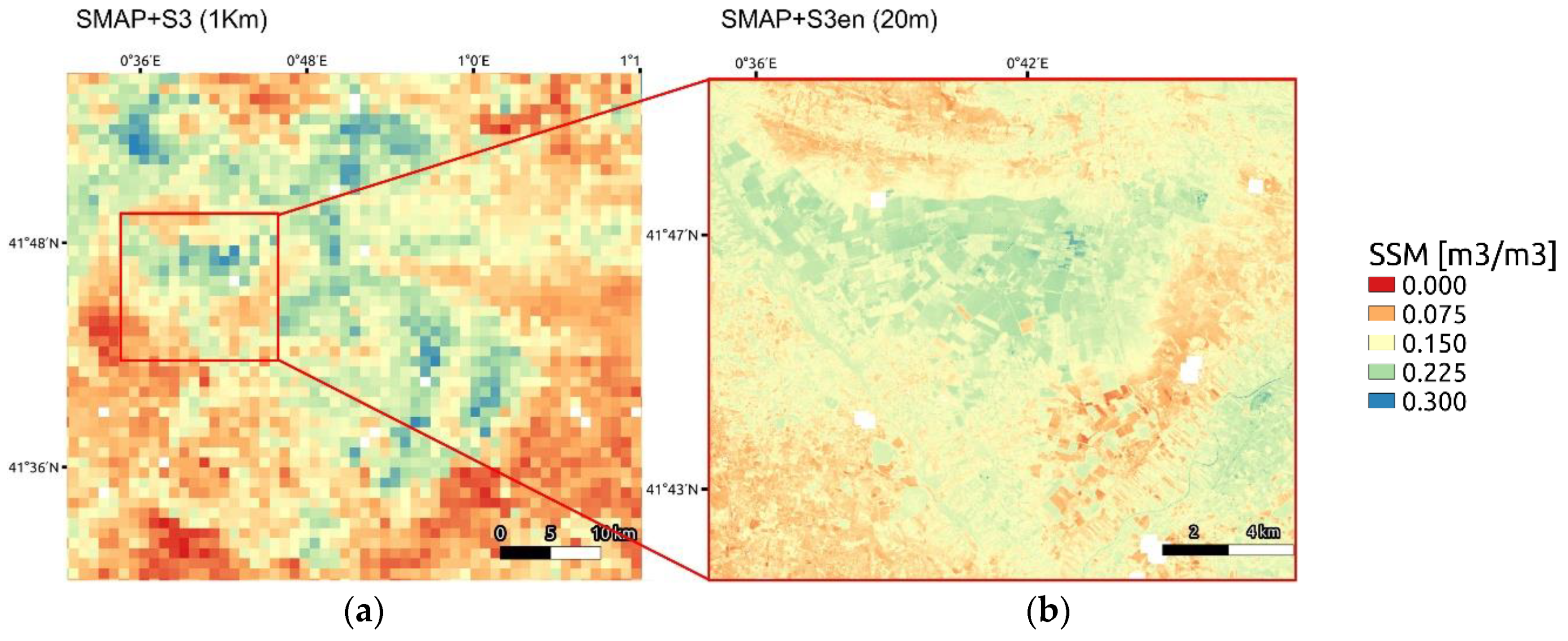
3.1. Qualitative Analysis

The disaggregated SSM product, SMAP + S3en, obtained by disaggregating SMAP data with Sentinel 3 LST data enhanced at 20 m resolution, is shown in Figure 2, where it is compared to the SSM product created by disaggregating SMAP with the original S3 data (SMAP + S3) on 19 August 2017. Improvements in the number of spatial details are noticeable from this comparison of the two products. Since the SMAP + S3en product was also derived using Sentinel-2 optical bands, it shows a different amount and position of no data pixels when compared to the SMAP + S3 product, where SSM could not be retrieved due to cloud cover in the Sentinel-2 data.

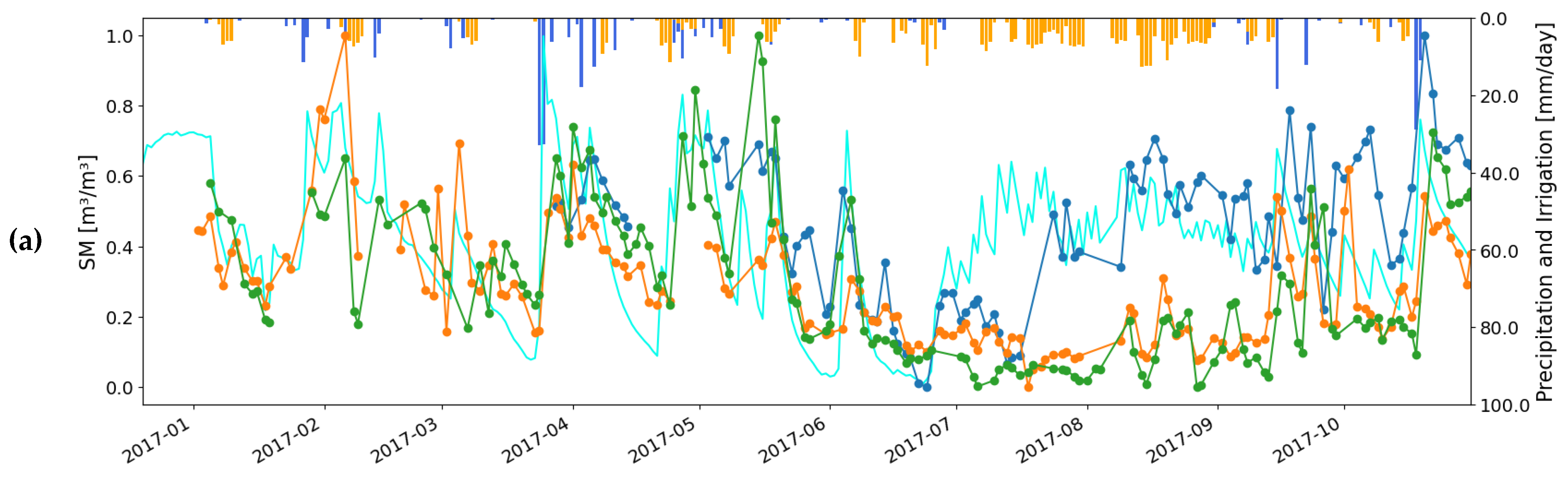
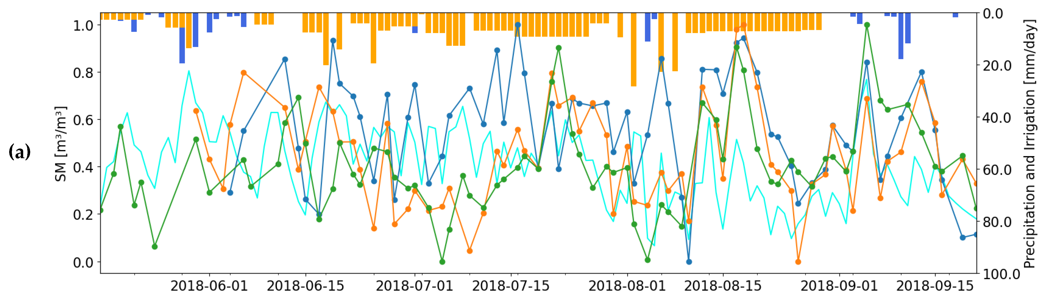
3.2. In Situ Validation at Field Scale

Figure 3 shows the time series (with in situ and remotely sensed SSM products) and scatter plot for the Foradada site during 2017. It is noticeable that, in the winter periods, all three disaggregated datasets correctly retrieved the precipitation events (blue bars in Figure 3a), showing the peaks of SSM where large precipitation events were present. At the same time, only SMAP + S3en showed an increase in SSM corresponding to irrigation events in summer (orange bars in Figure 3a). The improvements in spatial resolution of the 20 m SMAP + S3en product showed the ability to detect irrigation events, which, in this case, happened at a very limited spatial scale. All the products were able, instead, to successfully detect precipitations, since they are spatially larger events that can be recognized at coarser resolutions.

Figure 4 shows the corresponding plots for the site of Raimat during 2018, for the period from May to October 2018. Similarly to the case of Foradada, both the time series and the scatter plot showed how SMAP + S3en has a closer agreement to in situ data, even if the difference between the three disaggregated products was less marked. This can be explained by the fact that irrigation events occurred at a much larger spatial scale in the Raimat area, since all the surrounding fields were also irrigated and showed a similar SSM response: this allowed the detection of part of the irrigation events also by SSM products disaggregated at 1 km.

Table 2. Comparison of three different DisPATCh disaggregated SSM against in situ measurements.

Site	Datasets	R	Slope	Bias	GDOWN *
Foradada	SMAP + S3en	0.47	0.51	0.08	0.16
	SMAP + S3	0.39	0.27	−0.14	−0.04
	SMAP + MODIS	0.28	0.35	−0.13	0.02
	SMAP	0.39	0.33	−0.15	-
Raimat	SMAP + S3en	0.31	0.42	0.19	0.17
	SMAP + S3	0.23	0.31	0.06	0.08
	SMAP + MODIS	0.21	0.26	0.03	0.05
	SMAP	0.20	0.15	0.03	-

* GDOWN [26] shows the level of improvements of the disaggregated products with respect to the original SMAP product when compared to in situ data.

shows a summary of the results. For this particular study, the GDOWN metric [39] was proposed as a comparison tool between the 20 m and the two 1 km products disaggregated from DisPATCh. The formulation of GDOWN used here only compares the slope of the original and disaggregated product when compared with the in situ data, as follows:

$${\mathrm{G}}_{\mathrm{DOWN}}=\frac{\left|1-{\mathrm{S}}_{\mathrm{LR}}\right|-\left|1-{\mathrm{S}}_{\mathrm{HR}}\right|}{\left|1-{\mathrm{S}}_{\mathrm{LR}}\right|+\left|1-{\mathrm{S}}_{\mathrm{HR}}\right|}$$

(4)

The positive value of this metric showed how an overall improvement is detected with the product at 20 m. This improvement is also reflected by the other metrics presented: the Pearson’s correlation coefficient (R), the slope and the bias, retrieved when comparing the DisPATCh products with the in situ values.

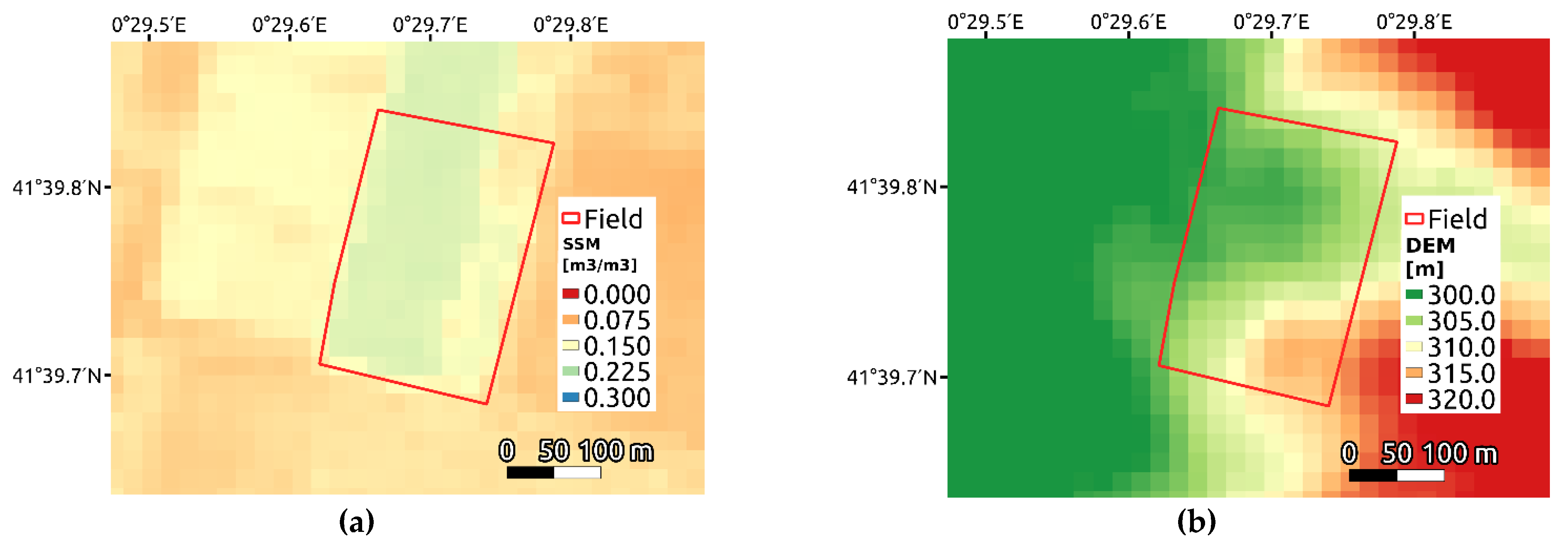
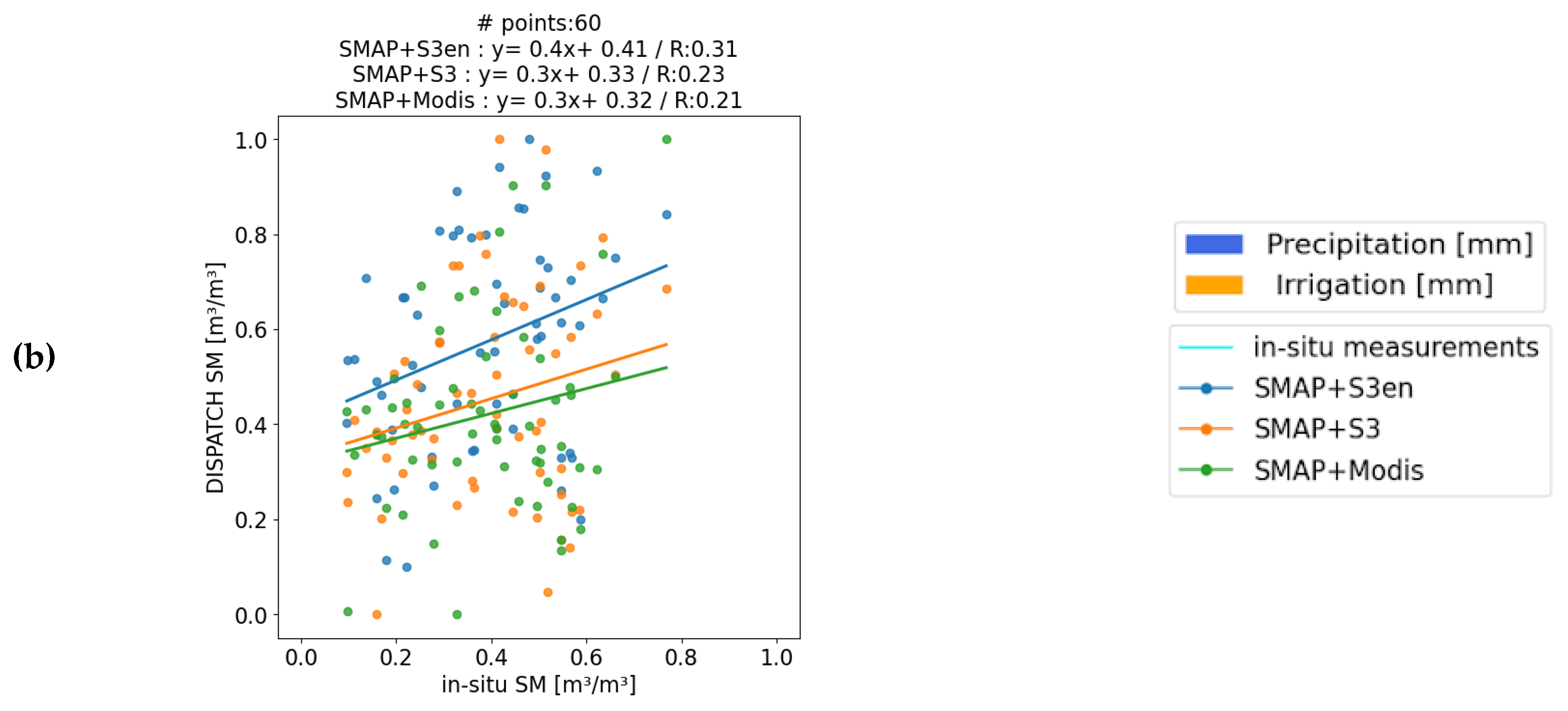
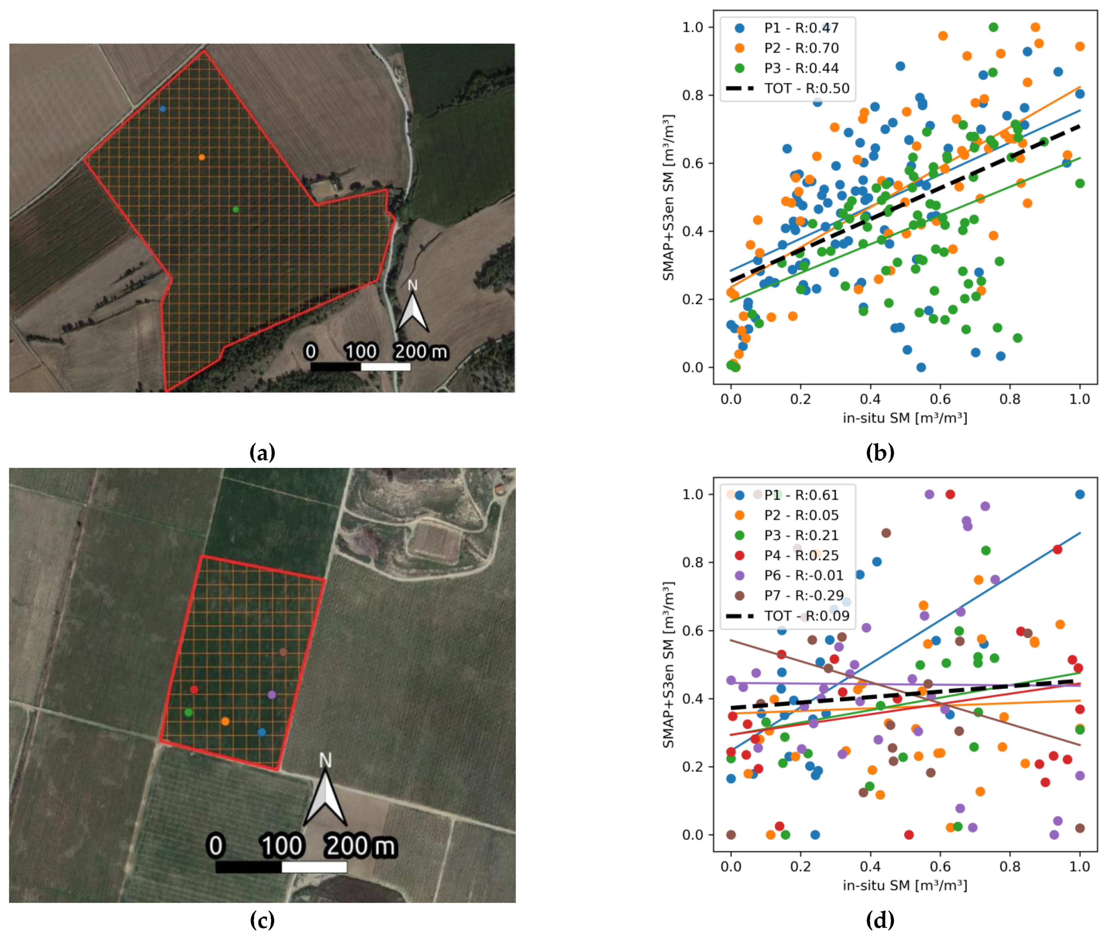
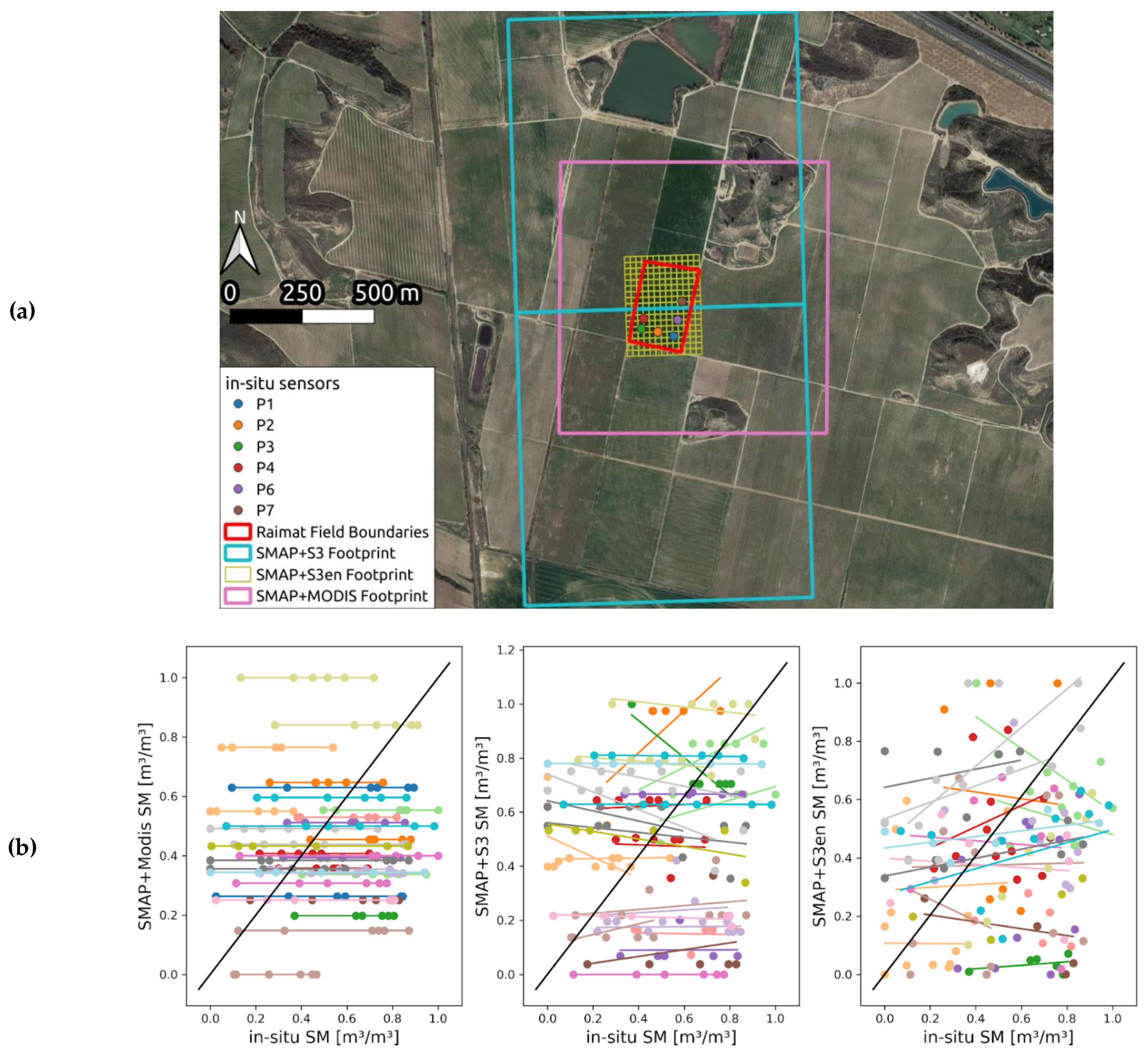
3.3. Sub-Field Scale Analysis

The very high resolution of the SMAP + S3en product presents the capability of showing local differences in SSM at sub-field scale. For the case of the Raimat field, it is noticeable how the estimated SSM was able to capture two different SSM conditions within the same field. As shown in Figure 5a, the east side of the field showed a pronounced lower SSM than the west part. These spatial differences were already observed while conducting the experimental field campaign [36] and can be explained by the topographic differences present in the area. The Raimat field presents a pronounced slope that leads water to runoff towards the west side, as seen from Figure 5b, which shows the 30 m SRTM DEM data. Figure 5a shows the average SSM derived from SMAP + S3en, during the irrigation period.

As a first sub-field scale analysis, the SSM time-series of the individual in situ sensors that were placed in the Foradada and Raimat fields have been compared against the SMAP + S3en SSM at pixel level, so that only the pixel overlapping with the sensor location are considered.

The field in Foradada showed a good correlation for all the three sensor locations (Figure 6b). The values of Pearson’s correlation coefficient at pixel level were similar to the comparison at field scale: one sensor in particular (P2) showed higher correlation values at pixel level (R = 0.70) than at field scale (R = 0.41). The total correlation computed using the pixels over all the three sensors was also slightly higher (R = 0.5) than the correlation at field level. In contrast, the correlation between the in situ and SMAP + S3en SSM for the Raimat field seemed to vary depending on the different six sensors, as shown in Figure 6d. Results were poorer compared to the average field values (R = 0.42), except for P1 (R = 0.61). These results can be partly explained by the short duration of the time series: SSM was only measured during the irrigation period, which lowered the range of measured SSM values and limited the number of usable points for this comparison. As it is noticeable from the timeseries in Figure 4a, the field in Raimat is almost continuously irrigated and no intense irrigation events are present during the three summer months considered. For this reason, the SSM signal does not contain the full range of values that goes from very wet to dry conditions, which directly affects the quality of the temporal comparison with the in situ data. In contrast, for the case of Foradada, a long time series with varying SSM conditions throughout the year is considered, as seen from Figure 3a, leading to a better correlation at sub-field scale. For this reason, an additional study is then performed, focusing on the spatial correlation of the in situ sensors with the 20 m DisPATCh product for the field in Raimat.

Since six different in situ sensors were installed in the field in Raimat, a spatial analysis was performed to verify and understand if the SSM spatial dynamic is depicted correctly with this new product. Figure 6a shows the footprints of the pixels for the three different products, and Figure 6b depicts the plots of the three disaggregated products against in situ data at each point. These results are summarized in

Table 3. Mean and standard deviation (values in parenthesis) of the daily correlation and slope coefficients between the 3 disaggregated products, and the in situ data for the field of Raimat.

Product	R (-)	Slope (-)
SMAP + MODIS	0.00 (0.00)	0.00 (0.00)
SMAP + S3	−0.14 (0.49)	−0.01 (0.25)
SMAP + S3en	0.15 (0.42)	0.03 (0.27)

, while the footprint of the pixels for these three products and their daily spatial correlations with the six in situ sensors are presented in Figure 7a,b. The average daily correlation between SMAP + MODIS and the in situ data was 0, its average daily slope was 0. This value was expected, since SMAP + MODIS does not present any spatial variability at a sub-field scale, given that only one pixel covers the entire field. Similarly, the average daily correlation and average daily slope for the SMAP + S3 product against in situ data was −0.15 and −0.01. The reason for the absence of correlation and the negative slope is still due to the different spatial extension between the SMAP + S3 pixels (1 km × 1 km) and the size of the field analyzed. Results were worse than SMAP + MODIS, since, in this case, two different pixels are covering the field, each of them only covering a part of the field together with a large remaining area occupied by the other surrounding fields, which affects the overall SSM measured. In the case of SMAP + S3en, the average daily correlation was 0.15, and its average daily slope was 0.03. SMAP + S3en provided slight improvements in the daily average slope and daily average correlation coefficient, demonstrating how a higher resolution improves the fidelity with in situ measurements.

Even though it was possible to notice certain improvements in the detection of sub-field scale dynamics for the 20 m resolution SMAP + S3en product, the correlation with in situ data was limited and it was not entirely consistent throughout the days. The capability of depicting the spatial variation of SSM at a sub-field scale for the SMAP + S3en product was degraded due to the use of a sharpened high resolution LST product, which introduces inaccuracies in the SSM disaggregation process. As pointed out by Guzinski and Nieto, 2019 [32], one of the limitations of the sharpening methodology is a strong reduction in the range of the LST values that occurs when the area considered for sharpening does not show a high contrast in terms of reflectance levels, causing a loss in spatial details. Additionally, it is not possible to overcome this limitation by extending in space or time the area subjected to the sharpening process, given that the statistical relationship between high resolution optical data with original thermal data is only present for localized cases, and degrades when increasing the spatio-temporal size of the scene considered.

4. Discussion and Conclusions

The DisPATCh algorithm has been generally used to downscale SSM from passive microwave remote sensing sensors (around 40 km spatial resolution) to a resolution of 1 km. In a few cases, it was also applied in order to reach higher resolutions, such as the 100 m product obtained by leveraging the LST data from the Landsat platforms. SSM, at the field and sub-field scale, is currently very difficult to obtain using disaggregation techniques, due to the lack of direct retrieval of very high spatio-temporal resolution LST data. The SMAP+S3en product overcomes this difficulty by using a downscaled LST product, produced by applying a sharpening algorithm to the Sentinel-3 LST original data, exploiting the high spatial resolution from Sentinel-2 optical bands.

The current manuscript presented and validated this new DisPATCh SSM product, called SMAP + S3en. This product has a 20 m resolution and a temporal frequency of 2–3 days (based on the SMAP overpass frequency) under cloud-free conditions. The validation showed a relatively good agreement with in situ data, collected for two different fields and two different years. For the Foradada field, an improvement in correlation with in situ data was achieved for the SMAP + S3en 20 m SSM product (R = 0.47) when compared with the SMAP + S3 1 km resolution SSM product (R = 0.39) and the SMAP + MODIS 1 km resolution SSM (R = 0.28) for the year 2017. Similarly, the SMAP + S3en product also showed improvements in correlation for the Raimat field during the year 2018 (R = 0.31 against R = 0.23 for SMAP + S3 and R = 0.21 for the SMAP + MODIS product).

As an additional metric for this analysis, the GDOWN [39] was calculated. This metric is particularly useful to summarize in one value the performance of the disaggregation technique: it is positive when the disaggregated SSM data are closer to in situ data than the original SSM data, while it is negative when the disaggregated data show a degraded agreement with in situ data compared to the original SSM data. The GDOWN for Foradada of the SMAP + S3en product was equal to +0.16, suggesting an improvement in the retrieval of SM, while in the case of the SMAP + MODIS the GDOWN corresponded to 0.02, suggesting only a slight improvement. The SMAP + S3 product had a slightly negative value of GDOWN, corresponding to −0.04, suggesting no improvements in the disaggregation process. The lack of improvements for the disaggregated products at 1 km resolution was already noticed by Fontanet et al., 2018 [35], which showed that the 1 km resolution is not sufficient to capture the SSM dynamics in that field, given its small size and the different behavior of the surrounding rainfed fields, which are contained in the same 1 km pixel and mask the signal from the Foradada irrigated field. This study demonstrates that the SMAP + S3en 20 m resolution product solves this issue and improves the accuracy of the retrieved SM. For the case of Raimat, GDOWN corresponded to +0.17 for SMAP + S3en, +0.08 for SMAP + S3 and +0.05 for SMAP + MODIS, proving again that the SMAP + S3en product systematically improves the agreement with in situ data.

Additionally, since the spatial resolution of SMAP + S3en is lower than the field size, sub-field scale SSM variations can be detected. For this reason, an analysis of the correlation of each in situ sensor with the overlying 20 m × 20 m pixel was performed for the three sensors installed in Foradada and the six sensors in Raimat. Results for the Foradada field showed a correlation with the in situ data at the pixel level (R = 0.44, R = 0.70 and R = 0.47), which was generally equal or better than the correlation at field level (R = 0.47). For the Raimat field, however, the results were poorer compared to the correlation at field level (R = 0.42), with the partial exception of one sensor, P1 (R = 0.61). These results can be partly explained by the short duration of the time series compared to the data in the Foradada field, and the fact that some sensors present large gaps in the SSM time-series of data collected. The lack of a long time-series of in situ data prevented a comparison of different soil conditions, as the field was continuously irrigated during the three months analyzed and no intense rain or dry periods changed the field’s water content. This temporal stability of the SM signal for the short period analyzed is also one of the causes of a lower correlation with the in situ data. Even though not all the in situ sensors of the Raimat field showed a good agreement with the remotely-sensed data, SSM spatial distribution at sub-field scale is qualitatively coherent with the topographic distribution of the field (Figure 5b).

In addition to this temporal correlation at the pixel level, for the field in Raimat, a spatial analysis was performed to better investigate the sub-field scale SSM variations. The products SMAP + MODIS, SMAP + S3 and SMAP + S3en were compared against each sensor for each available day. As expected, the estimated SSM with SMAP + MODIS did not show any significant daily average spatial correlation (R = 0) since the pixel size was higher than the entire field. For the same reason, SMAP + S3 did not show a significant regression (R = −0.14). Only SMAP + S3en showed a positive daily average spatial correlation with in situ measurements (R = 0.15), which suggest a moderate capability of this product to retrieve the general trend in sub-field scale SSM dynamics for the majority of the available days.

As a result of this entire validation process, thanks to its high spatio-temporal resolution, this product can be applied in the agricultural and water management field, improving the recent research towards remotely sensed high resolution SSM estimation. In addition, since the fine spatial resolution scale can allow the monitoring of SSM conditions at a sub-field scale, new agricultural applications, such as optimal irrigation scheduling and the detection of different management zones, can be investigated.

References

1. Daly, E.; Porporato, A. A Review of Soil Moisture Dynamics: From Rainfall Infiltration to Ecosystem Response. Environ. Eng. Sci. 2005, 22, 9–24. [Google Scholar] [CrossRef]
2. Tebbs, E.; Gerard, F.; Petrie, A.; Witte, E.D. Emerging and Potential Future Applications of Satellite-Based Soil Moisture Products. In Satellite Soil Moisture Retrieval; Elsevier: Amsterdam, The Netherlands, 2016; pp. 379–400. [Google Scholar]
3. De Jeu, R.A.M.; Wagner, W.; Holmes, T.R.H.; Dolman, A.J.; van de Giesen, N.C.; Friesen, J. Global soil moisture patterns observed by space borne microwave radiometers and scatterometers. Surv. Geophys. 2008, 29, 399–420. [Google Scholar] [CrossRef] [Green Version]
4. Mohanty, B.P.; Cosh, M.H.; Lakshmi, V.; Montzka, C. Soil moisture remote sensing: State-of-the-science. Vadose Zone J. 2017, 16, 1–9. [Google Scholar] [CrossRef] [Green Version]
5. Schmugge, T.J.; Kustas, W.P.; Ritchie, J.; Jackson, T.J.; Rango, A. Remote sensing in hydrology. Adv. Water Resour. 2002, 25, 1367–1385. [Google Scholar] [CrossRef]
6. Wagner, W.; Sabel, D.; Doubkova, M.; Bartsch, A.; Pathe, C. The Potential of Sentinel-1 for Monitoring Soil Moisture with a High Spatial Resolution At Global Scale. Earth Obs. Water Cycle Sci. 2009, 2009, 18–20. [Google Scholar]
7. Wagner, W.; Blöschl, G.; Pampaloni, P.; Calvet, J.-C.; Bizzarri, B.; Wigneron, J.-P.; Kerr, Y. Operational readiness of microwave remote sensing of soil moisture for hydrologic applications. Hydrol. Res. 2007, 38, 1–20. [Google Scholar] [CrossRef]
8. Kerr, Y.H.; Waldteufel, P.; Wigneron, J.-P.; Delwart, S.; Cabot, F.; Boutin, J.; Escorihuela, M.-J.; Font, J.; Reul, N.; Gruhier, C.; et al. The SMOS Mission: New Tool for Monitoring Key Elements of the Global Water Cycle. Proc. IEEE 2010, 98, 666–687. [Google Scholar] [CrossRef] [Green Version]
9. Entekhabi, D.; Njoku, E.G.; O’neill, P.E.; Kellogg, K.H.; Crow, W.T.; Edelstein, W.N.; Entin, J.K.; Goodman, S.D.; Jackson, T.J.; Johnson, J.; et al. The Soil Moisture Active Passive (SMAP) Mission. Proc. IEEE 2010, 98, 704–716. [Google Scholar] [CrossRef]
10. Peng, J.; Loew, A.; Merlin, O.; Verhoest, N.E.C. A review of spatial downscaling of satellite remotely sensed soil moisture. Rev. Geophys. 2017, 55, 341–366. [Google Scholar] [CrossRef]
11. Sabaghy, S.; Walker, J.P.; Renzullo, L.J.; Jackson, T.J. Spatially enhanced passive microwave derived soil moisture: Capabilities and opportunities. Remote Sens. Environ. 2018, 209, 551–580. [Google Scholar] [CrossRef]
12. Narayan, U.; Lakshmi, V.; Jackson, T.H. High-resolution change estimation of soil moisture using L-band radiometer and radar observations made during the SMEX02 experiments. IEEE Trans. Geosci. Remote Sens. 2006, 44, 1545–1554. [Google Scholar] [CrossRef]
13. Das, N.N.; Dara, E.; Njoku, E.G. An Algorithm for Merging Smap Radiometer and Radar Data for High-Resolution Soil-Moisture Retrieval. IEEE Trans. Geosci. Remote Sens. 2011, 49, 1504–1512. [Google Scholar] [CrossRef]
14. Ines, A.V.M.; Mohanty, B.P.; Shin, Y. An unmixing algorithm for remotely sensed soil moisture. Water Resour. Res. 2013, 49, 408–425. [Google Scholar] [CrossRef]
15. Reichle, R.H.; Koster, R.D. Global assimilation of satellite surface soil moisture retrievals into the NASA Catchment land surface model. Geophys. Res. Lett. 2005, 32. [Google Scholar] [CrossRef]
16. Kaheil, Y.H.; Gill, M.K.; McKee, M.; Bastidas, L.A.; Rosero, E. Downscaling and assimilation of surface soil moisture using ground truth measurements. IEEE Trans. Geosci. Remote Sens. 2008, 46, 1375–1384. [Google Scholar] [CrossRef]
17. Kim, G.; Barros, A.P. Downscaling of remotely sensed soil moisture with a modified fractal interpolation method using contraction mapping and ancillary data. Remote Sens. Environ. 2002, 83, 400–413. [Google Scholar] [CrossRef]
18. Sabaghy, S.; Walker, J.P.; Renzullo, L.J.; Akbar, R.; Chan, S.; Chaubell, J.; Das, N.; Dunbar, R.S.; Entekhabi, D.; Gevaert, A.; et al. Comprehensive analysis of alternative downscaled soil moisture products. Remote Sens. Environ. 2020, 239, 111586. [Google Scholar] [CrossRef]
19. Gao, Q.; Zribi, M.; Escorihuela, M.; Baghdadi, N. Synergetic Use of Sentinel-1 and Sentinel-2 Data for Soil Moisture Mapping at 100 m Resolution. Sensors 2017, 17, 1966. [Google Scholar] [CrossRef] [PubMed] [Green Version]
20. Hajj, M.E.; Baghdadi, N.; Zribi, M.; Bazzi, H. Synergic Use of Sentinel-1 and Sentinel-2 Images for Operational Soil Moisture Mapping at High Spatial Resolution over Agricultural Areas. Remote Sens. 2017, 9, 1292. [Google Scholar] [CrossRef] [Green Version]
21. Bazzi, H.; Baghdadi, N.; Hajj, M.E.; Zribi, M.; Belhouchette, H. A Comparison of Two Soil Moisture Products S2MP and Copernicus-SSM Over Southern France. IEEE J. Sel. Top. Appl. Earth Obs. Remote Sens. 2019, 12, 3366–3375. [Google Scholar] [CrossRef]
22. Amazirh, A.; Merlin, O.; Er-Raki, S.; Gao, Q.; Rivalland, V.; Malbeteau, Y.; Khabba, S.; Escorihuela, M.J. Retrieving Surface Soil Moisture between Sentinel-1 radar and Landsat thermal data: A study case over bare soil. Remote Sens. Environ. 2018, 211, 321–337. [Google Scholar] [CrossRef]
23. Fang, B.; Lakshmi, V.; Bindlish, R.; Jackson, T.J. Downscaling of SMAP soil moisture using land surface temperature and vegetation data. Vadose Zone J. 2018, 17, 1–15. [Google Scholar] [CrossRef] [Green Version]
24. Chen, N.; He, Y.; Zhang, X. NIR-Red Spectra-Based Disaggregation of SMAP Soil Moisture to 250 m Resolution Based on OzNet in Southeastern Australia. Remote Sens. 2017, 9, 51. [Google Scholar] [CrossRef] [Green Version]
25. Tomer, S.K.; Al Bitar, A.; Sekhar, M.; Zribi, M.; Bandyopadhyay, S.; Kerr, Y. MAPSM: A spatio-temporal algorithm for merging soil moisture from active and passive microwave remote sensing. Remote Sens. 2016, 8, 990. [Google Scholar] [CrossRef] [Green Version]
26. Piles, M.; Camps, A.; Vall-Llossera, M.; Corbella, I.; Panciera, R.; Rudiger, C.; Kerr, Y.H.; Walker, J. Downscaling SMOS-derived soil moisture using MODIS visible/infrared data. IEEE Trans. Geosci. Remote Sens. 2011, 49, 3156–3166. [Google Scholar] [CrossRef]
27. Merlin, O.; Chehbouni, A.; Walker, J.P.; Panciera, R.; Kerr, Y.H. A simple method to disaggregate passive microwave-based soil moisture. IEEE Trans. Geosci. Remote Sens. 2008, 46, 786–796. [Google Scholar] [CrossRef] [Green Version]
28. Merlin, O.; Escorihuela, M.J.; Mayoral, M.A.; Hagolle, O.; Bitar, A.A.; Kerr, Y. Self-calibrated evaporation-based disaggregation of SMOS soil moisture: An evaluation study at 3 km and 100 m resolution in Catalunya, Spain. Remote Sens. Environ. 2013, 130, 25–38. [Google Scholar] [CrossRef] [Green Version]
29. Oiha, N.; Merlin, O.; Molero, B.; Sucre, C.; Olivera, L.; Rivalland, V.; Er-Raki, S. Sequential Downscaling of the SMOS Soil Moisture at 100 M Resolution Via a Variable Intermediate Spatial Resolution. In Proceedings of the IGARSS 2018—2018 IEEE International Geoscience and Remote Sensing Symposium, Valencia, Spain, 22–27 July 2018. [Google Scholar]
30. Hulley, G.; Hook, S.; Fisher, J.; Lee, C. ECOSTRESS, A NASA Earth-Ventures Instrument for studying links between the water cycle and plant health over the diurnal cycle. In Proceedings of the 2017 IEEE International Geoscience and Remote Sensing Symposium (IGARSS), Fort Worth, TX, USA, 23–28 July 2017. [Google Scholar]
31. Fisher, J.B.; Lee, B.; Purdy, A.J.; Halverson, G.H.; Dohlen, M.B.; Cawse-Nicholson, K.; Wang, A.; Anderson, R.G.; Aragon, B.; Arain, M.A.; et al. ECOSTRESS: NASA’s Next Generation Mission to Measure Evapotranspiration from the International Space Station. Water Resour. Res. 2020, 56, e2019WR026058. [Google Scholar] [CrossRef]
32. Guzinski, R.; Nieto, H. Evaluating the feasibility of using Sentinel-2 and Sentinel-3 satellites for high-resolution evapotranspiration estimations. Remote Sens. Environ. 2019, 221, 157–172. [Google Scholar] [CrossRef]
33. Gao, F.; Kustas, W.; Anderson, M. A Data Mining Approach for Sharpening Thermal Satellite Imagery over Land. Remote Sens. 2012, 4, 3287–3319. [Google Scholar] [CrossRef] [Green Version]
34. Merlin, O.; Rudiger, C.; Bitar, A.A.; Richaume, P.; Walker, J.P.; Kerr, Y.H. Disaggregation of SMOS Soil Moisture in Southeastern Australia. IEEE Trans. Geosci. Remote Sens. 2012, 50, 1556–1571. [Google Scholar] [CrossRef] [Green Version]
35. Fontanet, M.; Fernàndez-Garcia, D.; Ferrer, F. The value of satellite remote sensing soil moisture data and the DISPATCH algorithm in irrigation fields. Hydrol. Earth Syst. Sci. 2018, 22, 5889–5900. [Google Scholar] [CrossRef] [Green Version]
36. Fontanet, M.; Scudiero, E.; Skaggs, T.H.; Fernàndez-Garcia, D.; Ferrer, F.; Rodrigo, G.; Bellvert, J. Dynamic Management Zones for Irrigation Scheduling. Agric. Water Manag. 2020, 238, 106207. [Google Scholar] [CrossRef]
37. Ojha, N.; Merlin, O.; Suere, C.; Escorihuela, M.J. Extending the Spatio-Temporal Applicability of DISPATCH Soil Moisture Downscaling Algorithm: A Study Case Using SMAP, MODIS and Sentinel-3 Data. Front. Environ. Sci. 2021, 9, 40. [Google Scholar] [CrossRef]
38. Molero, B.; Merlin, O.; Malbéteau, Y.; Bitar, A.A.; Cabot, F.; Stefan, V.; Kerr, Y.; Bacon, S.; Cosh, M.; Bindlish, R.; et al. SMOS disaggregated soil moisture product at 1 km resolution: Processor overview and first validation results. Remote Sens. Environ. 2016, 180, 361–376. [Google Scholar] [CrossRef]
39. Merlin, O.; Malbéteau, Y.; Notfi, Y.; Bacon, S.; Khabba, S.; Jarlan, L. Performance Metrics for Soil Moisture Downscaling Methods: Application to DISPATCH Data in Central Morocco. Remote Sens. 2015, 7, 3783–3807. [Google Scholar] [CrossRef] [Green Version]
40. Chan, S.; Bindlish, R.; O’neill, P.; Jackson, T.; Njoku, E.; Dunbar, S.; Chaubell, J.; Piepmeier, J.; Yueh, S.; Entekhabi, D.; et al. Development and assessment of the SMAP enhanced passive soil moisture product. Remote Sens. Environ. 2018, 204, 931–941. [Google Scholar] [CrossRef] [Green Version]
41. O’Neill, P.; Chan, S.; Bindlish, R.; Chaubell, M.; Colliander, A.; Chen, F.; Dunbar, S.; Jackson, T.; Peng, J.; Cosh, M.; et al. Soil Moisture Active Passive (SMAP) Project: Calibration and Validation for the L2/3_SM_P Version 7 and L2/3_SM_P_E Version 4 Data Products; Technical Report JPL D-56297; Jet Propulsion Laboratory, California Institute of Technology: Pasadena, CA, USA, 2020. [Google Scholar]
42. Poe, G. Optimum interpolation of imaging microwave radiometer data. IEEE Trans. Geosci. Remote Sens. 1990, 28, 800–810. [Google Scholar] [CrossRef] [Green Version]
43. Stogryn, A. Estimates of brightness temperatures from scanning radiometer data. IEEE Trans. Antennas Propag. 1978, 26, 720–726. [Google Scholar] [CrossRef]
44. Chaubell, J.; Yueh, S.; Entekhabi, D.; Peng, J. Resolution enhancement of SMAP radiometer data using the Backus Gilbert optimum interpolation technique. In Proceedings of the 2016 IEEE International Geoscience and Remote Sensing Symposium (IGARSS), Beijing, China, 10–15 July 2016. [Google Scholar]
45. Bellvert, J.; Jofre-Ĉekalović, C.; Pelechá, A.; Mata, M.; Nieto, H. Feasibility of Using the Two-Source Energy Balance Model (TSEB) with Sentinel-2 and Sentinel-3 Images to Analyze the Spatio-Temporal Variability of Vine Water Status in a Vineyard. Remote Sens. 2020, 12, 2299. [Google Scholar] [CrossRef]
Figure 1. Study area considered. (a) General identification of the area located in Lleida’s region (Catalunya). (b) Segarra-Garrigues (green) and Aragó i Catalunya (orange) irrigation districts, and the location of the two studied fields. (c) Detailed map of the Foradada field. (d) Raimat field, highlighting the surrounding irrigated and rainfed fields from the SIGPAC database (http://sig.gencat.cat/visors/Cultius_DUN_SIGPAC.html, accessed on 15 September 2021).
Remotesensing 14 00167 g001
Figure 2. SSM map of the considered study area on 19 August 2017. (a) SMAP + S3 SSM map at 1 km resolution and (b) SMAP + S3en SSM map at 20 m resolution.
Remotesensing 14 00167 g002
Figure 3. Time series (a) of in situ SSM (cyan) compared with the DisPATCh products: SMAP + MODIS (green), SMAP + S3 (orange) and SMAP + S3en (blue). The time series correspond to the data extracted in 2017 for the Foradada field, normalized to be comparable among each other. Scatter plot (b) of in situ data compared with the three DisPATCh products and their respective regression lines (same colors used). The text above the figure shows the number of points considered, the regression line formula and the Pearson’s correlation coefficient (R). The number of points considered is equivalent for each product, since only the dates for which all the products are available are considered.
Remotesensing 14 00167 g003aRemotesensing 14 00167 g003b
Figure 4. Same description as for Figure 3. (a) Time series of SSM products (in situ and DisPATCh products) that correspond to the data extracted in 2018 for the Raimat field. (b) Scatter plot of in situ data compared with the three DisPATCh products (same colors as for Figure 4a).
Remotesensing 14 00167 g004aRemotesensing 14 00167 g004b
Figure 5. Sub-field scale analysis. (a) Average of SMAP + S3en SSM during the 2018 irrigation period for the Raimat field (03 May 2018–07 September 2018). (b) SRTM DEM map of the Raimat field.
Remotesensing 14 00167 g005
Figure 6. Sub-field scale correlation analysis: (a) position of the three in situ sensors in the Foradada field and pixel sizes of the SMAP + S3en SSM product. (b) Scatter plot of SMAP + S3en SM data at pixel level vs the in situ data for each single sensor for the Foradada field. (c) Position of the six in situ sensors for the Raimat field and pixel sizes of the SMAP + S3en SSM product. (d) Scatter plot and correlations for each location of the sensors for the Raimat field.
Remotesensing 14 00167 g006
Figure 7. Spatial analysis for the field in Raimat. (a) Footprints of the different pixel sizes of the product used. For the case of SMAP + MODIS (pink), a single pixel covers the entire area, showing the same value for the six different sensors, while in the case of SMAP + S3 (cyan) the sensor in position P7 is covered by a different pixel. SMAP + S3en (yellow) has a finer resolution where each pixel covers a different sensor. The six points representing the sensors’ positions have been magnified for the sake of visibility, each of them is actually contained in a 20 m by 20 m SMAP + S3en pixel. (b) Spatial correlation for each available day for the 3 different products, SMAP + MODIS, SMAP + S3 and SMAP + S3en.
Remotesensing 14 00167 g007