Article

The Dynamic Relationship between Air and Land Surface Temperature within the Madison, Wisconsin Urban Heat Island

by
Elizabeth Berg
1,* and
Christopher Kucharik
1,2
1
Nelson Institute for Environmental Studies, University of Wisconsin-Madison, Madison, WI 53706, USA
2
Department of Agronomy, University of Wisconsin-Madison, Madison, WI 53706, USA
*
Author to whom correspondence should be addressed.
Remote Sens. 2022, 14(1), 165; https://doi.org/10.3390/rs14010165
Submission received: 29 October 2021 / Revised: 8 December 2021 / Accepted: 28 December 2021 / Published: 31 December 2021
(This article belongs to the Special Issue Urban Sensing Methods and Technologies)

Abstract

:
The urban heat island (UHI) effect, the phenomenon by which cities are warmer than rural surroundings, is increasingly important in a rapidly urbanizing and warming world, but fine-scale differences in temperature within cities are difficult to observe accurately. Networks of air temperature (Tair) sensors rarely offer the spatial density needed to capture neighborhood-level disparities in warming, while satellite measures of land surface temperature (LST) do not reflect the air temperatures that people physically experience. This analysis combines both Tair measurements recorded by a spatially-dense stationary sensor network in Dane County, Wisconsin, and remotely-sensed measurements of LST over the same area—to improve the use and interpretation of LST in UHI studies. The data analyzed span three summer months (June, July, and August) and eight years (2012–2019). Overall, Tair and LST displayed greater agreement in spatial distribution than in magnitude. The relationship between day of the year and correlation was fit to a parabolic curve (R2 = 0.76, p = 0.0002) that peaked in late July. The seasonal evolution in the relationship between Tair and LST, along with particularly high variability in LST across agricultural land cover suggest that plant phenology contributes to a seasonally varying relationship between Tair and LST measurements of the UHI.

1. Introduction

In the context of a rapidly urbanizing planet [1,2] and rising global temperatures [3], the extra heat burden experienced in cities raises concern. The common pattern of increased temperatures in cities, referred to as the urban heat island (UHI) effect, has been tied to poor air quality [4], increased energy consumption [5,6], and multiple health risks, including increased mortality [7]. Extreme heat is already one of the deadliest weather-related threats [8], and the combined effect of climate change and urbanization are expected to increase dangerous exposure to extreme heat among urban populations [9]. Detailed and accurate monitoring of UHIs is needed to adequately predict and prepare for extreme heat risk [10,11].
Historically, a variety of data sources have been used to observe and analyze UHIs, each with its own advantages and drawbacks. Observational studies may rely on measurements from pairs of urban and rural air temperature (Tair) sensors (e.g., [12]) or use networks of dozens or hundreds of sensors [13]. Mobile sensors have also been used to measure Tair at high spatial resolution along urban transects [14,15,16,17]. These mobile transects typically cannot provide a historical temperature record, while weather stations that offer a long historic record may provide limited spatial coverage, and few high-density sensor networks have been maintained for longer than five years [13]. Therefore, an alternative to using Tair measurements to study the canopy-level UHI is studying the surface urban heat island (SUHI) with satellite data [18]. Satellite measurements of land surface temperature (LST) have been used in UHI research since 1972 [19], but these methods have increased exponentially since 2005 due to advances in remote sensing and big data analysis techniques [18]. Because satellite data can offer long historic records and continuous spatial coverage over large swaths of land, albeit, with limited sampling frequency, remotely-sensed LST can be used for applications such as studying how the UHI changes as a city grows, comparing UHIs across multiple cities, and correlating temperatures with land cover [20,21].
Although both the canopy-level UHI and the SUHI are used in urban climate studies, Tair and LST are not directly analogous [18,20]. People can physically experience the difference between high and low air temperatures, but it is less clear whether satellite-derived LST accurately captures short-term excessive heat conditions that threaten human health [22]. Given the ubiquity of satellite data in UHI studies, it is important to understand if and how remotely-sensed LST reflects the temperature conditions that urban residents physically experience. These questions of how Tair and LST relate to each other and whether one can be used to predict the other have been widely explored, in both urban and non-urban settings.
In homogeneous rural environments, LST is generally predictive of Tair, but this relationship is impacted by other variables, including cloud cover, wind, time of day, season, and surrounding land cover [23,24,25,26]. Typically, LST experiences greater diurnal variability than Tair, reaching higher temperatures during the day and lower temperatures overnight [22,27]. The magnitude of the difference between LST and Tair is greatest, and correlation is lowest, during the summer season and in the early afternoon, when both air temperatures and LST are highest [23,28]. Windy and cloudy conditions have consistently been found to decrease the magnitude of the difference between LST and Tair and increase the correlation between these two measures of temperature [20,23,24,27]. However, satellite data is often unavailable or less accurate under cloudy conditions [29]. Variability in the surrounding land cover is another factor that can decrease the correlation between Tair and LST [20]; as a result, some of the strongest linear relationships between Tair and LST have been observed across locations that were specifically selected for their consistent surrounding year-round vegetated cover [23,27].
Due to the heterogeneity of the urban landscape, the relationship between Tair and LST is more complex in these settings, and past analyses of this relationship have revealed mixed results [14,18,30,31]. The temperature range observed in the SUHI is typically greater than the difference between urban and rural Tair, and the magnitude of the SUHI usually peaks during the day, rather than the night-time peak observed in the canopy-level UHI [32]. Despite these typical patterns, the variables that shape the relationship between urban Tair and LST depend on each city’s unique geography [31]. In Vancouver, Canada, Tair recorded at weather stations across the city and Landsat LST observations were found to be poorly correlated [33]. Similarly, no correlation was observed between the magnitude of the Tair and LST-based UHIs in Hangzhou, China, regardless of the season or time of day [34]. Studies in both Leipzig, Germany, and Birmingham, UK produced high correlations between measurements of Tair and LST and a weaker relationship between the magnitude of the SUHI and the canopy level [14,35]. Overall, no consistent and universal relationship has been established between these two different measures of temperatures in urban environments [18,20].
Cities that have been the subject of past Tair and LST comparisons, such as Vancouver, Los Angeles, Hangzhou, and Birmingham, generally have large populations, with more than one million residents in their surrounding metropolitan areas [31,33,34,35]. Networks of urban temperature sensors are most commonly in cities with similarly large populations [13]. Urban warming is often greatest in the most populated cities, and these trends certainly merit further research [17]; however, only a minority of urban residents live in the largest cities [36]. In the U.S., for example, less than 8% of the population lives in cities with over 1,000,000 residents, while nearly twice as many people live in cities with populations between 100,000 and 500,000 [36]. Our analysis focuses on one of these less populated U.S. urban areas: the city of Madison, Wisconsin, which has a population of 258,000, and the surrounding county, which has a total population of 547,000 over roughly 3100 km2 (1200 mi2) of land [37].
This study uses data from a spatially dense network of air temperature sensors throughout the Madison area to build on past investigations of the relationship between the SUHI and canopy-level UHI. In addition to its high spatial resolution, our sensor array is distinguished by the diversity of land use covered. Although most of the network is within city limits, 40% of the sensors are located outside these boundaries, providing coverage of agricultural land dominated by annual crops, as well as nearby forest, grasslands, wetlands, and neighboring towns [13]. Similar to other mid-sized cities in the Corn Belt, land cover in Madison quickly transitions from urban development to cropland near the city limits [38]. The spatial density of the Madison sensor network allows for a uniquely detailed examination of how urban warming varies across a representative Midwest city. By comparing Tair measured by this sensor network with satellite measurements of summer LST, we investigate how accurately the SUHI represents Tair across the heterogeneous landscape of Dane County, Wisconsin. This study explores how the relationship between summer Tair and LST changes with land cover and throughout the growing season. By comparing Tair and LST along these lines, we can better understand when and how to use satellite data to study urban warming in a mid-sized city within a heterogeneous agricultural region.

2. Materials and Methods
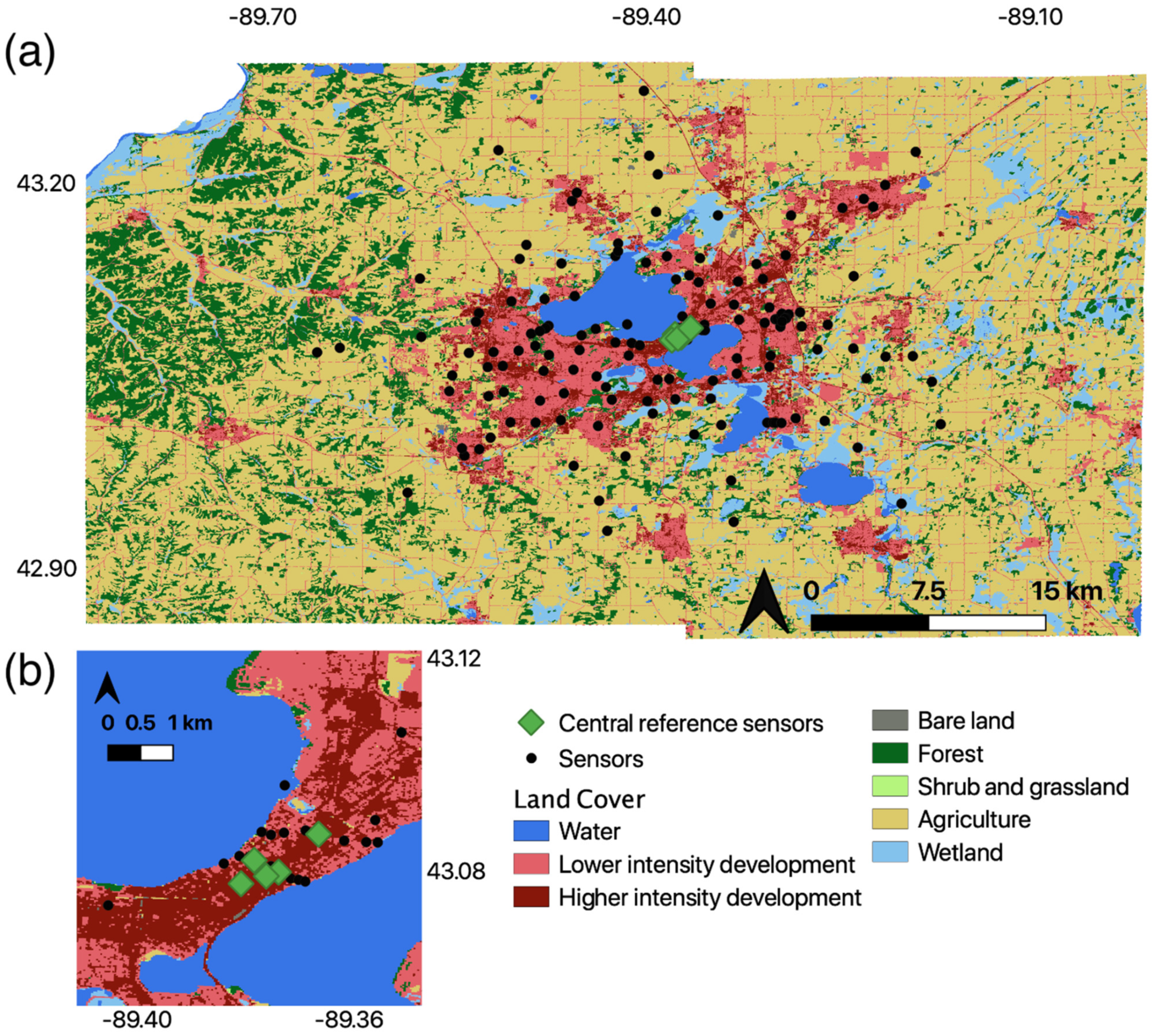
2.1. Study Area

This study focuses on Dane County (Wisconsin) and the city of Madison, located near the center of the county. Dane County has a population of roughly 547,000, and nearly half of the county’s residents (260,000 total) live within the city of Madison [37]. A chain of four lakes lies within and around the city. The county’s rural areas are primarily agricultural, but also contain forest, wetlands, and grasslands (Figure 1a). Across Dane County, 15% of the land area is developed and 46% of the area is cropland, with corn and soybeans the two most commonly grown crops [39].

2.2. Satellite Data

This analysis uses Landsat 7 and Landsat 8 scenes from the U.S. Geological Survey (USGS) Analysis Ready Data (ARD) Provisional Surface Temperature product. These two sensors have different thermal band wavelengths (10.4–12.5 µm for Landsat 7 and 10.6–11.2 µm for Landsat 8 band 10) and resolutions (60 m for Landsat 7 and 100 m for Landsat 8), but USGS produces 30-m LST from both, using higher resolution input from visible and shortwave bands to resample the coarser thermal data [40]. The USGS ARD product was chosen for this analysis due to the detailed land surface emissivity incorporated in these data [40]. Calculating LST requires measurements of the radiance received at the satellite, as well as knowledge of the sensor viewing angle, thermal band wavelength, the emissivity of the land surface, and atmospheric transmissivity, path radiance, and downwelling irradiance [40]. The sensor measurements, viewing angle, and thermal wavelength are straightforward to measure, and the atmospheric parameters can be calculated with a radiative transfer model [40]. However, estimating surface emissivity is more difficult, as it requires inputs that are independent of the sensor, and small errors in emissivity can produce much larger errors in LST [40]. Instead of using land cover classifications or vegetation indices to estimate emissivity [40,41], the USGS ARD product incorporates emissivity from the Advanced Spaceborne Thermal Emission and Reflection Radiometer (ASTER) Global Emissivity Data Set (GED) [42]. This dataset averages millions of ASTER datapoints collected between 2000 to 2008 to produce a monthly worldwide database at 100 m resolution with an error of roughly 1% [42]. Because surface emissivity is more precisely known over water than the land surface, the USGS ARD product has been found to have an average error of less than 1 °C over water and 2.2–2.3 °C over land [40].
We limited this analysis to the summer months (June through August), which is when urban warming poses the greatest threat to human health and when Madison’s urban-rural temperature difference is largest [13]. We further limited the study period to the years from 2012 through 2019 to overlap all eight years that the Madison temperature sensor network has been operational. Using the USGS EarthExplorer tool, we initially identified 101 Landsat 7 or Landsat 8 scenes recorded during this study period. Because clouds emit radiation at lower temperatures than the land surface that they obscure, scenes with heavy cloud cover are not usable for LST analysis [43]. After filtering for dates with less than 30% cloud cover and visually inspecting the results to eliminate scenes where clouds obscured Dane County, we chose 15 dates, including at least one scene from each year of the study period and a relatively even distribution across both satellites and all three summer months (Table 1). Although all 15 dates had clear skies, meteorological conditions were otherwise representative of the typical range seen during the summer in Madison, with daily low temperatures ranging from 8.9 °C to 21.7 °C, daily highs ranging from 21.7 °C to 33.9 °C, and daily wind speeds between a mean of 1.21 m/s and 4.47 m/s and a maximum of 3.58 m/s and 8.05 m/s (Table 1).
Because Dane County spans two tiles on the ARD grid (h20v07 and h20v06), 30 scenes were downloaded in total. Unlike other satellite products that use temporally variable tile boundaries, ARD tiles are defined with fixed, non-overlapping coordinates so that adjacent scenes can be mosaicked without requiring additional processing [44]. Therefore, after masking cloudy pixels and scan line artifacts, the two scenes for each date were simply stitched together using ENVI’s Seamless Mosaic tool, then clipped to Dane County boundaries. We also chose to mask the water area from all 15 Landsat scenes, because the sensor network does not extend over the local lakes, preventing comparison between LST and Tair over these areas. The resulting 30m Landsat scenes were used in the land cover analysis after these processing steps. However, the comparisons between LST and Tair required both datasets to share the same spatial resolution. The interpolated sensor data has a 400 m resolution, so we needed to reduce the resolution of each Landsat scene from 30 m to 400 m, using the “aggregate” function in R’s raster package [45]. Because 30 m is not an integer factor of 400 m, aggregating the Landsat scenes to this coarser resolution required resampling the raster. Aggregating and resampling satellite data can introduce errors and reduce the level of detail in spatial patterns, occasionally distorting or obscuring patterns entirely [46,47]; however, this processing was necessary to produce LST data files that could be compared with Tair.

2.3. Stationary Air Temperature Data

The Tair data used in this analysis comes from an observational network of 146 HOBO U23 Pro v2 temperature and relative humidity data loggers mounted on utility poles throughout the Madison area. Each sensor is installed 3.5 m above the ground, a height that was chosen to avoid damage from passing pedestrians or vehicles. The first 135 sensors were launched in March 2012, 16 more were added over the following year, and five sensors have been broken or lost since then. This sensor array has been recording Tair and relative humidity measurements every 15 min since being launched. This network, one of the largest and densest in the world, is described more fully in [13]. To provide a consistent comparison with the LST data, this analysis used Tair measurements collected on the same days as the satellite data. All 15 Landsat scenes were recorded between 11:30 a.m. and 11:45 a.m. local time, so we selected sensor measurements from 11:30 a.m. local time to understand the relationship between approximately simultaneous Tair and LST conditions. Additionally, because the differences in magnitude between Tair and LST are often greatest near noon [23] and past research [31,48] has found satellite-derived LST to be more closely correlated to Tair at night than during the day, we also used Tair measurements from 12 h prior to each satellite overpass (11:30 pm) to allow for analysis of the relationship between LST and overnight Tair.
For all 15 dates studied, 400-m spatial interpolations of daytime and nighttime Tair were produced using regression kriging, a technique that incorporates land surface covariates and has been found to produce more accurate spatial models of urban temperatures than ordinary kriging [13,49]. Following the process described in [13], impervious surface cover within a 500-m radius (from the 2016 National Land Cover Database), and topography and lake effects within each 400-m grid cell were used as covariates, and lake area was masked from the final interpolated files.

2.4. Land Cover Data

Our analysis of how temperature anomalies differ by land cover used data from the 2016 National Land Cover Database (NLCD), which provides detailed classifications across the continental U.S. at 30-m spatial resolution [50]. Across Dane County, 15 different NLCD classes are represented (Table 2). Past research has found that the classification accuracy of satellite-derived land cover datasets, such as NLCD, can be improved by consolidating similar classes [51]. Because our primary focus was on the differences in temperature anomaly between urban areas, unmanaged rural land, and managed agriculture, rather than the differences within these three general categories, we chose to consolidate the 15 represented NLCD classes into 8 broader groups. Two of these 8 categories—bare land and shrub and grassland—were excluded from the land cover analysis because they each comprise less than 1% of Dane County land area and were therefore assumed to have a minimal impact on the local UHI. Although 3.19% of Dane County is open water, this category was also excluded from analysis, because none of the sensors are located over water, preventing comparison between LST and Tair in this category. The full set of original and reclassified categories are listed in Table 2.

2.5. Data Analysis

2.5.1. Temperature Anomalies

Temperatures can vary greatly between different dates or times of the day. Therefore, temperature anomalies, or the difference in temperature between a given location and a reference point, were analyzed instead of absolute temperatures to provide a more consistent basis for comparison. In UHI studies, reference points are often rural, so that the anomaly at a specific location represents the UHI magnitude relative to a rural baseline; however, identifying an appropriate rural site can be tricky [52,53]. A forested reference site, for example, may produce a different seasonal pattern than an agricultural site, even for the same city. Given the heterogeneity of Dane County’s rural landscape, this analysis used central urban temperatures as a reference to avoid preferencing one type of rural land over another. Using the approach described in [15], the reference temperature was calculated as the average across five downtown sensors (Figure 1b) in the area with the greatest population density and highest observed air temperatures [13,54]. To calculate temperature anomaly, the temperatures (either LST or Tair) across these five sensors on that date and time were first averaged, then subtracted from the temperature at each pixel. The resulting LST anomaly (LSTanom) or Tair anomaly (Tair(anom)) at a given location represents how much cooler that point is compared to downtown Madison.

2.5.2. Tair vs. LST Comparisons

Analysis of the relationship between LSTanom and Tair(anom) included both the magnitude of difference and the correlation in spatial pattern. We used two different metrics to quantify the difference between the Tair and LST-based UHIs. The root mean square error (RMSE) is used to describe how LSTanom and Tair(anom) differ in overall magnitude. RMSE was calculated using the following formula,
RMSE = i = 1 N ( T ^ anom ,   i   T anom ,   i ) 2 N
where Tanom,i represents the 11:30 a.m. Tair(anom) at pixel location i, T ^ anom,i represents a different measure of UHI (either LSTanom or 11:30 p.m. Tair(anom)) being compared to 11:30 a.m. Tair(anom) at pixel location i, and N represents the total number of pixels in the scene. Pearson correlation coefficients were calculated between paired scenes to describe how LSTanom and Tair(anom) differed in shape. These metrics were used to compare temperature anomalies averaged over all 15 dates studied, as well as to compare between individual dates. Wind speed, daily high and low temperature, and day of the year were all considered as factors that might account for the variability in RMSE and correlation. Lastly, LSTanom and Tair(anom) were compared by land cover. All analysis and visualizations were produced using R [55] with the raster [45] and rgdal [56] packages.

3. Results

3.1. Overall Trends

Averaged over all 15 dates studied, the spatial distributions of LSTanom, 11:30 p.m. Tair(anom), and 11:30 a.m. Tair(anom) generally resembled each other (Figure 2). All three temperature anomalies were highest where the impervious surface cover was high, including within Madison city limits and in the business districts of smaller Dane County cities, and coolest over rural land. These similarities were evident in the correlations between each temperature anomaly pair; the correlation coefficient was 0.74 between LSTanom and 11:30 a.m. Tair(anom), and 0.68 between LSTanom and 11:30 p.m. Tair(anom). Correlation between the day and night Tair(anom) (r = 0.80) was stronger than either of these surface and air temperature pairs. Despite the similarities in spatial pattern, the difference in magnitude between day Tair, night Tair, and LST were substantial. LSTanom had the largest range, varying from –15.44 °C to 3.97 °C. Overall, Madison’s overnight Tair-based UHI had an absolute magnitude of approximately 4.3 °C, as 11:30 p.m. Tair(anom) ranged from −4.10 °C to 0.20 °C. Daytime Tair displayed the smallest heat island intensity, with a difference of just 1.22 °C between the hottest and coldest pixels.
The magnitude of difference between Tair(anom) and LSTanom varied by time of day and between rural and urban settings (Figure 3). Across all pixels, the difference between surface and air temperatures was greater during the day than at night (p < 0.001). This smaller difference at night than during the day held true for both urban (Figure 3b) and rural (Figure 3c) settings (p < 0.001 for both cases). In addition to this disparity between day and night, the difference between Tair(anom) and LSTanom was lower for urban pixels than rural ones, at both 11:30 a.m. (p < 0.001) and 11:30 p.m. (p < 0.001).

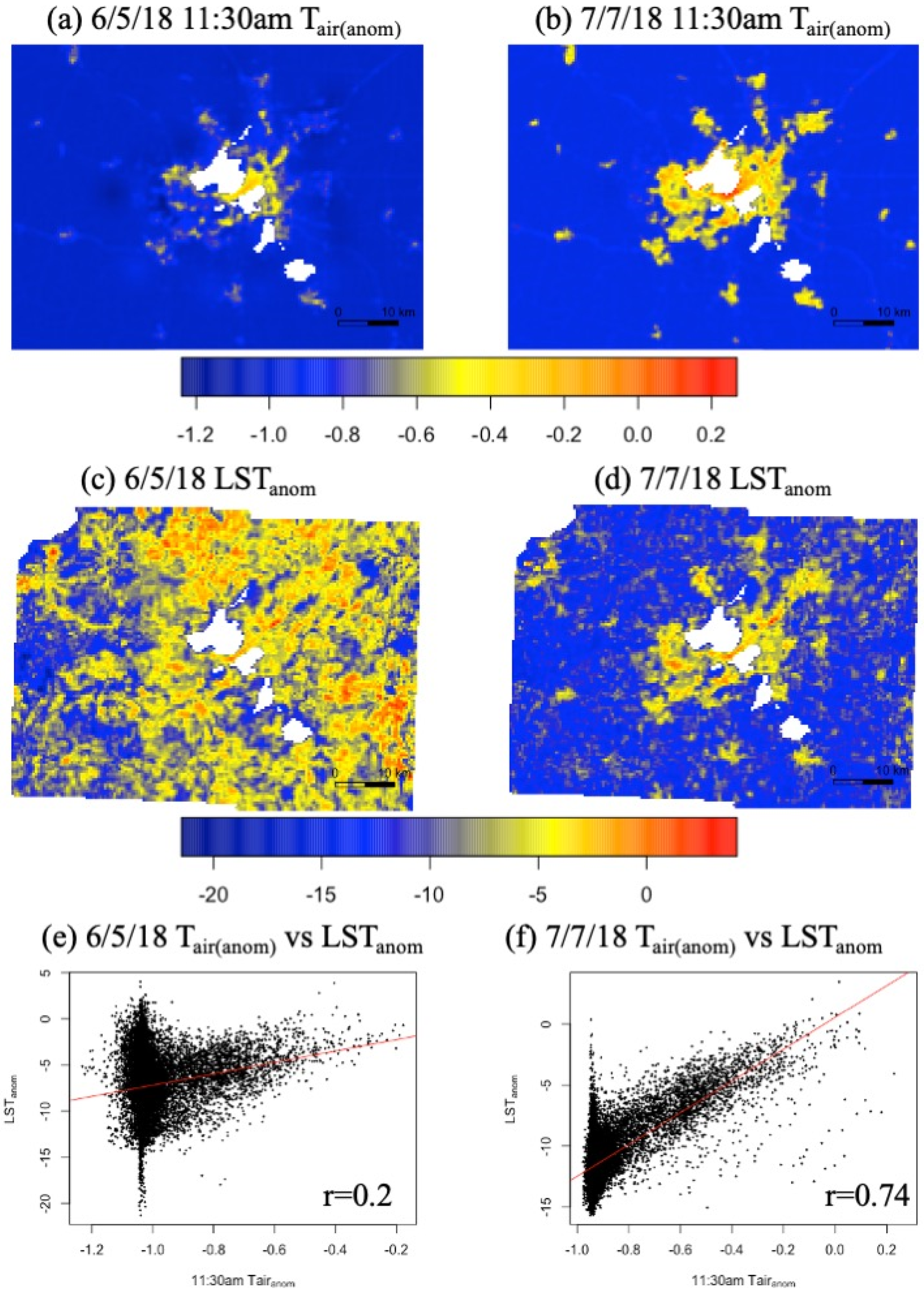
3.2. Comparisons between Individual Dates

A wide range of statistically significant (p < 0.001) correlations between Tair(anom) and LSTanom were found over all 15 individual dates studied (Table 3). Although the same analysis was conducted for all 15 dates, Figure 4 highlights just two dates—5 and 7 July 2018—that display the two extremes observed, despite occurring roughly one month apart. The spatial patterns of 11:30 a.m. Tair(anom) (Figure 4a,b) were more similar across both dates (r = 0.95), than the spatial patterns of LSTanom (r = 0.45). The clear SUHI pattern visible on 7 July (Figure 4d) was absent on 5 June (Figure 4c). Instead, hot and cold patches were scattered throughout urban and rural areas of Dane County. Overall, RMSE between LSTanom and 11:30 a.m. Tair(anom) was higher on 7 July 2018 (10.06 °C) than on 5 June 2018 (6.21 °C).
On both 5 and 7 July 2018, the scatterplot between 11:30 a.m. Tair(anom) and LSTanom displays an artifact of the regression kriging; rural points that shared the same covariate values and were all substantial distances from the sensor network all share the same predicted Tair despite differing in LST, producing the vertical lines seen in Figure 4e,f. This artifact does not obscure the fact that there was a stronger linear relationship between 11:30 a.m. Tair(anom) and LSTanom on 7 July 2018 than there was one month earlier. The pattern of lower correlation on 5 June 2018 and higher correlation on 7 July 2018 was not limited to the comparison between LSTanom and 11:30 a.m. Tair(anom). This trend was also evident in comparisons between day and night Tair(anom). On 6–7 July, the correlation between 11:30 a.m. and 11:30 p.m. Tair(anom) was 0.79, while the same comparison for the 4–5 June scene had an r-value of just 0.37.
Although results from only two dates are depicted in Figure 4, all 15 dates displayed similar trends. Dates with low correlation between LSTanom and 11:30 a.m. Tair(anom) typically had low RMSE values as well. Figure 5a shows a positive linear trend between these two statistical metrics (R2 = 0.54, p = 0.002). Overall, on days when the spatial distribution of LSTanom most closely resembled the spatial distribution of 11:30 a.m. Tair(anom), the magnitude of the differences between these anomalies was also at its largest. No linear trend (R2 = 0.0003, p = 0.95) was present between these metrics for the 11:30 p.m. Tair(anom) and 11:30 a.m. Tair(anom) comparison (Figure 5b). The impact of wind speed and daily high and low temperatures on RMSE and correlation coefficient was also explored, but no relationship was found.

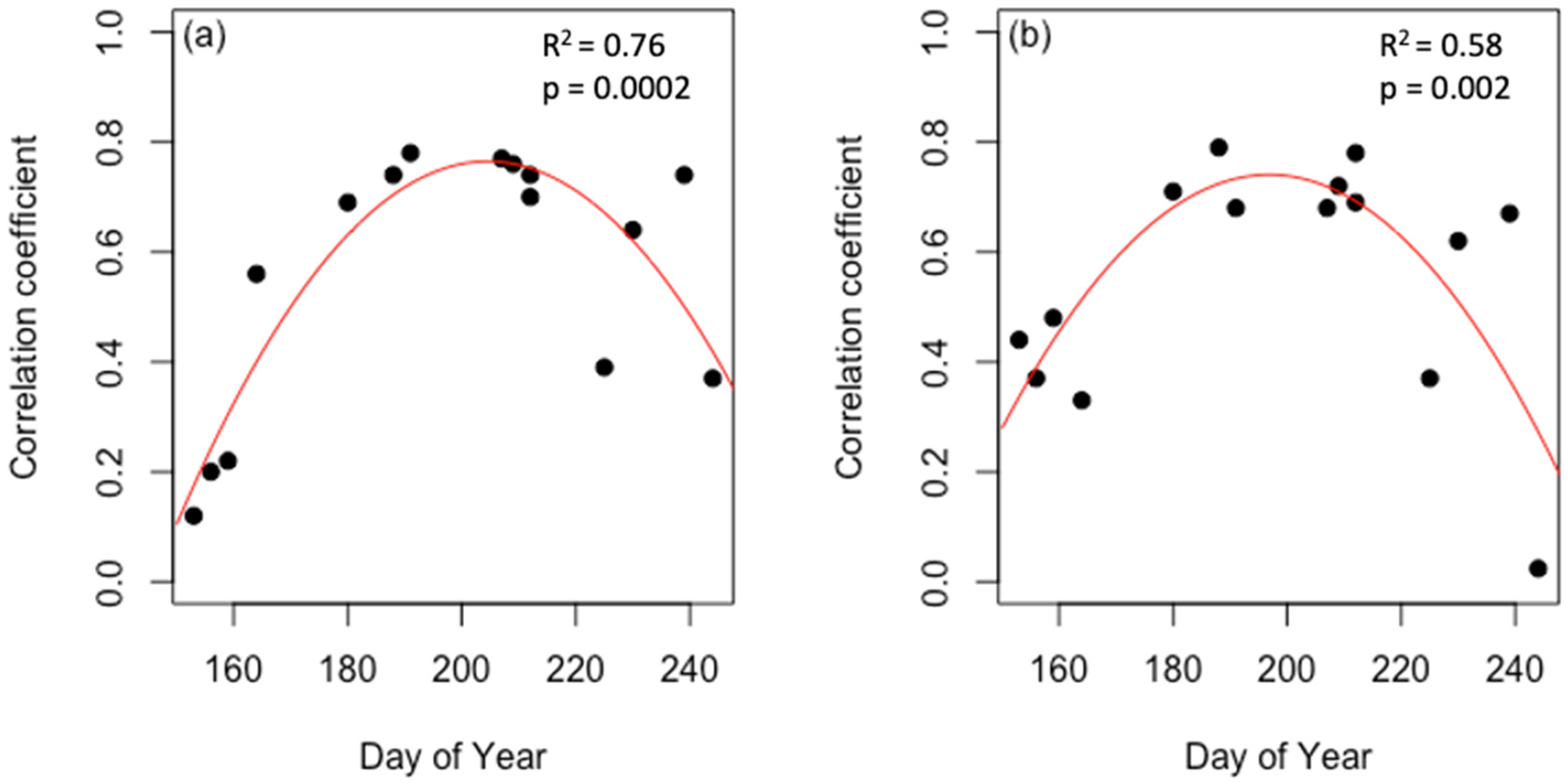
3.3. Trends by Day of Year

Correlation between LST and 11:30 a.m. Tair was lowest at the beginning and end of the summer, peaking in late July. Some summer weeks were represented more frequently than others; for example, four scenes from the last week of July were included, but no scenes between 14 and 28 June or between 1 and 12 August were suitable for analysis. Despite these gaps, a parabolic curve (R2 = 0.76, p = 0.0002) was fit to the relationship between the day of the year and the correlation between LSTanom and 11:30 a.m. Tair(anom) (Figure 6a). The correlation coefficient between 11:30 a.m. Tair(anom) and 11:30 p.m. Tair(anom) also followed a parabolic curve when plotted against the day of the year (Figure 6b), but the fit was weaker (R2 = 0.58, p = 0.002).

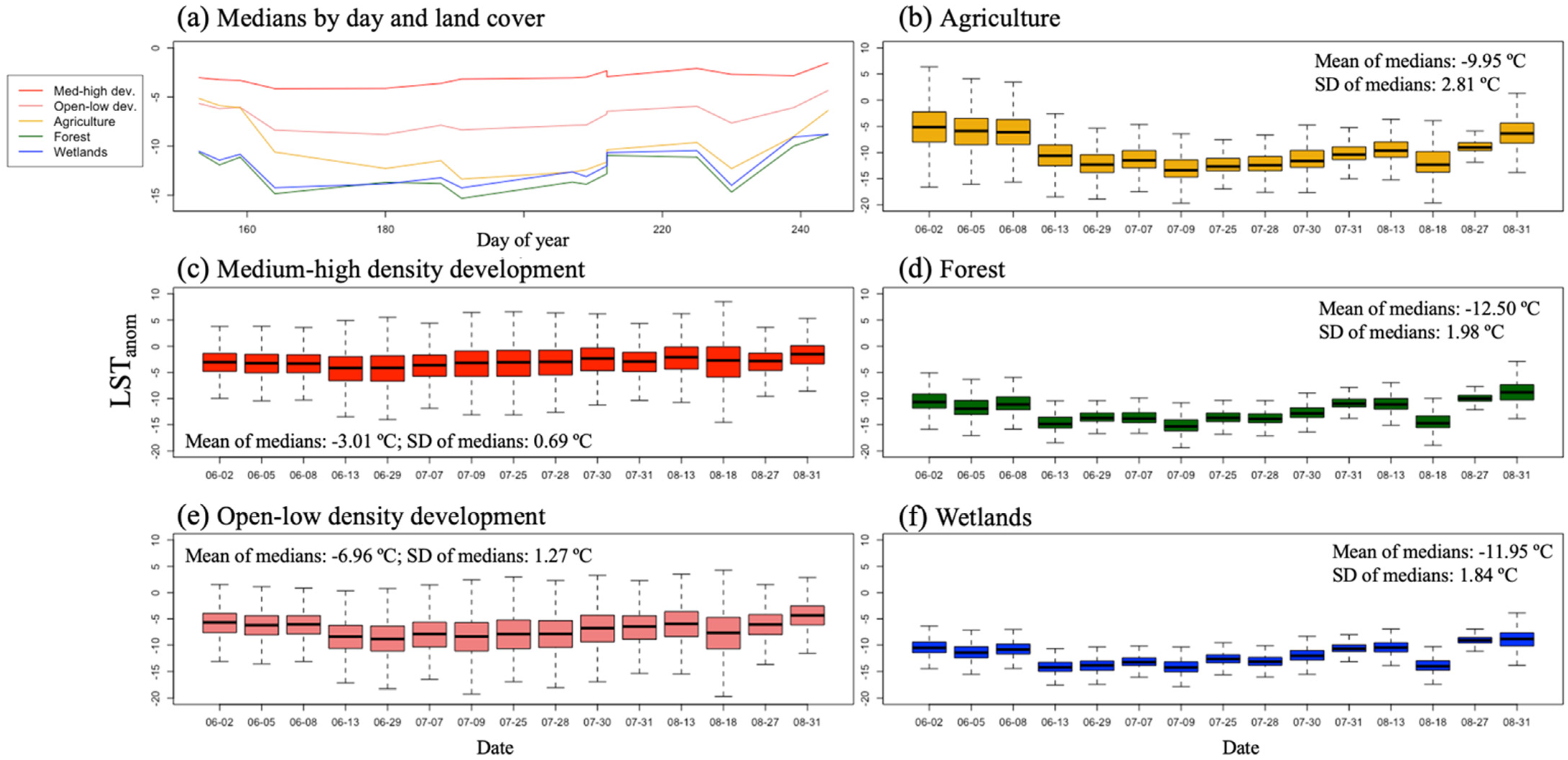
3.4. Impacts of Land Cover

Although the spatial patterns of the Tair-based UHI were quite similar over all 15 dates, the shape and intensity of the SUHI varied greatly between days. Grouping LSTanom by land cover shows that this variability in LST was greater for some land uses than for others (p < 0.001). Both lower and higher intensity development, for example, displayed low variability in LSTanom across all 15 dates, and the standard deviation of the median pixel in these two categories was just 0.69 °C and 1.27 °C, respectively (Figure 7c,e). Forests and wetlands both displayed slightly greater variability, with standard deviations of 1.98 °C and 1.84 °C, respectively (Figure 7d,f). In contrast, median LSTanom values across all agricultural land in Dane County was highly variable, with a maximum value of −5.14 °C on 2 June 2017, a minimum value of −13.37 °C on 9 July 2016, and an overall standard deviation of 2.81 °C, 0.83 °C higher than the next most variable category (Figure 7b). The variance across all fifteen days was higher for agriculture than for medium-high density development (p < 0.001) or for open-low density development (p = 0.003), but there was no statistically significant difference between the variance for agricultural and forested land (p = 0.101) or between agriculture and wetlands (p = 0.063). In addition to the relatively high standard deviation in median LSTanom for agriculture, the spread of LSTanom was also more variable for agriculture than any other land cover class. The interquartile range of LSTanom for agriculture was largest early in the season, with an average value of 4.59 °C across all five June dates. Across six July dates and four August dates, the agricultural interquartile ranges fell to 2.91 °C and 3.04 °C, respectively. No other land cover categories demonstrated such variability in spread; the interquartile range was consistently large for the two developed classes and narrow for the two other vegetated classes.
Over all 15 days, LST was consistently lowest for forest and wetland pixels and highest for medium- to high-density development. Lower intensity development was the second warmest category on every date other than 2 June 2017. On most days, median agricultural LSTanom was higher than the other two vegetated classes and lower than the two developed land categories, but the difference between agricultural LST and the four other land cover classes shifted throughout the summer season. Across the three early June dates, median LSTanom for agriculture fell within 1 °C of the median for open-low development, while over the latter half of the summer, median LSTanom values across agricultural land were closer to the medians for forest and wetland pixels than to the developed land categories (Figure 7a).

4. Discussion

4.1. Increased Understanding of the UHI in a Mid-Sized Midwestern City

This study expanded upon past work using an observation network in Madison, Wisconsin to study the region’s urban climate. By evaluating a longer period of record and incorporating two different measures of temperature, our results simultaneously support past findings and allow for a more nuanced look at Madison’s urban climatology. An analysis of the first 20 months of sensor data (spanning two summers, including the historically warm summer of 2012) found that the Tair-based UHI was largest in August when it averaged 1.5 °C during the day and 4 °C at night [13]. Our analysis used a different methodology, evaluated fewer dates, and spanned a longer temporal range, yet we produced similar results. A 2014 analysis of the first year of Madison sensor network data identified a positive correlation between temperature and density of development and a visible distinction between land within Madison city limits, which experienced urban warming, and rural Dane County, where air temperatures were consistently lower [13]. We find these same spatial patterns in all eight summers of our own Tair analysis. For the first time, we show that these same patterns were also visible in summertime LSTanom. Our results offer new insight into the impact that the rural portions of the county have on regional UHI trends. We showed that high variability in agricultural LSTanom may drive variability in the relationship between LST and Tair.
Instead of comparing urban temperatures to a rural reference point, we compared temperatures to those recorded at central downtown sensors, essentially quantifying rural cooling instead of urban warming. This methodology avoids the ambiguity of identifying an appropriate rural reference. Past studies have shown that slight differences between chosen rural reference points can greatly impact the calculated UHI magnitude, making it difficult to compare UHIs between cities [52,53,57]. Our research highlights an additional concern; because rural LSTanom was so variable, defining the UHI in reference to rural locations would restrict temperature anomaly comparisons across dates. Given the ubiquity of satellite data in UHI studies, the results seen here are worth considering more broadly. This finding is likely most relevant for other Midwestern cities, particularly those with mid-sized populations. We believe that the observed variability in rural LST is tied to Madison’s heavily agricultural rural surroundings, which resembles the landscape that also surrounds many similarly-sized Midwestern cities.

4.2. Impacts of Plant Phenology on the SUHI

Previous research on urban phenology has found that UHIs can lengthen the growing season and shape growth characteristics as far as 15 km outside of cities [58,59,60,61]. Midwestern agriculture has been observed to impact the regional climate by reducing daytime high temperatures [62,63]. The impact of agricultural phenology on temperature differences across urban, peri-urban, and rural climates, however, has been less widely explored [64]. Across 15 summer dates between 2012 and 2019, we found a strong parabolic relationship between the correlation coefficient and day of the year (Figure 6), while meteorological factors (Table 1) did not have a noticeable impact on the relationship between Tair(anom) and Tair(anom). These results, combined with the high variability in LSTanom across agricultural land (Figure 7), suggest plant phenology as a key driver of the changing relationship between Tair(anom) and LSTanom in Dane County.
Agricultural lands surrounding Madison experience significant changes in LST throughout the growing season. The growing season in this region typically begins in early to mid-May and ends in early to mid-October [58]. During the intervening months, the rural landscape changes dramatically. Satellite imagery of agricultural land across Wisconsin shows that statewide corn emergence typically begins between late April and early May [65]. Rapid corn development and growth continue through July when maximum leaf area index (LAI)---the ratio of leaf surface area to ground surface area---is reached, before shifting to the grain fill stage. The emergence of soybeans typically occurs from mid-May and follows a rapid growth and development cycle through July [65].
We hypothesize that spatial heterogeneity in the rural landscape in early June, when some fields are bare soil and others have started to green but still have low LAI, explains the higher and more variable LSTanom observed during these weeks (Figure 7). Low correlation during late summer may indicate senescence, while peak correlation observed near the end of July occurs when Dane County cropland is reaching maximum LAI and biomass [13]. These trends suggest that uniformly green fields and reduced bare soil area contribute to the cooler and narrower range of LSTanom across agricultural land in late July.
Future research could incorporate additional agricultural data to further our understanding of how crop type, phenological development, and crop management decisions impact LST. Our definition of agricultural land use considered all varieties of cultivated crops and pasture as a single category. Past research shows that LST can vary greatly by crop type [66]. Data sources like the USDA’s Cropland Data Layer [67] could aid analysis of how specific crops cool the landscape. Differences in management practices, soil characteristics, and plant health can also differentiate the thermal signature between plants of the same species [66]. Different tillage practices, for example, result in varying levels of residue cover and soil surface roughness, changing the surface energy balance [68]. In Dane County, 30% of farms practice no-till agriculture, and 20% use intensive tillage, potentially contributing to the observed irregularities in early season LSTanom (USDA 2017). Soil moisture is also linked to LST, suggesting that LSTanom at the beginning and end of the growing season, when bare soil cover is greatest, may be driven by drought and moisture conditions [69]. The two dates with the greatest deviations from the parabolic relationship between day of year and correlation (Figure 6a) were both in late summer (27 August 2019 and 13 August 2014). Future investigation of soil moisture conditions and crop senescence during these periods may help explain these two outliers. Additionally, future work could improve our understanding of how agriculture shapes the SUHI by expanding the months of study to include the entire growing season, from spring planting through fall harvest.

4.3. Study Limitations and Future Work

Stationary sensor networks with the size and density seen in Madison, Wisconsin are rare, while satellite measures of LST are widely accessible. As a result, satellite data will continue to be a common data source used in UHI studies, and the relationship between Tair and LST has become an increasingly important question. Our comparison between the air and surface UHIs in Dane County contributes to previous explorations of this research question, but it is important to acknowledge the limitations of this study. Although our sensor array is among the largest urban networks in the world, the number and placement of the temperature sensors are still more limited than the resolution offered by the USGS ARD surface temperature product [13]. Therefore, to enable comparison with the interpolated Tair data, the resolution of the LST files was reduced from 30 m to 400 m. In addition to the lower level of spatial detail offered by this coarser resolution, this resampling and aggregation process introduces errors to each pixel value, on top of the 2.2–2.3 °C land pixel error in the raw ARD data files [40,46,47]. Our study was further limited by the range of meteorological conditions present during the 15 dates studied. Past research in homogeneous rural settings has identified cloud cover and wind speed as meteorological factors that impact the strength of the relationship between Tair and LST [23,24]. We did not identify any impact of wind speed on the relationship between Tair and LST and were unable to explore the impact of cloud cover due to concerns about satellite image quality under cloudy conditions.
Despite these limitations, our results were generally consistent with similar studies that compared LST-based and Tair-based measures of UHI in other urban settings. LST typically exhibits a greater temperature range than measurements of Tair in the same locations [32]. Due to this difference in temperature range, LST and Tair are generally poorly correlated [20,32], but their spatial distributions may display greater similarities [14,33]. Our results support these conclusions; on all 15 dates studied, the range in LSTanom was always greater than the range in Tair(anom), and the average correlation in spatial patterns between LSTanom and Tair(anom) was relatively high, both during the day and at night. Overall, in Madison, and potentially other comparable cities, the SUHI appears to reflect the Tair-based UHI most accurately in late July, during the peak of the growing season. This is a useful finding; however, the ability to model Tair from LST would make urban satellite data even more valuable.
Several past studies have attempted to predict Tair from LST in specific locations, typically employing statistical regressions, relying on empirical relationships between vegetation indices and temperature, or using models of surface energy balance [11,70,71,72,73]. These models commonly produce estimates of Tair at relatively coarse spatial resolutions, limited both by the availability of widespread ground stations for validation and the 1-km resolution of the MODIS sensors and have been found to produce errors of 1 to 3 °C [11,70,71,72,73]. This task is still typically described as an open challenge [18,74]. With more than eight years of spatially-rich air temperature data available for model testing, future research can potentially use the LST and Tair patterns observed in this analysis to produce a methodology for predicting Dane County air temperatures from satellite data.

5. Conclusions

As urban populations continue to grow, it is essential to understand the unique climatic patterns and risks posed by development. The mechanisms of urban warming are widely understood and have been observed in cities around the world, but data sources used to monitor UHIs are often imperfect. Stations that measure Tair can accurately record nearby meteorological conditions but only provide limited spatial coverage. In comparison, satellites measure LST over large swaths of land at once, but these scenes only reflect a single moment in time. Beyond these spatial and temporal concerns, the applicability of the SUHI to the lived experience of urban populations is unclear. Given these concerns, our research combined two rich sources of temperature data in Dane County, Wisconsin—a network of 150 stationary Tair sensors and a 30-m resolution Landsat surface temperature product—to better understand how Tair and LST relate to each other, as well as if and when remote sensing data accurately reflect conditions of urban warming.
Overall, we found that although the magnitude of LST and Tair anomalies differ greatly, these different measures of temperature display similar spatial patterns, suggesting that satellite data can be useful for identifying where peak temperatures occur. Additionally, our analysis suggests that the relationship between Tair and LST changes as the growing season progresses; our data exhibited a maximum correlation during the middle of the summer when the rural, agricultural landscapes are more homogeneous and row crops have reached full canopy cover. These results highlight potential challenges in quantifying UHIs in agricultural regions, but they can also inform further exploration of the unique climatology of mid-sized Midwestern cities. With a greater understanding of the relationship between LST and Tair in the region, the historic satellite record can be used to back-cast Tair UHI patterns over recent decades, allowing for analysis of how urban growth and development has shaped the local climate.

Author Contributions

Conceptualization, E.B. and C.K.; methodology, E.B. and C.K.; software, E.B.; validation, E.B.; formal analysis, E.B.; investigation, E.B.; resources, C.K.; data curation, E.B. and C.K.; writing—original draft preparation, E.B.; writing—review and editing, E.B. and C.K.; visualization, E.B.; supervision, C.K.; project administration, C.K.; funding acquisition, C.K. All authors have read and agreed to the published version of the manuscript.

Funding

This research was funded by the National Science Foundation North Temperature Lakes Long-Term Ecological Research (DEB-1440297) program, with additional support from a UW-Madison University Fellowship. Support for this fellowship is provided by the Graduate School, part of the Office of Vice Chancellor for Research and Graduate Education at the University of Wisconsin-Madison, with funding from the Wisconsin Alumni Research Foundation and the UW-Madison.

Data Availability Statement

All Landsat LST data used in this analysis can be accessed with the USGS Earth Explorer tool (https://earthexplorer.usgs.gov/, accessed on 1 September 2019). Air temperature data from the Madison sensor network, along with coordinates of sensor locations (https://doi.org/10.6073/pasta/8f920f4f7c9634889493c4c1f9189981, accessed on 1 December 2021), are available from the North Temperate Lakes---Long-Term Ecological Research database (https://lter.limnology.wisc.edu/data, accessed on 1 December 2021).

Acknowledgments

We thank Ankur Desai and Kurt Paulsen for their helpful suggestions and feedback. We also thank Emily Marrs Heineman for her work to maintain the sensor network and Jason Schatz for sharing his spatial interpolation R code. Lastly, we are grateful to Madison Gas & Electric, Alliant Energy, the City of Madison, Madison City Parks, Sun Prairie Utilities, Waunakee Utilities, the UW-Madison Arboretum, the City of Fitchburg, UW-Madison, and Dane County for allowing the use of their utility poles for our sensor network.

Conflicts of Interest

The authors declare no conflict of interest.

References

  1. Gao, J.; O’Neill, B.C. Mapping global urban land for the 21st century with data-driven simulations and Shared Socioeconomic Pathways. Nat. Commun. 2020, 11, 2302. [Google Scholar] [CrossRef]
  2. Huang, K.; Li, X.; Liu, X.; Seto, K.C. Projecting global urban land expansion and heat island intensification through 2050. Environ. Res. Lett. 2019, 14, 114037. [Google Scholar] [CrossRef] [Green Version]
  3. Climate Change 2014: Synthesis Report; Intergovernmental Panel on Climate Change: Geneva, Switzerland, 2015.
  4. Weng, Q.; Yang, S. Urban Air Pollution Patterns, Land Use, and Thermal Landscape: An Examination of the Linkage Using GIS. Environ. Monit. Assess. 2006, 117, 463–489. [Google Scholar] [CrossRef] [PubMed]
  5. Schatz, J.; Kucharik, C.J. Urban heat island effects on growing seasons and heating and cooling degree days in Madison, Wisconsin USA. Int. J. Clim. 2016, 36, 4873–4884. [Google Scholar] [CrossRef] [Green Version]
  6. Santamouris, M.; Papanikolaou, N.; Livada, I.; Koronaki, I.; Georgakis, C.; Argiriou, A.; Assimakopoulos, D. On the impact of urban climate on the energy consumption of buildings. Sol. Energy 2001, 70, 201–216. [Google Scholar] [CrossRef]
  7. Patz, J.A.; Campbell-Lendrum, D.; Holloway, T.; Foley, J.A. Impact of regional climate change on human health. Nature 2005, 438, 310–317. [Google Scholar] [CrossRef] [PubMed]
  8. Zhao, L.; Oppenheimer, M.; Zhu, Q.; Baldwin, J.; Ebi, K.L.; Bou-Zeid, E.; Guan, K.; Liu, X. Interactions between urban heat islands and heat waves. Environ. Res. Lett. 2018, 13, 034003. [Google Scholar] [CrossRef]
  9. Broadbent, A.M.; Krayenhoff, E.S.; Georgescu, M. The motley drivers of heat and cold exposure in 21st century US cities. Proc. Natl. Acad. Sci. USA 2020, 117, 21108–21117. [Google Scholar] [CrossRef]
  10. Mirzaei, M.; Verrelst, J.; Arbabi, M.; Shaklabadi, Z.; Lotfizadeh, M. Urban Heat Island Monitoring and Impacts on Citizen’s General Health Status in Isfahan Metropolis: A Remote Sensing and Field Survey Approach. Remote Sens. 2020, 12, 1350. [Google Scholar] [CrossRef]
  11. Pichierri, M.; Bonafoni, S.; Biondi, R. Satellite air temperature estimation for monitoring the canopy layer heat island of Milan. Remote Sens. Environ. 2012, 127, 130–138. [Google Scholar] [CrossRef]
  12. Zhang, F.; Cai, X.; Thornes, J.E. Birmingham’s air and surface urban heat islands associated with Lamb weather types and cloudless anticyclonic conditions. Prog. Phys. Geogr. Earth Environ. 2014, 38, 431–447. [Google Scholar] [CrossRef]
  13. Schatz, J.; Kucharik, C. Seasonality of the Urban Heat Island Effect in Madison, Wisconsin. J. Appl. Meteorol. Clim. 2014, 53, 2371–2386. [Google Scholar] [CrossRef]
  14. Schwarz, N.; Schlink, U.; Franck, U.; Großmann, K. Relationship of land surface and air temperatures and its implications for quantifying urban heat island indicators—An application for the city of Leipzig (Germany). Ecol. Indic. 2012, 18, 693–704. [Google Scholar] [CrossRef]
  15. Ziter, C.D.; Pedersen, E.J.; Kucharik, C.J.; Turner, M.G. Scale-dependent interactions between tree canopy cover and impervious surfaces reduce daytime urban heat during summer. Proc. Natl. Acad. Sci. USA 2019, 116, 7575–7580. [Google Scholar] [CrossRef] [PubMed] [Green Version]
  16. Rajkovich, N.B.; Larsen, L. A Bicycle-Based Field Measurement System for the Study of Thermal Exposure in Cuyahoga County, Ohio, USA. Int. J. Environ. Res. Public Health 2016, 13, 159. [Google Scholar] [CrossRef]
  17. Oke, T.R. City Size and the Urban Heat Island. Atmos. Environ. 1973, 7, 769–779. [Google Scholar] [CrossRef]
  18. Zhou, D.; Xiao, J.; Bonafoni, S.; Berger, C.; Deilami, K.; Zhou, Y.; Frolking, S.; Yao, R.; Qiao, Z.; Sobrino, J.A. Satellite Remote Sensing of Surface Urban Heat Islands: Progress, Challenges, and Perspectives. Remote Sens. 2019, 11, 48. [Google Scholar] [CrossRef] [Green Version]
  19. Rao, P.K. Remote Sensing of Urban “Heat Islands” from an Environmental Satellite. Bull. Am. Meteorol. Soc. 1972, 53, 647–648. [Google Scholar]
  20. Voogt, J.A.; Oke, T.R. Thermal remote sensing of urban climates. Remote Sens. Environ. 2003, 86, 370–384. [Google Scholar] [CrossRef]
  21. Imhoff, M.L.; Zhang, P.; Wolfe, R.E.; Bounoua, L. Remote sensing of the urban heat island effect across biomes in the continental USA. Remote Sens. Environ. 2010, 114, 504–513. [Google Scholar] [CrossRef] [Green Version]
  22. White-Newsome, J.L.; Brines, S.J.; Brown, D.G.; Dvonch, J.T.; Gronlund, C.J.; Zhang, K.; Oswald, E.M.; O’Neill, M.S. Validating Satellite-Derived Land Surface Temperature within SituMeasurements: A Public Health Perspective. Environ. Health Perspect. 2013, 121, 925–931. [Google Scholar] [CrossRef] [Green Version]
  23. Gallo, K.; Hale, R.; Tarpley, D.; Yu, Y. Evaluation of the Relationship between Air and Land Surface Temperature under Clear- and Cloudy-Sky Conditions. J. Appl. Meteorol. Clim. 2011, 50, 767–775. [Google Scholar] [CrossRef]
  24. Good, E.J. An in situ-based analysis of the relationship between land surface “skin” and screen-level air temperatures. J. Geophys. Res. Atmos. 2016, 121, 8801–8819. [Google Scholar] [CrossRef]
  25. Kawashima, S.; Ishida, T.; Minomura, M.; Miwa, T. Relations between Surface Temperature and Air Temperature on a Local Scale during Winter Nights. J. Appl. Meteorol. 2000, 39, 1570–1579. [Google Scholar] [CrossRef]
  26. Mutiibwa, D.; Strachan, S.; Albright, T. Land Surface Temperature and Surface Air Temperature in Complex Terrain. IEEE J. Sel. Top. Appl. Earth Obs. Remote Sens. 2015, 8, 4762–4774. [Google Scholar] [CrossRef]
  27. Sohrabinia, M.; Zawar-Reza, P.; Rack, W. Spatio-temporal analysis of the relationship between LST from MODIS and air temperature in New Zealand. Arch. Meteorol. Geophys. Bioclimatol. Ser. B 2014, 119, 567–583. [Google Scholar] [CrossRef]
  28. Zhang, P.; Bounoua, L.; Imhoff, M.L.; Wolfe, R.E.; Thome, K. Comparison of MODIS Land Surface Temperature and Air Temperature over the Continental USA Meteorological Stations. Can. J. Remote Sens. 2014, 40, 15. [Google Scholar] [CrossRef]
  29. Egorov, A.V.; Roy, D.P.; Zhang, H.K.; Li, Z.; Yan, L.; Huang, H. Landsat 4, 5 and 7 (1982 to 2017) Analysis Ready Data (ARD) Observation Coverage over the Conterminous United States and Implications for Terrestrial Monitoring. Remote Sens. 2019, 11, 447. [Google Scholar] [CrossRef] [Green Version]
  30. Anniballe, R.; Bonafoni, S.; Pichierri, M. Spatial and temporal trends of the surface and air heat island over Milan using MODIS data. Remote Sens. Environ. 2014, 150, 163–171. [Google Scholar] [CrossRef]
  31. Yoo, C.; Im, J.; Park, S.; Quackenbush, L.J. Estimation of daily maximum and minimum air temperatures in urban landscapes using MODIS time series satellite data. ISPRS J. Photogramm. Remote Sens. 2018, 137, 149–162. [Google Scholar] [CrossRef]
  32. Arnfield, A.J. Two decades of urban climate research: A review of turbulence, exchanges of energy and water, and the urban heat island. Int. J. Clim. 2003, 23, 1–26. [Google Scholar] [CrossRef]
  33. Ho, H.C.; Knudby, A.; Xu, Y.; Hodul, M.; Aminipouri, M. A comparison of urban heat islands mapped using skin temperature, air temperature, and apparent temperature (Humidex), for the greater Vancouver area. Sci. Total Environ. 2016, 544, 929–938. [Google Scholar] [CrossRef]
  34. Sheng, L.; Tang, X.; You, H.; Gu, Q.; Hu, H. Comparison of the urban heat island intensity quantified by using air temperature and Landsat land surface temperature in Hangzhou, China. Ecol. Indic. 2016, 72, 738–746. [Google Scholar] [CrossRef]
  35. Azevedo, J.A.; Chapman, L.; Muller, C.L. Quantifying the Daytime and Night-Time Urban Heat Island in Birmingham, UK: A Comparison of Satellite Derived Land Surface Temperature and High Resolution Air Temperature Observations. Remote Sens. 2016, 8, 153. [Google Scholar] [CrossRef] [Green Version]
  36. Cohen, D.; Hatchard, G.; Wilson, S. Population Trends in Incorporated Places: 2000 to 2013; U.S. Census Bureau: Washington, DC, USA, 2015; p. 19.
  37. U.S. Census Bureau. U.S. Census Bureau QuickFacts: Madison City; Wisconsin: Dane County. Available online: https://www.census.gov/quickfacts/fact/table/madisoncitywisconsin,danecountywisconsin,US/PST045219 (accessed on 15 July 2020).
  38. Schneider, A.; Logan, K.E.; Kucharik, C. Impacts of Urbanization on Ecosystem Goods and Services in the U.S. Corn Belt. Ecosystems 2012, 15, 519–541. [Google Scholar] [CrossRef]
  39. U.S. Department of Agriculture. 2017 Census of Agriculture County Profile: Dane County Wisconsin; U.S. Department of Agriculture: Washington, DC, USA, 2017.
  40. Malakar, N.K.; Hulley, G.C.; Hook, S.J.; Laraby, K.; Cook, M.; Schott, J.R. An Operational Land Surface Temperature Product for Landsat Thermal Data: Methodology and Validation. IEEE Trans. Geosci. Remote Sens. 2018, 56, 5717–5735. [Google Scholar] [CrossRef]
  41. Jiménez-Muñoz, J.C.; Sobrino, J.A. A generalized single-channel method for retrieving land surface temperature from remote sensing data. J. Geophys. Res. Earth Surf. 2003, 108. [Google Scholar] [CrossRef] [Green Version]
  42. Hulley, G.C.; Hook, S.J.; Abbott, E.; Malakar, N.; Islam, T.; Abrams, M. The ASTER Global Emissivity Dataset (ASTER GED): Mapping Earth’s emissivity at 100-m spatial scale. Geophys. Res. Lett. 2015, 42, 7966–7976. [Google Scholar] [CrossRef]
  43. Cook, M.; Schott, J.R.; Mandel, J.; Raqueno, N. Development of an Operational Calibration Methodology for the Landsat Thermal Data Archive and Initial Testing of the Atmospheric Compensation Component of a Land Surface Temperature (LST) Product from the Archive. Remote Sens. 2014, 6, 11244–11266. [Google Scholar] [CrossRef] [Green Version]
  44. Dwyer, J.L.; Roy, D.P.; Sauer, B.; Jenkerson, C.B.; Zhang, H.K.; Lymburner, L. Analysis Ready Data: Enabling Analysis of the Landsat Archive. Remote Sens. 2018, 10, 1363. [Google Scholar] [CrossRef]
  45. Hijmans, R.J. Raster: Geographic Data Analysis and Modeling. 2020. Available online: https://cran.r-project.org/web/packages/raster/raster.pdf (accessed on 20 October 2021).
  46. He, H.S.; Ventura, S.J.; Mladenoff, D.J. Effects of spatial aggregation approaches on classified satellite imagery. Int. J. Geogr. Inf. Sci. 2002, 16, 93–109. [Google Scholar] [CrossRef]
  47. Colin, B.; Schmidt, M.; Clifford, S.; Woodley, A.; Mengersen, K. Influence of Spatial Aggregation on Prediction Accuracy of Green Vegetation Using Boosted Regression Trees. Remote Sens. 2018, 10, 1260. [Google Scholar] [CrossRef] [Green Version]
  48. Good, E.J.; Ghent, D.J.; Bulgin, C.E.; Remedios, J.J. A Spatiotemporal Analysis of the Relationship between Near-Surface Air Temperature and Satellite Land Surface Temperatures Using 17 Years of Data from the ATSR Series. J. Geophys. Res. Atmos. 2017, 4, 2131–2154. [Google Scholar] [CrossRef]
  49. Szymanowski, M.; Kryza, M. Local regression models for spatial interpolation of urban heat island—an example from Wrocław, SW Poland. Theor. Appl. Clim. 2011, 108, 53–71. [Google Scholar] [CrossRef] [Green Version]
  50. Wickham, J.; Homer, C.; Vogelmann, J.; McKerrow, A.; Mueller, R.; Herold, N.; Coulston, J. The Multi-Resolution Land Characteristics (MRLC) Consortium—20 Years of Development and Integration of USA National Land Cover Data. Remote Sens. 2014, 6, 7424–7441. [Google Scholar] [CrossRef] [Green Version]
  51. Lark, T.J.; Mueller, R.M.; Johnson, D.M.; Gibbs, H.K. Measuring land-use and land-cover change using the U.S. department of agriculture’s cropland data layer: Cautions and recommendations. Int. J. Appl. Earth Obs. Geoinf. 2017, 62, 224–235. [Google Scholar] [CrossRef]
  52. Stewart, I.D.; Oke, T.R. Local Climate Zones for Urban Temperature Studies. Bull. Am. Meteorol. Soc. 2012, 93, 1879–1900. [Google Scholar] [CrossRef]
  53. Schwarz, N.; Lautenbach, S.; Seppelt, R. Exploring indicators for quantifying surface urban heat islands of European cities with MODIS land surface temperatures. Remote Sens. Environ. 2011, 115, 3175–3186. [Google Scholar] [CrossRef]
  54. Schatz, J.; Kucharik, C. Urban climate effects on extreme temperatures in Madison, Wisconsin, USA. Environ. Res. Lett. 2015, 10, 094024. [Google Scholar] [CrossRef] [Green Version]
  55. R Core Team. R: A Language and Environment for Statistical Computing. Available online: https://www.R-project.org/ (accessed on 20 December 2021).
  56. Bivand, R.; Keitt, T.; Rowlingson, B.; Pebesma, E.; Sumner, M.; Hijmans, R.; Rouault, E.; Warmerdam, F.; Ooms, J.; Rundel, C. rgdal: Bindings for the “Geospatial” Data Abstraction Library. 2020. Available online: https://cran.r-project.org/web/packages/rgdal/index.html (accessed on 20 October 2021).
  57. Yao, R.; Wang, L.; Huang, X.; Niu, Y.; Chen, Y.; Niu, Z. The influence of different data and method on estimating the surface urban heat island intensity. Ecol. Indic. 2018, 89, 45–55. [Google Scholar] [CrossRef]
  58. Zipper, S.C.; Schatz, J.; Singh, A.; Kucharik, C.J.; Townsend, P.A.; Ii, S.P.L. Urban heat island impacts on plant phenology: Intra-urban variability and response to land cover. Environ. Res. Lett. 2016, 11, 054023. [Google Scholar] [CrossRef]
  59. Melaas, E.K.; Wang, J.; Miller, D.; Friedl, M. Interactions between urban vegetation and surface urban heat islands: A case study in the Boston metropolitan region. Environ. Res. Lett. 2016, 11, 054020. [Google Scholar] [CrossRef] [Green Version]
  60. Villalobos-Jiménez, G.; Hassall, C. Effects of the urban heat island on the phenology of Odonata in London, UK. Int. J. Biometeorol. 2017, 61, 1337–1346. [Google Scholar] [CrossRef] [PubMed] [Green Version]
  61. Zhang, X.; Friedl, M.A.; Schaaf, C.; Strahler, A.H.; Schneider, A. The footprint of urban climates on vegetation phenology. Geophys. Res. Lett. 2004, 31. [Google Scholar] [CrossRef]
  62. Mueller, N.D.; Butler, E.E.; McKinnon, K.; Rhines, A.; Tingley, M.; Holbrook, N.M.; Huybers, P. Cooling of US Midwest summer temperature extremes from cropland intensification. Nat. Clim. Chang. 2015, 6, 317–322. [Google Scholar] [CrossRef] [Green Version]
  63. Nocco, M.A.; Smail, R.A.; Kucharik, C.J. Observation of irrigation-induced climate change in the Midwest United States. Glob. Chang. Biol. 2019, 25, 3472–3484. [Google Scholar] [CrossRef] [PubMed]
  64. Polydoros, A.; Cartalis, C. Assessing the impact of urban expansion to the state of thermal environment of peri-urban areas using indices. Urban Clim. 2015, 14, 166–175. [Google Scholar] [CrossRef]
  65. Zhang, X.; Liu, L.; Henebry, G. Impacts of land cover and land use change on long-term trend of land surface phenology: A case study in agricultural ecosystems. Environ. Res. Lett. 2019, 14, 044020. [Google Scholar] [CrossRef] [Green Version]
  66. Shivers, S.W.; Roberts, D.A.; McFadden, J.P. Using paired thermal and hyperspectral aerial imagery to quantify land surface temperature variability and assess crop stress within California orchards. Remote Sens. Environ. 2019, 222, 215–231. [Google Scholar] [CrossRef]
  67. Boryan, C.; Yang, Z.; Mueller, R.; Craig, M. Monitoring US agriculture: The US Department of Agriculture, National Agricultural Statistics Service, Cropland Data Layer Program. Geocarto Int. 2011, 26, 341–358. [Google Scholar] [CrossRef]
  68. O’Brien, P.L.; Daigh, A.L. Tillage practices alter the surface energy balance—A review. Soil Tillage Res. 2019, 195. [Google Scholar] [CrossRef]
  69. Idso, S.B.; Schmugge, T.J.; Jackson, R.D.; Reginato, R.J. The utility of surface temperature measurements for the remote sensing of surface soil water status. J. Geophys. Res. Earth Surf. 1975, 80, 3044–3049. [Google Scholar] [CrossRef]
  70. Zeng, L.; Wardlow, B.D.; Tadesse, T.; Shan, J.; Hayes, M.J.; Li, D.; Xiang, D. Estimation of Daily Air Temperature Based on MODIS Land Surface Temperature Products over the Corn Belt in the US. Remote Sens. 2015, 7, 951–970. [Google Scholar] [CrossRef] [Green Version]
  71. Li, L.; Huang, X.; Li, J.; Wen, D. Quantifying the Spatiotemporal Trends of Canopy Layer Heat Island (CLHI) and Its Driving Factors over Wuhan, China with Satellite Remote Sensing. Remote Sens. 2017, 9, 536. [Google Scholar] [CrossRef] [Green Version]
  72. Li, X.; Zhou, Y.; Asrar, G.R.; Zhu, Z. Developing a 1 km resolution daily air temperature dataset for urban and surrounding areas in the conterminous United States. Remote Sens. Environ. 2018, 215, 74–84. [Google Scholar] [CrossRef]
  73. Huang, W.; Li, J.; Guo, Q.; Mansaray, L.R.; Li, X.; Huang, J. A Satellite-Derived Climatological Analysis of Urban Heat Island over Shanghai during 2000–2013. Remote Sens. 2017, 9, 641. [Google Scholar] [CrossRef] [Green Version]
  74. Weng, Q. Thermal infrared remote sensing for urban climate and environmental studies: Methods, applications, and trends. ISPRS J. Photogramm. Remote Sens. 2009, 64, 335–344. [Google Scholar] [CrossRef]
Figure 1. Maps of land cover over (a) the entire study area (Dane County, Wisconsin), and (b) downtown Madison. Locations of all stationary air temperature/relative humidity sensors are indicated with black dots. Green markers indicate the locations of the five sensors used as central reference points.
Remotesensing 14 00165 g001
Figure 2. (a) LST, (b) 11:30 a.m. Tair, and (c) 11:30 p.m. Tair anomalies at 400-m resolution, averaged over the 15 dates studied. Temperatures of the lakes (in white) are masked out.
Remotesensing 14 00165 g002
Figure 3. The absolute magnitude of the difference between LSTanom and Tair(anom) by time of day, averaged over all 15 dates of study across (a) all pixels, (b) all urban pixels, and (c) all rural pixels. Urban pixels are all those categorized as higher and lower density development, and rural pixels are all those categorized as forest, agriculture, grasslands, barren, or wetlands.
Remotesensing 14 00165 g003
Figure 4. (a,b) Tair(anom) and (c,d) LSTanom for two different dates during summer 2018. (e,f) show scatterplots of Tair(anom) plotted against LSTanom. All panels in the left column display data from 5 June 2018 and panels in the right column displays data from 7 July 2018. Temperatures of the lakes (in white) are masked out from (a) through (d).
Remotesensing 14 00165 g004
Figure 5. RMSE plotted against correlation coefficient for (a) the relationship between LSTanom and 11:30 a.m. Tair(anom) and (b) the relationship between 11:30 p.m. Tair(anom) and 11:30 a.m. Tair(anom).
Remotesensing 14 00165 g005
Figure 6. Correlation coefficient plotted against the day of the year for (a) the relationship between LSTanom and 11:30 a.m. Tair(anom) and (b) the relationship between 11:30 p.m. Tair(anom) and 11:30 a.m. Tair(anom).
Remotesensing 14 00165 g006
Figure 7. (a) Dane County median LSTanom by day of year across five land cover categories and (bf) boxplots of LSTanom by date for each individual category. Each box plot indicates the interquartile range (IQR), with the edges marking the first (Q1) and third (Q3) quartiles, the central black line indicating the medians, and the upper and lower whiskers indicating the LSTanom values equal to Q3 + 1.5 * IQR and Q1 − 1.5 * IQR, respectively.
Remotesensing 14 00165 g007
Table 1. Dates, satellite, daily high and low air temperatures, and daily mean and maximum wind speed for the 15 scenes analyzed. Daily temperature data and wind speed were recorded at the Dane County Regional Airport and accessed through the Midwestern Regional Climate Center’s online data portal.
DateSatelliteTmax (°C)Tmin (°C)Mean Wind Speed (m/s)Max Wind Speed (m/s)
7/30/12Landsat 732.218.31.653.58
8/31/12Landsat 732.819.42.595.81
8/18/13Landsat 726.711.11.214.02
8/13/14Landsat 826.712.82.504.92
7/31/15Landsat 827.219.43.266.71
7/9/16Landsat 726.716.12.956.26
7/25/16Landsat 729.419.42.014.47
6/2/17Landsat 827.88.91.393.58
7/28/17Landsat 726.115.64.027.15
6/5/18Landsat 821.711.72.914.92
6/13/18Landsat 726.115.63.006.71
6/29/18Landsat 733.921.74.476.71
7/7/18Landsat 826.110.62.777.15
6/8/19Landsat 827.212.83.138.05
8/27/19Landsat 824.416.12.415.81
Table 2. Original NLCD classes and consolidated land cover categories used in the land cover analysis.
NLCD NumberNLCD NameConsolidated CategoriesPercent of Dane County
11Open WaterWater3.19%
21Developed, Open SpaceLower intensity development11.42%
22Developed, Low Intensity
23Developed, Medium IntensityHigher intensity development3.58%
24Developed, High Intensity
31Barren Land (Rock/Sand/Clay)Bare land0.20%
41Deciduous ForestForest14.48%
42Evergreen Forest
43Mixed Forest
52Shrub/ScrubShrub and grassland0.36%
71Grassland/Herbaceous
81Pasture/HayAgriculture60.21%
82Cultivated Crops
90Woody WetlandsWetland6.57%
95Emergent Herbaceous Wetlands
Table 3. Correlation coefficients between all three measures of temperature and 15 dates studied, arranged by day in the summer season. All of the correlation coefficients in the table are statistically significant (p < 0.001).
Day of YearDateCorrelation Coefficients
11:30 a.m. Tair(anom) vs. LSTanom11:30 p.m. Tair(anom) vs. LSTanom11:30 a.m. Tair(anom) vs. 11:30 p.m. Tair(anom)
1536/2/170.120.240.44
1566/5/180.20.0480.37
1596/8/190.220.280.48
1646/13/180.560.350.33
1806/29/180.690.450.71
1887/7/180.740.580.79
1917/9/160.780.550.68
2077/25/160.770.480.68
2097/28/170.760.720.72
2127/30/120.740.700.78
2127/31/150.70.580.69
2258/13/140.390.400.37
2308/18/130.640.420.62
2398/27/190.740.630.67
2448/31/120.370.180.024
Publisher’s Note: MDPI stays neutral with regard to jurisdictional claims in published maps and institutional affiliations.

