1. Introduction
The Apulian peninsular coastline extends for about 940 km and is made up of 33% sandy beaches (about 320 km), 33% low rocky coasts, 21% high cliffs (about 601 km of non-sandy coast), almost all of which are affected by wave erosion [
1] and 5% anthropized stretches (about 49 km).
Coastal monitoring is an important activity for the protection and preservation of these areas. To achieve this goal, the EEA (European Environment Agency) launched, in 2019, the implementation of a new thematic hotspot product to monitor landscape dynamics in European coastal zones (
https://land.copernicus.eu/local/coastal-zones (accessed on 15 February 2021)). Cliffs and rocky coasts have received less scientific attention than the evolution of the sand coasts [
2]. However, gravity phenomena such as collapses and overturning are the dominant and most visible process in cliff coasts [
3]. These phenomena, generally unexpected, occasional and difficult to predict, are due to the concomitance of various factors (seasonal variations in erosion processes and the interaction between geomechanical and geomorphological factors) [
4]. Therefore, these are certainly difficult aspects to approach in terms of hazard definition. In addition, natural factors are associated with the increasing urbanisation of coastal areas, which has led to cliff instability being an increasingly important problem in many areas [
5].
In the last few years, investigation methodologies have been developed that, starting from the analysis of three-dimensional point cloud models, provide a manual [
6], semi-automatic [
7,
8,
9] and automatic approach to remotely define the structural characteristics of rock groups.
Manual techniques consist of subjectively selecting sub-regions of point clouds assimilated to a single plane of interest by performing orientation measurements using different calculation methods [
10,
11,
12]. Automatic or semi-automatic approaches include the creation of TIN (triangulated irregular network) surfaces and the subsequent automatic identification of the orientation of the normal vector for each polygon generated [
8,
13]. The automatic approach requires a clear definition of the density of the triangles, the maximum angle that can be considered between neighbouring triangles and the minimum size of the triangles [
8], in order to determine whether two adjacent triangular elements should be considered coplanar or uncoplanar [
6]. Other automatic approaches permit point clouds to be divided into sub-cells by identifying elementary planar objects and aggregating them in the function of a predefined threshold [
14].
More sophisticated analysis techniques are based on the definition of surface orientations, based on 3D point clouds only [
9,
15,
16,
17,
18]. The most used and known software tools for analysis are Coltop 3D [
9] and FACETS [
14]. Coltop3D is a software that carries out structural analysis using the digital elevation model (DEM) and 3D point clouds acquired with terrestrial laser scanners and a colour representation combining slope aspect and slope angle is used to obtain a unique colour code for each orientation of a local slope [
19,
20]. FACETS is a dedicated plugin in Cloud Compare free software implemented to perform extraction of planar facets, calculate their Dip/Dip direction and report the extracted data in interactive stereograms. Two algorithms perform the segmentation: Kd-Tree and Fast Marching, both dividing the point cloud into sub-cells, and then calculating elementary planar objects and progressively aggregating these into polygons. One of the great features of FACETS is the ability to explore planar objects, as well as 3D points with their normals, using the stereogram tool [
14].
In the present study, a different approach is taken to the analysis based on the verification of morphological variations in the area under investigation. In particular, the identification of sub-areas is done by choosing only visually similar morphological elements. Through the sub-box analysis, it is possible to detect temporal variations in distances and volumes in the different datasets (3D point cloud). In order to achieve these goals, different algorithms were implemented using in-house software.
1.1. Morphological Structures of Cliffs
The cliff is the consequence of the wave erosion of semi-coherent to coherent rocks, forming a rock face with a high inclination to the sea [
1,
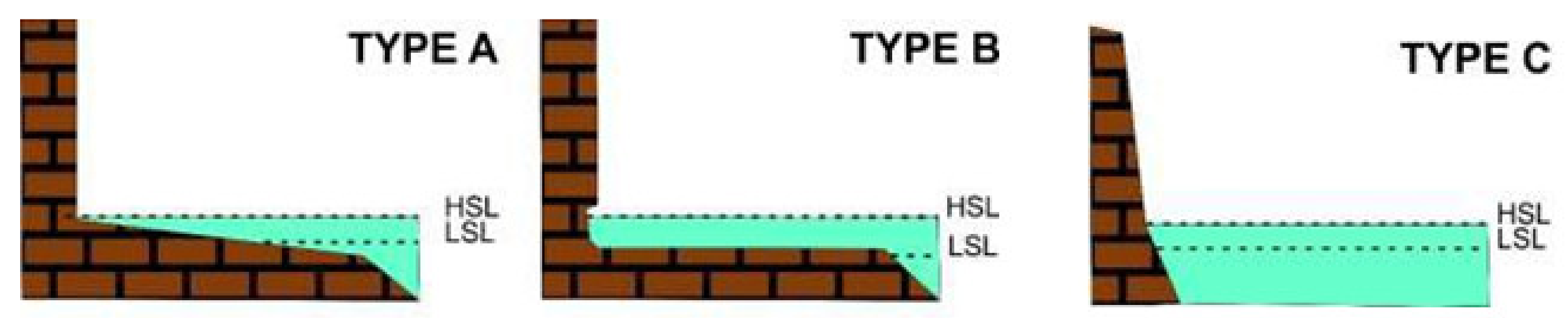
21]. The cliff, as classified by Sunamura [
3,
22], is of three types (
Figure 1):
Type A with a shore platform inclined towards the sea;
Type B with horizontal shore platform;
Type C with plunging cliff.
In type C cliffs, the rock face continues below sea level and, due to its steepness, is able to reflect incident waves without allowing energy to be dissipated by shoaling. These cliffs are generally more stable. Type A and B cliffs are differentiated by the different inclination of the coastal platform before them; according to Sunamura [
22], both are generated by cliff recession, a phenomenon that depends mainly on the relationship between the erosive force of the waves (mechanical and hydraulic) and the durability of the stone materials making up the wall.
An initial interpretation of cliff evolution was given by Sunamura [
3], who defined it as cyclical, where the initial phase of detachment of material from the wall is followed by its transport and deposition. The deposited material, in the form of a slope or beach deposit, acts as a protection for the cliff against the erosive activity of wave motion. The possible removal of the detritus by meteo-marine events then allows the evolution cycle to resume. On these coasts, it is possible to find small beaches (pocket beaches) embedded in the cliffs, enclosed between two promontories jutting out into the sea that prevent or limit the exchange of sediments with the neighbouring coastline [
23]. The shape of the beaches is connected to the direction of the wave motion and to the morphological structure of the promontories that delimit them. Beach deposits are supplied by small hydrographic basins and cliff collapses: both phenomena, in addition to constituting the sedimentary input necessary to maintain the beach “resource”, determine scenarios of high geomorphological hazard.
1.2. Aim of the Work
The aim of the work is to define a methodological approach to monitoring the evolution of such coastal stretches over time. Starting from the acquisition of the morphological structure of the site, through the integration of different geomatic techniques, algorithms dedicated to the identification of instability phenomena were developed in order to ensure a rigorous design of possible risk mitigation works.
The use of the most innovative three-dimensional remote sensing techniques, such as laser scanning and digital photogrammetry (with fixed or mobile acquisition), has shown its greatest applicability in such contexts, taking advantage of the possibility of having a high-resolution 3D point cloud [
24,
25,
26].
2. Study Area
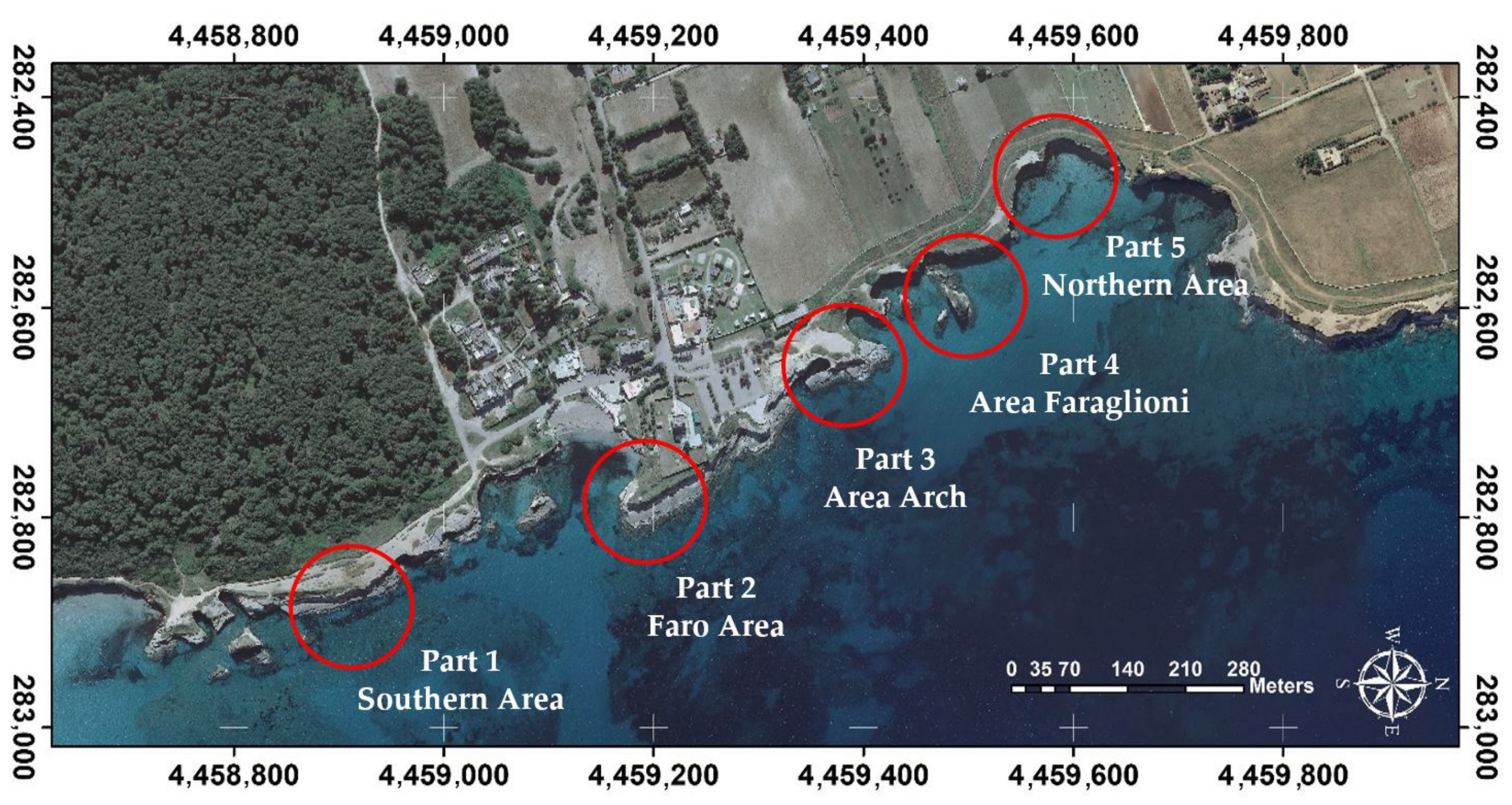
The area monitored is the coastal strip located in Sant’Andrea, in the municipality of Melendugno in the province of Lecce (southern Italy) (
Figure 2). In this area, the cliff shows repeated collapses of considerable proportions and, in particular, in the area south of the locality of S. Andrea, this phenomenon has led to a strong retreat of the coastline.
The processes of instability present in these areas, in particular geometric and geomorphologic conditions, are manifested through the collapse of individual blocks or portions of the rock mass.
The study of the stability conditions of rock cliffs (
Figure 3) is important in order to delineate the areas affected by instability, evaluate the degree of hazard, estimate the areas vulnerable at the foot and design interventions to mitigate the hazard and associated risk.
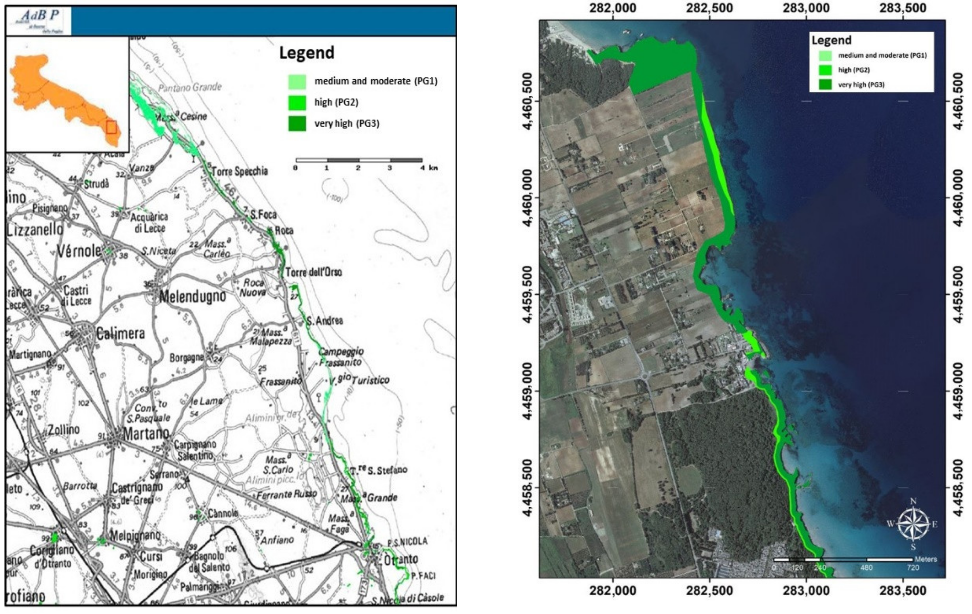
The perimeters of the geomorphological risk areas are published and constantly updated by the AdB Puglia (Apulia Basin Authority) on its official website (
www.adb.puglia.it accessed on 10 May 2021). They are subdivided into three categories of increasing risk, or rather, PG1 (medium and moderate geomorphological hazard), PG2 (high geomorphological hazard), PG3 (very high geomorphological hazard). The following figures (
Figure 4) show the classification of the area under investigation.
Melendugno municipality, the coastal stretch from Torre Specchia to Sant’Andrea, is characterized by cliffs with prevalently sub-vertical fronts, differing in height and exposure. The height of the cliffs varies from a minimum of 1 m to a maximum of about 17 m.
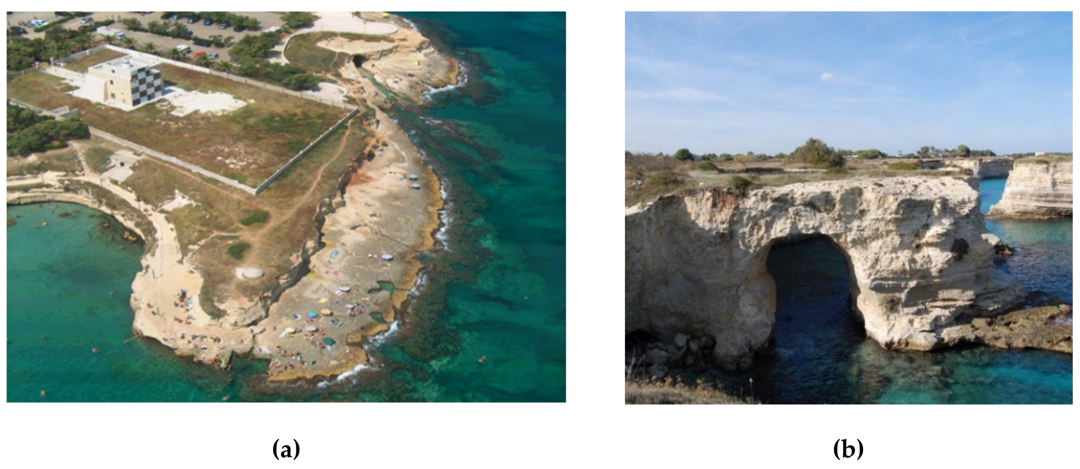
In the Sant’Andrea area, the profile of the cliffs is characterized by more complex stretches including beaches delimited by rock walls (pocket beaches). The height of the cliffs reaches a maximum of 17 m with a complex profile, which in some cases, sees the presence of a sub-horizontal platform of abrasion up to over 20 m wide (
Figure 5a,b), in others the formation of cavities and again, in some cases, at the base of the cliff, a “leaf groove” can be observed (horizontal erosive notch generally 1–1.5 m high and even a few meters deep).
In the last few years, gravitational phenomena along the cliffs of the Melendugnese coast have become more frequent. A list of the collapses that have occurred since 2013 has been drawn up on the basis of the chronicle sources found, which also show that the collapses occurred at the same time as, or following, strong sea storms and/or more or less intense precipitation. In particular, the sources record a collapse that occurred on 05 April 2013, a subsequent one involving the “Tafaluro rock” on 04 March 2018 and the last one in the upper part of the marina on 12 January 2021.
As a proof of the hazard of this area, the Otranto Maritime District Office (ordinance C.P. 22/2014) prohibited bathing in long stretches of cliffs belonging to the Municipality of Melendugno. In particular, bathing, fishing, mooring and navigation were prohibited in most of the cliff stretches classified by the Basin Plan, Hydrogeological Structure Layer (AdB Puglia, 2005, 2010) at the highest level of geomorphological hazard (PG3), in order to safeguard public safety.
3. Methodology
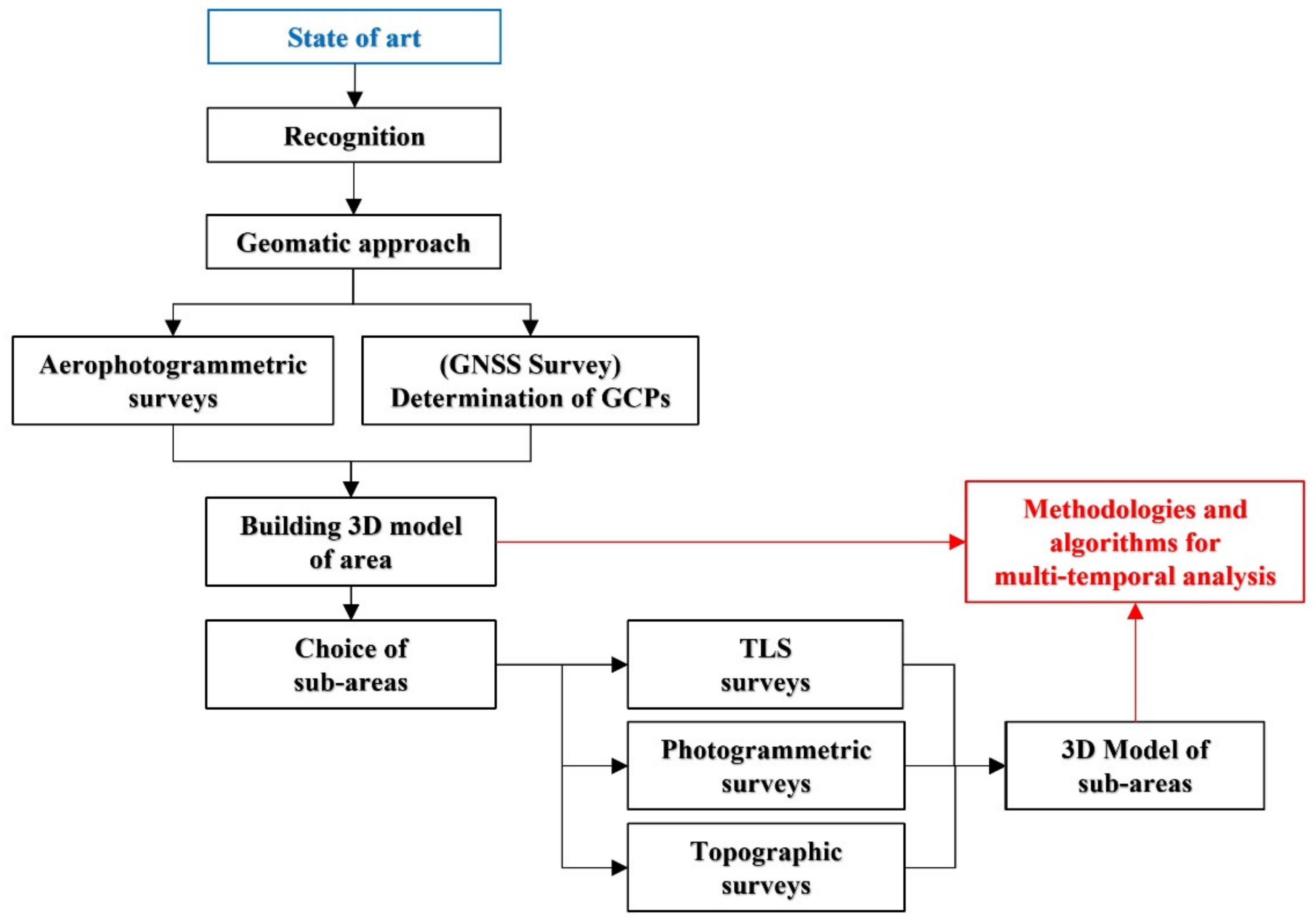
The methodology processes defined within the context of this study involved both the identification of a survey standard and the subsequent processing of the 3D models obtained with different techniques. The elaboration was carried out in a single software developed for a multi-temporal analysis of the areas to be monitored. The workflow of the adopted method can be summarised as follows (
Figure 6).
After a detailed recognition and collection of information regarding the site, the most suitable geomatics approach was selected to reconstruct the area of interest in an accurate and detailed manner. To monitor the area, a campaign of topographic (total station and Global Navigation Satellite Systems—GNSS), aerophotogrammetric, terrestrial photogrammetric and Unmanned aerial vehicle—UAV [
27,
28] and terrestrial laser scanner (TLS) surveys was carried out in order to obtain a 3D reconstruction. Repeated surveys over time enable an analysis of morphological variations and, consequently, facilitate the identification and quantification of possible instability phenomena. For the multi-temporal analysis, specific algorithms have been implemented in software.
Using integrated survey techniques, a high-resolution 3D model of the entire site was therefore created, followed by more detailed 3D models of test areas identified as being at high risk (
Figure 7).
4. Aerophotogrammetric Survey and Processing
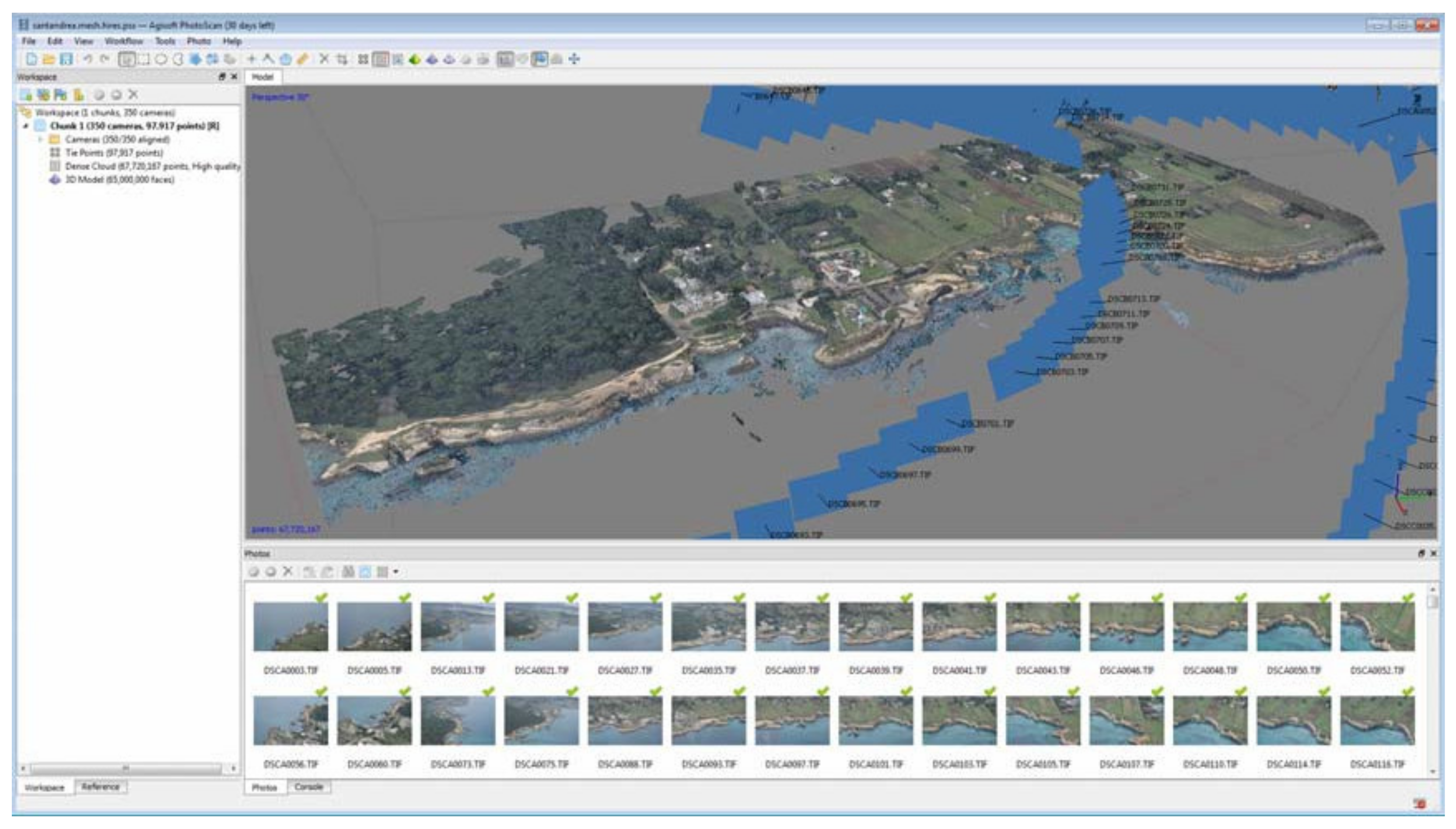
The first step was an aerophotogrammetric flight that made it possible to produce a point cloud geometric model of the area in question. In particular, a strip extending about one and a half kilometres along the coastline, at a distance of five hundred meters from the coast, was made. The requirement for an overall survey of the area was necessary for its subsequent use as a basic model for georeferencing processes alone, given the complexity of the area. In fact, on the basis of the entire 3D model, the (cartographic) overlaps of the further detailed models were implemented. The point-cloud of the aerophotogrammetric survey used as the basic model was designed and created with a spatial resolution (ground sample distance—GSD) of approximately 0.05 m. In particular, 350 photos from an aerial platform (light single-engine General Aviation aircraft) were acquired. The 3D point-cloud model of the entire area was obtained with digital photogrammetry restitution techniques with SFM (structure from motion) algorithms using Photoscan by Agisoft software. The point-cloud model was georeferenced through the identification of ground control points (GCPs) obtained with GNSS kinematic survey in post-processing with Leica GNSS GS12 geodetic receivers (dual frequency). The GNSS data processing was conducted using the permanent station of Melendugno (MELE) as a base station, belonging to the Italpos HxGN SmartNet Network (Italy). The spatial coordinates (east, north, altitude) of the 20 GCPs and the relative standard deviation (SD) values are reported in
Table 1.
The point-cloud model was generated and georeferenced in Photoscan (
Figure 8) obtaining a total error on GCPs of 0.14 m; on check points (CPs), it was of same order of magnitude. The dense clouds were subsequently exported in LAS format.
Aerophotogrammetric Point-Cloud Model into ICV Software
ICV, Intelligent Cloud Viewer, is an in-house implemented application for point cloud processing; written in C++ language with the object-oriented paradigm, compatible with Microsoft Windows 7/8/10 Operating System with 64-bit architecture [
29,
30].
ICV integrates numerous software libraries for numerical calculation, for the management of complex data structures (lists, graphs, octree, kd-tree, etc.), for computational geometry, for parallel calculation, for image processing, for computer graphics, for cartography and GIS. In particular, the software allows a number of functions, including:
management of the graphic scenery based on LOD (levels of details), which allows the real-time rendering of even very complex point clouds;
point-clouds import/export system in the most popular formats, such as LAS, LAZ, PLY, PTS, PCD, TXT, XYZ, CSV, ASC;
numerous point-cloud processing filtering techniques, such as cropping, cutting, erasing, skeletonization, transformation, colour filtering, colour transfer, simplification, outlier removal, coarse registration (match, 4-point congruent sets—4PCS and Umeyama), fine registration (iterative closest point—ICP), distance comparison (cloud-to-cloud—C2C, multiscale model-to-model cloud comparison—M3C2), volume comparison (principal component analysis—PCA), sectioning, rasterization, etc.;
reconstruction of the photogrammetric 3D model based on algorithms from the structure from motion (SfM).
In ICV, it is possible to import a LAS model, for example generated in Photoscan or 3DFZephir, using the batch-load command that permits one to translate (offset) the model during loading. The use of batch-load import is necessary whenever the point-cloud model to be imported is in cartographic projections, e.g., EPSG 32634. Through this tool, it is possible to implement a translation of the screen reference system in order to display the point cloud.
5. Terrestrial Surveys and Model Overlay Processes
After identifying the five test areas with different morphological characteristics and dissimilar problems related to the survey activities, detailed surveys were carried out. In particular, for the easily accessible areas, integrated surveys were carried out using topographic techniques for the determination of GCPs, as well as TLS and photogrammetric techniques for the 3D reconstruction of the area.
For areas that are not always accessible (e.g., due to tides, special environmental conditions) TLS surveys were conducted. For completely inaccessible areas, UAV surveys were carried out.
In particular, the TLS surveys were carried out using FARO Focus M 70 instrumentation, a time-of-flight laser distance scanner with a maximum acquisition range of 70 m, accuracy of approximately 3 mm, field of view 360° × 300° and correlated RGB information. The photogrammetric surveys were carried out using a NIKON D5000 camera and fixed 23 mm optics. The control points were surveyed using a Leica TPS 11 VIVA Total Station. Finally, the UAV photogrammetry was conducted with the DJI Mavic 2 Pro drone and Hasselblad L1D-20c camera.
In order to evaluate the monitoring process, the surveys were conducted at different times. All the elaborations were conducted in ICV software obtaining the different multi-temporal datasets of the areas. Each model was georeferenced from the global 3D model in two separate steps. In the first step, a coarse overlay (coarse registration) is performed, followed by a more precise one (fine registration). The coarse registration is carried out using the match filter that recognises the double points present in the two models and which of the two represents the reference model.
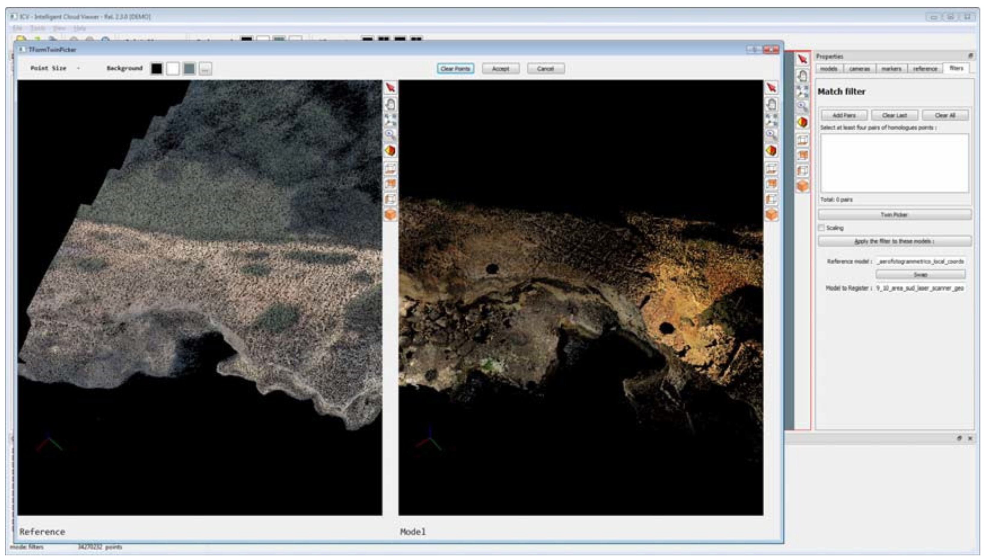
Operationally, after starting the coarse registration and identifying the reference models, a double dialogue window opens, in which the two models are displayed. For example,
Figure 9 shows the process display screen, where the global 3D model is on the left and the detail model is on the right. On both models, the four points required for the coarse registration process must be identified.
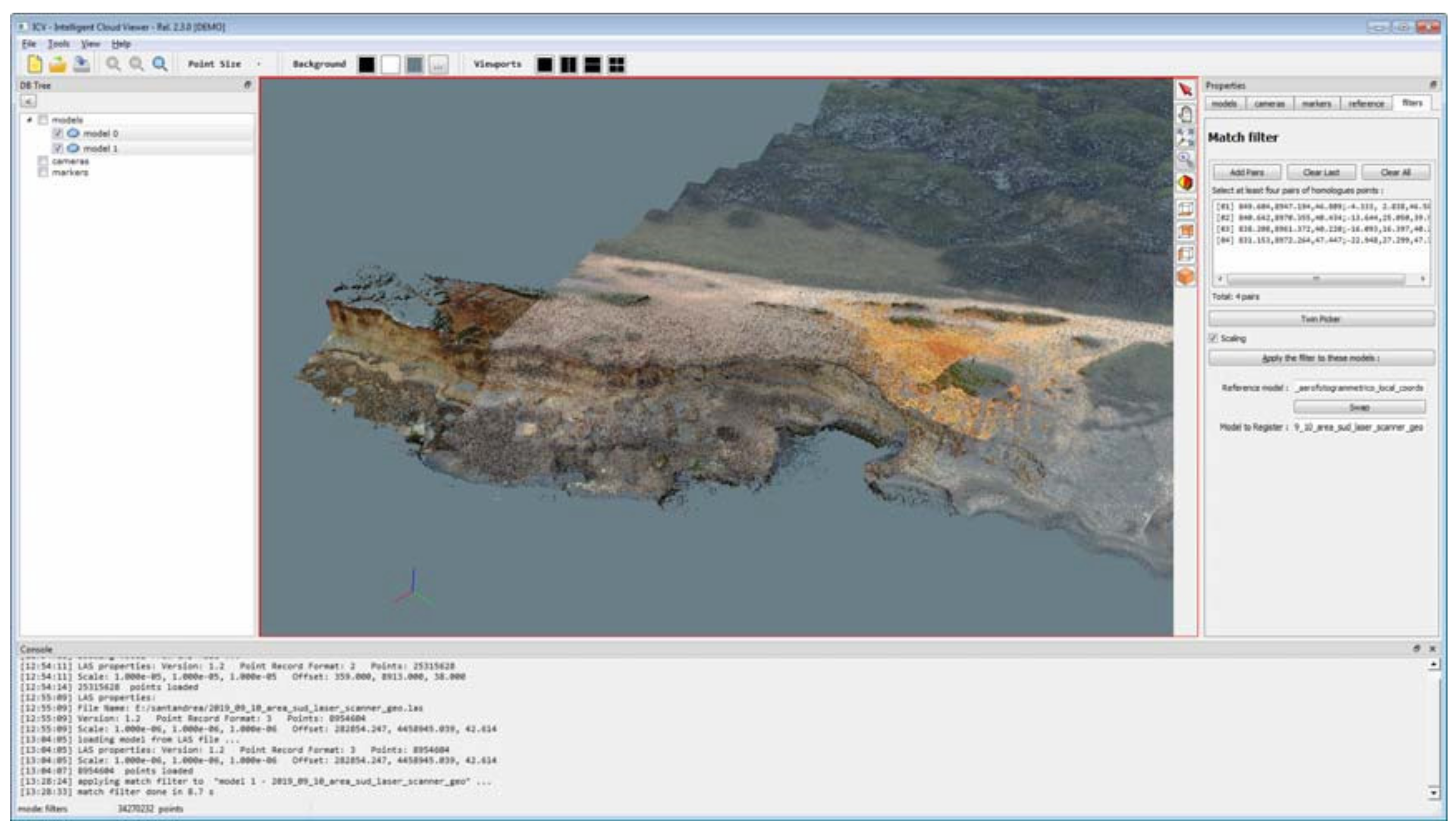
At this step, it is not necessary for the homologous points to be input with extreme precision, as the match process only guarantees the rototranslation of the models with a scale factor. The result of the process is shown in
Figure 10, where in the dialogue box to the right of the figure, the seven parameters of the transformation can be displayed.
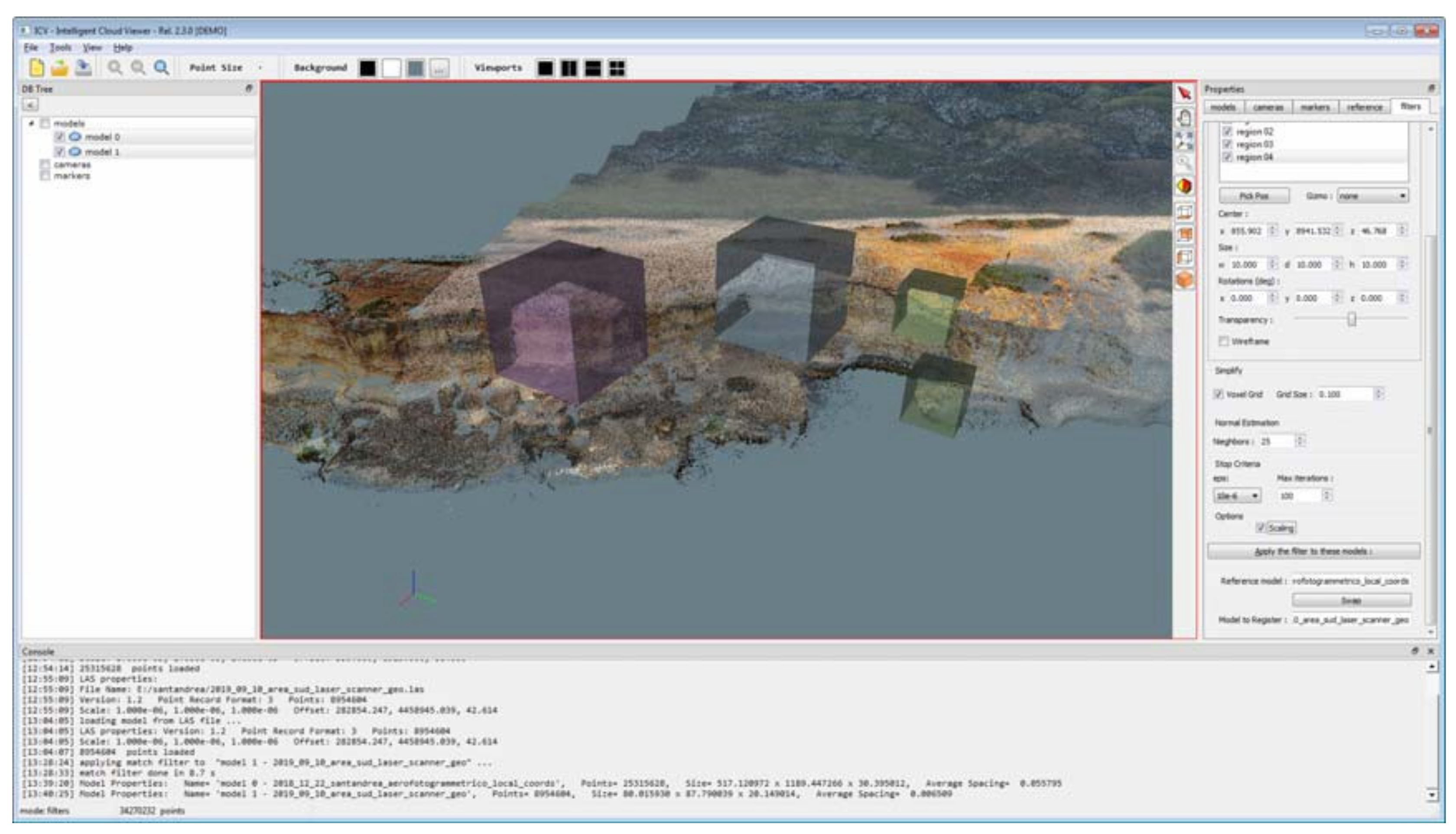
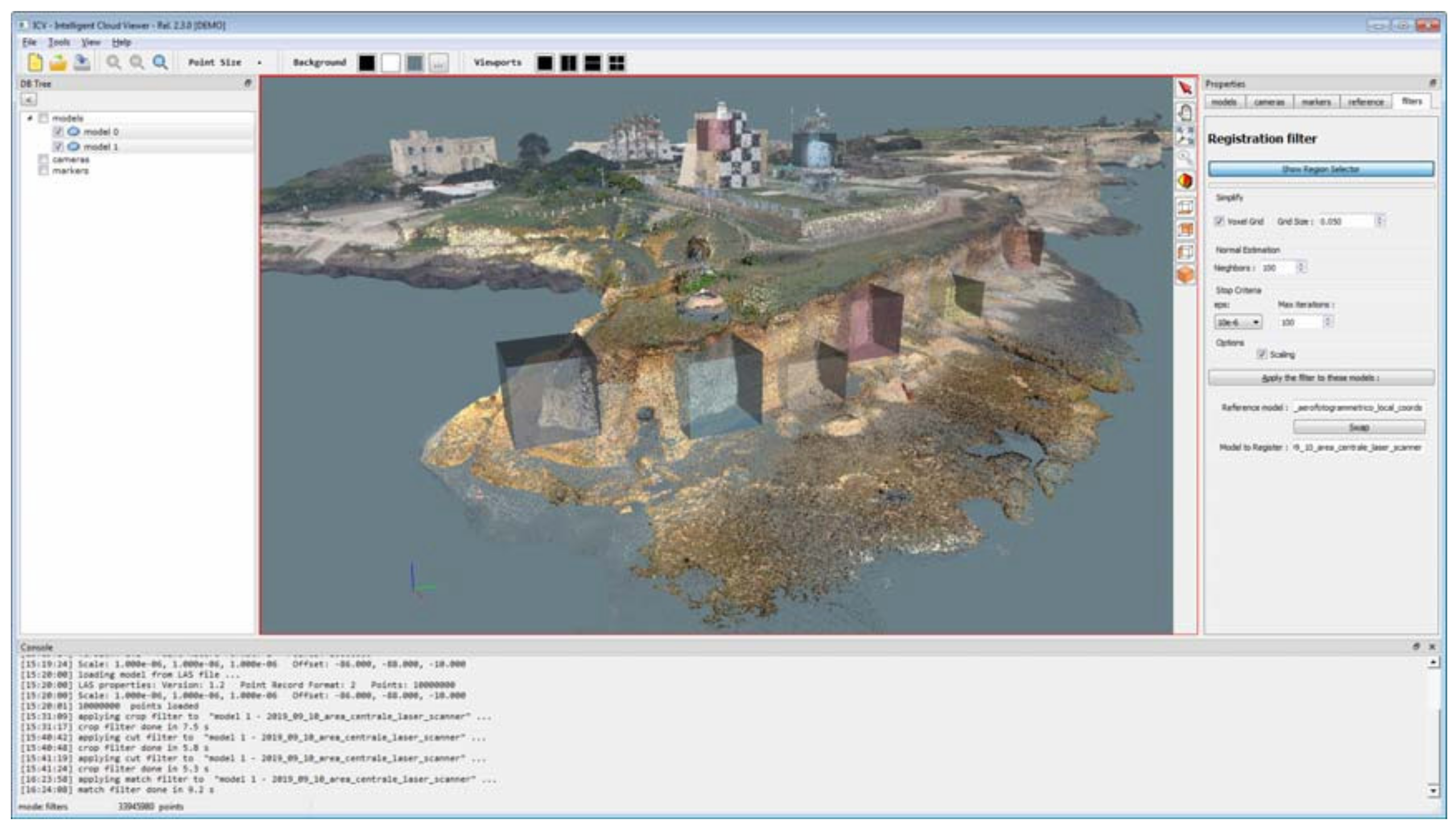
In order to speed up the fine registration process and prevent the algorithm from failing in key point matching operations, the software was designed in such a way as to limit the area of interest. This was achieved through the use of bounding boxes, i.e., a bounding box of s-points in n-dimensions. The spatial identification of bounding boxes is done manually. By generating a multiplicity of bounding boxes over significant areas (regions) (e.g., those without vegetation or with a higher percentage of overlap between models), it is possible to optimise the fine registration processes (
Figure 11).
Before performing the fine registration process, it is necessary to check the spatial resolution of the point cloud for both models, in order to further speed up the processing. This process is carried out by inserting, as input data in the voxel-grid, a value equal to or greater than the largest one relative to the resolution of the models.
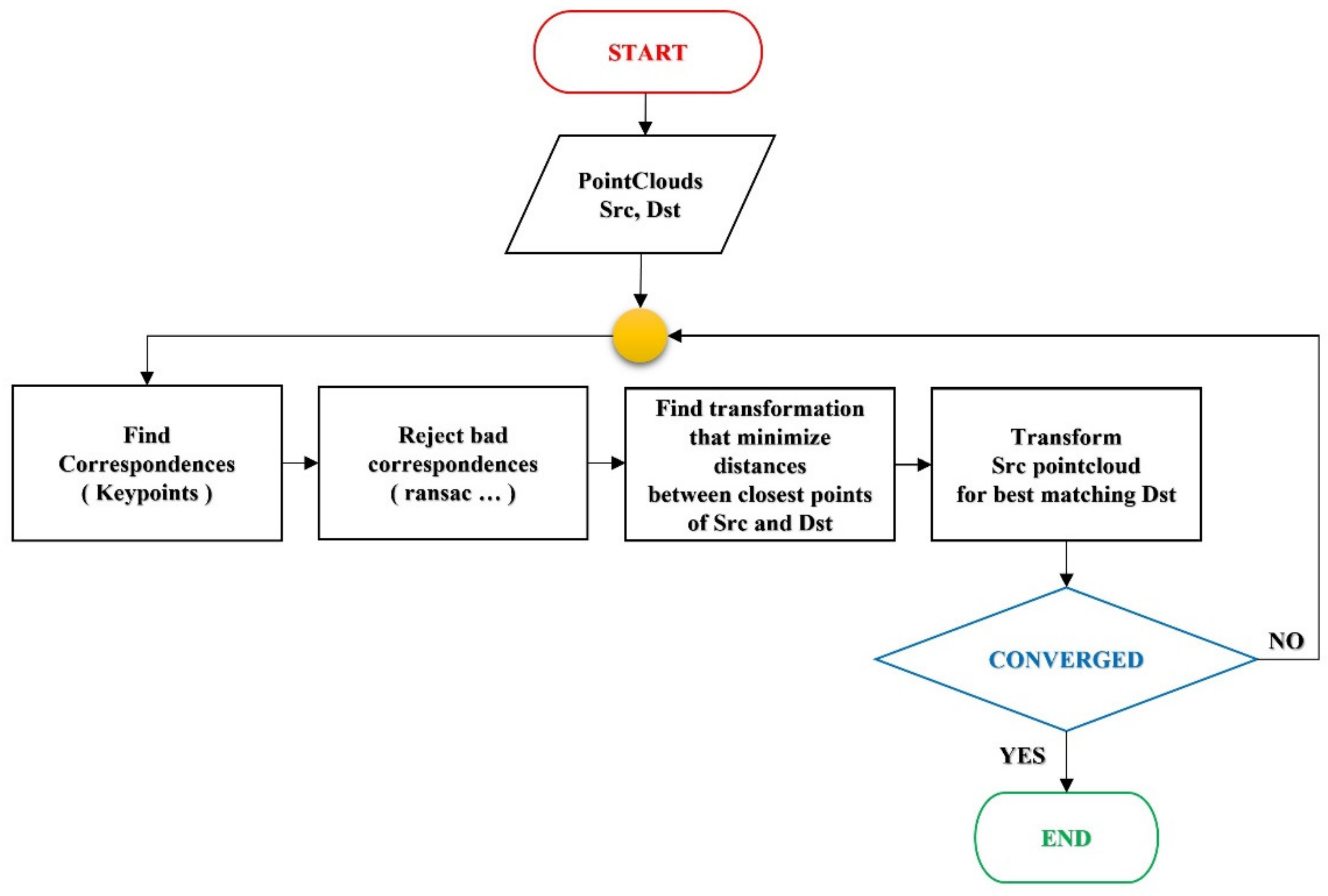
The fine registration is realized by means of an ICP algorithm implemented inside the ICV software (
Figure 12), as reported in
Appendix A (Algorithm A1). This algorithm makes it possible to minimize the distances between points belonging to two-point clouds.
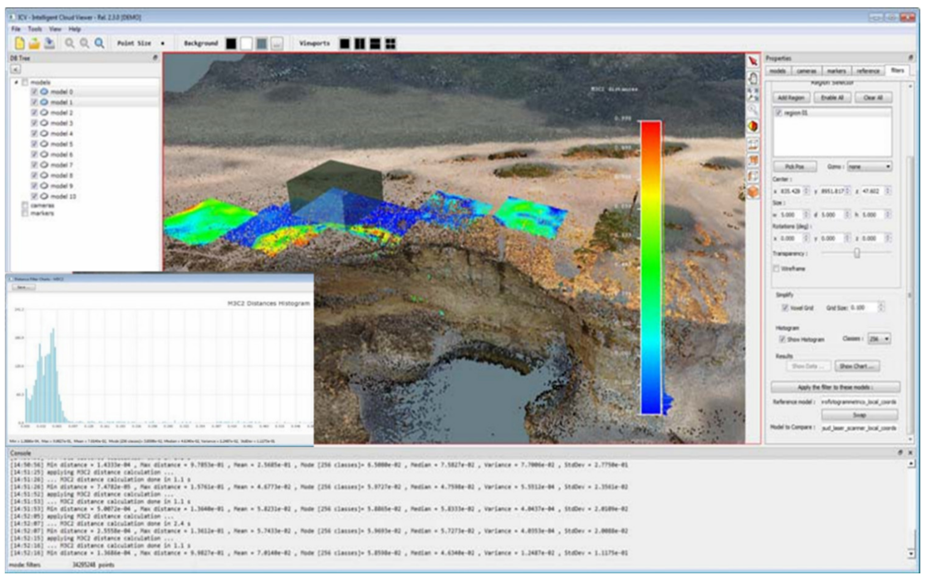
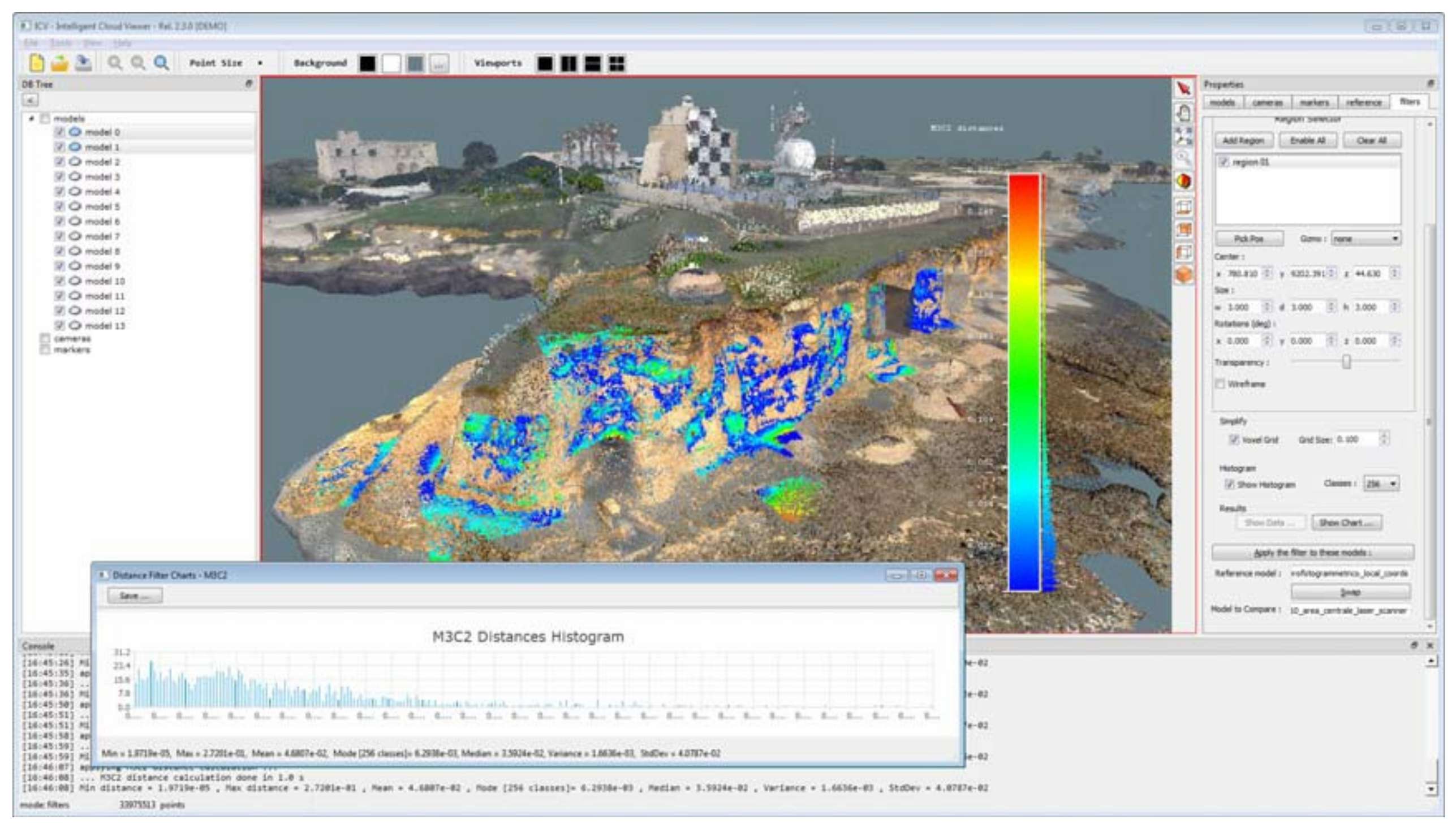
In order to evaluate the quality of the registration process, an analysis of the two datasets was performed using the distance-based filter M3C2. By selecting both models and setting up multi-bounding boxes of defined size and orientation, it is possible to check the deviations between the different point clouds. The result is visualized by means of a false-colour fingerprint on the recorded patterns, and a palette of colours is shown to highlight the distance (progressing from blue to red, the areas of least and most distance respectively), as shown in
Figure 13. In this process, distance histograms can be created.
The calculation of the difference in volumes between two-point cloud models has been implemented in ICV, using the PCA algorithm. Principal component analysis (PCA) is a method within linear transformation problems that is largely used in various fields, especially for feature extraction and dimensionality reduction.
PCA involves finding the directions of maximum variance in high-dimensional data and projecting them into a new subspace with equal or lower dimensions than the original one.
Using mathematical projection, the original data set, which may have involved many variables, is interpreted by only a few variables (called principal components).
The output of PCA is precisely these principal components, whose number is less than or equal to the number of the original variables [
31,
32].
In the case study, the PCA algorithm was used, given a cloud of points, to adapt this cloud to a Gaussian distribution in order to calculate its principal axes (plane fitting).
The centroid of such point clouds is determined by:
with
.
From this value, the covariance matrix is defined as:
with
.
The three-dimensional space (S) is uniquely defined by the mean vector, the eigenvalues of ∑, which correspond to the largest values.
The values should be normalised using the following formula:
obtaining the two eigenvectors
.
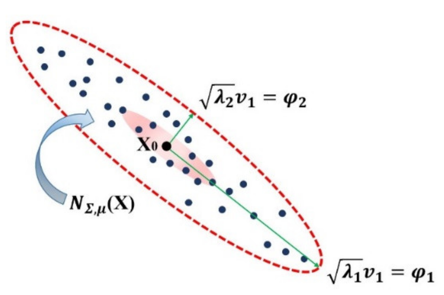
Plane fitting in 3D is calculated by firstly performing the sample mean (centroid) and then determining the two directions of maximum eigenvalues
, or the normal directions (
Figure 14).
The ratio represents the quality of the fit, or rather the optimal normal least-squares direction given by the eigenvector with small eigenvalue.
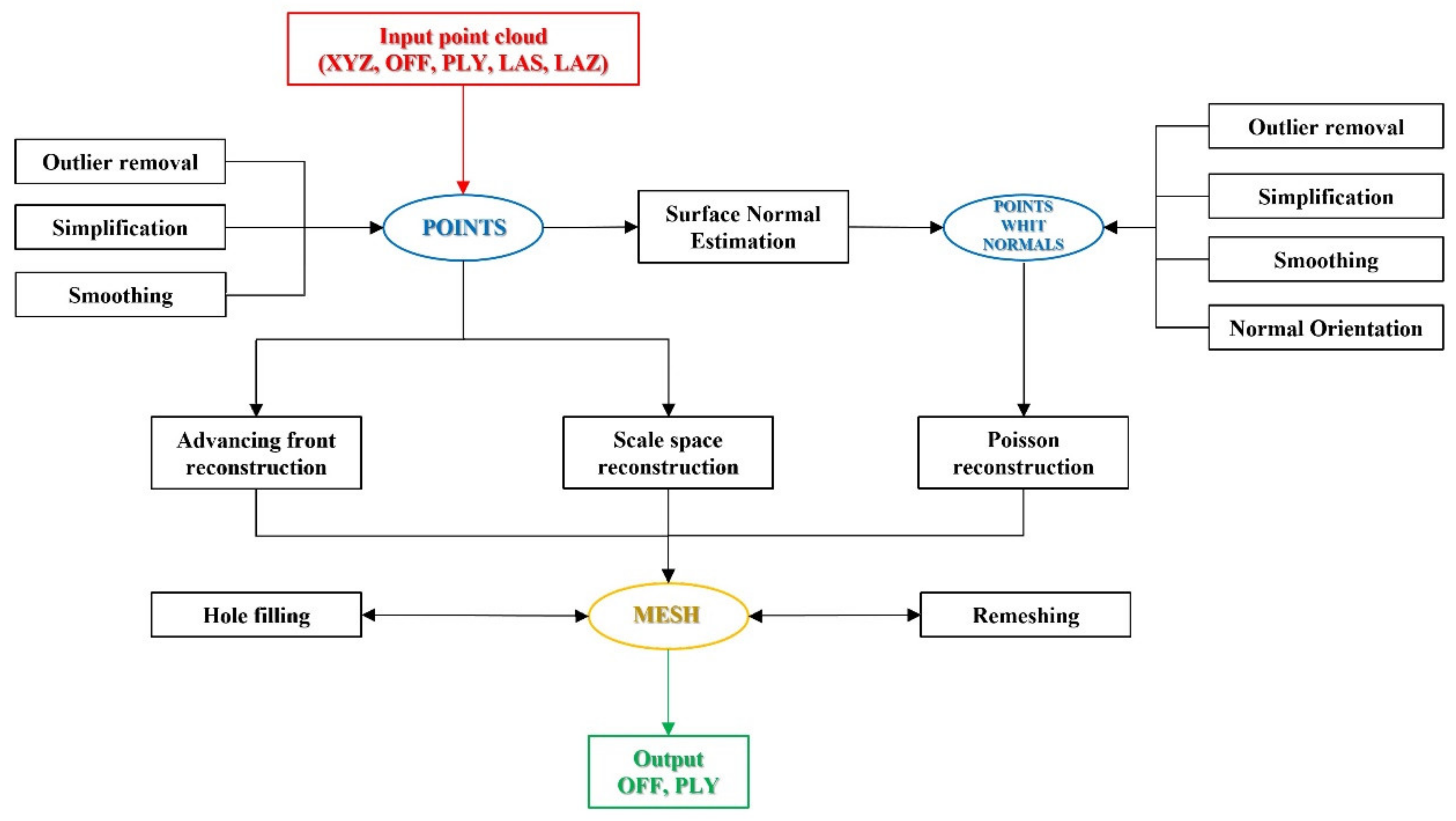
In order to calculate the difference between volumes, it is necessary to reconstruct the surfaces of the two-point clouds. Delaunay triangulation was applied to the two models. In general, the workflow leading to the calculation of the volumes can be summarized as follows (
Figure 15).
The volumetric variation, therefore, is performed by calculating the difference in volumes defined between the meshes and the fitting plane determined by PCA.
The algorithm implemented in ICV software was reported in
Appendix B (Algorithm A2).
6. Multi-Temporal Analysis on the Dataset Part 2—FARO AREA
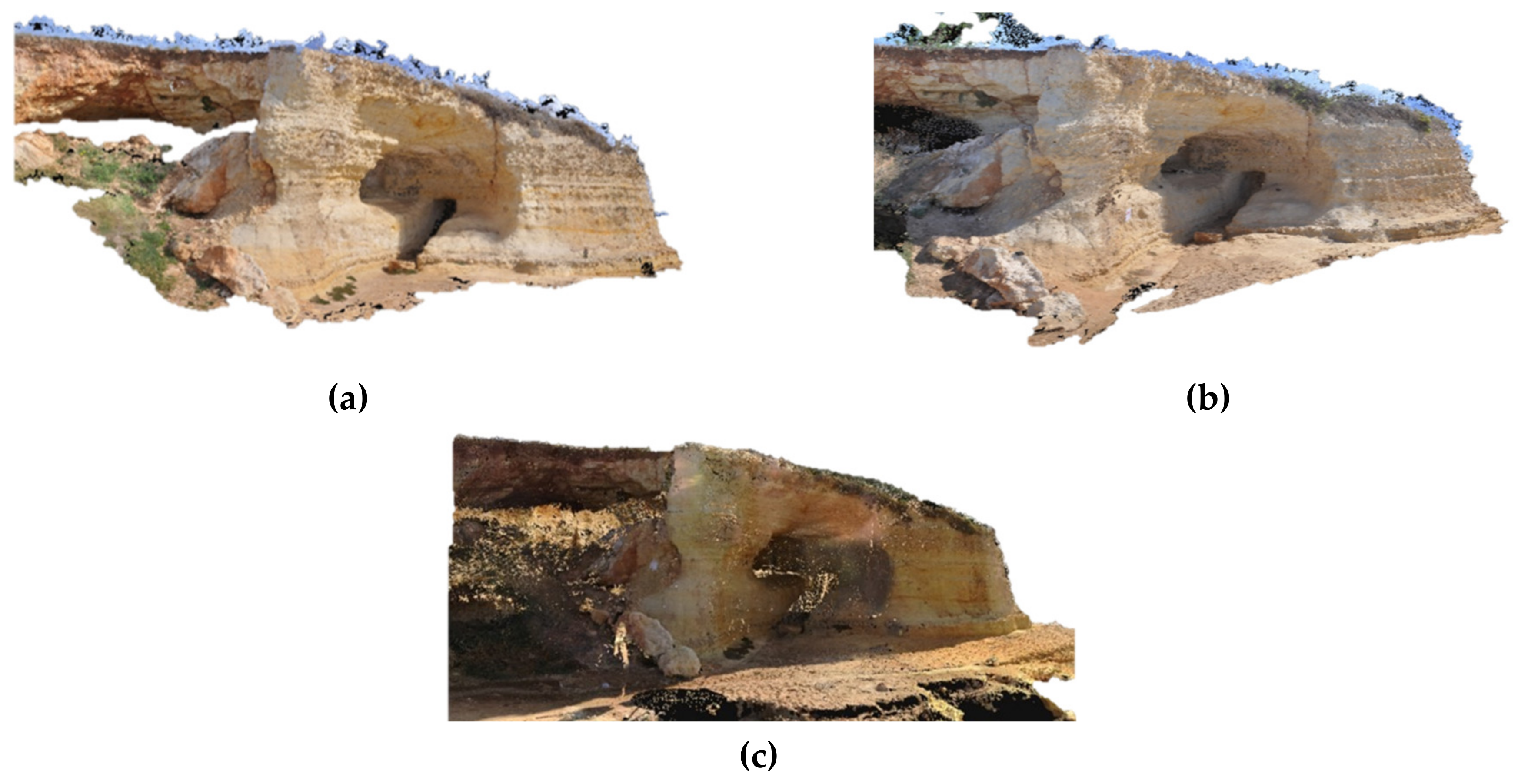
The test area shown in the manuscript is the Part 2—FARO AREA dataset. Multiple surveys have been carried out in this area. Starting from the aero-photogrammetric survey, TLS and terrestrial photogrammetric surveys were carried out at different times (
Figure 16).
Of the total georeferenced point cloud of the aerial photogrammetry, only the part belonging to the area of interest is displayed by the user (through the tool called crop). It was also possible to filter the area by eliminating data not of interest for the analysis of the rock face.
The next step was to load the data set relative to the TLS survey, which was also appropriately filtered. For the two models, the alignment processes were carried out by means of coarse registration (match filter), identifying the aerial photogrammetric model as the reference model and identifying the 4 matching points needed to start the 4PCS - Umeyama algorithm for the two clouds (
Figure 17).
For the fine registration of the models, the ICP algorithm described in
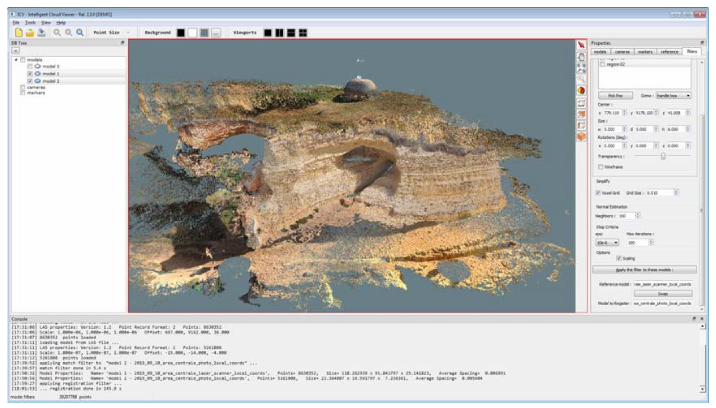
Appendix A was applied, identifying a series of bounding boxes. The choice was made by selecting areas with greater overlap, avoiding those with the presence of vegetation or other outliers, which allowed a more accurate fine registration to be obtained with lower processing speeds (
Figure 18).
The quality of the recording was verified by measuring the values of the distances between the point clouds using the M3C2 algorithm (
Figure 19).
From the TLS survey, the same procedure was used to align the terrestrial photogrammetric surveys (previously filtered) carried out at different times (
Figure 20).
The application of the M3C2 algorithm also in this case led to values for the mean and median in the order of a centimetre (mean equal to 0.018 m and standard deviation equal to 0.182 m), compatible with the limits of the instrumental acquisitions (0.07 m for the laser-scanner and 0.005 m for the photogrammetric). By carrying out the processing by means of multi bounding boxes, the results were of the sub-centimetre order in relation to the (manual) choice of including in the processing only areas, in which there were no modifications due to the presence of external elements.
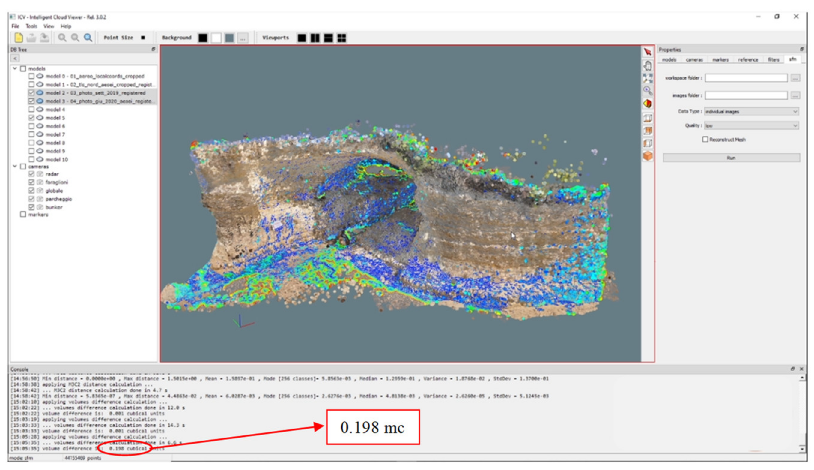
Finally, the volume difference filter was used to measure the multi-bounding boxes with morphological homogeneity over the entire rocky ridge. The volume difference recorded was only a few cubic centimetres, from which it can be deduced that the area under investigation was not affected by any appreciable geomorphological variations during the monitoring period (
Figure 21).
7. Discussion
As shown in the previous sections, different algorithms have been implemented in ICV for the multi-temporal analysis of point clouds for multiple case studies.
In particular, in the case study, the algorithms relative to the coarse registration (4PCS and Umeyama), to the fine registration (ICP), to the comparison between the post-alignment clouds (C2C, M3C2) and finally the ones relative to the calculation of the volume differences (based on the definition of the projection plane through PCA) were applied.
To validate the functionality of the ICV software, algorithms and processes implemented with open-source software were compared to the ones used.
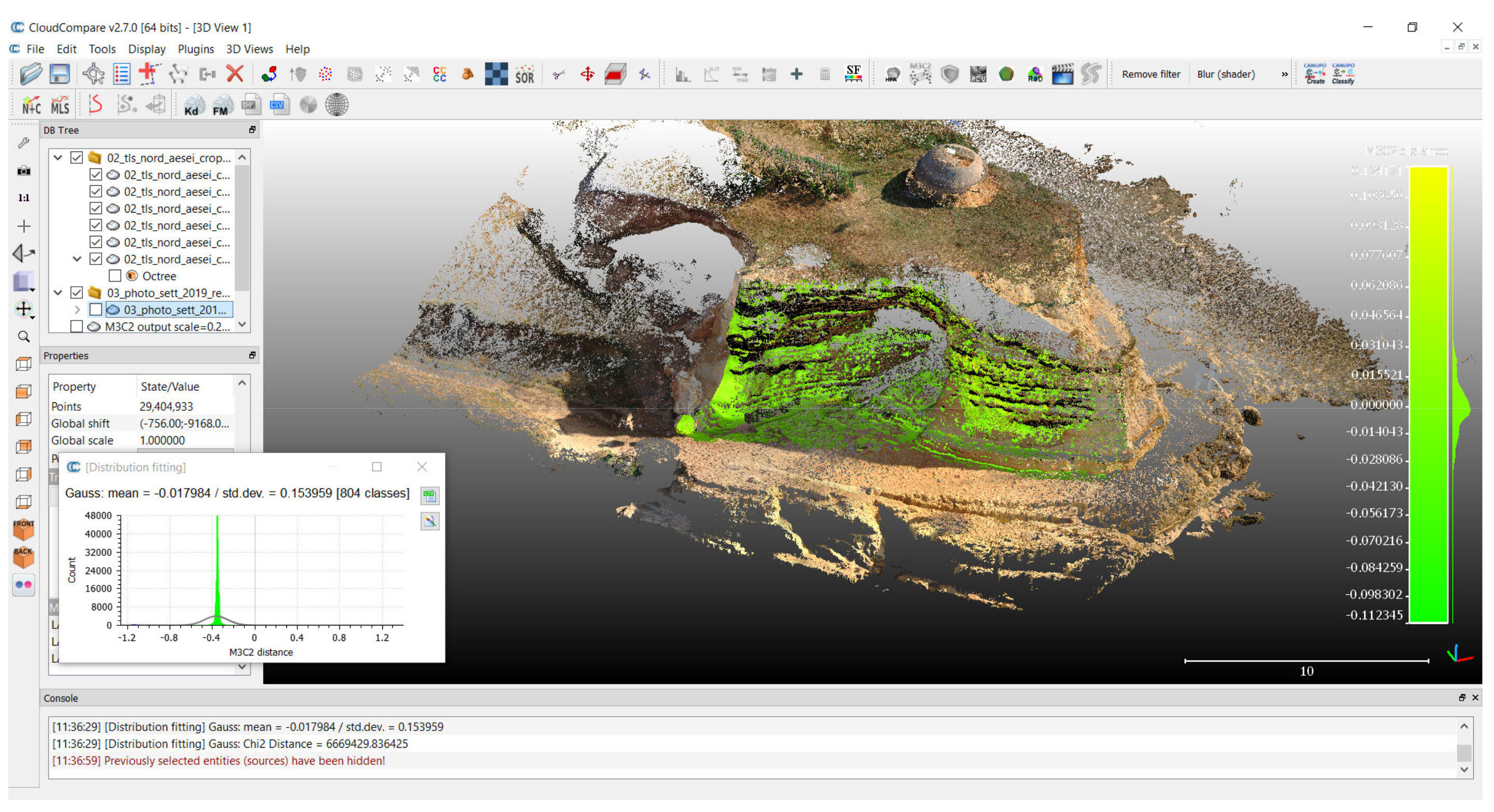
For example, the analysis of the variation of distances, using the M3C2 algorithm, was similarly conducted on Cloud Compare software (
Figure 22), obtaining values that were completely comparable to those obtained in ICV (mean of 0.018 m and standard deviation of 0.153 m).
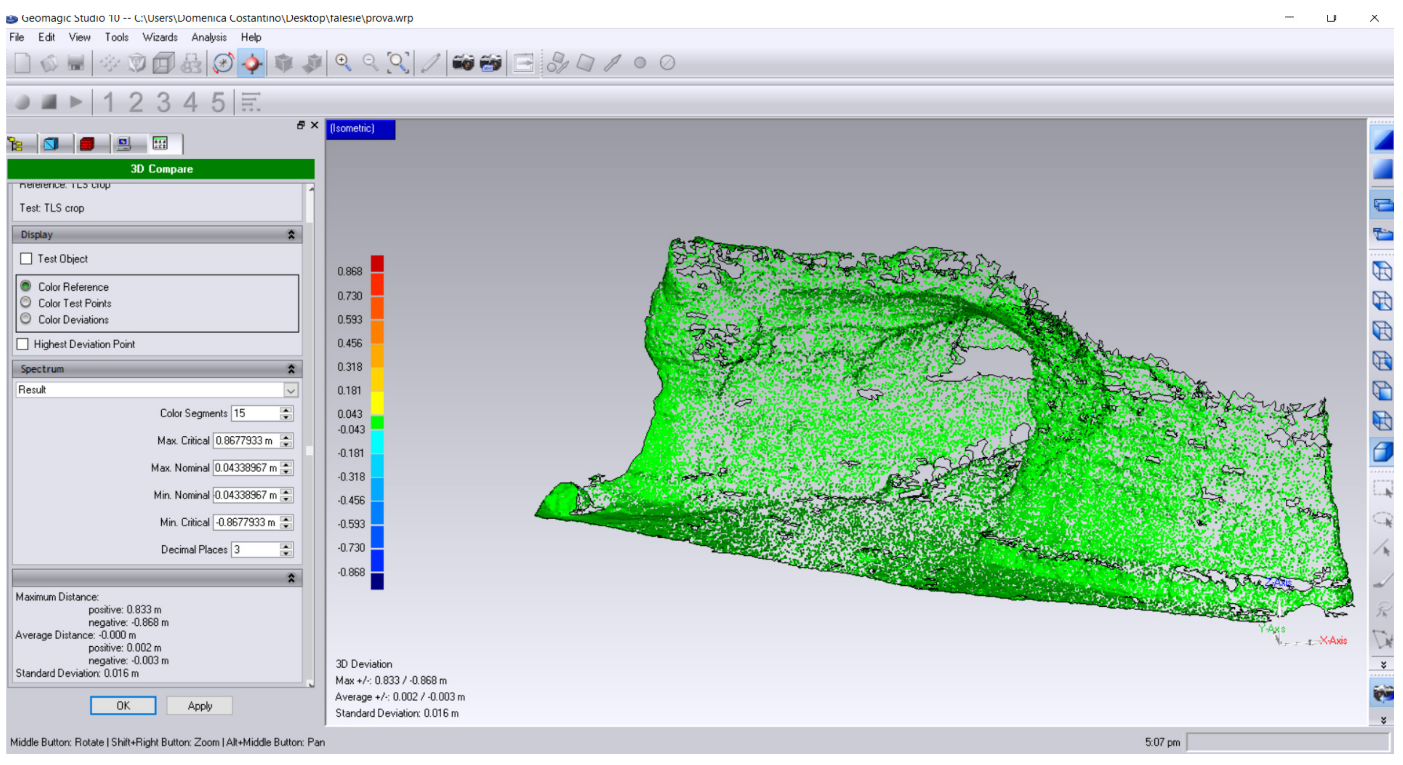
Different results were obtained in Geomagic Studio Software. In the latter software, dedicated to the processing of point clouds, the comparison of distances is performed using the 3D Compare tool. The tool, with the sampling ratio set to 100%, calculates a deviation value for each vertex in the measured data. Each measured vertex is defined by a measured position (P
m =
xm,
ym,
zm) associated with a reference position (P
r =
xr,
yr,
zr), which is defined by the projection direction (shortest, longest normal, custom). For each measured point, the tool calculates a gap vector (GV), which goes from P
r to P
m, as shown below.
This vector is converted into a scalar quantity called gap distance (D), which represents the deviation value at a given point:
As shown in
Figure 23, the values of the mean and standard deviation are 0.002 m and 0.016 m, respectively.
The algorithm implemented on ICV, relating to the determination of the difference in volumes, makes it possible to obtain an estimate of this value between the point clouds; this can be achieved either by comparing the two models or by interrogating them using the multi-bounding boxes (chosen according to the largest values recorded in M3C2).
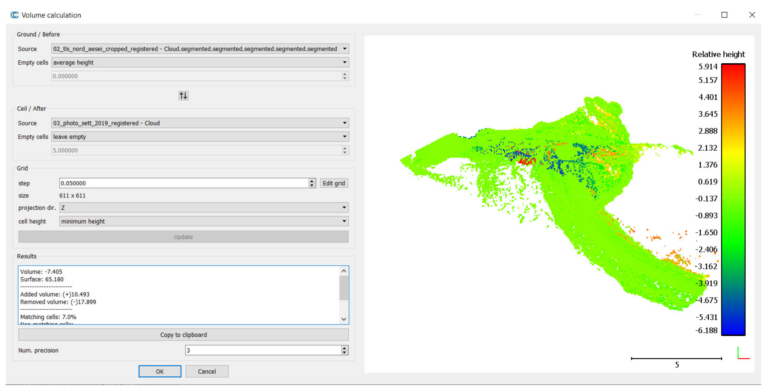
In Cloud Compare, it is possible to determine the 2.5D volumes of the point clouds; however, the calculation leading to the determination of the difference in volumes can be carried out by referring to a projection plane (X,Y—“Projection dir Z”; Y,Z—“Projection dir X”; XZ—“Projection dir Y”). Specifically, the result is the difference in volumes with respect to the chosen plane, which in our case study was approximately 7 cubic metres (
Figure 24).
The latter approach to calculating volume difference is performed similarly on Geomagic Studio software, providing the same results as Cloud Compare.
8. Conclusions
In this paper, a methodology was described for the monitoring, through geomatic techniques, of coastlines characterised by the presence of cliffs. In the case study, integrated surveys were carried out using the techniques of terrestrial photogrammetry and UAV, TLS and aerial photogrammetry for the construction of three-dimensional point cloud models.
The processing of these surveys, in order to analyse the phenomena under investigation, required the implementation of dedicated algorithms. To this end, an ad hoc software called ICV was created to manage the entire 4D monitoring process. This process was realised thanks to the implementation of algorithms for the visualisation, filtering, alignment and georeferencing, as well as the analysis of distance and volume variations.
The choice of this solution proved to be the right one, as it allowed all the processing to be carried out within a single software package. In addition, the ability to work not only on the entire point cloud, but also by means of multi-budding boxes made it possible, in the multi-time analysis, to exclude from the elaboration process any objects external to the phenomenon under investigation, such as the installation of a sealing net along a cliff wall or the presence of a different vegetation cover.
Some of the elaborations carried out on ICV were compared with those obtainable through the use of commercial software. The results of the elaborations in ICV are comparable with those of the other software examined; this confirms the quality of the algorithms implemented in the software created for the purpose.
Only one case study was presented here; however, the analysis was carried out on all 5 of the areas under investigation (
Figure 15), confirming equally reliable results obtained for the test area described in this paper.
Author Contributions
Conceptualization, D.C., F.S., M.P. and V.S.A.; methodology, D.C., F.S., M.P. and V.S.A.; software, F.S.; validation, D.C., F.S., M.P. and V.S.A.; formal analysis, D.C., F.S., M.P. and V.S.A.; investigation, D.C., F.S., M.P. and V.S.A.; resources, D.C., F.S., M.P. and V.S.A.; data curation, D.C., F.S., M.P. and V.S.A.; writing—original draft preparation, D.C., F.S., M.P. and V.S.A.; writing—review and editing, D.C., F.S., M.P. and V.S.A.; visualization, D.C., F.S., M.P. and V.S.A.; supervision, D.C., F.S., M.P. and V.S.A.; project administration, D.C.; funding acquisition, D.C. All authors have read and agreed to the published version of the manuscript.
Funding
This research was funded by Intervention co-financed within the framework of the POR Puglia FESR-FSE 2014-2020 Priority Axis 1—Research, Technological Development, Innovation - Action 1.6 “Interventi per il rafforzamento del sistema innovativo regionale e nazionale e incremento della collaborazione tra imprese e strutture di ricerca e il loro potenziamento”—Call for tenders INNONETWORK - Aid to support R&S activities. Project named COHECO Cod. 8Q2LH28 - CUP B37H17002580007.
Data Availability Statement
Data available on request due to privacy restrictions.
Acknowledgments
We want to thank the reviewers for their careful reading of the manuscript and their constructive remarks.
Conflicts of Interest
The authors declare no conflict of interest.
Appendix A
| Algorithm A1 Iterative Closest Point (ICP) Registration |
| void TICPRegistration::ICP(const PointCloud<PointT>::Ptr &src, const PointCloud<PointT>::Ptr |
| double Eps, int nMaxIter, bool bRejection, bool bScaling, Eigen::Matrix4d &transform) |
| { |
| CorrespondencesPtr all_correspondences(new Correspondences), |
| good_correspondences(new Correspondences); |
| PointCloud<PointT>::Ptr output(new PointCloud<PointT>); |
| *output = *src; |
| Eigen::Matrix4d final_transform(Eigen::Matrix4d::Identity()); |
| DefaultConvergenceCriteria<double> converged(0, transform, *good_correspondences); |
| // end cycle conditions |
| converged.setRotationThreshold(Eps); |
| converged.setTranslationThreshold(Eps); |
| converged.setMaximumIterations(nMaxIter); |
| do |
| { |
| // find correspondences (keypoints matching) |
| findCorrespondences(output, dst, *all_correspondences); |
| // reject bad correspondences (if needed) |
| // ransac + normals |
| compatibility + median distance) |
| if (bRejection) |
| { |
| rejectBadCorrespondences(all_correspondences, output, dst, |
| *good_correspondences); |
| } |
| else |
| { |
| *good_correspondences = *all_correspondences; |
| } |
| // find transformation (RT and scaling if needed) |
| findTransformation(output, dst, good_correspondences, bScaling, transform); |
| // obtain overall transformation matrix |
| final_transform = transform * final_transform; |
| // transform points |
| pcl::transformPointCloudWithNormals(*src, *output, final_transform.cast<float>()); |
| } while ( !converged.hasConverged() ); |
| transform = final_transform; |
| } |
Appendix B
| Algorithm A2 Volume difference between two point clouds |
| double TICVolumeDiferenceFilter::Apply(TPointCloud *pRefModel, TpointCloud* pModel, bool bPreprocess) |
| { |
| assert(pModel); |
| assert(pRefModel); |
| int nNeighbors = 100, nIterazions = 5; |
| double ModelAvgSpacing = cgal::TCGAL::AverageSpacing(pModel, nNeighbors); |
| double RefAvgSpacing = cgal::TCGAL::AverageSpacing(pRefModel, nNeighbors); |
| cgal::SurfaceMesh RefMesh, ModelMesh; |
| // model mesh |
| if ( bPreprocess ) |
| { |
| icv::TPCL::OutlierRemoval(pModel- >GetCloud(), pRefModel- > GetCloud(), 1.1 * |
| ModelAvgSpacing); |
| cgal::TCGAL::GridSimply(pModel, 0.5 *, ModelAvgSpacing); |
| cgal::TCGAL::JetSmoothing(pModel, nNeighbors, nIterations); |
| } |
| cgal::TCGAL::AdvancingFrontMesher (pModel, ModelMesh); |
| // reference mesh |
| if ( bPreprocess ) |
| { |
| icv::TPCL::OutlierRemoval(pRefModel- >GetCloud(), pRefModel- > GetCloud(), 1.1 * |
| RefAvgSpacing); |
| cgal::TCGAL::GridSimply(pRefModel, 0.5 *, RefAvgSpacing); |
| cgal::TCGAL::JetSmoothing(pRefModel, nNeighbors, nIterations); |
| } |
| cgal::TCGAL::AdvancingFrontMesher (pRefModel, RefMesh); |
| cgal::Kernel::Iso_cuboid_3 ModelBox = cgal::TCGAL::GetBoundingBox(pModel); |
| cgal::Kernel::Iso_cuboid_3 RefBox = cgal::TCGAL::GetBoundingBox(pRefModel); |
| double BBoxLen = std::max( cgal::TCGAL::MeanLen(ModelBox), cgal::TGAL::MeanLen(RefBox) ); |
| SbVec3d ModelCenter = cgal::TCGAL::Center(ModelBBox); |
| SbVec3d RefCenter = cgal::TCGAL::Center(RefBBox); |
| double CenterDist = SbVec3d(ModelCenter – RefCenter).length(); |
| // computes the volumes by projecting the mesh on the plane |
| // normal to ProjDir and through ProjCenter |
| // then constructs the tetrahedra and adds up their volumes |
| SbDPPlane ProjPlane; |
| cgal::TCGAL::PcaFitPlane(pRefModel, ProjPlane); |
| double IsConcordeSign = Tutils::Sign( SbVec3d(ModelCenter – |
| RefCenter).dot(ProjPlane.getNormal() ); |
| SbVec3d ProjCenter = Ref Center – Is concordSign * ProjPlane.getNormal() * BBoxLen; |
| SbDPLene Projdir(RefCenter, Projcenter); |
| SbDPMatrix xfMat = SbDPMatrix::identify(); |
| xfMat.setTraslate( -IsConcordeSign * ProjPlane.getNormal() * CenterDist ); |
| return double ( cgal::TCGAL::TetrahedraVolume(ModelMesh, ProjDir, ProjPlane) - |
| cgal::TCGAL::TetrahedraVolume(ReflMesh, ProjDir, ProjPlane)); |
References
- Pranzini, E. La forma delle coste. In Geomorfologia Costiera Impatto Antropico e Difesa dei Litorali; Zanichelli: Bologna, Italy, 2005; 245p. [Google Scholar]
- Naylor, L.A.; Stephenson, W.J.; Trenhaile, A.S. Rock coast geomorphology: Recent advances and future research directions. Geomorphology 2010, 114, 3–11. [Google Scholar]
- Sunamura, T. Processes of sea cliff and platform erosion. In CRC Handbook of Coastal Processes and Erosion; CRC Press: Boca Raton, FL, USA, 1983; pp. 233–265. [Google Scholar]
- Budetta, P.; Santo, A.; Vivenzio, F. Landslide hazard mapping along the coastline of the Cilento region (Italy) by means of a GIS-based parameter rating approach. Geomorphology 2008, 94, 340–352. [Google Scholar]
- Redweik, P.; Matildes, R.; Marques, F.M.S.F.; Santos, L. Photogrammetric methods for monitoring cliffs with low retreat rate. J. Coast. Res. 2009, 9, 1577–1581. [Google Scholar]
- Fernández, O. Obtaining a best fitting plane through 3D georeferenced data. J. Struct. Geol. 2005, 27, 855–858. [Google Scholar]
- Ruberti, D.; Marino, E.; Pignalosa, A.; Romano, P.; Vigliotti, M. Assessment of Tuff Sea Cliff Stability Integrating Geological Surveys and Remote Sensing. Case History from Ventotene Island (Southern Italy). Remote Sens. 2020, 12, 1–19. [Google Scholar]
- Kemeny, J.; Turner, K. Ground-Based LiDAR: Rock Slope Mapping and Assessment; Federal Highway Administration Report No. FHWA-CFL/TD-08-006; U.S. Department of Administration: Washington, DC, USA, 2008.
- Jaboyedoff, M.; Metzger, R.; Oppikofer, T.; Couture, R.; Derron, M.H.; Locat, J.; Turmel, D. New insight techniques to analyze rock-slope relief using DEM and 3Dimaging cloud points: COLTOP-3D software. In Proceedings of the 1st Canada-US Rock Mechanics Symposium, Vancouver, BC, Canada, 27–31 May 2007; American Rock Mechanics Association: Alexandria, VA, USA, 2007. [Google Scholar]
- Oppikofer, T.; Jaboyedoff, M.; Blikra, L.; Derron, M.H.; Metzger, R. Characterization and monitoring of the Åknes rockslide using terrestrial laser scanning. Nat. Hazards Earth Syst. Sci. 2009, 9, 1003–1019. [Google Scholar]
- Sturzenegger, M.; Stead, D. Quantifying discontinuity orientation and persistence on high mountain rock slopes and large landslides using terrestrial remote sensing techniques. Nat. Hazards Earth Syst. Sci. 2009, 9, 267–287. [Google Scholar]
- Tavani, S.; Mencos, J.; Bausà, J.; Muñoz, J.A. The fracture pattern of the Sant Corneli Bóixols oblique inversion anticline (Spanish Pyrenees). J. Struct. Geol. 2011, 33, 1662–1680. [Google Scholar]
- Slob, S.; Hack, R. 3D terrestrial laser scanning as a new field measurement and monitoring technique. In Engineering Geology for Infrastructure Planning in Europe; Springer: Berlin/Heidelberg, Germany, 2004; pp. 179–189. [Google Scholar]
- Dewez, T.J.B.; Girardeau-Montaut, D.; Allanic, C.; Rohmer, J. Facets: A cloudcompare plugin to extract geological planes from unstructured 3D point clouds. Int. Arch. Photogramm. Remote Sens. Spatial Inf. Sci. 2016, 41, B5. [Google Scholar]
- Ferrero, A.M.; Forlani, G.; Roncella, R.; Voyat, H.I. Advanced geostructural survey methods applied to rock mass characterization. Rock Mech. Rock Eng. 2009, 42, 631–665. [Google Scholar]
- Gigli, G.; Casagli, N. Semi-automatic extraction of rock mass structural data from high resolution LIDAR point clouds. Int. J. Rock Mech. Min. Sci. 2011, 48, 187–198. [Google Scholar]
- Riquelme, A.; Abellán, A.; Tomás, R.; Jaboyedoff, M. Rock slope discontinuity extraction and stability analysis from 3D point clouds: Application to an urban rock slope. In Proceedings of the Vertical Geology Conference, Lausanne, Switzerland, 6–7 February 2014. [Google Scholar]
- Riquelme, A.J.; Abellán, A.; Tomás, R. Discontinuity spacing analysis in rock masses using 3D point clouds. Eng. Geol. 2015, 195, 185–195. [Google Scholar]
- Jaboyedoff, M.; Oppikofer, T.; Abellán, A.; Derron, M.H.; Loye, A.; Metzger, R.; Pedrazzini, A. Use of LIDAR in landslide investigations: A review. Nat. Hazards 2012, 61, 5–28. [Google Scholar]
- Metzger, R.; Jaboyedoff, M.; Oppikofer, T.; Viero, A.; Galgaro, A. Coltop3D: A new software for structural analysis with high resolution 3D point clouds and DEM. AAPG Search Discov. Artic. 2009, 90171, 4–8. [Google Scholar]
- Castiglioni, G.B. Geomorfologia; Unione Tipografico-Editrice Torinese: Torino, Italy, 1979. [Google Scholar]
- Sunamura, T. Geomorphology of Rocky Coasts; John Wiley & Son Ltd: Chichester, UK, 1992; Volume 3. [Google Scholar]
- Simeoni, U.; Corbau, C.; Pranzini, E.; Ginesu, S. Le pocket beach. In Dinamica e Gestione Delle Piccole Spiagge; FrancoAngelli: Milan, Italy, 2012. [Google Scholar]
- Javadnejad, F.; Slocum, R.K.; Gillins, D.T.; Olsen, M.J.; Parrish, C.E. Dense Point cloud quality factor as proxy for accuracy assessment of image-based 3D reconstruction. J. Surv. Eng. 2021, 147, 04020021. [Google Scholar]
- Abellan, A.; Derron, M.H.; Jaboyedoff, M. Use of 3D Point Clouds in Geohazards. Remote Sens. 2016, 8, 130. [Google Scholar]
- Lollino, P.; Pagliarulo, R.; Trizzino, R.; Santaloia, F.; Pisano, L.; Zumpano, V.; Perrotti, M.; Fazio, N.L. Multi-scale approach to analyse the evolution of soft rock coastal cliffs and role of controlling factors: A case study in South-Eastern Italy. Geomat. Nat. Hazards Risk 2021, 12, 1058–1081. [Google Scholar]
- Alfio, V.S.; Costantino, D.; Pepe, M. Influence of Image TIFF Format and JPEG Compression Level in the Accuracy of the 3D Model and Quality of the Orthophoto in UAV Photogrammetry. J. Imaging 2020, 6, 30. [Google Scholar]
- Pepe, M.; Costantino, D. UAV Photogrammetry and 3D Modelling of Complex Architecture for Maintenance Purposes: The Case Study of the Masonry Bridge on the Sele River, Italy. Period. Polytech. Civ. Eng. 2021, 65, 191–203. [Google Scholar]
- Costantino, D.; Angelini, M.G.; Settembrini, F. ICV and fine-registration algorithms for an efficient merging of point clouds. In Proceedings of the IMEKO International Conference on Metrology for Archaeology and Cultural Heritage (MetroArchaeo), Lecce, Italy, 23–25 October 2017. [Google Scholar]
- Costantino, D.; Angelini, M.G.; Settembrini, F. Point cloud management through the realization of the Intelligent Cloud Viewer software. Int. Arch. Photogramm. Remote Sens. Spat. Inf. Sci. 2017, 42, 105–112. [Google Scholar]
- Chen, Y.; Medioni, G. Object modelling by registration of multiple range images. Image Vis. Comput. 1992, 10, 145–155. [Google Scholar]
- Alakkari, S.; Dingliana, J. Volume visualization using principal component analysis. In Proceedings of the Eurographics Workshop on Visual Computing for Biology and Medicine, Bergen, Norway, 7–9 September 2016; pp. 53–57. [Google Scholar]
Figure 1.
Classification of cliffs (modified from Sunamura, 1983; 1992).
Figure 1.
Classification of cliffs (modified from Sunamura, 1983; 1992).
Figure 2.
Study area: (a) identification of the area of interest and (b) orthophoto.
Figure 2.
Study area: (a) identification of the area of interest and (b) orthophoto.
Figure 3.
Overview of the Sant’Andrea coastline.
Figure 3.
Overview of the Sant’Andrea coastline.
Figure 4.
Thematic maps of geomorphological hazard zones.
Figure 4.
Thematic maps of geomorphological hazard zones.
Figure 5.
Cliffs with: (a) presence of a sub-horizontal platform and (b) cavity formations and leaf groove.
Figure 5.
Cliffs with: (a) presence of a sub-horizontal platform and (b) cavity formations and leaf groove.
Figure 6.
Workflow of implemented method.
Figure 6.
Workflow of implemented method.
Figure 7.
Identification of the five detailed areas.
Figure 7.
Identification of the five detailed areas.
Figure 8.
Print screen of the processes performed in Photoscan software.
Figure 8.
Print screen of the processes performed in Photoscan software.
Figure 9.
Visualization of the course registration process.
Figure 9.
Visualization of the course registration process.
Figure 10.
Result of course registration process.
Figure 10.
Result of course registration process.
Figure 11.
Detection of bounding boxes on models.
Figure 11.
Detection of bounding boxes on models.
Figure 12.
Workflow of the algorithm in ICV for the end registration.
Figure 12.
Workflow of the algorithm in ICV for the end registration.
Figure 13.
Result of point cloud comparison in fine registration.
Figure 13.
Result of point cloud comparison in fine registration.
Figure 14.
Graphical representation of the two directions of maximum eigenvalues.
Figure 14.
Graphical representation of the two directions of maximum eigenvalues.
Figure 15.
Surface calculation workflow.
Figure 15.
Surface calculation workflow.
Figure 16.
Surveys performed: (a) terrestrial photogrammetric survey of 16 March 2019; (b) terrestrial photogrammetric survey of 14 September 2019 and 16 June 2020; (c) TLS survey of 20 July 2019.
Figure 16.
Surveys performed: (a) terrestrial photogrammetric survey of 16 March 2019; (b) terrestrial photogrammetric survey of 14 September 2019 and 16 June 2020; (c) TLS survey of 20 July 2019.
Figure 17.
Course registration phase between aero-photogrammetric and TLS: (a) window for identifying duplicate points, (b) result of the process.
Figure 17.
Course registration phase between aero-photogrammetric and TLS: (a) window for identifying duplicate points, (b) result of the process.
Figure 18.
Choice of bounding boxes for end of registration.
Figure 18.
Choice of bounding boxes for end of registration.
Figure 19.
Results of M3C2 application.
Figure 19.
Results of M3C2 application.
Figure 20.
Result of fine registration between TLS and terrestrial photogrammetry.
Figure 20.
Result of fine registration between TLS and terrestrial photogrammetry.
Figure 21.
Calculation of volume difference in ICV software.
Figure 21.
Calculation of volume difference in ICV software.
Figure 22.
Analysis of the variation of distances, using the M3C2 algorithm, in Cloud Compare.
Figure 22.
Analysis of the variation of distances, using the M3C2 algorithm, in Cloud Compare.
Figure 23.
Analysis of the variation of distances in Geomagic software.
Figure 23.
Analysis of the variation of distances in Geomagic software.
Figure 24.
Calculation of the 2D volumes in Cloud Compare.
Figure 24.
Calculation of the 2D volumes in Cloud Compare.
Table 1.
Points coordinates in UTM34N-ETRF2000 and SD values (values in metres).
Table 1.
Points coordinates in UTM34N-ETRF2000 and SD values (values in metres).
| Point ID | Easting | Northing | Ellip. Hgt | SD E | SD N | SD H |
|---|
| 1 | 282,835.990 | 4,458,952.874 | 45.764 | 0.001 | 0.005 | 0.007 |
| 3 | 282,792.233 | 4,459,026.287 | 44.659 | 0.002 | 0.000 | 0.003 |
| 4 | 282,726.491 | 4,459,020.339 | 46.603 | 0.005 | 0.011 | 0.013 |
| 6 | 282,669.651 | 4,459,127.697 | 40.691 | 0.005 | 0.009 | 0.007 |
| 7 | 282,671.707 | 4,459,164.184 | 42.416 | 0.013 | 0.016 | 0.067 |
| 8 | 282,784.631 | 4,459,189.625 | 44.657 | 0.002 | 0.012 | 0.007 |
| 9 | 282,641.879 | 4,459,251.223 | 46.639 | 0.014 | 0.003 | 0.034 |
| 10 | 282,696.758 | 4,459,263.089 | 46.358 | 0.002 | 0.013 | 0.009 |
| 11 | 282,684.040 | 4,459,293.842 | 46.038 | 0.011 | 0.001 | 0.035 |
| 12 | 282,637.049 | 4,459,391.372 | 45.613 | 0.004 | 0.000 | 0.011 |
| 13 | 282,531.283 | 4,459,361.864 | 48.499 | 0.015 | 0.016 | 0.034 |
| 14 | 282,562.329 | 4,459,435.317 | 46.946 | 0.014 | 0.019 | 0.038 |
| 15 | 282,509.532 | 4,459,533.229 | 47.723 | 0.013 | 0.018 | 0.042 |
| 16 | 282,400.509 | 4,459,498.265 | 49.883 | 0.017 | 0.020 | 0.049 |
| 17 | 282,465.162 | 4,459,678.228 | 47.285 | 0.019 | 0.014 | 0.039 |
| 18 | 282,554.578 | 4,459,749.689 | 46.300 | 0.012 | 0.016 | 0.001 |
| 19 | 282,621.708 | 4,459,853.693 | 45.767 | 0.008 | 0.002 | 0.002 |
| 20 | 282,567.667 | 4,459,961.576 | 47.740 | 0.012 | 0.053 | 0.064 |
| Publisher’s Note: MDPI stays neutral with regard to jurisdictional claims in published maps and institutional affiliations. |
© 2021 by the authors. Licensee MDPI, Basel, Switzerland. This article is an open access article distributed under the terms and conditions of the Creative Commons Attribution (CC BY) license (https://creativecommons.org/licenses/by/4.0/).


 ,
, 


