
Estimation of Long-Term Surface Downward Longwave Radiation over the Global Land from 2000 to 2018

 ,
,  ,
,  and
and
Abstract

1. Introduction
2. Data
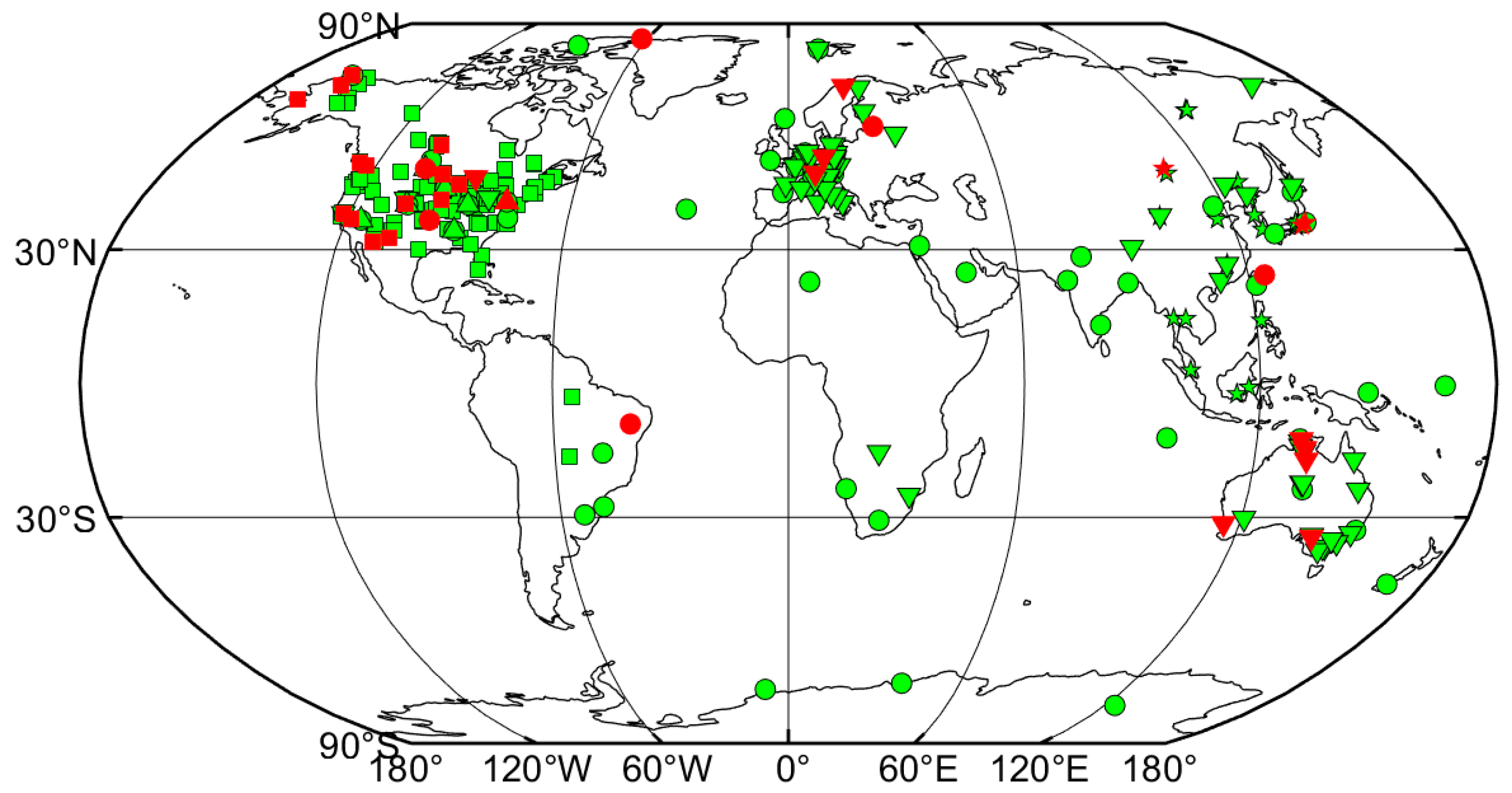
2.1. Ground Measurements
2.1.1. AmeriFlux, AsiaFlux, and FLUXNET Data
2.1.2. BSRN Data
2.1.3. SURFRAD Data
2.2. Input Data
2.2.1. ERA5 Reanalysis Dataset
2.2.2. GLASS Surface Downward Shortwave Radiation Product
2.2.3. Global Multi-Resolution Terrain Elevation Data 2010
2.3. Exiting Surface Downward Longwave Radiation Datasets
3. Method
3.1. Gradient Boosting Regression Tree
3.2. Model Construction
- (1)
- Calculating daily Ld observations. The daily mean Ld was integrated from the instantaneous values if the missing instantaneous values were less than 20% in one day because the AmeriFlux, AsiaFlux, BSRN, and SURFRAD networks only provide instantaneous Ld values;
- (2)
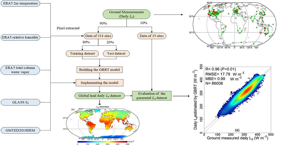
- Data preprocessing. After resampling to a 5-km resolution, the ERA5 Ta, ERA5 RH, ERA5 TCWV, GLASS Sd, and GMTED2010DEM elevation datasets were extracted according to the latitude, longitude, and time corresponding to the ground stations;
- (3)
- Training the GBRT model. By circulating within the range of each parameter displayed in Table 1, the GBRT model where the n-estimator parameter is set to 50, the learning rate is set to 0.1, the max-depth is set to 6, and the subsample parameter of 0.8 was selected as the optimal model to estimate global land Ld, achieving the lowest RMSE and MBE values on the test dataset;
- (4)
- Implementing the model. The global land Ld was produced on the basis of the trained model using the daily ERA5 Ta, ERA5 RH, ERA5 TCWV, GLASS Sd, and GMTED2010DEM elevation datasets;
- (5)
- Evaluation of the generated global land Ld dataset. Daily Ld values collected at 35 observation sites were used to validate the generated global land Ld dataset and compare it with the existing Ld datasets. The main flowchart in this study is shown in Figure 2.
4. Results
4.1. Validation against Ground Measurements
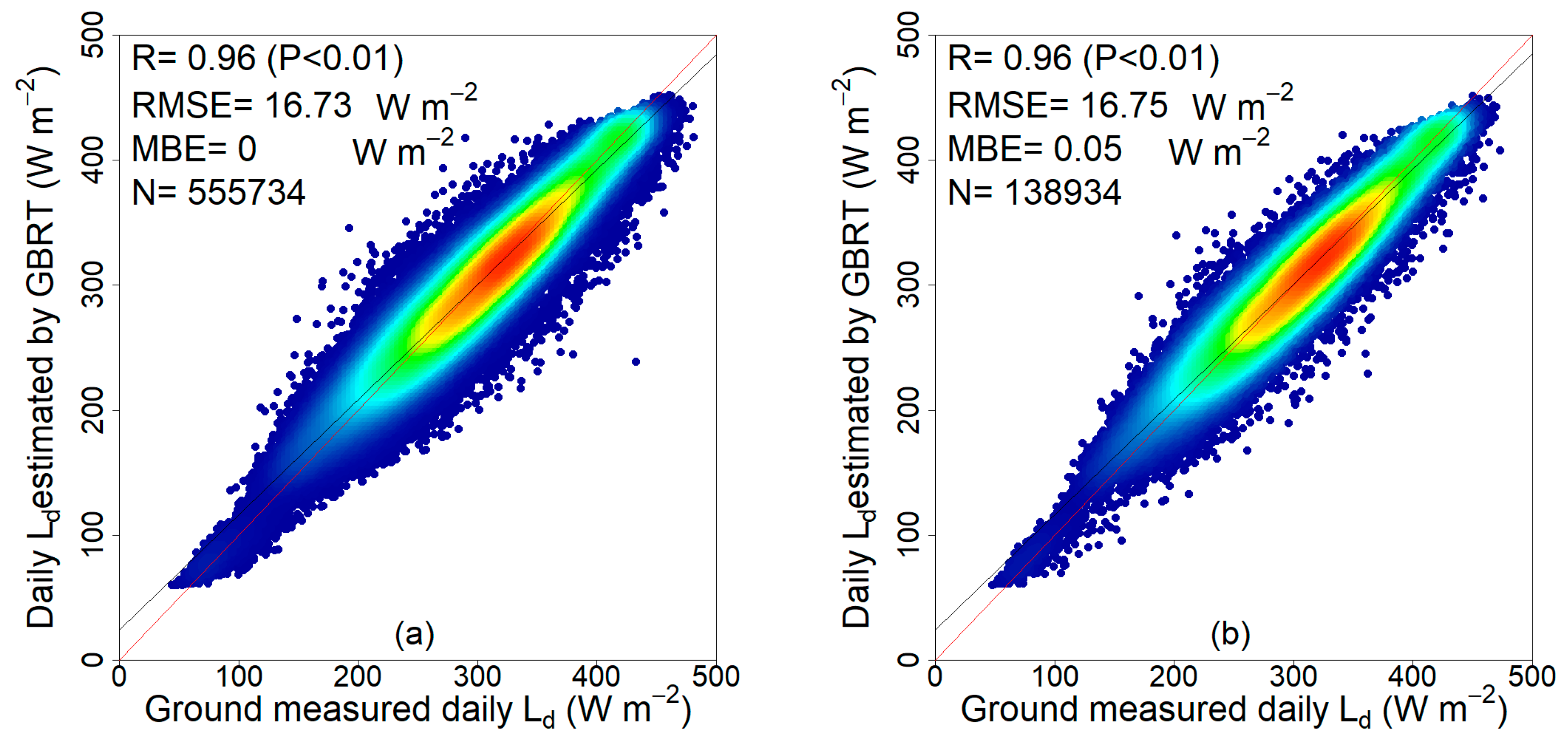
4.1.1. Performance of the Model
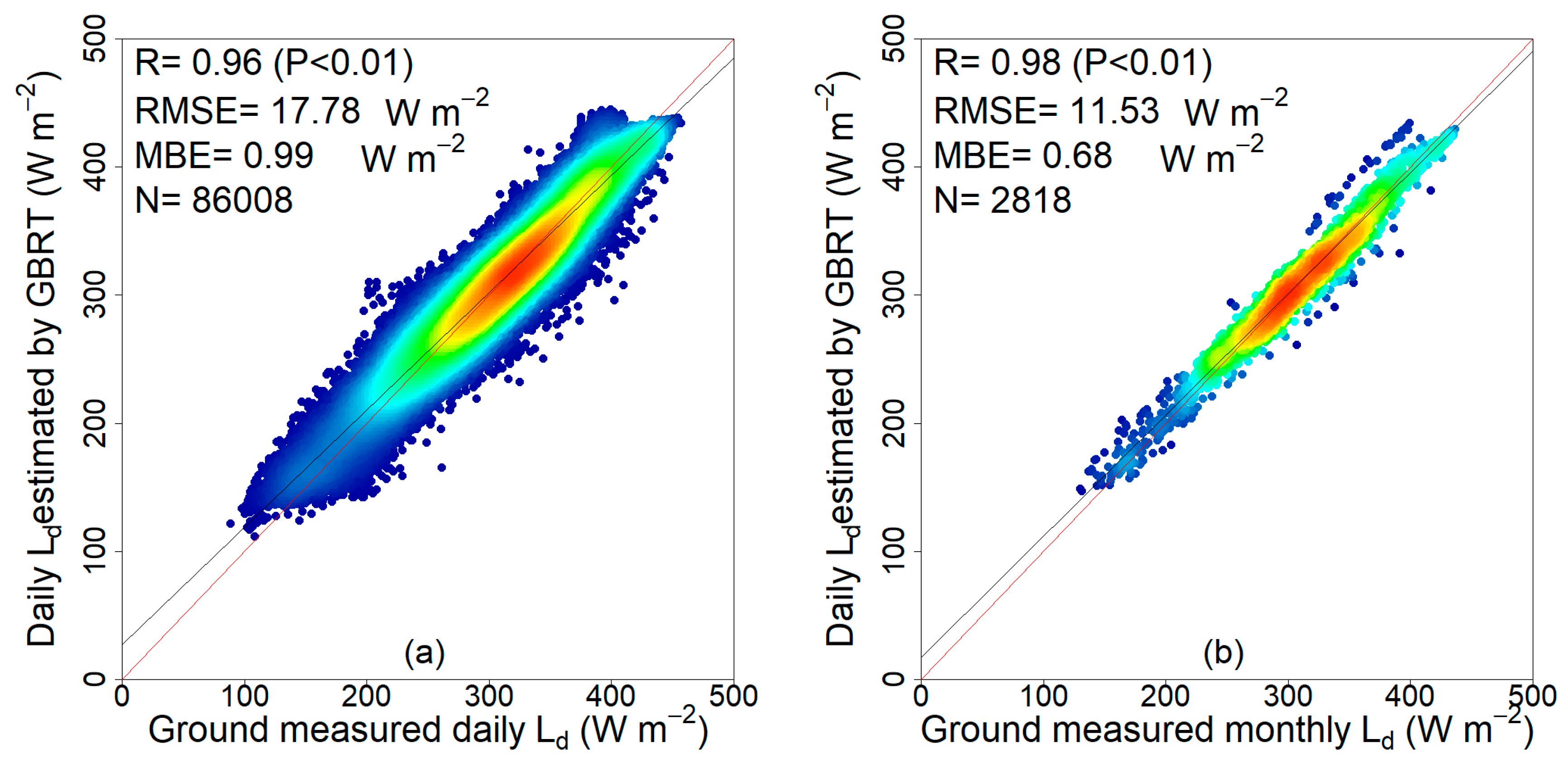
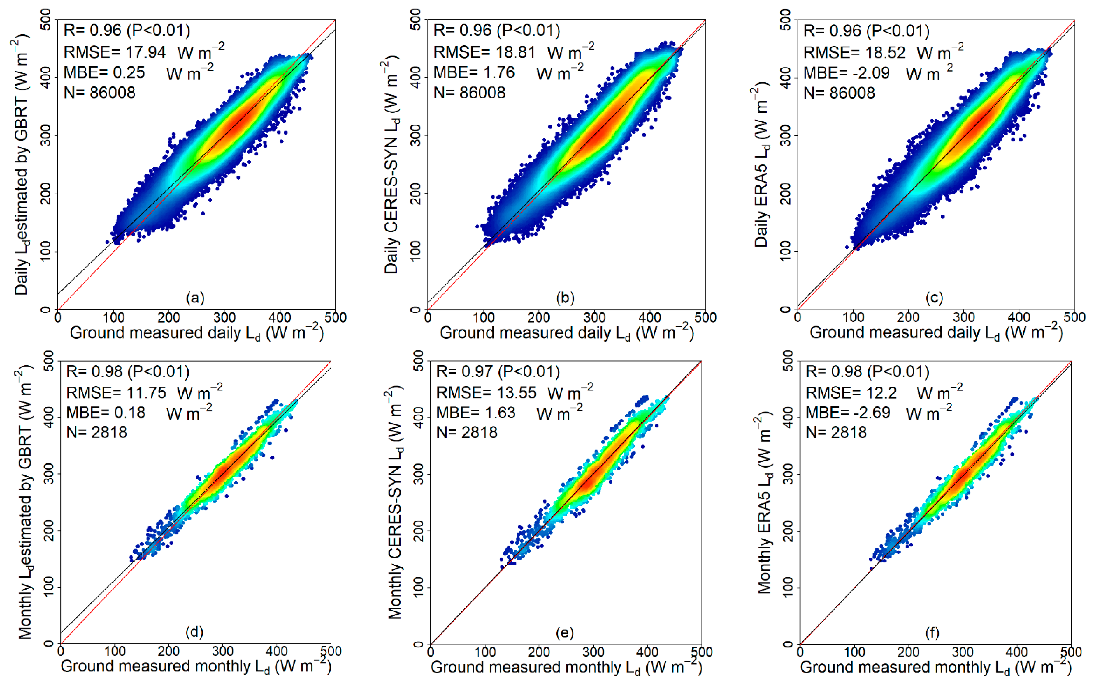
4.1.2. Validation of the Generated Ld Dataset
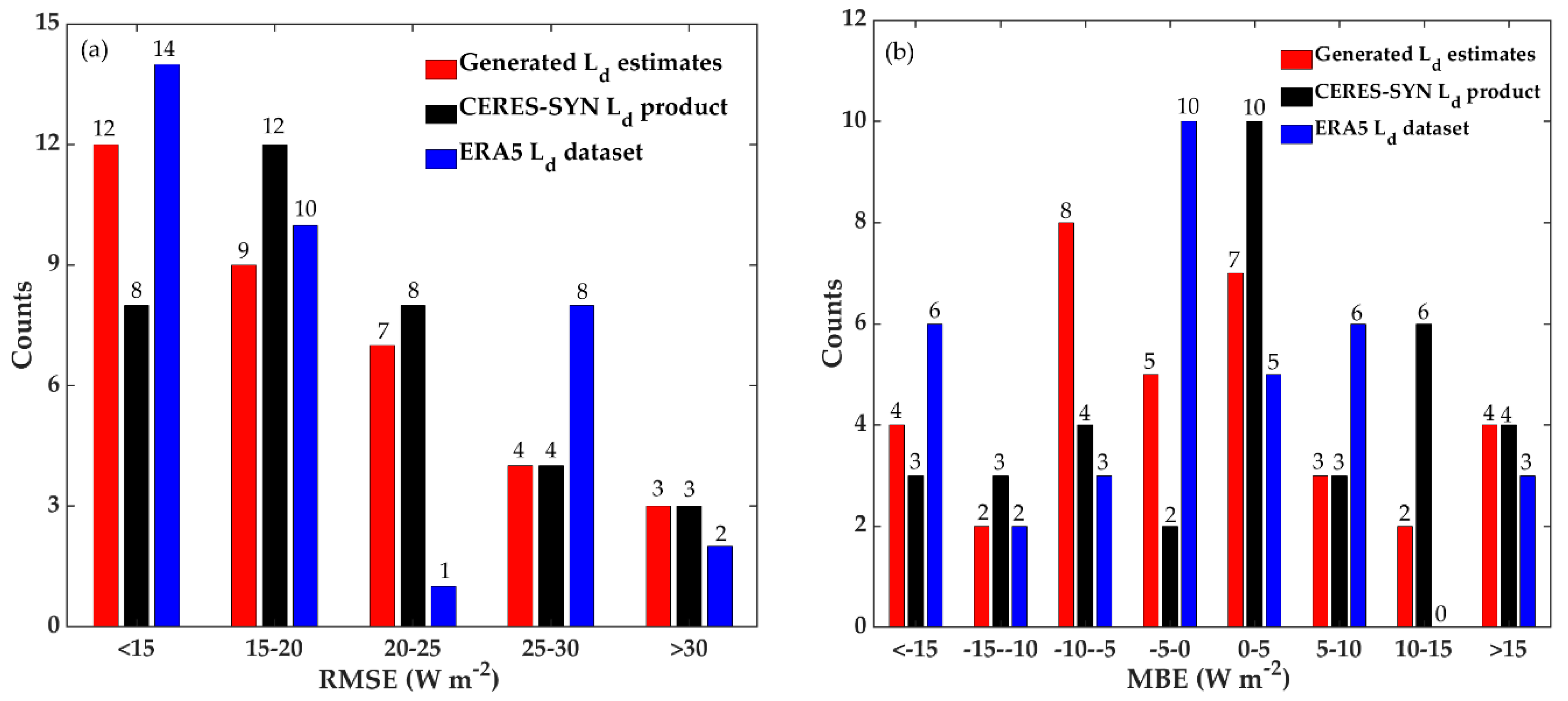
4.2. Comparison with Existing Ld Products
4.3. Spatial and Temporal Analysis of Ld
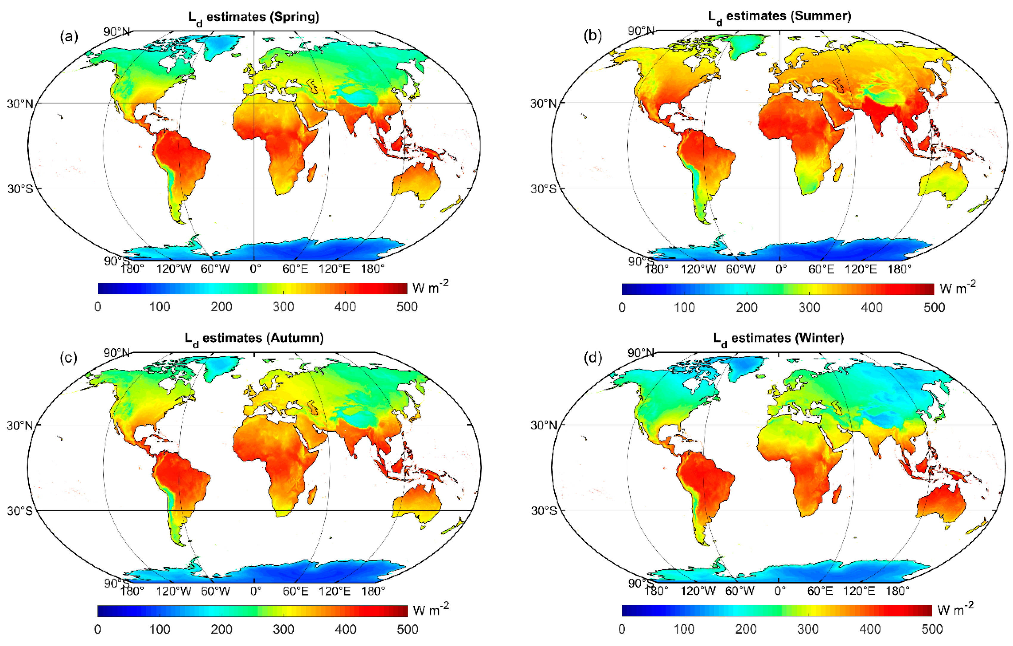
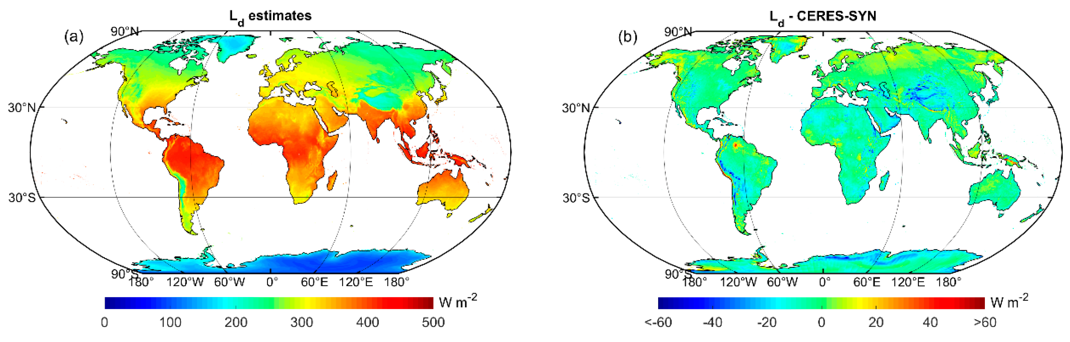
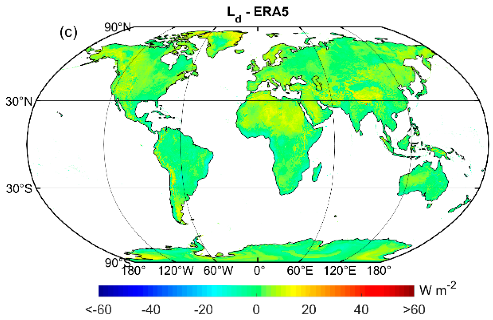
4.3.1. Spatial Distribution
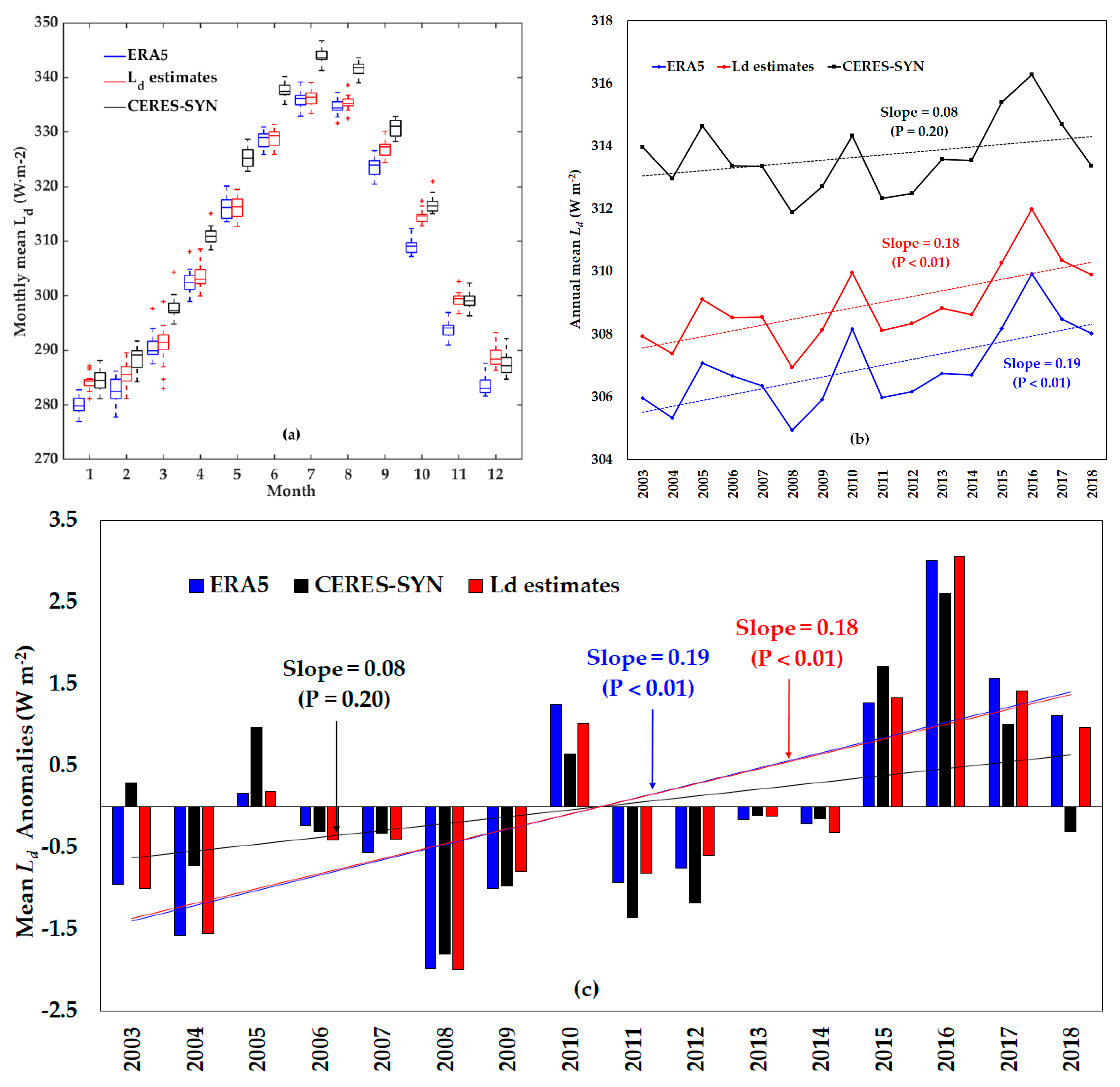
4.3.2. Time Series and Long-Term Trend
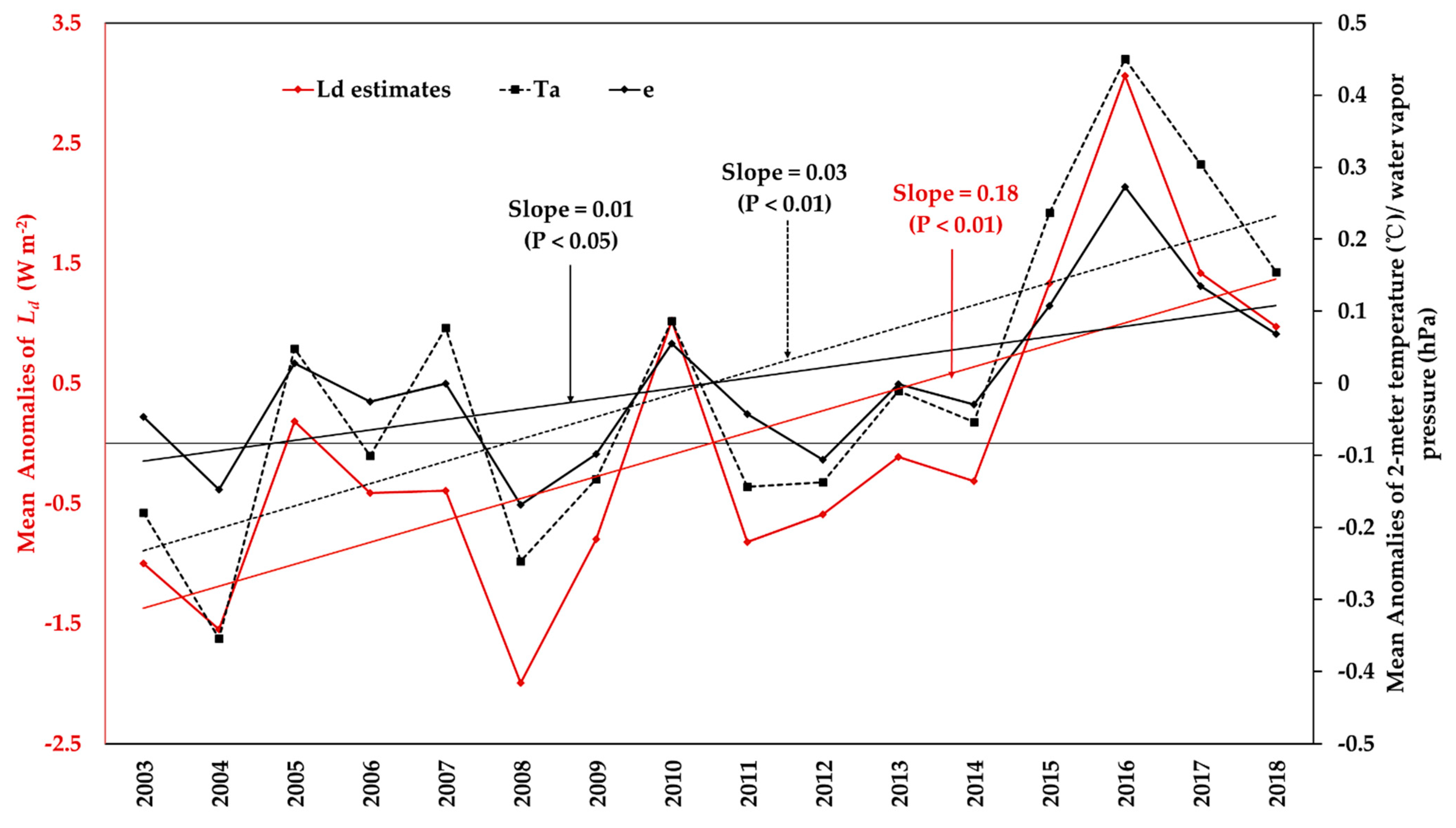
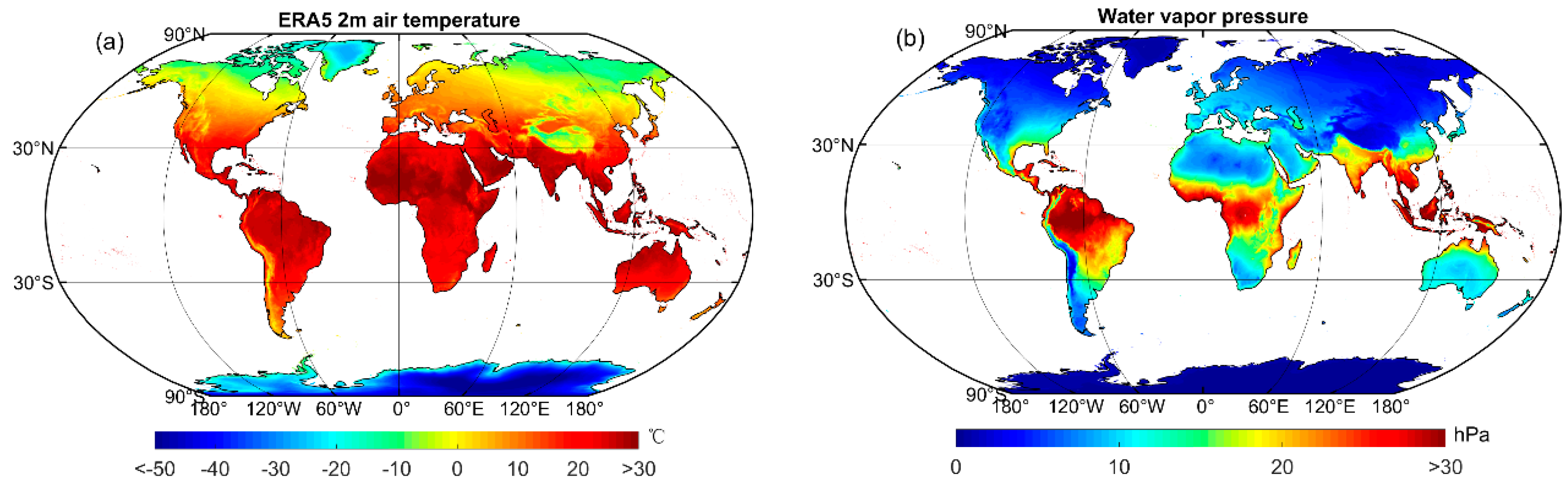
4.3.3. Relationships between the Long-Term Ld and the Key Factors
5. Discussion
5.1. Shortcomings of the GBRT Model
5.2. Accuracy and Completeness of Input Datasets and Ground Measurements
6. Conclusions
Author Contributions
Funding
Data Availability Statement
Acknowledgments
Conflicts of Interest
Appendix A

| Number | Site Code | Site Name | Latitude (deg) | Longitude (deg) | Elevation (m) | Time Period |
|---|---|---|---|---|---|---|
| 1 | BR-Npw | Northern Pantanal Wetland | −16.50 | −56.41 | 120 | 2013–2017 |
| 2 | BR-Sa3 | Santarem-Km83-Logged Forest | −3.02 | −54.97 | 100 | 2001–2004 |
| 3 | CA-ARF | Attawapiskat River Fen | 52.70 | −83.96 | 88 | 2011–2015 |
| 4 | CA-Ca1 | British Columbia–1949 Douglas-fir stand | 49.87 | −125.33 | 300 | 2000–2010 |
| 5 | CA-Ca3 | British Columbia–Pole sapling Douglas-fir stand | 49.53 | −124.90 | \ | 2002–2016 |
| 6 | CA-Cbo | Ontario–Mixed Deciduous, Borden Forest Site | 44.32 | −79.93 | 120 | 2005–2018 |
| 7 | CA-DBB | Delta Burns Bog | 49.13 | −122.98 | 4 | 2016–2018 |
| 8 | CA-Gro | Ontario–Groundhog River, Boreal Mixedwood Forest | 48.22 | −82.16 | 340 | 2003–2014 |
| 9 | CA-Na1 | New Brunswick–1967 Balsam Fir–Nashwaak Lake Site 01 (Mature balsam fir forest) | 46.47 | −67.10 | 341 | 2003–2005 |
| 10 | CA-Oas | Saskatchewan–Western Boreal, Mature Aspen | 53.63 | −106.20 | 530 | 2000–2010 |
| 11 | CA-Obs | Saskatchewan–Western Boreal, Mature Black Spruce | 53.99 | −105.12 | 628.94 | 2000–2010 |
| 12 | CA-Ojp | Saskatchewan–Western Boreal, Mature Jack Pine | 53.92 | −104.69 | 579 | 2000–2010 |
| 13 | CA-Qcu | Quebec–Eastern Boreal, Black Spruce/Jack Pine Cutover | 49.27 | −74.04 | 392.3 | 2004–2010 |
| 14 | CA-Qfo | Quebec–Eastern Boreal, Mature Black Spruce | 49.69 | −74.34 | 382 | 2003–2010 |
| 15 | CA-SCB | Scotty Creek Bog | 61.31 | −121.30 | 280 | 2014–2017 |
| 16 | CA-SCC | Scotty Creek Landscape | 61.31 | −121.30 | 285 | 2013–2016 |
| 17 | CA-SF1 | Saskatchewan–Western Boreal, forest burned in 1977 | 54.49 | −105.82 | 536 | 2003–2006 |
| 18 | CA-SF2 | Saskatchewan–Western Boreal, forest burned in 1989 | 54.25 | −105.88 | 520 | 2002–2005 |
| 19 | CA-SF3 | Saskatchewan–Western Boreal, forest burned in 1998 | 54.09 | −106.01 | 540 | 2002–2006 |
| 20 | CA-SJ1 | Saskatchewan–Western Boreal, Jack Pine forest harvested in 1994 | 53.91 | −104.66 | 580 | 2001–2010 |
| 21 | CA-SJ2 | Saskatchewan–Western Boreal, Jack Pine forest harvested in 2002 | 53.95 | −104.65 | 580 | 2003–2010 |
| 22 | CA-SJ3 | Saskatchewan–Western Boreal, Jack Pine forest harvested in 1975 (BOREAS Young Jack Pine) | 53.88 | −104.65 | \ | 2004–2010 |
| 23 | CA-TP4 | Ontario–Turkey Point 1939 Plantation White Pine | 42.71 | −80.36 | 184 | 2003–2017 |
| 24 | CA-TPD | Ontario–Turkey Point Mature Deciduous | 42.64 | −80.56 | 260 | 2012–2017 |
| 25 | CA-WP1 | Alberta–Western Peatland–LaBiche River,Black Spruce/Larch Fen | 54.95 | −112.47 | 540 | 2003–2009 |
| 26 | US-A03 | ARM-AMF3-Oliktok | 70.50 | −149.88 | 5 | 2014–2018 |
| 27 | US-A10 | ARM-NSA-Barrow | 71.32 | −156.61 | 4 | 2011–2018 |
| 28 | US-A32 | ARM-SGP Medford hay pasture | 36.82 | −97.82 | 335 | 2015–2017 |
| 29 | US-A74 | ARM SGP milo field | 36.81 | −97.55 | 337 | 2016–2017 |
| 30 | US-AR1 | ARM USDA UNL OSU Woodward Switchgrass 1 | 36.43 | −99.42 | 611 | 2009–2012 |
| 31 | US-AR2 | ARM USDA UNL OSU Woodward Switchgrass 2 | 36.64 | −99.60 | 646 | 2009–2012 |
| 32 | US-ARM | ARM Southern Great Plains site- Lamont | 36.61 | −97.49 | 314 | 2003–2018 |
| 33 | US-An1 | Anaktuvuk River Severe Burn | 68.99 | −150.28 | 600 | 2008–2009 |
| 34 | US-An2 | Anaktuvuk River Moderate Burn | 68.95 | −150.21 | 600 | 2008–2019 |
| 35 | US-An3 | Anaktuvuk River Unburned | 68.93 | −150.27 | 600 | 2008–2010 |
| 36 | US-Bi1 | Bouldin Island Alfalfa | 38.10 | −121.50 | −2.7 | 2016–2018 |
| 37 | US-Bi2 | Bouldin Island corn | 38.11 | −121.54 | −5 | 2017–2018 |
| 38 | US-Bkg | Brookings | 44.35 | −96.84 | 510 | 2004–2010 |
| 39 | US-Blk | Black Hills | 44.16 | −103.65 | 1718 | 2004–2008 |
| 40 | US-Bo1 | Bondville | 40.01 | −88.29 | 219 | 2000–2008 |
| 41 | US-Br1 | Brooks Field Site 10- Ames | 41.97 | −93.69 | 313 | 2005–2011 |
| 42 | US-Br3 | Brooks Field Site 11- Ames | 41.97 | −93.69 | 313 | 2005–2011 |
| 43 | US-CPk | Chimney Park | 41.07 | −106.12 | 2750 | 2009–2013 |
| 44 | US-ChR | Chestnut Ridge | 35.93 | −84.33 | 286 | 2005–2010 |
| 45 | US-Ctn | Cottonwood | 43.95 | −101.85 | 744 | 2006–2009 |
| 46 | US-Dia | Diablo | 37.68 | −121.53 | 323 | 2010–2012 |
| 47 | US-Dk1 | Duke Forest-open field | 35.97 | −79.09 | 168 | 2004–2008 |
| 48 | US-Dk2 | Duke Forest-hardwoods | 35.97 | −79.10 | 168 | 2004–2008 |
| 49 | US-Dk3 | Duke Forest–loblolly pine | 35.98 | −79.09 | 163 | 2004–2008 |
| 50 | US-EDN | Eden Landing Ecological Reserve | 37.62 | −122.11 | \ | 2018 |
| 51 | US-EML | Eight Mile Lake Permafrost thaw gradient, Healy Alaska. | 63.88 | −149.25 | 700 | 2011–2018 |
| 52 | US-FPe | Fort Peck | 48.31 | −105.10 | 634 | 2000–2008 |
| 53 | US-FR2 | Freeman Ranch- Mesquite Juniper | 29.95 | −98.00 | 271.9 | 2008 |
| 54 | US-FR3 | Freeman Ranch- Woodland | 29.94 | −97.99 | 232 | 2008–2012 |
| 55 | US-Fmf | Flagstaff–Managed Forest | 35.14 | −111.73 | 2160 | 2005–2010 |
| 56 | US-Fuf | Flagstaff–Unmanaged Forest | 35.09 | −111.76 | 2180 | 2005–2010 |
| 57 | US-Fwf | Flagstaff–Wildfire | 35.45 | −111.77 | 2270 | 2005–2010 |
| 58 | US-GLE | GLEES | 41.37 | −106.24 | 3197 | 2004–2018 |
| 59 | US-Goo | Goodwin Creek | 34.25 | −89.87 | 87 | 2002–2006 |
| 60 | US-HBK | Hubbard Brook Experimental Forest | 43.94 | −71.72 | 367 | 2017–2018 |
| 61 | US-HRA | Humnoke Farm Rice Field–Field A | 34.59 | −91.75 | \ | 2016–2017 |
| 62 | US-HRC | Humnoke Farm Rice Field–Field C | 34.59 | −91.75 | \ | 2016–2017 |
| 63 | US-Ha2 | Harvard Forest Hemlock Site | 42.54 | −72.18 | 360 | 2014–2018 |
| 64 | US-Hn3 | Hobcaw Barony Longleaf Pine Restoration | 46.69 | −119.46 | 120.9 | 2017–2018 |
| 65 | US-Ho1 | Howland Forest (main tower) | 45.20 | −68.74 | 60 | 2007–2018 |
| 66 | US-Ho2 | Howland Forest (west tower) | 45.21 | −68.75 | 61 | 2007–2009 |
| 67 | US-Ho3 | Howland Forest (harvest site) | 45.21 | −68.73 | 61 | 2007–2009 |
| 68 | US-Ivo | Ivotuk | 68.49 | −155.75 | 568 | 2003–2006 |
| 69 | US-KFS | Kansas Field Station | 39.06 | −95.19 | 310 | 2008–2018 |
| 70 | US-KLS | Kansas Land Institute | 38.77 | −97.57 | 373 | 2012–2017 |
| 71 | US-KM4 | KBS Marshall Farms Smooth Brome Grass (Ref) | 42.44 | −85.33 | 288 | 2010–2018 |
| 72 | US-KS3 | Kennedy Space Center (salt marsh) | 28.71 | −80.74 | 0 | 2018 |
| 73 | US-KUT | KUOM Turfgrass Field | 44.99 | −93.19 | 301 | 2006–2009 |
| 74 | US-Kon | Konza Prairie LTER (KNZ) | 39.08 | −96.56 | 417 | 2006–2018 |
| 75 | US-Los | Lost Creek | 46.08 | −89.98 | 480 | 2014–2018 |
| 76 | US-MMS | Morgan Monroe State Forest | 39.32 | −86.41 | 275 | 2000–2018 |
| 77 | US-MOz | Missouri Ozark Site | 38.74 | −92.20 | 219.4 | 2004–2017 |
| 78 | US-MRf | Mary’s River (Fir) site | 44.65 | −123.55 | 263 | 2007–2011 |
| 79 | US-MSR | Montana Sun River winter wheat | 47.48 | −111.72 | 1110 | 2016 |
| 80 | US-Me2 | Metolius mature ponderosa pine | 44.45 | −121.56 | 1253 | 2005–2018 |
| 81 | US-Me3 | Metolius-second young aged pine | 44.32 | −121.61 | 1005 | 2009 |
| 82 | US-Me6 | Metolius Young Pine Burn | 44.32 | −121.61 | 998 | 2010–2018 |
| 83 | US-Men | Lake Mendota, Center for Limnology Site | 43.08 | −89.40 | 260 | 2012–2018 |
| 84 | US-Mpj | Mountainair Pinyon-Juniper Woodland | 34.44 | −106.24 | 2196 | 2008–2018 |
| 85 | US-MtB | Mt Bigelow | 32.42 | −110.73 | 2573 | 2009–2018 |
| 86 | US-NC1 | Mt Bigelow | 35.81 | −76.71 | 5 | 2005–2012 |
| 87 | US-NC2 | NC_Loblolly Plantation | 35.80 | −76.67 | 5 | 2005–2018 |
| 88 | US-NC3 | NC_Clearcut#3 | 35.80 | −76.66 | 5 | 2013–2018 |
| 89 | US-NC4 | NC_AlligatorRiver | 35.79 | −75.90 | 1 | 2015–2018 |
| 90 | US-NGB | NGEE Arctic Barrow | 71.28 | −156.61 | 5.273 | 2012–2018 |
| 91 | US-NGC | NGEE Arctic Council | 64.86 | −163.70 | 35 | 2017–2018 |
| 92 | US-NR1 | Niwot Ridge Forest (LTER NWT1) | 40.03 | −105.55 | 3050 | 2000–2018 |
| 93 | US-Ne1 | Mead–irrigated continuous maize site | 41.17 | −96.48 | 361 | 2001–2018 |
| 94 | US-Ne2 | Mead–irrigated maize-soybean rotation site | 41.16 | −96.47 | 362 | 2001–2018 |
| 95 | US-Ne3 | Mead–rainfed maize-soybean rotation site | 41.18 | −96.44 | 363 | 2001–2018 |
| 96 | US-Orv | Olentangy River Wetland Research Park | 40.02 | −83.02 | 221 | 2011–2016 |
| 97 | US-Oho | Oak Openings | 41.55 | −83.84 | 230 | 2004–2013 |
| 98 | US-PHM | Plum Island High Marsh | 42.74 | −70.83 | 1.4 | 2013–2018 |
| 99 | US-Pnp | Lake Mendota, Picnic Point Site | 43.09 | −89.42 | 260 | 2016–2018 |
| 100 | US-Prr | Poker Flat Research Range Black Spruce Forest | 65.12 | −147.49 | 210 | 2010–2016 |
| 101 | US-Rls | RCEW Low Sagebrush | 43.14 | −116.74 | 1608 | 2014–2018 |
| 102 | US-Rms | RCEW Mountain Big Sagebrush | 43.06 | −116.75 | 2111 | 2014–2018 |
| 103 | US-Ro1 | Rosemount- G21 | 44.71 | −93.09 | 260 | 2004–2016 |
| 104 | US-Ro2 | Rosemount- C7 | 44.73 | −93.09 | 292 | 2015–2016 |
| 105 | US-Ro4 | Rosemount Prairie | 44.68 | −93.07 | 274 | 2015–2018 |
| 106 | US-Ro5 | Rosemount I18_South | 44.69 | −93.06 | 283 | 2017–2018 |
| 107 | US-Ro6 | Rosemount I18_North | 44.69 | −93.06 | 282 | 2017–2018 |
| 108 | US-Rpf | Poker Flat Research Range: Succession from fire scar to deciduous forest | 65.12 | −147.43 | 497 | 2013–2018 |
| 109 | US-Rwe | RCEW Reynolds Mountain East | 43.07 | −116.76 | 2098 | 2005–2007 |
| 110 | US-Rwf | RCEW Upper Sheep Prescibed Fire | 43.12 | −116.72 | 1878 | 2014–2018 |
| 111 | US-Rws | Reynolds Creek Wyoming big sagebrush | 43.17 | −116.71 | 1425 | 2014–2018 |
| 112 | US-SFP | Sioux Falls Portable | 43.24 | −96.90 | 386 | 2007–2009 |
| 113 | US-SRC | Santa Rita Creosote | 31.91 | −110.84 | 950 | 2008–2014 |
| 114 | US-SRG | Santa Rita Grassland | 31.79 | −110.83 | 1291 | 2008–2018 |
| 115 | US-SRM | Santa Rita Mesquite | 31.82 | −110.87 | 1120 | 2004–2018 |
| 116 | US-Seg | Sevilleta grassland | 34.36 | −106.70 | 1622 | 2007–2018 |
| 117 | US-Ses | Sevilleta shrubland | 34.33 | −106.74 | 1604 | 2007–2018 |
| 118 | US-Skr | Shark River Slough (Tower SRS-6) Everglades | 25.36 | −81.08 | 0 | 2004–2011 |
| 119 | US-Slt | Silas Little- New Jersey | 39.91 | −74.60 | 30 | 2007–2012 |
| 120 | US-Sne | Sherman Island Restored Wetland | 38.04 | −121.75 | −5 | 2016–2018 |
| 121 | US-Snf | Sherman Barn | 38.04 | −121.73 | −4 | 2018 |
| 122 | US-Srr | Suisun marsh–Rush Ranch | 38.20 | −122.03 | 8 | 2014–2017 |
| 123 | US-Ton | Tonzi Ranch | 38.43 | −120.97 | 177 | 2014–2018 |
| 124 | US-Tw1 | Twitchell Wetland West Pond | 38.11 | −121.65 | −5 | 2011–2018 |
| 125 | US-Tw2 | Twitchell Corn | 38.10 | −121.64 | −5 | 2012–2013 |
| 126 | US-Tw3 | Twitchell Alfalfa | 38.12 | −121.65 | −4 | 2013–2018 |
| 127 | US-Tw4 | Twitchell East End Wetland | 38.10 | −121.64 | −5 | 2013–2018 |
| 128 | US-Tw5 | East Pond Wetland | 38.11 | −121.64 | −5 | 2018 |
| 129 | US-UM3 | Douglas Lake | 45.57 | −84.67 | 234 | 2013–2014 |
| 130 | US-UMB | Univ. of Mich. Biological Station | 45.56 | −84.71 | 234 | 2007–2018 |
| 131 | US-UMd | UMBS Disturbance | 45.56 | −84.70 | 239 | 2008–2018 |
| 132 | US-Uaf | University of Alaska, Fairbanks | 64.87 | −147.86 | 155 | 2009–2018 |
| 133 | US-UiA | University of Illinois Switchgrass | 40.06 | −88.20 | 224 | 2015 |
| 134 | US-Var | Vaira Ranch- Ione | 38.41 | −120.95 | 129 | 2004–2018 |
| 135 | US-Vcm | Valles Caldera Mixed Conifer | 35.89 | −106.53 | 3003 | 2009–2018 |
| 136 | US-Vcp | Valles Caldera Ponderosa Pine | 35.86 | −106.60 | 2542 | 2007–2018 |
| 137 | US-Vcs | Valles Caldera Sulphur Springs Mixed Conifer | 35.92 | −106.61 | 2752 | 2016–2018 |
| 138 | US-WBW | Walker Branch Watershed | 35.96 | −84.29 | 283 | 2001–2007 |
| 139 | US-WCr | Willow Creek | 45.81 | −90.08 | 520 | 2000–2018 |
| 140 | US-WPT | Winous Point North Marsh | 41.46 | −83.00 | 175 | 2011–2013 |
| 141 | US-Wdn | Walden | 40.78 | −106.26 | 2469 | 2006–2008 |
| 142 | US-Wgr | Willamette Grass | 45.11 | −122.66 | 52 | 2015 |
| 143 | US-Whs | Walnut Gulch Lucky Hills Shrub | 31.74 | −110.05 | 1370 | 2009–2018 |
| 144 | US-Wjs | Willard Juniper Savannah | 34.43 | −105.86 | 1931 | 2007–2018 |
| 145 | US-Wkg | Walnut Gulch Kendall Grasslands | 31.74 | −109.94 | 1531 | 2004–2018 |
| 146 | US-Wpp | Willamette Poplar | 44.14 | −123.18 | 111 | 2015 |
| 147 | US-Wrc | Wind River Crane Site | 45.82 | −121.95 | 371 | 2000–2015 |
| 148 | US-xAB | NEON Abby Road (ABBY) | 45.76 | −122.33 | 363 | 2017–2018 |
| 149 | US-xBN | NEON Caribou Creek–Poker Flats Watershed (BONA) | 65.15 | −147.50 | 263 | 2018 |
| 150 | US-xBR | NEON Bartlett Experimental Forest (BART) | 44.06 | −71.29 | 232 | 2017–2018 |
| 151 | US-xCP | NEON Central Plains Experimental Range (CPER) | 40.82 | −104.75 | 1654 | 2017–2018 |
| 152 | US-xDC | NEON Dakota Coteau Field School (DCFS) | 47.16 | −99.11 | 559 | 2017–2018 |
| 153 | US-xDJ | NEON Delta Junction (DEJU) | 63.88 | −145.75 | 529 | 2017–2018 |
| 154 | US-xDL | NEON Dead Lake (DELA) | 32.54 | −87.80 | 22 | 2017–2018 |
| 155 | US-xGR | NEON Great Smoky Mountains National Park, Twin Creeks (GRSM) | 35.69 | −83.50 | 579 | 2018 |
| 156 | US-xHA | NEON Harvard Forest (HARV) | 42.54 | −72.17 | 351 | 2017–2018 |
| 157 | US-xHE | NEON Healy (HEAL) | 63.88 | −149.21 | 705 | 2017–2018 |
| 158 | US-xJE | NEON Jones Ecological Research Center (JERC) | 31.19 | −84.47 | 44 | 2017–2018 |
| 159 | US-xJR | NEON Jornada LTER (JORN) | 32.59 | −106.84 | 1329 | 2017–2018 |
| 160 | US-xKA | NEON Konza Prairie Biological Station–Relocatable (KONA) | 39.11 | −96.61 | 1329 | 2017–2018 |
| 161 | US-xKZ | NEON Konza Prairie Biological Station (KONZ) | 39.10 | −96.56 | 381 | 2017–2018 |
| 162 | US-xNG | NEON Northern Great Plains Research Laboratory (NOGP) | 46.77 | −100.92 | 578 | 2017–2018 |
| 163 | US-xNQ | NEON Onaqui-Ault (ONAQ) | 40.18 | −112.45 | 1685 | 2017–2018 |
| 164 | US-xRM | NEON Rocky Mountain National Park, CASTNET (RMNP) | 40.28 | −105.55 | 2743 | 2017–2018 |
| 165 | US-xSE | NEON Smithsonian Environmental Research Center (SERC) | 38.89 | −76.56 | 15 | 2017–2018 |
| 166 | US-xSL | NEON North Sterling, CO (STER) | 40.46 | −103.03 | 1364 | 2017–2018 |
| 167 | US-xSP | NEON Soaproot Saddle (SOAP) | 37.03 | −119.26 | 1160 | 2017–2018 |
| 168 | US-xSR | NEON Santa Rita Experimental Range (SRER) | 31.91 | −110.84 | 983 | 2017–2018 |
| 169 | US-xST | NEON Steigerwaldt Land Services (STEI) | 45.51 | −89.59 | 481 | 2017–2018 |
| 170 | US-xTE | NEON Lower Teakettle (TEAK) | 37.01 | −119.01 | 2147 | 2018 |
| 171 | US-xTR | NEON Treehaven (TREE) | 45.49 | −89.59 | 472 | 2017–2018 |
| 172 | US-xUK | NEON The University of Kansas Field Station (UKFS) | 39.04 | −95.19 | 335 | 2017–2018 |
| 173 | US-xUN | NEON University of Notre Dame Environmental Research Center (UNDE) | 46.23 | −89.54 | 518 | 2017–2018 |
| 174 | US-xWD | NEON Woodworth (WOOD) | 47.13 | −99.24 | 579 | 2017–2018 |
| 175 | US-xWR | NEON Wind River Experimental Forest (WREF) | 45.82 | −121.95 | 407 | 2018 |
| 176 | MSE | Mase paddy flux site | 36.05 | 140.03 | 13 | 2001 |
| 177 | PSO | Pasoh Forest Reserve | 2.97 | 102.31 | 75–150 | 2003–2009 |
| 178 | BKS | Bukit Soeharto | -0.86 | 117.04 | 20 | 2001–2002 |
| 179 | CBS | Changbaishan Site | 41.40 | 128.10 | 731 | 2003–2005 |
| 180 | FHK | Fuji Hokuroku Flux Observation Site | 35.44 | 138.76 | 1050–1150 | 2006–2012 |
| 181 | GCK | Gwangreung Coniferous forest | 37.75 | 127.16 | 132 | 2007–2008 |
| 182 | HBG | Haibei Potentilla fruticisa bosk Site | 37.48 | 101.20 | 756 | 2003–2004 |
| 183 | HFK | Haenam Farmland | 34.55 | 127.57 | 12 | 2008 |
| 184 | IRI | IRRI Flux Research Site | 14.14 | 121.27 | 21 | 2009–2014 |
| 185 | KBU | Kherlenbayan Ulaan | 47.21 | 108.74 | 1235 | 2003–2009 |
| 186 | LSH | Laoshan | 45.28 | 127.58 | 340 | 2002 |
| 187 | MBF | Moshiri Birch Forest Site | 44.38 | 142.32 | 585 | 2003–2005 |
| 188 | MKL | Mae Klong | 14.59 | 98.84 | 585 | 2003–2004 |
| 189 | MMF | Moshiri Mixd Forest Site | 44.32 | 142.26 | 340 | 2003–2005 |
| 190 | Palangkaraya drained forest | −2.35 | 114.04 | 30 | 2002–2005 | |
| 191 | QYZ | Qianyanzhou Site | 26.73 | 115.07 | 100 | 2003–2004 |
| 192 | SKR | Sakaerat | 14.49 | 101.92 | 543 | 2001–2003 |
| 193 | SKT | Southern Khentei Taiga | 48.35 | 108.65 | 1630 | 2003–2006 |
| 194 | SMF | Seto Mixed Forest Site | 35.26 | 137.08 | 205 | 2002–2015 |
| 195 | SWL | Suwa Lake Site | 36.05 | 138.11 | 759 | 2015–2018 |
| 196 | TKC | Takayama evergreen coniferous forest site | 36.14 | 137.37 | 800 | 2007 |
| 197 | TMK | Tomakomai Flux Research Site | 42.74 | 141.51 | 140 | 2001–2003 |
| 198 | TSE | CC-LaG Teshio Experimental Forest | 45.06 | 142.11 | 70 | 2001–2005 |
| 199 | YCS | Yuchen Site | 36.83 | 116.57 | 28 | 2003–2005 |
| 200 | YLF | Yakutsk Spasskaya Pad larch | 62.26 | 129.17 | 220 | 2003–2007 |
| 201 | YPF | Yakutsk Pine | 62.24 | 129.65 | 220 | 2004–2007 |
| 202 | ALE | Alert | 82.49 | −62.42 | 127 | 2004–2014 |
| 203 | ASP | Alice Springs | −23.80 | 133.89 | 547 | 2000–2018 |
| 204 | BAR | Barrow | 71.32 | −156.61 | 8 | 2000–2017 |
| 205 | BIL | Billings | 36.61 | −97.52 | 317 | 2000–2017 |
| 206 | BON | Bondville | 40.07 | −88.37 | 213 | 2009–2018 |
| 207 | BOS | Boulder | 40.13 | −105.24 | 1689 | 2009–2018 |
| 208 | BOU | Boulder | 40.05 | −105.01 | 1577 | 2000–2016 |
| 209 | BRB | Brasilia | −15.60 | −47.71 | 1023 | 2008–2018 |
| 210 | CAB | Cabauw | 51.97 | 4.93 | 0 | 2005–2018 |
| 211 | CAM | Camborne | 50.22 | −5.32 | 88 | 2001–2017 |
| 212 | CAR | Carpentras | 44.08 | 5.06 | 100 | 2000–2018 |
| 213 | CNR | Cener | 42.82 | −1.60 | 471 | 2009–2018 |
| 214 | COC | Cocos Island | −12.19 | 96.84 | 6 | 2004–2018 |
| 215 | DAA | De Aar | −30.67 | 23.99 | 1287 | 2000–2018 |
| 216 | DAR | Darwin | −12.43 | 130.89 | 30 | 2002–2015 |
| 217 | DOM | Concordia Station, Dome C | −75.10 | 123.38 | 3233 | 2006–2018 |
| 218 | DRA | Desert Rock | 36.63 | −116.02 | 1007 | 2009–2018 |
| 219 | DWN | Darwin Met Office | −12.42 | 130.89 | 32 | 2008–2018 |
| 220 | E13 | Southern Great Plains | 36.61 | −97.49 | 318 | 2000–2017 |
| 221 | ENA | Eastern North Atlantic | 39.09 | −28.03 | 15.2 | 2013–2015 |
| 222 | EUR | Eureka | 79.99 | −85.94 | 85 | 2007–2011 |
| 223 | FLO | Florianopolis | −27.60 | −48.52 | 11 | 2013–2018 |
| 224 | FPE | Fort Peck | 48.32 | −105.10 | 634 | 2009–2018 |
| 225 | FUA | Fukuoka | 33.58 | 130.38 | 3 | 2010–2018 |
| 226 | GAN | Gandhinagar | 23.11 | 72.63 | 65 | 2014–2015 |
| 227 | GCR | Goodwin Creek | 34.25 | −89.87 | 98 | 2009–2018 |
| 228 | GOB | Gobabeb | −23.56 | 15.04 | 407 | 2012–2018 |
| 229 | GUR | Gurgaon | 28.42 | 77.16 | 259 | 2014–2018 |
| 230 | GVN | Georg von Neumayer | −70.65 | −8.25 | 42 | 2000–2018 |
| 231 | HOW | Howrah | 22.55 | 88.31 | 51 | 2014–2018 |
| 232 | ISH | Ishigakijima | 24.34 | 124.16 | 5.7 | 2010–2018 |
| 233 | LAU | Lauder | −45.05 | 169.69 | 350 | 2000–2018 |
| 234 | LER | Lerwick | 60.14 | −1.18 | 80 | 2001–2017 |
| 235 | LIN | Lindenberg | 52.21 | 14.12 | 125 | 2000–2017 |
| 236 | LRC | Langley Research Center | 37.10 | −76.39 | 3 | 2014–2018 |
| 237 | LYU | Lanyu Station | 22.04 | 121.56 | 324 | 2018 |
| 238 | MAN | Momote | −2.06 | 147.43 | 6 | 2000–2013 |
| 239 | NAU | Nauru Island | −0.52 | 166.92 | 7 | 2000–2013 |
| 240 | NEW | Newcastle | −32.88 | 151.73 | 18.5 | 2017–2018 |
| 241 | NYA | Ny-Ålesund | 78.93 | 11.93 | 11 | 2000–2018 |
| 242 | PAL | Palaiseau, SIRTA Observatory | 48.71 | 2.21 | 156 | 2003–2018 |
| 243 | PAY | Payerne | 46.82 | 6.94 | 491 | 2000–2018 |
| 244 | PSU | Rock Springs | 40.72 | −77.93 | 376 | 2009–2018 |
| 245 | PTR | Petrolina | −9.07 | −40.32 | 387 | 2008–2018 |
| 246 | REG | Regina | 50.21 | −104.71 | 578 | 2000–2011 |
| 247 | SAP | Sapporo | 43.06 | 141.33 | 17.2 | 2010–2018 |
| 248 | SBO | Sede Boqer | 30.86 | 34.78 | 500 | 2003–2012 |
| 249 | SMS | São Martinho da Serra | −29.44 | −53.82 | 489 | 2008–2017 |
| 250 | SON | Sonnblick | 47.05 | 12.96 | 3108.9 | 2013–2018 |
| 251 | SOV | Solar Village | 24.91 | 46.41 | 650 | 2000–2002 |
| 252 | SXF | Sioux Falls | 43.73 | −96.62 | 473 | 2009–2018 |
| 253 | SYO | Syowa | −69.01 | 39.59 | 18 | 2000–2018 |
| 254 | TAM | Tamanrasset | 22.79 | 5.53 | 1385 | 2000–2018 |
| 255 | TAT | Tateno | 36.06 | 140.13 | 25 | 2000–2018 |
| 256 | TIR | Tiruvallur | 13.09 | 79.97 | 36 | 2014–2018 |
| 257 | TOR | Toravere | 58.25 | 26.46 | 70 | 2003–2018 |
| 258 | XIA | Xianghe | 39.75 | 116.96 | 32 | 2005–2015 |
| 259 | AT-Neu | Neustift | 47.12 | 11.32 | 970 | 2005–2012 |
| 260 | AU-ASM | Alice Springs | −22.28 | 133.25 | \ | 2010–2014 |
| 261 | AU-Ade | Adelaide River | −13.08 | 131.12 | \ | 2007–2009 |
| 262 | AU-Cpr | Calperum | −34.00 | 140.59 | \ | 2010–2014 |
| 263 | AU-Cum | Cumberland Plain | −33.62 | 150.72 | \ | 2012–2014 |
| 264 | AU-DaP | Daly River Savanna | −14.06 | 131.32 | \ | 2007–2013 |
| 265 | AU-DaS | Daly River Cleared | −14.16 | 131.39 | \ | 2008–2014 |
| 266 | AU-Dry | Dry River | −15.26 | 132.37 | \ | 2008–2014 |
| 267 | AU-Emr | Emerald | −23.86 | 148.47 | \ | 2011–2013 |
| 268 | AU-Fog | Fogg Dam | −12.55 | 131.31 | \ | 2006–2008 |
| 269 | AU-GWW | Great Western Woodlands, Western Australia, Australia | −30.19 | 120.65 | \ | 2013–2014 |
| 270 | AU-Gin | Gingin | −31.38 | 115.71 | \ | 2011–2014 |
| 271 | AU-Lox | Loxton | −34.47 | 140.66 | \ | 2008–2009 |
| 272 | AU-RDF | Red Dirt Melon Farm, Northern Territory | −14.56 | 132.48 | \ | 2011–2013 |
| 273 | AU-Rig | Riggs Creek | −36.65 | 145.58 | \ | 2011–2014 |
| 274 | AU-Rob | Robson Creek, Queensland, Australia | −17.12 | 145.63 | \ | 2014 |
| 275 | AU-Stp | Sturt Plains | −17.15 | 133.35 | \ | 2008–2014 |
| 276 | AU-TTE | Ti Tree East | −22.29 | 133.64 | \ | 2012–2014 |
| 277 | AU-Tum | Tumbarumba | −35.66 | 148.15 | 1200 | 2007–2014 |
| 278 | AU-Whr | Whroo | −36.67 | 145.03 | \ | 2011–2014 |
| 279 | AU-Wom | Wombat | −37.42 | 144.09 | 705 | 2010–2014 |
| 280 | AU-Ync | Jaxa | −34.99 | 146.29 | \ | 2012–2014 |
| 281 | BE-Bra | Brasschaat | 51.31 | 4.52 | 16 | 2007–2014 |
| 282 | BE-Lon | Lonzee | 50.55 | 4.75 | 167 | 2005–2014 |
| 283 | CH-Cha | Chamau | 47.21 | 8.41 | 393 | 2005–2014 |
| 284 | CH-Dav | Davos | 46.82 | 9.86 | 1639 | 2006–2014 |
| 285 | CH-Fru | Früebüel | 47.12 | 8.54 | 982 | 2005–2014 |
| 286 | CH-Lae | Laegern | 47.48 | 8.36 | 689 | 2005–2014 |
| 287 | CH-Oe1 | Oensingen grassland | 47.29 | 7.73 | 450 | 2003–2008 |
| 288 | CH-Oe2 | Oensingen crop | 47.29 | 7.73 | 452 | 2004–2014 |
| 289 | CN-Cha | Changbaishan | 42.40 | 128.10 | \ | 2003–2005 |
| 290 | CN-Cng | Changling | 44.59 | 123.51 | \ | 2007–2010 |
| 291 | CN-Dan | Dangxiong | 30.50 | 91.07 | \ | 2004–2005 |
| 292 | CN-Din | Dinghushan | 23.17 | 112.54 | \ | 2003–2005 |
| 293 | CN-Ha2 | Haibei Shrubland | 37.61 | 101.33 | \ | 2003–2005 |
| 294 | CN-Qia | Qianyanzhou | 26.74 | 115.06 | \ | 2003–2005 |
| 295 | CZ-wet | Trebon (CZECHWET) | 49.02 | 14.77 | 426 | 2006–2014 |
| 296 | DE-Akm | Anklam | 53.87 | 13.68 | −1 | 2009–2014 |
| 297 | DE-Geb | Gebesee | 51.10 | 10.91 | 161.5 | 2001–2014 |
| 298 | DE-Gri | Grillenburg | 50.95 | 13.51 | 385 | 2006–2014 |
| 299 | DE-Hai | Hainich | 51.08 | 10.45 | 430 | 2002–2012 |
| 300 | DE-Kli | Klingenberg | 50.89 | 13.52 | 478 | 2004–2014 |
| 301 | DE-Lkb | Lackenberg | 49.10 | 13.30 | 1308 | 2009–2013 |
| 302 | DE-Lnf | Leinefelde | 51.33 | 10.37 | 451 | 2002–2012 |
| 303 | DE-Obe | Oberbärenburg | 50.79 | 13.72 | 734 | 2008–2014 |
| 304 | DE-RuR | Rollesbroich | 50.62 | 6.30 | 514.7 | 2011–2014 |
| 305 | DE-RuS | Selhausen Juelich | 50.87 | 6.45 | 102.755 | 2011–2014 |
| 306 | DE-SfN | Schechenfilz Nord | 47.81 | 11.33 | 590 | 2012–2014 |
| 307 | DE-Spw | Spreewald | 51.89 | 14.03 | 61 | 2010–2014 |
| 308 | DE-Tha | Tharandt | 50.96 | 13.57 | 385 | 2004–2014 |
| 309 | DE-Zrk | Zarnekow | 53.88 | 12.89 | 0 | 2013–2014 |
| 310 | FI-Hyy | Hyytiala | 61.85 | 24.29 | 181 | 2009–2014 |
| 311 | FI-Lom | Lompolojankka | 68.00 | 24.21 | 274 | 2007–2009 |
| 312 | FR-Gri | Grignon | 48.84 | 1.95 | 125 | 2004–2014 |
| 313 | FR-LBr | Le Bray | 44.72 | −0.77 | 61 | 2003–2008 |
| 314 | FR-Pue | Puechabon | 43.74 | 3.60 | 270 | 2005–2014 |
| 315 | IT-BCi | Borgo Cioffi | 40.52 | 14.96 | 20 | 2006–2011 |
| 316 | IT-CA1 | Castel d’Asso1 | 42.38 | 12.03 | 200 | 2011–2014 |
| 317 | IT-CA2 | Castel d’Asso2 | 42.38 | 12.03 | 200 | 2011–2014 |
| 318 | IT-CA3 | Castel d’Asso3 | 42.38 | 12.02 | 197 | 2011–2014 |
| 319 | IT-Col | Collelongo | 41.85 | 13.59 | 1560 | 2004–2014 |
| 320 | IT-Isp | Ispra ABC-IS | 45.81 | 8.63 | 210 | 2013–2014 |
| 321 | IT-La2 | Lavarone2 | 45.95 | 11.29 | 1350 | 2000–2002 |
| 322 | IT-Lav | Lavarone | 45.96 | 11.28 | 1353 | 2003–2004 |
| 323 | IT-MBo | Monte Bondone | 46.01 | 11.05 | 1550 | 2003–2013 |
| 324 | IT-Noe | Arca di Noe–Le Prigionette | 40.61 | 8.15 | 25 | 2004–2014 |
| 325 | IT-Ren | Renon | 46.59 | 11.43 | 1730 | 2003–2013 |
| 326 | IT-Ro2 | Roccarespampani 2 | 42.39 | 11.92 | 160 | 2010–2012 |
| 327 | IT-SR2 | San Rossore 2 | 43.73 | 10.29 | 4 | 2013–2014 |
| 328 | IT-SRo | San Rossore | 43.73 | 10.28 | 6 | 2004–2008 |
| 329 | IT-Tor | Torgnon | 45.84 | 7.58 | 2160 | 2008–2014 |
| 330 | JP-MBF | Moshiri Birch Forest Site | 44.39 | 142.32 | \ | 2003–2005 |
| 331 | NL-Hor | Horstermeer | 52.24 | 5.07 | 2.2 | 2004–2011 |
| 332 | NL-Loo | Loobos | 52.17 | 5.74 | 25 | 2000–2014 |
| 333 | RU-Che | Cherski | 68.61 | 161.34 | 6 | 2002–2005 |
| 334 | RU-Fyo | Fyodorovskoye | 56.46 | 32.92 | 265 | 2000–2014 |
| 335 | SE-St1 | Stordalen grassland | 68.35 | 19.05 | 351 | 2012–2014 |
| 336 | SJ-Blv | Bayelva, Spitsbergen | 78.92 | 11.83 | 25 | 2008–2009 |
| 337 | US-CRT | Curtice Walter-Berger cropland | 41.63 | −83.35 | 180 | 2011–2013 |
| 338 | US-GBT | GLEES Brooklyn Tower | 41.37 | −106.24 | 3191 | 2000–2006 |
| 339 | US-Syv | Sylvania Wilderness Area | 46.24 | −89.35 | 540 | 2012–2014 |
| 340 | US-Tw4 | Twitchell East End Wetland | 38.10 | −121.64 | −5 | 2013–2014 |
| 341 | ZA-Kru | Skukuza | −25.02 | 31.50 | 359 | 2000–2003 |
| 342 | ZM-Mon | Mongu | −15.44 | 23.25 | 1053 | 2000–2009 |
| 343 | BND | Bondville | 40.05 | −88.37 | 230 | 2000–2018 |
| 344 | DRA | Desert Rock | 36.62 | −116.02 | 1007 | 2000–2018 |
| 345 | FPK | Fort Peck | 48.31 | −105.10 | 634 | 2000–2018 |
| 346 | GWN | Goodwin Creek | 34.25 | −89.87 | 98 | 2000–2018 |
| 347 | PSU | Penn State | 40.72 | −77.93 | 376 | 2000–2018 |
| 348 | SXF | Sioux Falls | 43.73 | −96.62 | 473 | 2003–2018 |
| 349 | TBL | Table Mountain | 40.13 | −105.24 | 1689 | 2000–2018 |
| Algorithm A1. The Gradient Boosting Regression Tree Algorithm. |
| Initialize |
| For do |
| For do |
| Compute the negative gradient |
| End |
| Fit a regression tree to predict the targets from covariates xi for all training dataset |
| Compute a gradient descent step size as |
| Update the model as |
| End |
| Output the final model |
References
- Oke, T.R. Boundary Layer Climates, 2nd ed.; Routledge: London, UK, 1996; p. 435. [Google Scholar]
- Udo, S.O. Quantification of solar heating of the dome of a pyrgeometer for a tropical location: Ilorin, Nigeria. J Atmos. Ocean Tech. 2000, 17, 995–1000. [Google Scholar] [CrossRef]
- Sridhar, V.; Elliott, R.L. On the development of a simple downwelling longwave radiation scheme. Agr. For. Meteorol. 2002, 112, 237–243. [Google Scholar] [CrossRef]
- Duarte, H.F.; Dias, N.L.; Maggiotto, S.R. Assessing daytime downward longwave radiation estimates for clear and cloudy skies in Southern Brazil. Agric. For. Meteorol. 2006, 139, 171–181. [Google Scholar] [CrossRef]
- Wang, K.C.; Liang, S.L. Global atmospheric downward longwave radiation over land surface under all-sky conditions from 1973 to 2008. J. Geophys. Res.-Atmos. 2009, 114. [Google Scholar] [CrossRef]
- Wild, M. The global energy balance as represented in CMIP6 climate models. Clim. Dyn. 2020, 55, 553–577. [Google Scholar] [CrossRef]
- Wild, M.; Folini, D.; Hakuba, M.Z.; Schar, C.; Seneviratne, S.I.; Kato, S.; Rutan, D.; Ammann, C.; Wood, E.F.; Konig-Langlo, G. The energy balance over land and oceans: An assessment based on direct observations and CMIP5 climate models. Clim. Dyn. 2015, 44, 3393–3429. [Google Scholar] [CrossRef]
- Wild, M.; Folini, D.; Schar, C.; Loeb, N.; Dutton, E.G.; Konig-Langlo, G. The global energy balance from a surface perspective. Clim. Dyn. 2013, 40, 3107–3134. [Google Scholar] [CrossRef]
- Morcrette, J.J. Radiation and cloud radiative properties in the European center for medium range weather forecasts forecasting system. J. Geophys. Res.-Atmos. 1991, 96, 9121–9132. [Google Scholar] [CrossRef]
- Silber, I.; Verlinde, J.; Wang, S.H.; Bromwich, D.H.; Fridlind, A.M.; Cadeddu, M.; Eloranta, E.W.; Flynn, C.J. Cloud influence on ERA5 and AMPS surface downwelling longwave radiation biases in West Antarctica. J. Clim. 2019, 32, 7935–7949. [Google Scholar] [CrossRef]
- Tang, W.; Qin, J.; Yang, K.; Zhu, F.; Zhou, X. Does ERA5 outperform satellite products in estimating atmospheric downward longwave radiation at the surface? Atmos. Res. 2021, 105453. [Google Scholar] [CrossRef]
- Zeppetello, L.R.V.; Donohoe, A.; Battisti, D.S. Does surface temperature respond to or determine downwelling longwave radiation? Geophys. Res. Lett. 2019, 46, 2781–2789. [Google Scholar] [CrossRef]
- Lhomme, J.P.; Vacher, J.J.; Rocheteau, A. Estimating downward long-wave radiation on the Andean Altiplano. Agr. For. Meteorol. 2007, 145, 139–148. [Google Scholar] [CrossRef]
- Brunt, D. Notes on radiation in the atmosphere. Q. J. R. Meteorol. Soc. 1932, 58, 389–420. [Google Scholar] [CrossRef]
- Brutsaert, W. Derivable formula for long-wave radiation from clear skies. Water Resour. Res. 1975, 11, 742–744. [Google Scholar] [CrossRef]
- Idso, S.B. A set of equations for full spectrum and 8-MU-M to 14-MU-M and 10.5-MU-M to 12.5-MU-M thermal-radiation from cloudless skies. Water Resour. Res. 1981, 17, 295–304. [Google Scholar] [CrossRef]
- Malek, E. Evaluation of effective atmospheric emissivity and parameterization of cloud at local scale. Atmos. Res. 1997, 45, 41–54. [Google Scholar] [CrossRef]
- Iziomon, M.G.; Mayer, H.; Matzarakis, A. Downward atmospheric longwave irradiance under clear and cloudy skies: Measurement and parameterization. J. Atmos. Solar Terr. Phys. 2003, 65, 1107–1116. [Google Scholar] [CrossRef]
- Jin, X.; Barber, D.; Papakyriakou, T. A new clear-sky downward longwave radiative flux parameterization for Arctic areas based on rawinsonde data. J. Geophys. Res.-Atmos. 2006, 111. [Google Scholar] [CrossRef]
- Wu, H.R.; Zhang, X.T.; Liang, S.L.; Yang, H.; Zhou, G.Q. Estimation of clear-sky land surface longwave radiation from MODIS data products by merging multiple models. J. Geophys. Res.-Atmos. 2012, 117. [Google Scholar] [CrossRef]
- Pinker, R.T.; Ewing, J.A. Modeling surface solar-radiation model formulation and validation. J. Clim. Appl. Meteorol. 1985, 24, 389–401. [Google Scholar] [CrossRef]
- Dedieu, G.; Deschamps, P.Y.; Kerr, Y.H. Satellite estimation of solar irradiance at the surface of the earth and of surface albedo using a physical model applied to meteosat data. J. Clim. Appl. Meteorol. 1987, 26, 79–87. [Google Scholar] [CrossRef]
- Duguay, C.R. An approach to the estimation of surface net-radiation in mountain areas using remote-sensing and digital terrain data. Appl. Clim. 1995, 52, 55–68. [Google Scholar] [CrossRef]
- Lee, H.T.; Ellingson, R.G. Development of a nonlinear statistical method for estimating the downward longwave radiation at the surface from satellite observations. J. Atmos. Ocean. Tech. 2002, 19, 1500–1515. [Google Scholar] [CrossRef]
- Tang, B.; Li, Z.L. Estimation of instantaneous net surface longwave radiation from MODIS cloud-free data. Remote Sens. Environ. 2008, 112, 3482–3492. [Google Scholar] [CrossRef]
- Wang, J.; Tang, B.H.; Zhang, X.Y.; Wu, H.; Li, Z.L. Estimation of surface longwave radiation over the tibetan plateau region using MODIS data for cloud-free skies. IEEE J. STARS 2014, 7, 3695–3703. [Google Scholar] [CrossRef]
- Wang, W.H.; Liang, S.L. Estimation of high-spatial resolution clear-sky longwave downward and net radiation over land surfaces from MODIS data. Remote. Sens. Environ. 2009, 113, 745–754. [Google Scholar] [CrossRef]
- Wang, W.H.; Liang, S.L. A method for estimating clear-sky instantaneous land-surface longwave radiation with GOES sounder and GOES-R ABI Data. IEEE. Geosci. Remote. Sens. Lett. 2010, 7, 708–712. [Google Scholar] [CrossRef]
- Takara, E.E.; Ellingson, R.G. Broken cloud field longwave-scattering effects. J. Atmos. Sci. 2000, 57, 1298–1310. [Google Scholar] [CrossRef]
- Yang, F.; Cheng, J. A framework for estimating cloudy sky surface downward longwave radiation from the derived active and passive cloud property parameters. Remote. Sens. Env. 2020, 248. [Google Scholar] [CrossRef]
- Niemela, S.; Raisanen, P.; Savijarvi, H. Comparison of surface radiative flux parameterizations. Part I: Longwave radiation. Atmos. Res. 2001, 58, 1–18. [Google Scholar] [CrossRef]
- Bilbao, J.; De Miguel, A.H. Estimation of daylight downward longwave atmospheric irradiance under clear-sky and all-sky conditions. J. Appl. Meteorol. Clim. 2007, 46, 878–889. [Google Scholar] [CrossRef]
- Ackerman, S.A.; Holz, R.E.; Frey, R.; Eloranta, E.W.; Maddux, B.C.; McGill, M. Cloud detection with MODIS. Part II: Validation. J. Atmos. Ocean. Tech. 2008, 25, 1073–1086. [Google Scholar] [CrossRef]
- Crawford, T.M.; Duchon, C.E. An improved parameterization for estimating effective atmospheric emissivity for use in calculating daytime downwelling longwave radiation. J. Appl. Meteorol. 1999, 38, 474–480. [Google Scholar] [CrossRef]
- Choi, M.H.; Jacobs, J.M.; Kustas, W.P. Assessment of clear and cloudy sky parameterizations for daily downwelling longwave radiation over different land surfaces in Florida, USA. Geophys. Res. Lett. 2008, 35. [Google Scholar] [CrossRef]
- Kjaersgaard, J.H.; Plauborg, F.L.; Hansen, S. Comparison of models for calculating daytime long-wave irradiance using long term data set. Agr. For. Meteorol. 2007, 143, 49–63. [Google Scholar] [CrossRef]
- Yang, K.; He, J.; Tang, W.J.; Qin, J.; Cheng, C.C.K. On downward shortwave and longwave radiations over high altitude regions: Observation and modeling in the Tibetan Plateau. Agr For. Meteorol. 2010, 150, 38–46. [Google Scholar] [CrossRef]
- Zeng, Q.; Cheng, J.; Dong, L.X. Assessment of the long-term high-spatial-resolution Global Land Surface Satellite (GLASS) surface longwave radiation product using ground measurements. IEEE. J.-Stars. 2020, 13, 2032–2055. [Google Scholar] [CrossRef]
- Wild, M.; Ohmura, A.; Gilgen, H.; Roeckner, E. Regional climate simulation with a high-resolution gcm surface radiative fluxes. Clim. Dyn. 1995, 11, 469–486. [Google Scholar] [CrossRef]
- Wild, M.; Ohmura, A.; Gilgen, H.; Morcrette, J.J.; Slingo, A. Evaluation of downward longwave radiation in general circulation models. J. Clim. 2001, 14, 3227–3239. [Google Scholar] [CrossRef]
- Yang, K.; Koike, T.; Stackhouse, P.; Mikovitz, C.; Cox, S.J. An assessment of satellite surface radiation products for highlands with Tibet instrumental data. Geophys. Res. Lett. 2006, 33. [Google Scholar] [CrossRef]
- Yang, K.; Pinker, R.T.; Ma, Y.; Koike, T.; Wonsick, M.M.; Cox, S.J.; Zhang, Y.; Stackhouse, P. Evaluation of satellite estimates of downward shortwave radiation over the Tibetan Plateau. J. Geophys. Res.-Atmos. 2008, 113. [Google Scholar] [CrossRef]
- Wang, A.H.; Zeng, X.B. Evaluation of multireanalysis products with in situ observations over the Tibetan Plateau. J. Geophys. Res.-Atmos. 2012, 117. [Google Scholar] [CrossRef]
- Friedman, J.H. Multivariate adaptive regression splines. Ann. Stat. 1991, 19, 1–67. [Google Scholar] [CrossRef]
- Johnson, R.; Zhang, T. Learning nonlinear functions using regularized greedy forest. IEEE Trans. Softw. Eng. 2014, 36, 942–954. [Google Scholar] [CrossRef]
- Yang, L.; Zhang, X.T.; Liang, S.L.; Yao, Y.J.; Jia, K.; Jia, A.L. Estimating surface downward shortwave radiation over china based on the gradient boosting decision tree method. Remote Sens. 2018, 10, 185. [Google Scholar] [CrossRef]
- Wang, Y.Z.; Jiang, B.; Liang, S.L.; Wang, D.D.; He, T.; Wang, Q.; Zhao, X.; Xu, J.L. Surface shortwave net radiation estimation from landsat TM/ETM plus data using four machine learning algorithms. Remote Sens. 2019, 11, 2847. [Google Scholar] [CrossRef]
- Wei, Y.; Zhang, X.T.; Hou, N.; Zhang, W.Y.; Jia, K.; Yao, Y.J. Estimation of surface downward shortwave radiation over China from AVHRR data based on four machine learning methods. Sol. Energy 2019, 177, 32–46. [Google Scholar] [CrossRef]
- Feng, C.; Zhang, X.; Wei, Y.; Zhang, W.; Hou, N.; Xu, J.; Jia, K.; Yao, Y.; Xie, X.; Jiang, B.; et al. Estimating surface downward longwave radiation using machine learning methods. Atmosphere 2020, 11, 1147. [Google Scholar] [CrossRef]
- Wei, Y.; Zhang, X.; Li, W.; Hou, N.; Zhang, W.; Xu, J.; Feng, C.; Jia, K.; Yao, Y.; Cheng, J.; et al. Trends and variability of atmospheric downward longwave radiation over China from 1958 to 2015. Earth Space Sci. 2020. [Google Scholar] [CrossRef]
- Baldocchi, D.; Falge, E.; Gu, L.H.; Olson, R.; Hollinger, D.; Running, S.; Anthoni, P.; Bernhofer, C.; Davis, K.; Evans, R.; et al. FLUXNET: A new tool to study the temporal and spatial variability of ecosystem-scale carbon dioxide, water vapor, and energy flux densities. Bull. Am. Meteorol. Soc. 2001, 82, 2415–2434. [Google Scholar] [CrossRef]
- Pastorello, G.; Trotta, C.; Canfora, E.; Chu, H.S.; Christianson, D.; Cheah, Y.W.; Poindexter, C.; Chen, J.Q.; Elbashandy, A.; Humphrey, M.; et al. The FLUXNET2015 dataset and the ONEFlux processing pipeline for eddy covariance data. Sci. Data 2020, 7. [Google Scholar] [CrossRef]
- Schmidt, A.; Hanson, C.; Chan, W.S.; Law, B.E. Empirical assessment of uncertainties of meteorological parameters and turbulent fluxes in the AmeriFlux network. J. Geophys. Res.-Biogeo. 2012, 117. [Google Scholar] [CrossRef]
- Wang, K.C.; Augustine, J.; Dickinson, R.E. Critical assessment of surface incident solar radiation observations collected by SURFRAD, USCRN and AmeriFlux networks from 1995 to 2011. J. Geophys. Res.-Atmos. 2012, 117. [Google Scholar] [CrossRef]
- Yang, F.H.; Zhu, A.X.; Ichii, K.; White, M.A.; Hashimoto, H.; Nemani, R.R. Assessing the representativeness of the AmeriFlux network using MODIS and GOES data. J. Geophys. Res.-Biogeo. 2008, 113. [Google Scholar] [CrossRef]
- Mizoguchi, Y.; Miyata, A.; Ohtani, Y.; Hirata, R.; Yuta, S. A review of tower flux observation sites in Asia. J. For. Res.-Jpn. 2009, 14, 1–9. [Google Scholar] [CrossRef]
- Wang, Y.P.; Li, R.; Min, Q.L.; Fu, Y.F.; Wang, Y.; Zhong, L.; Fu, Y.Y. A three-source satellite algorithm for retrieving all-sky evapotranspiration rate using combined optical and microwave vegetation index at twenty AsiaFlux sites. Remote. Sens. Env. 2019, 235. [Google Scholar] [CrossRef]
- Pastorello, G.; Agarwal, D.; Samak, T.; Poindexter, C.; Faybishenko, B.; Gunter, D.; Hollowgrass, R.; Papale, D.; Trotta, C.; Ribeca, A.; et al. Observational data patterns for time series data quality assessment. In Proceedings of the 2014 IEEE 10th International Conference on e-Science, Sao Paulo, Brazil, 20–24 October 2014; pp. 271–278. [Google Scholar] [CrossRef]
- Papale, D.; Reichstein, M.; Aubinet, M.; Canfora, E.; Bernhofer, C.; Kutsch, W.; Longdoz, B.; Rambal, S.; Valentini, R.; Vesala, T.; et al. Towards a standardized processing of net ecosystem exchange measured with eddy covariance technique: Algorithms and uncertainty estimation. Biogeosciences 2006, 3, 571–583. [Google Scholar] [CrossRef]
- Ohmura, A.; Dutton, E.G.; Forgan, B.; Frohlich, C.; Gilgen, H.; Hegner, H.; Heimo, A.; Konig-Langlo, G.; McArthur, B.; Muller, G.; et al. Baseline Surface Radiation Network (BSRN/WCRP): New precision radiometry for climate research. Bull. Am. Meteorol. Soc. 1998, 79, 2115–2136. [Google Scholar] [CrossRef]
- Philipona, R.; Frohlich, C.; Dehne, K.; DeLuisi, J.; Augustine, J.; Dutton, E.; Nelson, D.; Forgan, B.; Novotny, P.; Hickey, J.; et al. The baseline surface radiation network pyrgeometer round-robin calibration experiment. J. Atmos. Ocean. Tech. 1998, 15, 687–696. [Google Scholar] [CrossRef]
- Roesch, A.; Wild, M.; Ohmura, A.; Dutton, E.G.; Long, C.N.; Zhang, T. Assessment of BSRN radiation records for the computation of monthly means. Atmos. Meas. Tech. 2011, 4, 973. [Google Scholar] [CrossRef]
- Augustine, J.A.; DeLuisi, J.J.; Long, C.N. SURFRAD A national surface radiation budget network for atmospheric research. Bull. Am. Meteorol. Soc. 2000, 81, 2341–2357. [Google Scholar] [CrossRef]
- Hersbach, H.; Bell, W.; Berrisford, P.; Horányi, A.; Sabater, J.M.; Nicolas, J.; Radu, R.; Schepers, D.; Simmons, A.; Soci, C.; et al. Global Reanalysis: Goodbye ERA-Interim, Hello ERA5. ECMWF Newsl. 2019, 159, 17–24. [Google Scholar]
- Dee, D.P.; Uppala, S.M.; Simmons, A.J.; Berrisford, P.; Poli, P.; Kobayashi, S.; Andrae, U.; Balmaseda, M.A.; Balsamo, G.; Bauer, P.; et al. The ERA-Interim reanalysis: Configuration and performance of the data assimilation system. Q. J. R. Meteorol. Soc. 2011, 137, 553–597. [Google Scholar] [CrossRef]
- Wang, C.X.; Graham, R.M.; Wang, K.G.; Gerland, S.; Granskog, M.A. Comparison of ERA5 and ERA-Interim near-surface air temperature, snowfall and precipitation over Arctic sea ice: Effects on sea ice thermodynamics and evolution. Cryosphere 2019, 13, 1661–1679. [Google Scholar] [CrossRef]
- Li, Z.; Yan, Z.; Zhu, Y.; Freychet, N.; Tett, S. Homogenized daily relative humidity series in China during 1960–2017. Adv. Atmos. Sci. 2020, 37, 14–23. [Google Scholar] [CrossRef]
- Zhang, X.T.; Wang, D.D.; Liu, Q.; Yao, Y.J.; Jia, K.; He, T.; Jiang, B.; Wei, Y.; Ma, H.; Zhao, X.; et al. An operational approach for generating the global land surface downward shortwave radiation product from MODIS data. IEEE. Trans. Geosci. Remote. 2019, 57, 4636–4650. [Google Scholar] [CrossRef]
- Liang, S.; Cheng, J.; Jia, K.; Jiang, B.; Liu, Q.; Xiao, Z.; Yao, Y.; Yuan, W.; Zhang, X.; Zhao, X.; et al. The Global Land Surface Satellite (GLASS) product suite. Bull. Am. Meteorol. Soc. 2020, 1–37. [Google Scholar] [CrossRef]
- Danielson, J.; Gesch, D. Global Multi-Resolution Terrain Elevation Data 2010 (GMTED2010); U.S. Geological Survey: Reston, VA, USA, 2011.
- Carabajal, C.C.; Harding, D.J.; Boy, J.P.; Danielson, J.J.; Gesch, D.B.; Suchdeo, V.P. Evaluation of the Global Multi-Resolution Terrain Elevation Data 2010 (GMTED2010) Using ICESat Geodetic Control. Proc. SPIE 2011, 8286. [Google Scholar] [CrossRef]
- Fu, Q.; Liou, K.N. Parameterization of the radiative properties of cirrus clouds. J. Atmos. Sci. 1993, 50, 2008–2025. [Google Scholar] [CrossRef]
- Rutan, D.A.; Kato, S.; Doelling, D.R.; Rose, F.G.; Nguyen, L.T.; Caldwell, T.E.; Loeb, N.G. CERES Synoptic Product: Methodology and validation of surface radiant flux. J. Atmos. Ocean. Tech. 2015, 32, 1121–1143. [Google Scholar] [CrossRef]
- Doelling, D.R.; Sun, M.; Nguyen, L.T.; Nordeen, M.L.; Haney, C.O.; Keyes, D.F.; Mlynczak, P.E. Advances in geostationary-derived longwave fluxes for the CERES synoptic (SYN1deg) product. J. Atmos. Ocean. Tech. 2016, 33, 503–521. [Google Scholar] [CrossRef]
- Hersbach, H.; Bell, B.; Berrisford, P.; Hirahara, S.; Horanyi, A.; Munoz-Sabater, J.; Nicolas, J.; Peubey, C.; Radu, R.; Schepers, D.; et al. The ERA5 global reanalysis. Q. J. R. Meteorol. Soc. 2020, 146, 1999–2049. [Google Scholar] [CrossRef]
- Friedman, J.H. Greedy function approximation: A gradient boosting machine. Ann. Stat. 2001, 29, 1189–1232. [Google Scholar] [CrossRef]
- Alizamir, M.; Kim, S.; Kisi, O.; Zounemat-Kermani, M. A comparative study of several machine learning based non-linear regression methods in estimating solar radiation: Case studies of the USA and Turkey regions. Energy 2020, 197. [Google Scholar] [CrossRef]
- Hastie, T.; Tibshirani, R.; Friedman, J. The Elements of Statistical Learning, 2nd ed.; Springer: New York, NY, USA, 2009. [Google Scholar]
- Ridgeway, G. Generalized boosted models: A guide to the GBM package. Compute 2005, 1, 1–12. [Google Scholar]
- Ma, Q.; Wang, K.C.; Wild, M. Evaluations of atmospheric downward longwave radiation from 44 coupled general circulation models of CMIP5. J. Geophys. Res.-Atmos 2014, 119, 4486–4497. [Google Scholar] [CrossRef]
- Wang, K.C.; Dickinson, R.E. Global atmospheric downward longwave radiation at the surface from ground-based observations, satellite retrievals, and reanalyses. Rev. Geophys. 2013, 51, 150–185. [Google Scholar] [CrossRef]
- Prata, F. The climatological record of clear-sky longwave radiation at the Earth’s surface: Evidence for water vapour feedback? Int. J. Remote. Sens. 2008, 29, 5247–5263. [Google Scholar] [CrossRef]
- Fan, J.L.; Wang, X.K.; Wu, L.F.; Zhou, H.M.; Zhang, F.C.; Yu, X.; Lu, X.H.; Xiang, Y.Z. Comparison of support vector machine and extreme gradient boosting for predicting daily global solar radiation using temperature and precipitation in humid subtropical climates: A case study in China. Energy Convers. Manag. 2018, 164, 102–111. [Google Scholar] [CrossRef]
- Reda, I.; Hickey, J.R.; Stoffel, T.; Myers, D. Pyrgeometer calibration at the National Renewable Energy Laboratory (NREL). J. Atmos. Solar Terr. Phys. 2002, 64, 1623–1629. [Google Scholar] [CrossRef]
- Hakuba, M.Z.; Folini, D.; Sanchez-Lorenzo, A.; Wild, M. Spatial representativeness of ground-based solar radiation measurements. J. Geophys. Res.-Atmos. 2013, 118, 8585–8597. [Google Scholar] [CrossRef]
- Huang, G.H.; Li, X.; Huang, C.L.; Liu, S.M.; Ma, Y.F.; Chen, H. Representativeness errors of point-scale ground-based solar radiation measurements in the validation of remote sensing products. Remote Sens. Env. 2016, 181, 198–206. [Google Scholar] [CrossRef]
- Jiang, H.; Lu, N.; Huang, G.H.; Yao, L.; Qin, J.; Liu, H.Z. Spatial scale effects on retrieval accuracy of surface solar radiation using satellite data. Appl. Energy. 2020, 270. [Google Scholar] [CrossRef]
- Tang, W.J.; Yang, K.; Qin, J.; Li, X.; Niu, X.L. A 16-year dataset (2000-2015) of high-resolution (3 h, 10 km) global surface solar radiation. Earth Syst. Sci. Data 2019, 11, 1905–1915. [Google Scholar] [CrossRef]


| Parameters | Threshold | Intervals |
|---|---|---|
| n-estimator | 50–300 | 50 |
| learning rate | 0.1–0.9 | 0.1 |
| max-depth | 4–9 | 1 |
| subsample | 0.2–1 | 0.1 |
| Predictor Variables | Importance |
|---|---|
| Total column water vapor (TCWV) | 0.78 |
| 2-m air temperature (Ta) | 0.19 |
| Relative humidity at 1000 hPa (RH) | 0.01 |
| Surface downward shortwave radiation (Sd) | 0.01 |
| Elevation | 0.01 |
| Time Scale | Dataset | Fitted Linear Regression Equation |
|---|---|---|
| Daily time scale | Ld estimation | * |
| ERA5 Ld | * | |
| CERES-SYN Ld | * | |
| Monthly time scale | Ld estimation | * |
| ERA5 Ld | * | |
| CERES-SYN Ld | * |
Publisher’s Note: MDPI stays neutral with regard to jurisdictional claims in published maps and institutional affiliations. |
© 2021 by the authors. Licensee MDPI, Basel, Switzerland. This article is an open access article distributed under the terms and conditions of the Creative Commons Attribution (CC BY) license (https://creativecommons.org/licenses/by/4.0/).
Share and Cite
Feng, C.; Zhang, X.; Wei, Y.; Zhang, W.; Hou, N.; Xu, J.; Yang, S.; Xie, X.; Jiang, B. Estimation of Long-Term Surface Downward Longwave Radiation over the Global Land from 2000 to 2018. Remote Sens. 2021, 13, 1848. https://doi.org/10.3390/rs13091848
Feng C, Zhang X, Wei Y, Zhang W, Hou N, Xu J, Yang S, Xie X, Jiang B. Estimation of Long-Term Surface Downward Longwave Radiation over the Global Land from 2000 to 2018. Remote Sensing. 2021; 13(9):1848. https://doi.org/10.3390/rs13091848
Chicago/Turabian StyleFeng, Chunjie, Xiaotong Zhang, Yu Wei, Weiyu Zhang, Ning Hou, Jiawen Xu, Shuyue Yang, Xianhong Xie, and Bo Jiang. 2021. "Estimation of Long-Term Surface Downward Longwave Radiation over the Global Land from 2000 to 2018" Remote Sensing 13, no. 9: 1848. https://doi.org/10.3390/rs13091848
APA StyleFeng, C., Zhang, X., Wei, Y., Zhang, W., Hou, N., Xu, J., Yang, S., Xie, X., & Jiang, B. (2021). Estimation of Long-Term Surface Downward Longwave Radiation over the Global Land from 2000 to 2018. Remote Sensing, 13(9), 1848. https://doi.org/10.3390/rs13091848