Hyperspectral Snapshot Compressive Imaging with Non-Local Spatial-Spectral Residual Network

Abstract

Snapshot Compressive Imaging is an emerging technology that is based on compressive sensing theory to achieve high-efficiency hyperspectral data acquisition. The core problem of this technology is how to reconstruct 3D hyperspectral data from the 2D snapshot measurement in a fast and high-quality manner. In this paper, we propose a novel deep network, which consists of the symmetric residual module and the non-local spatial-spectral attention module, to learn the reconstruction mapping in a data-driven way. The symmetric residual module uses symmetric residual connections to improve the potential of interaction between convolution operations and further promotes the fusion of local features. The non-local spatial-spectral attention module is designed to capture the non-local spatial-spectral correlation in the hyperspectral image. Specifically, this module calculates the channel attention matrix to capture the global correlations between all of the spectral channels, and it fuses the channel attention attained feature maps and the spatial attention weighted features as the module output, thus both of the spatial-spectral correlations of hyperspectral images can be fully utilized for reconstruction. In addition, a compound loss, including the reconstruction loss, the measurement loss, and the cosine loss, is designed to guide the end-to-end network learning. We experimentally evaluate the proposed method on simulation and real datasets. The experimental results show that the proposed network outperforms the competing methods in terms of the reconstruction quality and running time.

1. Introduction

Hyperspectral images (HSIs) are three-dimensional data cubes, in which the first two dimensions represent spatial information, and the third dimension represents spectral information of scene objects [1]. By performing high-resolution spectral imaging, each pixel can contain dozens or hundreds of spectral bands. Therefore, HSIs not only reflect the spatial geometric distribution of the scene, but they also obtain the spectral signature for each pixel in the scene. The spectral signature can reflect the variation of reflectance of a material with respect to wavelengths, such that they can be used to identifying materials and detect the object in the scene [2]. HSI has been applied in many fields, such as remote sensing [3], precision agriculture [4], and military applications [5].

Although hyperspectral data are three-dimensional, hyperspectral imagers usually detect the spatial-spectral data through one-dimensional line sensors or two-dimensional sensors. In order to acquire the full hyperspectral cube, some representative hyperspectral imaging devices, including push broom [6] and whisk broom [7] and staring imagers [8], need to perform spatial scanning or spectral scanning to complete the acquisition of three-dimensional spatial-spectral information. Different from these scanning based spectral imagers, snapshot compressive imaging systems take advantage of the compressing sensing technology to sample the whole spatial-spectral data by snapshot measurement without scanning [9,10]. According to this mechanism, a Coded Aperture Snapshot Spectral Imaging (CASSI) system [9], as a representative type of hyperspectral snapshot imaging system, has been developed for more than ten years. Specifically, CASSI systems obtain a 2D snapshot measurement by a linear random encoding of the whole data cube according to the compressive sensing theory. The most significant benefits of these snapshot hyperspectral imaging systems over the scanning based imagers are the lower data sampling volume and shorter imaging time. Owing to these advantages, CASSI systems have the capacity to achieve high-speed hyperspectral imaging. However, the snapshot measurement is a projection transformation of the original data value, not the data value itself. The CASSI system needs to solve an optimization problem to obtain the final reconstruction.

The task of reconstructing HSI from the acquired snapshot measurement is a highly ill-posed problem due to the under-mined acquisition mode of CASSI systems [10,11]. To cope with this issue, many studies try to exploit pre-defined image priors to formulate the reconstruction as a regularized optimization problem. Some commonly used priors include the sparse representation, the total variation (TV) [12], non-local similarity [13], and so on [14]. However, solving these problems requires the use of time-consuming iterative optimization, which leads to high reconstruction complexity. This has become an important factor hindering the practical application of the CASSI system. At the same time, these predefined priors cannot describe the spatial-spectral correlation characteristics of hyperspectral data well, which reduces the reconstruction quality. With the excellent learning ability of deep networks [15], scholars are committed to using deep convolutional networks to supervisely learn the explicit mapping from snapshot measurement to the original HSI. This end-to-end learning method can significantly reduce the reconstruction time. However, these existing deep learning methods do not make full use of the coupled spatial-spectral structure of hyperspectral data in network design. In terms of spectral dimension, there are correlations between not only adjacent channels, but also global channels. Because each channel of HSI is the imaging of the same scene at different wavelengths, and these wavelengths are densely sampled at certain intervals within a certain range. In terms of spatial dimension, neighboring pixels usually have similar spectral characteristics. For this reason, these prior structures should be used in the design of the network architecture, which can further improve the quality of reconstruction.

In this paper, we propose a novel Non-local Spatial-Spectral Residual Network (dubbed as NSSR-Net) to learn the parametric reconstruction mapping. The proposed network exploits the symmetric residual module and the non-local spatial-spectral attention module to represent the underlying hyperspectral data, and learns network parameters in a supervised manner under the constraint of a well-defined compound loss function, as shown in Figure 1. Subsequently, we only need to feed the snapshot measurement of the test sample to the well-trained network to achieve efficient and fast reconstruction. Our main contributions can be summarized as follows:

• we propose a non-local spatial-spectral attention module to represent the HSI data, and both the spatial structure and the global correlations between spectral channels are exploited to improve the reconstruction quality;
• we design a compound loss, consisting of the reconstruction loss, the measurement loss and the cosine loss, to supervise the network learning. In particular, the cosine loss can further enhance the fidelity of the reconstructed spectral signatures;
• and experimental results demonstrate that the proposed model achieves better performance on simulation and real datasets, which proves the effectiveness and superiority of the proposed network.

2. Related Work

Hyperspectral snapshot compressive imaging is an important manner for achieving efficient spatial-spectral data acquisition. Specifically, it follows that the computational imaging mechanism encodes the scene content into a snapshot measurement through the principle of compressive sensing and decodes it through a reconstruction algorithm. How to develop a fast and efficient reconstruction algorithm is a key problem for hyperspectral snapshot compressive imaging. Many methods have been proposed to cope with this problem. The prior-driven method is a classical reconstruction framework, which models the reconstruction as a convex optimization problem with prior regularization, and obtains an ideal hyperspectral image through iterative optimization. With the development of deep learning, recent attention has focused more on developing network-driven methods and exploits the deep network to learn the reconstruction mapping from training dataset. In the following, we briefly introduce some representative work in these two categories of methods.

Prior-Driven methods: because to the inherently underdetermined measurement, the prior-driven methods utilize the diverse priors to regularize the reconstruction problem. The objective function of the reconstruction model can be formulated as a weighted sum of the regularization term associated with HSI priors and a data fidelity term associated with the imaging observation equation. A primary concern of prior-driven methods is how to design proper priors to characterize the spatial-spectral correlations in HSIs. Ref. [10] used the wavelet transform to represent each sub-band image of the unknown HSI and formulate the reconstruction as a sparse optimization problem. The total variation (TV) prior is recognized to be effective in maintaining the sharp structures, and it was also used for hyperspectral snapshot compressive reconstruction to improve the reconstruction accuracy [16]. Ref. [17] proposed an adaptive non-local sparse representation model to improve the performance. Liu et al. [18] exploited the weighted nuclear norm to characterize the low rank prior of a group of matched patches. The reconstruction performance of prior-driven methods largely depends on the prior regularization used. However, these priors are hand-crafted and cannot match the characteristics of hyperspectral data well, thus affecting the reconstruction quality.

Given the established reconstruction model, we need to perform iterative optimization to find the final reconstruction. Many optimization algorithms, including iterative shrinkage thresholding, proximal gradient, and the alternating direction method of multipliers, are used to reduce the optimization complexity of each iteration through decomposing the original complex problems into simple sub-problems [19]. However, each iteration still involves huge matrix multiplication, which is time-consuming.

Network-Driven methods: deep networks have made gratifying progress in vision-related tasks [15,20,21]. With the help of the excellent representation ability of deep network, some scholars apply it to compressive sensing reconstruction, forming a network-driven reconstruction method. Different from the iterative optimization based methods, the network-driven methods can directly learn an explicit mapping from the compressive measurement to the HSI and reconstruct the new HSI by just performing a feed-forward computation over the learnt network.

Here, we introduce some representative deep networks for hyperspectral snapshot reconstruction. Xiong et al. proposed a convolution network, dubbed Hscnn [22], to learn the incremental residual to enhance HSI reconstruction. Chol et al. trained an autoencoder to learn the nonlinear spectral representation and employed it as a spectral prior of the variational model for reconstruction [23]. Wang et al. [24] unrolled the iterative optimization of HSI reconstruction into a deep network, and then learned the parameters simultaneously. Zheng et al. [25] exploited a deep-learning-based denoisers as regularization priors and embedded it into the optimization framework for spectral snapshot compressive reconstruction. Miao et al. [26] proposed a two-stage conditional generative model, named $\lambda$–net, to generate the reconstruction conditional on the CASSI measurement and masks. A discriminator is also employed by $\lambda$–net to discriminate whether the network output is a reconstructed HSI or ground-truth.

Because of the correlation between spatial pixels and spectral bands in HSIs, a lot of work began to introduce the attention mechanism [27] to capture the spatial-spectral correlation [28,29] for hyperspectral image analysis. Ref. [30] combined four 3-D octave convolution blocks and two attention models that were introduced from spatial and spectral dimensions to capture spatial-spectral features from HSIs. This work achieved efficient hyperspectral classification. Ref. [31] proposed an interpretable spatial-spectral reconstruction network, consisting of cross-mode message inserting, spatial reconstruction network, and spectral reconstruction network, to achieve the efficient fusion of hyperspectral and multispectral image. With respect to hyperspectral snapshot compressive reconstruction, Ref. [32] used the self-attention mechanism to process the feature information separately from the channel dimension and the spatial dimension, achieving high-quality reconstruction. Ref. [26] employed non-local spatial attention module to capture the long range dependencies in space. However, the calculating of spatial attention map will consume a lot of computing and memory resources due to huge size of HSIs. Inspired by the non-local network in [33], our work designs a non-local spatial-spectral attention module consisting of the spectral attention path and the spatial attention path. The spectral path calculates the channel attention matrix to capture the global correlations between all of the spectral channels, the spatial path captures the spatial correlation within hyperspectral images. Therefore, the spatial-spectral correlations of hyperspectral images can both be effectively utilized for reconstruction.

3. CASSI Forward Model

Before detailing the proposed reconstruction network, we first briefly introduce the CASSI system. It encodes a 3D spectral scene into a 2D snapshot measurement according to a specific compressive projection manner. Physically, the spectral scene is first collected by the objective lens and spatially encoded by a coded aperture. Subsequently, the encoded scene is dispersed through a disperser, for example, the dispersion degree of each band is linear with its index, and the final snapshot measurement is captured by a 2D detector. Mathematically, the snapshot compressive spectral imaging measurement process can be formulated as:

$$y=\mathsf{\Phi }h+\epsilon ,$$

(1)

where $h\in R^{HWB}$ is the vectorized representation of original HSI x with H, W as the spatial size, and B as the number of spectral channels, $\mathsf{\Phi }\in R^{HW\times HWB}$ is the forward matrix that describes the CASSI system imaging model, and $\epsilon$ represents the noise corruption that naturally exists in the imaging system. According to the CASSI imaging principle, $\mathsf{\Phi }$ is actually a combination of diagonal matrices with a special form that can be further expressed as

$$\mathsf{\Phi }=[D(C_1),D(C_2),\cdots ,D(C_B)],$$

(2)

where coded apertures ${\{C_i\}}_{i=1}^B\in R^{H\times W}$ are generated by shifting the mask with a different degree, $D(•)$ is an operation that represents a diagonal matrix. In particular, the sensing matrix $\mathsf{\Phi }$ depends on the coded apertures and the measurement y is can be simply computed as:

$$y=\sum _{i=1}^B{X}_i\odot C_i+\epsilon ,$$

(3)

where ⊙ means the element-wise product and ${\{X_i\}}_{i=1}^B\in R^{H\times W}$ are spectral bands of the original HSI x.

4. The Proposed Method

The core problem of hyperspectral snapshot compressive imaging is to reconstruct unknown 3D data from the 2D measurement that is captured by the imaging system. Different from the single-channel panchromatic image, hyperspectral images have many spectral bands, and there are correlations within and between these spectral bands. The correlations within these spectral bands mainly refer to te hspatial correlation, which is, the gray levels of adjacent pixels also have a certain similarity. Regarding the correlations between these spectral bands, not only does this correlation exist between adjacent bands, but there is also a global correlation between spectral bands that are far apart, which is, this correlation is non-local. We design a Non-local Spatial-spectral Residual Network (NSSR-Net) to learn the parameterized reconstruction mapping in order to exploit both the spatial and non-local spectral correlation prior for reconstruction.

4.1. Non Local Spatial-Spectral Residual Reconstruction Network

Figure 1 shows the network architecture of the proposed NSSR-Net. NSSR-Net first employs a $3\times 3$ convolution layer to process the input snapshot measurement and generates a feature map with 64 channels. What are subsequently configured are the core components of the network, namely the residual module and the non-local spatial-spectral attention module. The non-local spatial-spectral attention module is set in the middle of the multiple symmetric residual modules. Finally, a $3\times 3$ convolutional layer with sigmoid activation function is used to make the output of the network the same channel as the original HSI and normalize the range of each item in the output to [0, 1]. In the following, we elaborate on the details of the two core components of the proposed network.

4.1.1. The Symmetric Residual Module

The Deep Residual Network (ResNet) [34] is a widely-used network architecture. It use the proprietary operation of skip connection to link the input to the output, so that the convolutional block only needs to learn incremental information, which is, the residual between input and output, which can further speed up the network convergence.

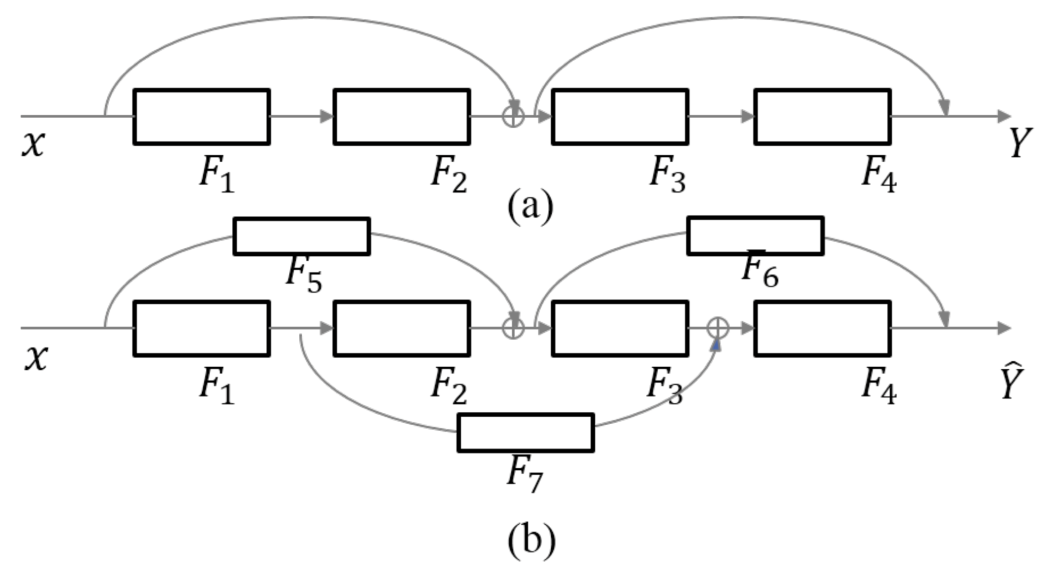
Being motivated by [35], we design a symmetric residual learning module with more skips, so that the flow of information between convolutional blocks can be further enhanced. We briefly explain the difference between symmetric residual and classical residual through an illustration. ${\{F_i\}}_{i=1}^7$ denote convolutional blocks. Figure 2a shows the classical residual module, and the output Y is calculated as,

$$Y=[F_2(F_1(x))+x]+F_4(F_3([F_2(F_1(x))+x]).$$

(4)

In the symmetric residual module (b), the output is expressed as,

$$\widehat{Y}=F_6[F_2(F_1(x))+F_5(x)]+F_4\left[F_3([F_2(F_1(x))+F_5(x)]+F_7(F_1(x)))\right].$$

(5)

It can be seen that through further linking, the final output can effectively realize the repeated use of different convolutional layer features, which greatly enhances the performance of feature extraction.

4.1.2. The Non-Local Spatial-Spectral Attention Module

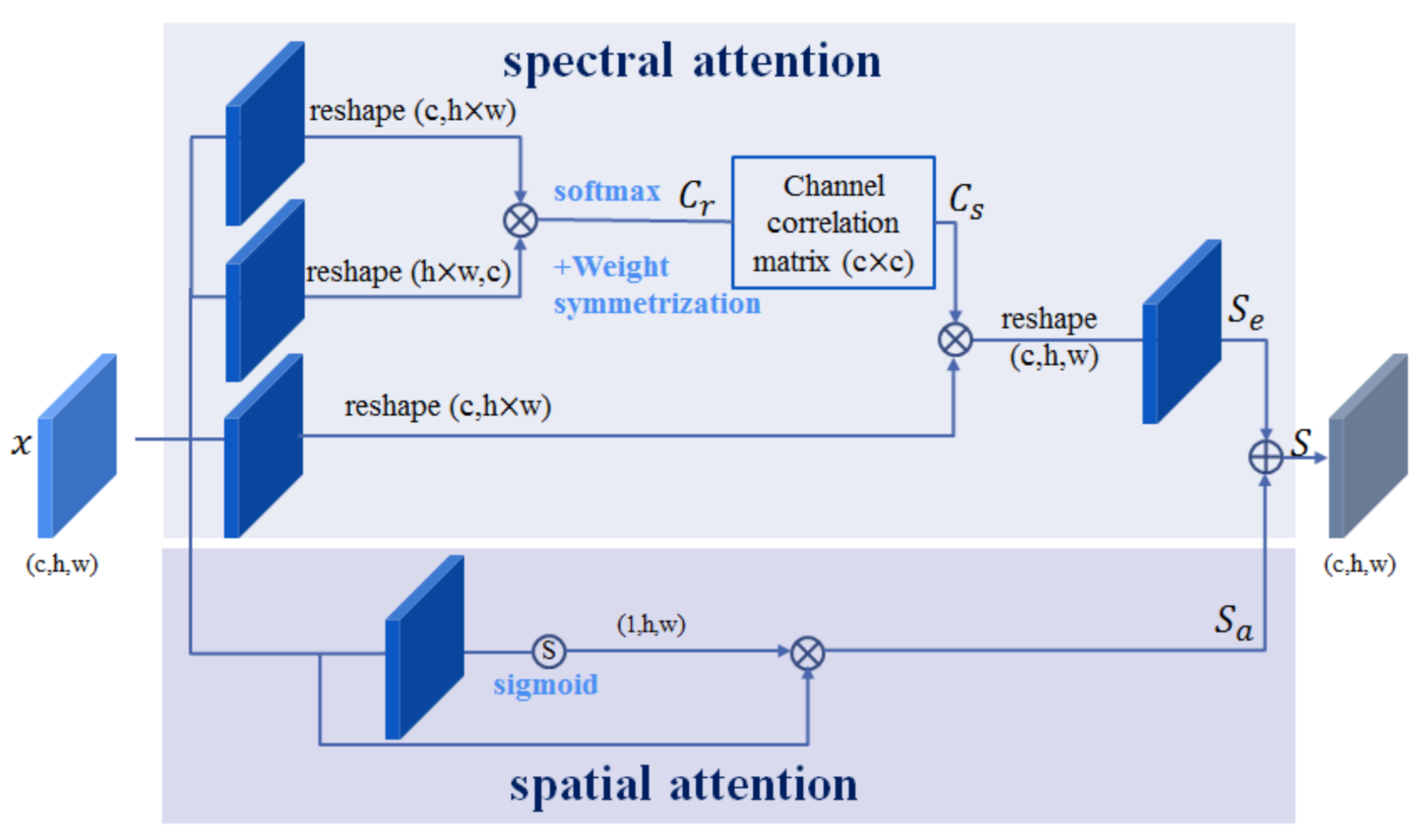
As mentioned above, HSI exhibits coupled spatial-spectral correlation. For sake of capturing this correlation, we propose a non-local spatial-spectral attention module with the spectral attention path and the spatial attention path. The spectral attention calculates the non-local correlation inter spectral channels, as shown in Figure 3. The spatial attention path focuses on the spatial correlation of hyperspectral images. The final output S is the sum of spectral attention attended feature maps $S_e$ and spatial attention attended feature maps $S_a$.

We now present the detailed processing of spectral attention path. Let $x\in R^{H\times W\times B}$ denote the input of this module. After $1\times 1$ convolution operation upon x and dimension reshaping, we can obtain two matrices with sizes $(B,H\times W)$ and $(H\times W,B)$, respectively. Subsequently, a weighted correlation matrix $C_r\in R^{B\times B}$ can be calculated after multiplying these two matrices and performing the $softmax$ operation. $C_r$ represents the global correlation between the feature maps of different channels in Equation (6). Different from the non-local processing in spatial-dimension in [33], our non-local processing occurs in the spectral dimension, and the spectral dimension B is usually much smaller than spatial dimension. Therefore, the entire non-local spectral correlation prediction does not take up a lot of calculation and memory. After this operation, we also add weight symmetrization [36] to obtain a symmetric correlation matrix $C_s$. The weight symmetrization can be briefly expressed by a linear operator [36]. Subsequently, the feature map x is subjected to $1\times 1$ convolution processing and then multiplication with $C_s$. After the succeeding $1\times 1$ convolution and reshaping operation, we can obtain the final output $Se$ of the spectral attention path. At the same time, in the spatial attention path, we use spatial attention to extract the spatial correlation of each feature map. The processing operation of the non-local spatial-spectral attention module can be mathematically formulated as:

$$\begin{array}{c}{C}_r=softmax({\varphi }_1(x)\times {\varphi }_2(x))\hfill \\ C_s=\frac{C_r+C_r^T}{2}\hfill \\ S_e=conv(C_s\times g(x))\hfill \\ S_a=x\odot sigmoid(conv(x))\hfill \\ S=S_e+S_a\hfill \end{array}$$

(6)

where $\varphi ,g$ indicates the corresponding convolution operation, × is the matrix multiplication, ⊙ is the element-wise multiplication, and $C_r^T$ represents the transposition operation of the weighted correlation matrix $C_r$. The coupled spatial-spectral correlation can be effectively represented by the incorporation of spectral attention path and spatial attention path. The ablation studies shown in Section 5 verify the effectiveness of the proposed non-local spatial-spectral attention module.

4.1.3. Loss Function

We design a compound loss function consisting of the reconstruction loss, the measurement loss, and the cosine loss to better guide the network learning. The reconstruction loss $L_{reconstruction}$ directly considers the geometric distance between hyperspectral images, and the measurement loss $L_{measurement}$ is the $L_1$ loss between the snapshot measurement y of the original HSI and the snapshot measurement $\widehat{y}$ of the network reconstructed image. The cosine loss $L_{cosine}$ is more helpful in maintaining the characteristics of the spectral signature. It determines the average cosine distance between hyperspectral pixels, treating them as vectors with the same dimension as the number of spectral bands. The mathematical formulation of the cosine loss between two hyperspectral pixels is defined as

$$l_{cosine}(i,j)=1-\cos ({\theta }_{i,j})=1-\frac{{\sum }_{b=1}^B{x}_{i,j,b}{\widehat{x}}_{i,j,b}}{\sqrt{{\sum }_{b=1}^B{x}_{i,j,b}^2}\sqrt{{\sum }_{b=1}^B{\widehat{x}}_{i,j,b}^2}},$$

(7)

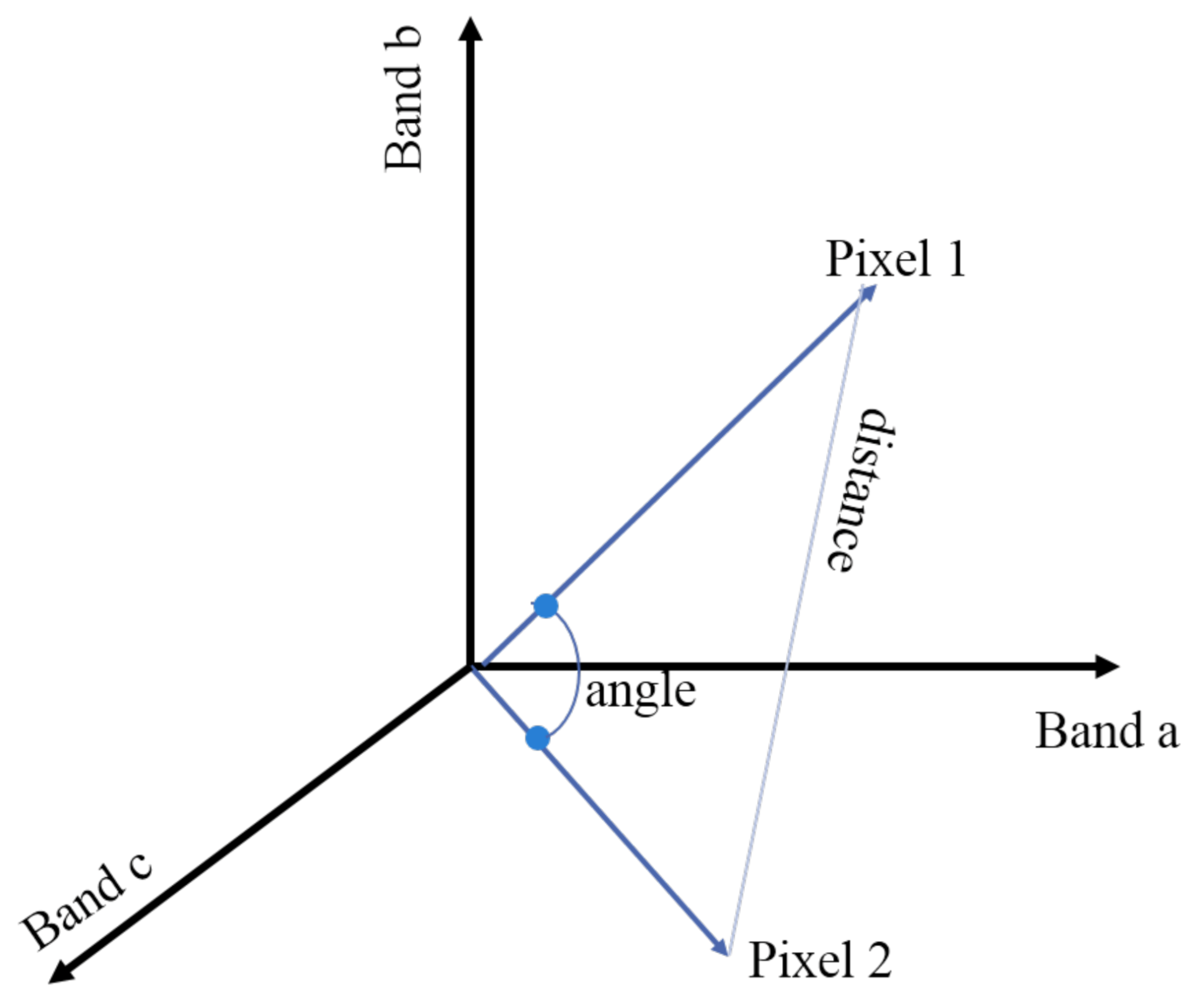
where x is the ground truth of HSI, $\widehat{x}$ is the reconstructed HSI, $x_{i,j,b}$ denotes the entry of x at spatial location $(i,j)$ and spectral band b, and $\theta$ is the spectral angle formed between reference hyperspectral pixel and reconstructed hyperspectral pixel. Figure 4 shows a concise diagram of the spectral angle and geometric distance between pixel 1 and pixel 2. The spectral cosine distance and the geometric distance are measured by cosine loss and $L_1$ loss, respectively. With the joint constraints of the distance difference and the angle difference, the reconstructed HSI can be as close as possible to the original HSI in each spectral band.

Finally, the overall compound loss function is mathematically defined as:

$$\begin{array}{c}{L}_{total}(\mathsf{\Theta })=L_{reconstruction}+{\gamma }_1{L}_{measurement}+{\gamma }_2{L}_{cosine}\hfill \\ \left\{\begin{array}{c}{L}_{reconstruction}={∥\widehat{x}-x∥}_1,\hfill \\ L_{measurement}={∥\widehat{y}-y∥}_1,\hfill \\ L_{cosine}=\frac{1}{HW}{\displaystyle \sum _{i=1}^H}{\displaystyle \sum _{j=1}^W}{l}_{cosine}(i,j),\hfill \end{array}\right.\hfill \end{array}$$

(8)

where H, W are the spatial sizes of x, ${\gamma }_1$ and ${\gamma }_2$ are the parameters that tweak the weights of each term.

5. Experiments

In this section, we conduct a series of experiments, including the comparative experiments and ablation experiments, to evaluate the performance of the proposed method. The methods to be compared with our method include several start-of-the-art methods, namely, TwIST [37], GAP-TV [38], DeSCI [18], and $\lambda$-net [26]. The first three are Prior-Driven methods, and the last is the Network-Driven method. For a comprehensive evaluation, we perform a series of comparisons on simulation and real data.

5.1. Experimental Setting

All of the experiments are performed on an NVIDIA GTX TITAN X GPU. We employ Pytorch to implement the proposed network. Our network is trained from scratch and initializes all of the convolutional layers using the default setting of the Pytorch. The Adam optimizer [39] is used to minimize the loss function and its hyper parameters are set as learning rate lr = 0.00025, betas = (0.9, 0.999), eps = ${10}^{-8}$, weight decay = 0. The batch size is 10. All of the competing methods use the code published by their authors.

We used the same data set to train the proposed network, as in [26]. The training data set of [26] contains 150 hyperspectral images with a size of $1392\times 1300\times 31$ randomly selected from the ICVL dataset, and then a spectral interpolation is used to transform their channels from the original 31 channels into 24 channels. The wavelength range of these 24 channels is from 400 nm to 700 nm, and the wavelength of each spectral band is: 398.62, 404.40, 410.57, 417.16, 424.19, 431.69, 439.70, 448.25, 457.38, 467.13, 477.54, 488.66, 500.54, 513.24, 526.8, 541.29, 556.78, 573.33, 591.02, 609.93, 630.13, 651.74, 674.83, 699.51 nm. In the process of network training, data cubes with a size of $256\times 256\times 24$ are randomly cut out from these hyperspectral data for data augmentation. Following the experimental strategy that was used in [26], the same test set was composed of 10 hyperspectral images is also used in this paper. These 10 test hyperspectral images are also selected from the ICVL dataset and their size is $256\times 256\times 24$.

5.2. Evaluation Metrics

Three quantitative image quality metrics, including PSNR, SSIM, and SAM [40,41], are used to evaluate the performance of various methods. Peak Signal to Noise Ratio (PSNR) and Structural SIMilarity (SSIM) are the first two metrics, which are widely used in the image restoration field. For hyperspectral images, we calculate the spatial fidelity of each 2D spectral band and use the average of all spectral bands as the final output. The higher the values of PSNR and SSIM, the better the performance. The last metric is Spectral Angle Mapper (SAM) [40], which is a specified metric in the hyperspectral image field. It measures the spectral fidelity between the hyperspectral pixels. Smaller SAM values indicate better reconstruction.

5.3. Ablation Studies

We conduct two ablation experiments to investigate the effectiveness of cosine loss and non-local spatial-spectral attention module. First, we test the impact of the non-local spatial-spectral attention module by removing it from the original network and evaluating the performance changes brought about by it.

Table 1. Ablation study for the non-local spatial-spectral attention module and the cosine loss. The numbers after ± denote standard deviations.

Configuration	PSNR ↑	SSIM ↑	SAM↓
without Non-local Module	34.019 (±0.141)	0.967 (±0.0020)	0.091 (±0.0005)
without Cosine Loss	34.303 ($\pm 0.138$)	0.970 ($\pm 0.0005$)	0.092 ($\pm 0.0005$)
NSSR-Net	34.764 ($\pm 0.114$)	0.972 ($\pm 0.0009$)	0.089 ($\pm 0.0005$)

shows the results of ablation studies, which are obtained as the average of three runs. Table 1 also reports the standard deviations of three quantitative metrics. It can be seen from Table 1 that the non-local spatial-spectral attention module can improve all the three metrics, which fully affirms its effectiveness. Furthermore, keeping the network architecture unchanged, we test the influence of the cosine loss term on network learning. According to the experimental results shown in Table 1, the cosine loss is conducive to improving SAM metrics of the reconstruction. Overall, the non-local spatial-spectral attention module and the compound loss term can better constrain the network learning and enhance the reconstruction performance, thus demonstrating the rationality of the NSSR-Net design.

We visualize four-channel feature maps before and after the processing of this module in Figure 5 to further analyze the role of the non-local spatial-spectral attention module. It can be seen that the feature maps after the processing of the non-local spatial-spectral attention module can have significantly more informative structures, which demonstrates the advantage of taking the spatial-spectral joint correlation in the reconstruction network.

5.4. Simulation Data Results

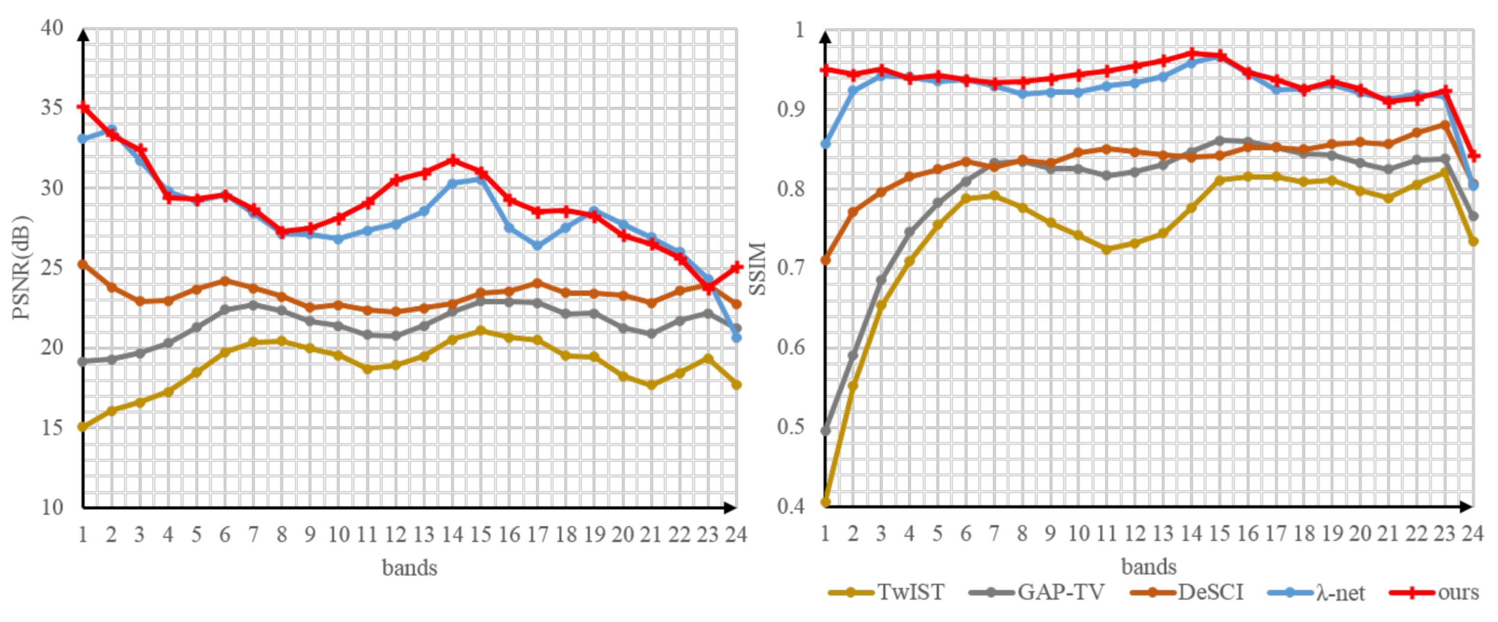
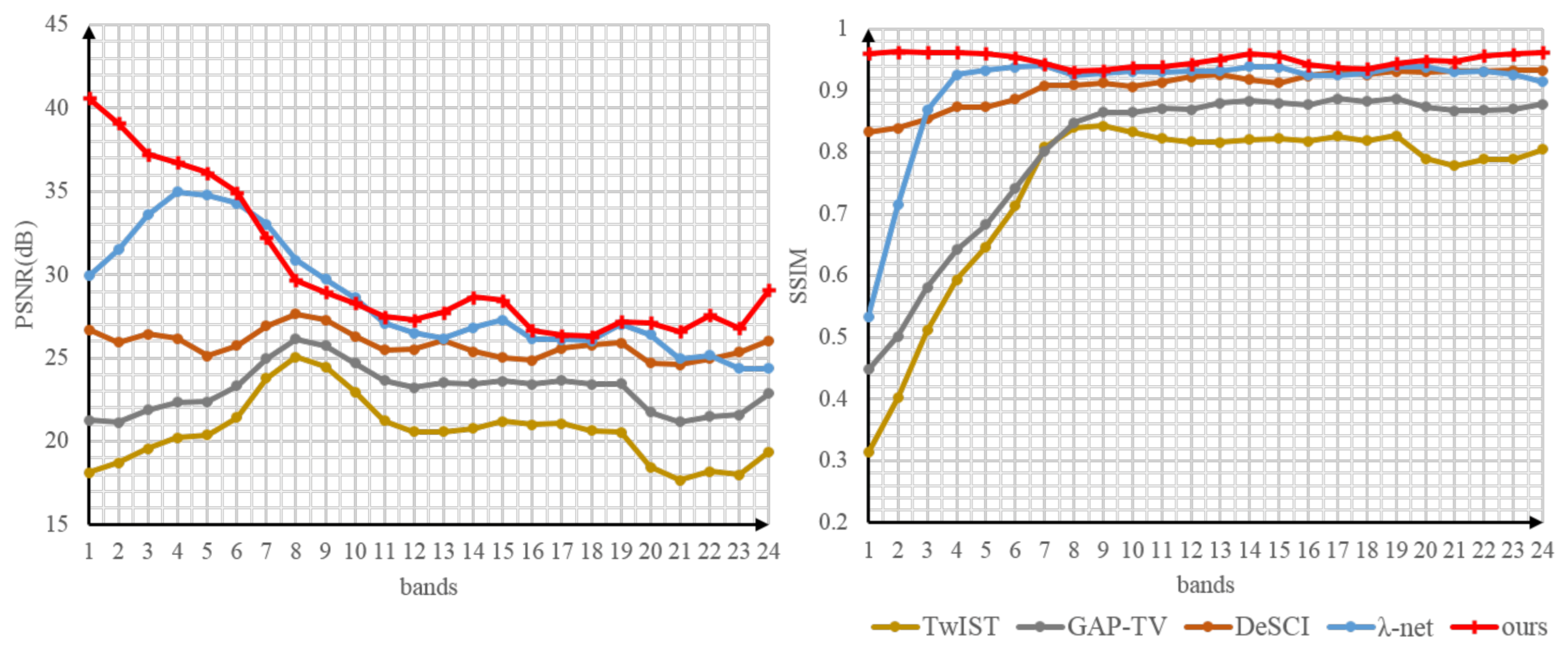
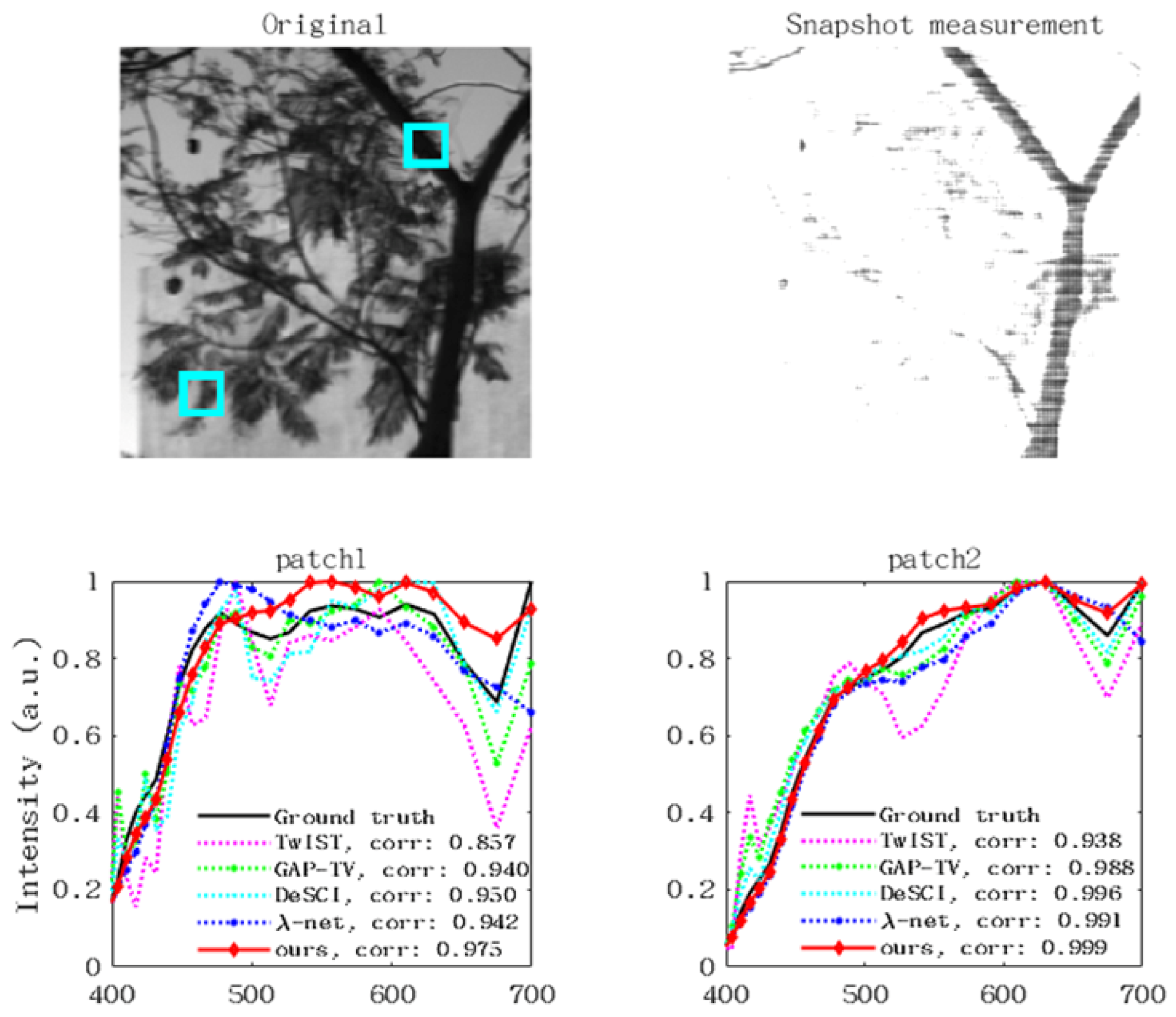
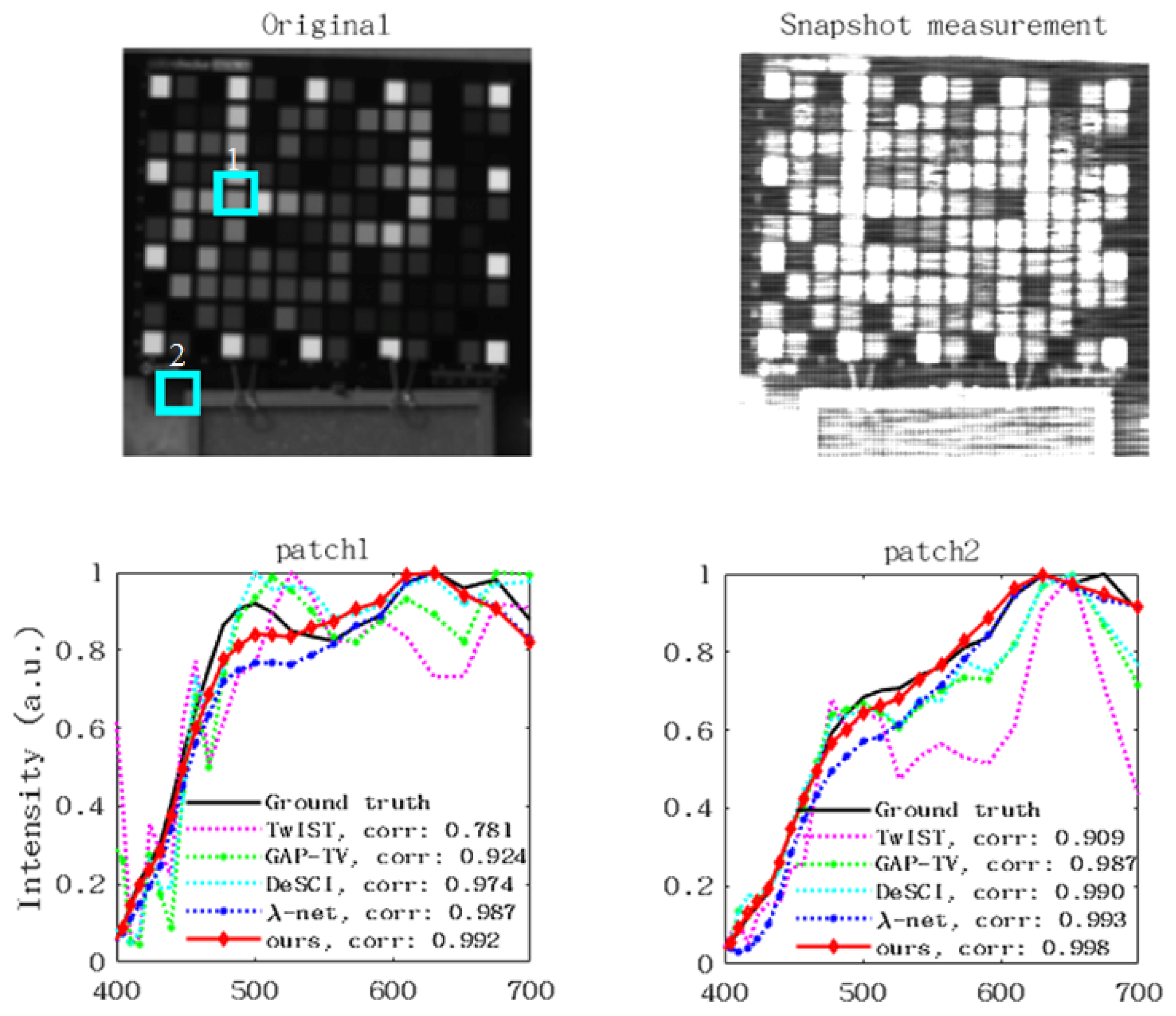
In this Simulation case, we use the same coded masks as in [26], which are from the real CASSI system and used to generate snapshot measurements of the test HSIs.

Table 2. Quantitative result comparison on 10 test images from the ICVL dataset.

Methods	Metrics	Scene 1	Scene 2	Scene 3	Scene 4	Scene 5	Scene 6	Scene 7	Scene 8	Scene 9	Scene 10	Average
TwIST	PSNR	25.621	18.413	21.750	21.240	23.784	20.579	24.232	20.202	27.014	18.921	22.140
	SSIM	0.856	0.826	0.826	0.828	0.799	0.744	0.870	0.784	0.888	0.747	0.817
	SAM	0.160	0.175	0.192	0.197	0.235	0.335	0.173	0.199	0.226	0.241	0.213
GAP-TV	PSNR	30.666	22.410	23.499	22.273	26.985	23.090	24.859	22.913	29.105	21.502	24.730
	SSIM	0.892	0.869	0.863	0.829	0.792	0.802	0.877	0.841	0.912	0.796	0.847
	SAM	0.207	0.185	0.302	0.184	0.330	0.334	0.166	0.186	0.225	0.213	0.233
DeSCI	PSNR	31.147	26.443	24.741	29.251	29.372	25.814	28.401	24.424	34.411	23.331	27.732
	SSIM	0.937	0.947	0.898	0.949	0.907	0.906	0.921	0.872	0.971	0.834	0.914
	SAM	0.168	0.081	0.263	0.105	0.229	0.262	0.148	0.186	0.175	0.190	0.181
$\lambda$-Net	PSNR	36.109	32.054	33.341	29.598	35.403	28.573	35.219	32.355	33.418	28.204	32.427
	SSIM	0.949	0.975	0.974	0.937	0.942	0.902	0.969	0.951	0.916	0.924	0.944
	SAM	0.098	0.043	0.091	0.100	0.129	0.205	0.071	0.099	0.200	0.113	0.115
NSSR-Net (ours)	PSNR	40.044	36.557	34.632	29.225	38.474	30.002	38.298	33.886	37.217	28.924	34.726
	SSIM	0.988	0.989	0.972	0.953	0.984	0.944	0.985	0.966	0.987	0.937	0.971
	SAM	0.055	0.027	0.073	0.114	0.081	0.198	0.046	0.075	0.123	0.107	0.090

shows the PSNR, SSIM, and SAM values of five methods on 10 test images. According to the quantitative metrics in Table 2, our method has the best average PSNR, SSIM, and SAM values. Figure 6 and Figure 7 show the plots of PSNR and SSIM values of two scenes as a function of the number of spectral bands. The PSNR and SSIM plots of our method lie basically at the top, and our method does not show a sudden drop in reconstruction quality at certain spectral bands. Figure 8 and Figure 9 provide the snapshot measurements that correspond to the two scenes, as well as the reconstructed spectral signatures in the patches that are indicated by the rectangles. The correlation coefficients that are presented in the legend demonstrate that our method can reconstruct more accurate spectral signatures when compared with the other methods. Figure 10 and Figure 11 visualize the reconstructed spectral bands of two scenes. We can see that our algorithm can reconstruct clear structures and fine details. We also compare the reconstructed spectral signatures of different methods. Our method can better maintain the fidelity of the spectral signatures than the competitive methods.

5.5. Real Data Results

The real data used in our experiments is the Bird data captured by the hyperspectral imaging camera (The Bird data is downloaded from [18]’s Github homepage https://github.com/liuyang12/DeSCI.2019, accessed on 1 February 2020). Because of the complexity of hardware in the real imaging system, the obtained snapshot measurement of Bird hyperspectral data is troubled by noise, which makes reconstruction more difficult. The spatial size of the original real Bird data is $1021\times 703$ and contains 24 spectral bands. We cropped a $512\times 512$ sub-image for performance evaluation and comparison due to the limitation of computational resource of hardware.

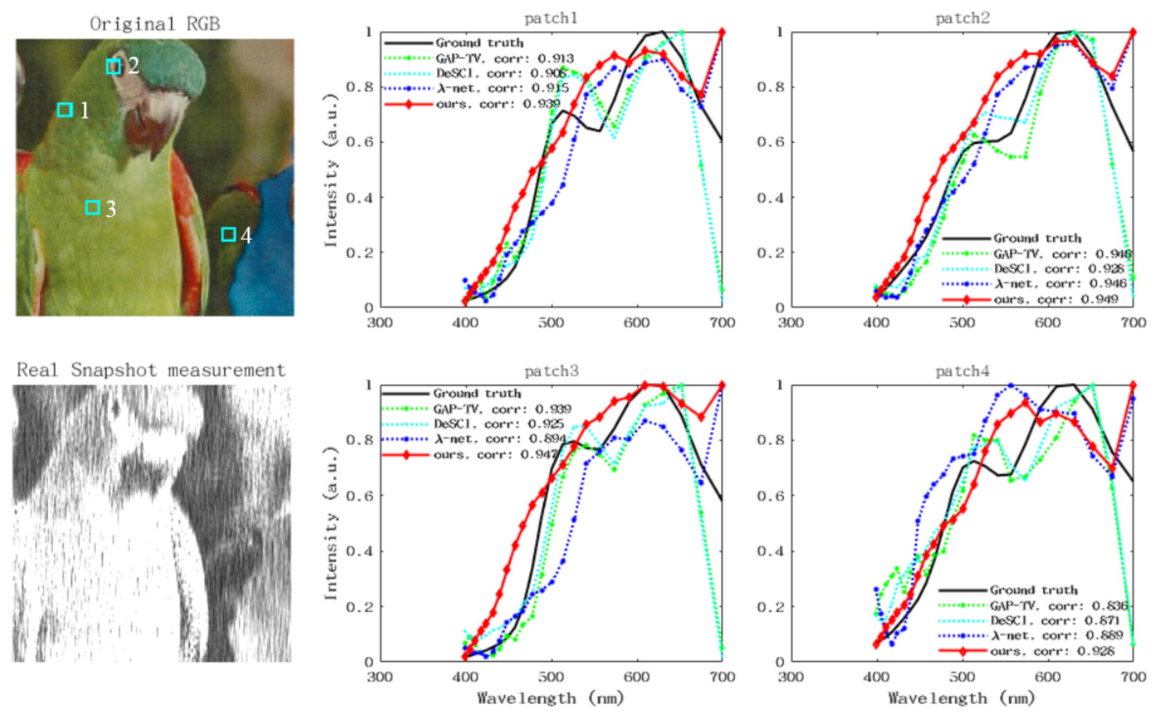
Figure 12 shows four reconstructed spectral bands of Bird data. The reconstruction of GAP-TV still contains a lot of noise when compared with the Ground-truth, as can be seen from Figure 12. Although DeSCI can smooth out the noise, its reconstructed images lack texture details. Regarding the last spectral band (699.51 nm), only $\lambda$-net and our method can reconstruct the main structures of this spectral band. $\lambda$-net and our method have the similar visual quality. In terms of quantitative metric, our method has the best PSNR and SSIM values. Figure 13 shows the spectral correlation between the reconstruction results of each method and the ground truth. It can be seen that our method has the superiority of maintaining the fidelity of spectral signatures over the other methods.

5.6. Time Complexity Analysis

In addition to the quantitative indicators of reconstruction quality, it is also necessary to analyze the time complexity of the reconstruction methods. Therefore, we also compare the running time (in seconds) that is consumed by each method in reconstructing $256\times 256\times 24$ hyperspectral images. TwIST, GAP-TV, and DeSCI run on the CPU, while DeSCI and the proposed method run on the GPU.

Table 3. The average run time for the reconstruction of a $256\times 256\times 24$ hyperspectral image.

Methods	TwIST	GAP-TV	DeSCI	$\mathit{\lambda }$-Net	NSSR-Net
Times (s)	70.96	25.8	3594.5	4.28	1.19

shows the running time results of each algorithm. It can be seen that the reconstruction speed of the Network-Driven method is faster than that of the Prior-Driven methods, because the Network-Driven methods do not require iterative optimization. Because of the two stages of cascaded reconstruction in $\lambda$-Net, its reconstruction process consumes more time than our method.

6. Conclusions

In this paper, we propose a novel network for HSI snapshot reconstruction from a single measurement. First, we design the symmetric residual module to integrate the fusion of local features. We propose a non-local spatial-spectral attention module to fully utilize this prior structures to further consider the joint correlation of the spatial and spectral of the HSI. Besides, the compound loss is designed to guide the network focus more on detail reconstruction. The experiment results on both simulation and real data have verified that our method has good performance, while maintaining a fast reconstruction time.

References

1. Chakrabarti, A.; Zickler, T. Statistics of real-world hyperspectral images. In Proceedings of the IEEE Conference on Computer Vision and Pattern Recognition, Colorado Springs, CO, USA, 20–25 June 2011; pp. 193–200. [Google Scholar]
2. Tu, B.; Zhou, C.; Liao, X.; Zhang, G.; Peng, Y. Spectral-Spatial Hyperspectral Classification via Structural-Kernel Collaborative Representation. IEEE Geosci. Remote Sens. Lett. 2020, 18, 861–865. [Google Scholar] [CrossRef]
3. Ojha, L.; Wilhelm, M.B.; Murchie, S.L.; McEwen, A.S.; Wray, J.J.; Hanley, J.; Massé, M.; Chojnacki, M. Spectral evidence for hydrated salts in recurring slope lineae on Mars. Nat. Geosci. 2015, 8, 829–832. [Google Scholar]
4. Cao, X.; Zhou, F.; Xu, L.; Meng, D.; Xu, Z.; Paisley, J. Hyperspectral image classification with markov random fields and a convolutional neural network. IEEE Trans. Image Process. 2018, 27, 2354–2367. [Google Scholar] [CrossRef] [PubMed] [Green Version]
5. Fauvel, M. Advances in spectral-spatial classification of hyperspectral images. Proc. IEEE 2012, 101, 652–675. [Google Scholar] [CrossRef] [Green Version]
6. Mouroulis, P.; Green, R.O.; Chrien, T.G. Design of pushbroom imaging spectrometers for optimum recovery of spectroscopic and spatial information. Appl. Opt. 2000, 39, 2210–2220. [Google Scholar] [CrossRef] [Green Version]
7. Wehr, A.; Lohr, U. Airborne laser scanning-an introduction and overview. ISPRS J. Photogramm. Remote Sens. 1999, 54, 68–82. [Google Scholar] [CrossRef]
8. Shogenji, R.; Kitamura, Y.; Yamada, K. Multispectral imaging using compact compound optics. Opt. Express 2004, 12, 1643–1655. [Google Scholar] [CrossRef]
9. Arce, G.; Brady, D.; Carin, L.; Arguello, H.; Kittle, D. Compressive coded aperture spectral imaging: An introduction. IEEE Signal Process. Mag. 2014, 31, 105–115. [Google Scholar] [CrossRef]
10. Wagadarikar, A.; John, R.; Willett, R.; Brady, D. Single disperser design for coded aperture snapshot spectral imaging. OSA Appl. Opt. 2008, 47, 44–51. [Google Scholar] [CrossRef] [Green Version]
11. Donoho, D.L. Compressed sensing. IEEE Trans. Inf. Theory 2006, 52, 1289–1306. [Google Scholar] [CrossRef]
12. Wang, Y.; Yang, J.; Yin, W.; Zhang, Y. A new alternating minimization algorithm for total variation image reconstruction. SIAM J. Imaging Sci. 2008, 1, 248–272. [Google Scholar] [CrossRef]
13. Buades, A.; Coll, B.; Morel, J.-M. A non-local algorithm for image denoising. IEEE Conf. Comput. Vis. Pattern Recognit. 2005, 2, 60–65. [Google Scholar]
14. Elad, M.; Aharon, M. Image denoising via sparse and redundant representations over learned dictionaries. IEEE Trans. Image Process. 2006, 15, 3736–3745. [Google Scholar] [CrossRef]
15. Lecun, Y.; Bengio, Y.; Hinton, G. Deep learning. Nature 2015, 521, 436–444. [Google Scholar] [CrossRef]
16. Kittle, D.; Choi, K.; Wagadarikar, A.; Brady, D.J. Multiframe image estimation for coded aperture snapshot spectral imagers. Appl. Opt. 2010, 49, 6824–6833. [Google Scholar] [CrossRef]
17. Wang, L.; Xiong, Z.; Shi, G.; Wu, F.; Zeng, W. Adaptive nonlocal sparse representation for dual-camera compressive hyperspectral imaging. IEEE Trans. Pattern Anal. Mach. Intell. 2017, 39, 2104–2111. [Google Scholar] [CrossRef]
18. Yuan, X. Generalized alternating projection based total variation minimization for compressive sensing. IEEE Trans. Pattern Anal. Mach. Intell. 2019, 41, 2990–3006. [Google Scholar]
19. Blumensath, T.; Davies, M.E. Iterative hard thresholding for compressed sensing. Appl. Comput. Harmon. Anal. 2009, 27, 265–274. [Google Scholar] [CrossRef] [Green Version]
20. Sun, Y.; Chen, J.; Liu, Q.; Liu, B.; Guo, G. Dual-Path Attention Network for Compressed Sensing Image Reconstruction. IEEE Trans. Image Process. 2020, 29, 9482–9495. [Google Scholar] [CrossRef]
21. Sun, Y.; Yang, Y.; Liu, Q.; Chen, J.; Yuan, X.-T.; Guo, G. Learning Non-Locally Regularized Compressed Sensing Network With Half-Quadratic Splitting. IEEE Trans. Multimed. 2020, 22, 3236–3248. [Google Scholar] [CrossRef]
22. Xiong, Z.; Shi, Z.; Li, H.; Wang, L.; Liu, D.; Wu, F. Hscnn: Cnn-based hyperspectral image recovery from spectrally undersampled projections. In Proceedings of the IEEE International Conference on Computer Vision (ICCV), Venice, Italy, 22–29 October 2017; pp. 518–525. [Google Scholar]
23. Choi, I.; Jeon, D.S.; Nam, G.; Gutierrez, D.; Kim, M.H. High-quality hyperspectral reconstruction using a spectral prior. ACM Trans. Graph. 2017, 36, 218. [Google Scholar] [CrossRef] [Green Version]
24. Wang, L.; Sun, C.; Zhang, M.; Fu, Y.; Huang, H. DNU: Deep Non-Local Unrolling for Computational Spectral Imaging. In Proceedings of the IEEE/CVF Conference on Computer Vision and Pattern Recognition (CVPR), Seattle, WA, USA, 13–19 June 2020; pp. 1658–1668. [Google Scholar]
25. Zheng, S.; Liu, Y.; Meng, Z.; Qiao, M.; Tong, Z.; Yang, X.; Han, S.; Yuan, X. Deep plug-and-play priors for spectral snapshot compressive imaging. Photonics Res. 2021, 9, B18–B29. [Google Scholar] [CrossRef]
26. Miao, X.; Yuan, X.; Pu, Y. lambda-net: Reconstruct Hyperspectral Images from a Snapshot Measurement. In Proceedings of the IEEE/CVF International Conference on Computer Vision (ICCV), Seoul, Korea, 27 October–2 November 2019; pp. 4058–4068. [Google Scholar]
27. Vaswani, A.; Shazeer, N.; Parmar, N. FAttention is all you need. In Proceedings of the Advances in Neural Information Processing Systems, Long Beach, CA, USA, 4–9 December 2017; pp. 5998–6008. [Google Scholar]
28. Sun, H.; Zheng, X.; Lu, X.; Wu, S. Spectral–Spatial Attention Network for Hyperspectral Image Classification. IEEE Trans. Geosci. Remote Sens. 2020, 58, 3232–3245. [Google Scholar] [CrossRef]
29. Sellami, A.; Abbes, A.B.; Barra, V. Fused 3-D spectral-spatial deep neural networks and spectral clustering for hyperspectral image classification. Pattern Recognit. Lett. 2020, 138, 594–600. [Google Scholar] [CrossRef]
30. Sellami, A.; Abbes, A.B.; Barra, V. Hyperspectral Image Classification Based on 3-D Octave Convolution With Spatial–Spectral Attention Network. IEEE Trans. Geosci. Remote Sens. 2021, 59, 2430–2447. [Google Scholar]
31. Zhang, X.; Huang, W.; Wang, Q.; Li, X. SSR-NET: Spatial-Spectral Reconstruction Network for Hyperspectral and Multispectral Image Fusion. IEEE Trans. Geosci. Remote Sens. 2020, 1–13. [Google Scholar] [CrossRef]
32. Meng, Z.; Ma, J.; Yuan, X. End-to-end low cost compressive spectral imaging with spatial-spectral self-attention. In Proceedings of the European Conference on Computer Vision, Glasgow, UK, 23–28 August 2020; pp. 187–204. [Google Scholar]
33. Wang, X.; Girshick, R.; Gupta, A.; He, K. Non-local Neural Networks. In Proceedings of the IEEE Conference on Computer Vision and Pattern Recognition (CVPR), Salt Lake City, UT, USA, 18–23 June 2018; pp. 7794–7803. [Google Scholar]
34. He, K.; Zhang, X.; Ren, S.; Sun, J. Deep Residual Learning for Image Recognition. In Proceedings of the IEEE Conference on Computer Vision and Pattern Recognition (CVPR), Las Vegas, NV, USA, 27–30 June 2016; pp. 770–778. [Google Scholar]
35. Liu, X.; Suganuma, M.; Sun, Z.; Okatani, T. Dual Residual Networks Leveraging the Potential of Paired Operations for Image Restoration. In Proceedings of the IEEE Conference on Computer Vision and Pattern Recognition (CVPR), Long Beach, CA, USA, 15–20 June 2019; pp. 7000–7009. [Google Scholar]
36. Hu, X.S.; Zagoruyko, S.; Komodakis, N. Exploring Weight Symmetry in Deep Neural Networks. arXiv 2018, arXiv:1812.11027. [Google Scholar] [CrossRef] [Green Version]
37. Bioucas-Dias, J.M.; Figueiredo, M.A. A new twist: Two-step iterative shrinkage/thresholding algorithms for image restoration. IEEE Trans. Image Process. 2007, 16, 2992–3004. [Google Scholar] [CrossRef] [Green Version]
38. Liu, Y.; Yuan, X.; Suo, J.; Brady, D.; Dai, Q. Rank minimization for snapshot compressive imaging. IEEE Int. Conf. Image Process. 2016, 16, 2539–2543. [Google Scholar] [CrossRef] [Green Version]
39. Diederik, P.K.; Jimmy, B. Adam: A method for stochastic optimization. In Proceedings of the 33rd International Conference on Learning Representations, San Diego, CA, USA, 7–9 May 2015; pp. 1–15. [Google Scholar]
40. Liu, X.; Yang, C. A Kernel Spectral Angle Mapper algorithm for remote sensing image classification. In Proceedings of the International Congress on Image and Signal Processing (CISP), Beijing, China, 14–16 July 2013; pp. 814–818. [Google Scholar]
41. Wang, Z.; Bovik, A.C.; Sheikh, H.R.; Simoncelli, E.P. Image quality assessment: From error visibility to structural similarity. IEEE Trans. Image Process. 2004, 13, 600–612. [Google Scholar] [CrossRef] [Green Version]
Figure 1. The overall framework of the proposed method. It consists of the training stage and test stage. The reconstruction of test image can be obtained by just feeding the CASSI measurement into the well-trained network.
Remotesensing 13 01812 g001
Figure 2. A simple explanation of the symmetric residual module. (a) is the original residual block, (b) is a symmetric residual module with seven convolutional blocks.
Remotesensing 13 01812 g002
Figure 3. The Non-local Spatial-spectral Attention Module, consisting of the spectral attention and spatial attention.
Remotesensing 13 01812 g003
Figure 4. A diagram of the spectral angle and geometric distance between pixel 1 and pixel 2 of a HSI with three bands.
Remotesensing 13 01812 g004
Figure 5. Visualization of feature maps. The upper column is feature maps before the non-local spatial-spectral attention module, and the lower is feature maps after processing by this module.
Remotesensing 13 01812 g005
Figure 6. The plot of PSNR and SSIM values of scene 10 as a function of the number of spectral bands.
Remotesensing 13 01812 g006
Figure 7. The plot of PSNR and SSIM values of scene 6 as a function of the number of spectral bands.
Remotesensing 13 01812 g007
Figure 8. The snapshot measurement of scene 10 and the reconstructed spectral signatures. The first row shows one spectral bands of the scene 10 and its snapshot measurement. The second row show the reconstructed spectral signatures of the two patches indicated by the rectangles. The correlation coefficients are also shown in the legend to quantitatively compare the accuracy of the spectral signatures that were reconstructed by the five methods.
Remotesensing 13 01812 g008
Figure 9. The snapshot measurement of scene 6 and the reconstructed spectral signatures. The first row shows one spectral bands of the scene 6 and its snapshot measurement. The second row show the reconstructed spectral signatures of the two patches indicated by the rectangles. The correlation coefficients are also shown in the legend to quantitatively compare the accuracy of the spectral signatures reconstructed by the five methods.
Remotesensing 13 01812 g009
Figure 10. The visualization of four spectral bands of scene 10 (wavelength: 477.54 nm, 526.8 nm, 630.13 nm and 699.51 nm) reconstructed by five methods. From the left column to the rightmost column correspond to Ground truth, TwIST (PSNR 18.921/SSIM 0.747), GAP-TV (21.502/0.796), DeSCI (23.331/0.834), λ -net (28.204/0.924) and ours (28.924/0.937).
Remotesensing 13 01812 g010
Figure 11. The visualization of four spectral bands of scene 6 (wavelength: 477.54 nm, 526.8 nm, 630.13 nm and 699.51 nm) reconstructed by five methods. From the left column to the rightmost column correspond to Ground truth, TwIST (PSNR 20.579/SSIM 0.744), GAP-TV (23.090/0.802), DeSCI(25.814/0.906), λ -net (28.573/0.902), and ours (30.002/0.944).
Remotesensing 13 01812 g011
Figure 12. Real data results: Four reconstructed spectral bands (wavelengths from top to bottom are 477.54 nm, 541.29 nm, 591.02 nm, and 699.51 nm). On the far left is the ground truth of Bird real data, and to the right are the reconstruction results of GAP-TV (22.540/0.754), DeSCI (25.036/0.777), λ -net (24.882/0.832), and ours (25.389/0.839). The numbers in the brackets are the PSNR and SSIM values corresponding to each method.
Remotesensing 13 01812 g012
Figure 13. Real data results: the reconstructed spectral signatures of the Bird hyperspectral data captured by the real CASSI system. The correlation coefficients of the reconstructed spectral signatures and the ground-truth are shown in the legends.
Remotesensing 13 01812 g013