Abstract
Non-linear behavioral links with atmospheric teleconnections were identified between the Indian Ocean Dipole (IOD) mode and seasonal precipitation over East Asia (EA) using statistical models. The analysis showed that the lower the lag time, the higher the correlation; more than a two-fold correlation for non-linear regression with a kernel density estimator than for the linear regression method. When the IOD peaked, a pattern of significant reductions in seasonal precipitation during the negative IOD period occurred throughout the Korean Peninsula (KP). The occurrence of the positive IOD was in line with the El Niño phenomenon and generated greater seasonal precipitation than only the positive IOD, which takes place from March to May. This change occurred more in the cold tongue El Niño than the warm pool El Niño, inducing much higher spring precipitation throughout the KP. When negative IODs and La Niña coincided, there was slightly greater precipitation from March to May compared to the sole occurrence of negative IODs. In positive (negative) IOD years, there was anti-cyclonic (cyclonic) circulation in the South China Sea (SCS), helping to transport moisture to EA. The composite precipitation anomalies in the positive (negative) IOD years show above (below) normal precipitation in southern China. In contrast, other parts of the EA experienced drier (humid) signals than normal years. In positive IOD years, the anti-cyclonic circulation strength of the Bay of Bengal and the SCS continued until autumn and spring of the following year. This shows possible remote connections between climate events related to the tropical Indian Ocean and variations in precipitation over EA.
1. Introduction
The frequency and intensity of extreme climate events have gradually increased; this has been attributed to rising global temperatures [1,2,3]. Seasonal variations in regional water resource availability are also closely linked to the characteristic changes in global climate [2,4,5,6,7]. These trends have significant implications for the efficient prediction and management of available water resources. It is increasingly important to understand the relationship between extreme climatic events and the seasonal variability of water resources using hydro-meteorological variables.
Long-term hydro-meteorological changes are highly correlated with large-scale atmospheric teleconnections that predict the behavior of non-linear climate systems using ocean-related climate indices, such as the El Niño–Southern Oscillation (ENSO) and the Indian Ocean Dipole (IOD) mode [8,9,10,11,12]. Many studies on ENSO and the IOD report the shared understanding that these systems are major sources of large-scale atmospheric environmental changes. These systems are also closely correlated with seasonal variations, such as precipitation and streamflow within local patterns of hydro-meteorological change [10,11,12,13,14,15].
The IOD mode defined by Saji et al. [10] is characterized by extreme rainfall and wet conditions in the East African region during positive IOD (p-IOD) years. During negative IOD (n-IOD) years, wet conditions typically occur in the western part of the Indian Ocean and Indonesia; this is directly impacting East Africa, triggering dry conditions. Several studies have argued that the IOD phenomenon currently precedes ENSO events evidenced by the rise in sea surface temperature (SST), leading the latter by three to six months [16,17]. However, correlation analyses between SST anomalies of ENSO and IOD in the tropical ocean region indicates that the IOD is a phenomenon that occurs independently of ENSO, and is an internal mode within the Indian Ocean region. The results from past research also demonstrate that the Indian Ocean SST is experiencing changes to its trends over time, affecting the cycle, intensity, and genesis of the IOD mode [10,18,19,20,21].
A previous study on the potential mechanism of IOD patterns over the East Asian (EA) region presented the Bonin high formation mechanism during August for the deep ridge near Japan [22]. This theory was based on the hypothesis that an equivalent-barotropic ridge near Japan was formed because of the upper troposphere (Silk Road pattern). Furthermore, Guan and Yamagata [23] suggested that the IOD event was closely related to teleconnections around Japan, Korea, and the northeastern part of China during the sweltering and dry summer of 1994. They determined that the monsoon–desert mechanism [24], producing dry conditions over the EA region, connects a Rossby wave source with IOD-induced heating around the Bay of Bengal. The upper troposphere propagates northeastward from southern China, and the Rossby wave pattern influences precipitation changes over EA. Zhang et al. [25] examined the effects of the IOD on summer precipitation over eastern China. They found that IOD forcing in the preceding autumn has a pronounced, albeit delayed, influence on the precipitation in the following summer, particularly over the Yangtze-Huaihe River Valley. Weng et al. [26] discovered a possible link between the Indian Ocean SSTA pattern and summer precipitation in China by anomalous mid- and low-level tropospheric circulations. Cai et al. [27] identified the IOD impact on Australian winter rainfall using the Rossby wave train.
IOD and ENSO patterns are considered the main causes of large-scale atmospheric change, leading to significant changes in the hydro-meteorological patterns of several EA countries [12,22,23,28,29,30]. Recent studies have suggested that global surface temperature rise may have to slow down due to significant heat transfer from the Pacific to Indian Oceans via the Indonesian Throughflow [31,32,33]. Studies on Indo-Pacific thermocouples are required to improve the current understanding of climatic variability and quantitatively diagnose such variability at a regional scale. Existing quantitative studies on the characteristics of the IOD and ENSO phenomena, relating to Korean watersheds and their regional assessments, are relatively inadequate. This study analyzed the influence of long-term precipitation variability in the EA region by examining p-IOD and n-IOD events [10]. The classification of IOD events in accordance with the patterns of p-IOD and n-IOD events was also analyzed, and the analysis of the evolution patterns of the IOD was based on the approach of Saji and Yamagata [20]. This study addresses three specific objectives: (1) to analyze the significant changes in large-scale pattern and long-term precipitation variability in the EA, and in the KP region sub-watershed using ocean-related, abnormal climate phenomena, in accordance with the IOD mode index; (2) to investigate linkages between atmospheric teleconnections and possible mechanisms between different phases of the IOD and seasonal precipitation over the KP using statistical methods; and (3) to carry out a diagnostic study on the non-stationarity and possibility of seasonal precipitation prediction, using climate indices during significant IOD and ENSO seasons over the KP.
2. Materials and Methods
2.1. Data
SST data obtained from the National Center for Environmental Prediction and the National Center for Atmospheric Research (NCEP-NCAR) reanalysis v2 were used to classify the IOD events in the Tropical Indian Ocean (TIO). IOD Mode Index (DMI) data were obtained from the Japan Agency for Marine-Earth Science and Technology (JAMSTEC) and the Hadley Centre Sea Ice and Sea Surface Temperature dataset. The DMI is defined as the SST anomaly difference between the western (50°E–70°E, 10°S–10°N) and southeastern (90°E–110°E, 10°S–equator) regions of the TIO region [10]. The DMI calculated by the Asia-Pacific Economic Cooperation Climate Center (APCC), Busan, South Korea, was used; this utilizes monthly SST from the National Oceanic and Atmospheric Administration (NOAA) Extended Reconstructed Sea Surface Temperature (ERSST) v4 in the TIO region. The Global Precipitation Climatology Center (GPCC) monthly precipitation, which has a regular grid with a spatial resolution of latitude by longitude from Deutscher Wetterdienst in Germany was used to diagnose precipitation variability and its long-term changes in the EA region. In addition, spatially averaged daily precipitation data provided by the Water Resources Management Information System (WAMIS) were used to undertake a detailed examination of the regional impact in five major Korean river basins in the KP (Figure 1). The average precipitation was calculated using the Thiessen polygon network from 125 precipitation gauge stations for 117 sub-watersheds within these five major river basins foMIr 1966–2016. For the composite analysis, monthly vector wind anomalies at 850 hPa were used; these were obtained from the NCEP-NCAR. Student’s t-test was used for statistical significance testing for composite analysis.
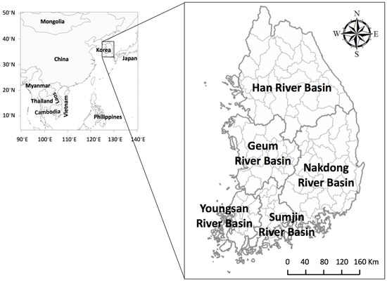
Figure 1.
Map of the East Asia region, including the location of the five major river basins of the Korean Peninsula.
2.2. Classification of IOD Events
This study used the methodology proposed by Saji and Yamagata [20] to classify positive and negative IOD events in the TIO region. The process included data pre-processing and exclusion of data that did not meet the following criteria:
- (1)
- Pre-processing of data: SST anomalies in the Western Indian Ocean (10°S–10°N, 60°–80°E) and eastern Indian Ocean (10°S–0°, 90°–110°E), and zonal wind anomalies over the equator (, area-averaged wind anomaly over 5°S–5°N, 70°–90°E), were first detrended. A three-month running mean was then applied once over the three time-series datasets to reduce the impact of intra-seasonal fluctuations;
- (2)
- Identifying criteria: The DMI and needed to exceed 0.5 in amplitude for at least three months. In addition, the SSTA in the west and east Indian Ocean have opposite signs, and the magnitude should exceed 0.5 for at least three months.
Figure 2 shows the DMI region in the Indian Ocean and the normalized anomaly time series for the DMI between the Hadley Centre Sea Ice and the Sea Surface Temperature dataset (HadISST) by the NOAA Climate Prediction Center (CPC), and the method proposed by Saji et al. [10]. Two time-series datasets were compared using a similar method; the 13 strongest p-IOD, and the 15 strongest n-IOD years were classified based on the HadISST data from 1956 to 2018.
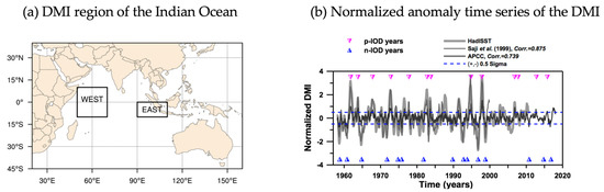
Figure 2.
The dipole mode index (DMI) region in the Indian Ocean and normalized anomaly time series for DMI. (a) DMI region in the Indian Ocean, (b) normalized anomaly time series of the DMI. In the panel of the (b), the light gray, dark gray, and solid black lines indicate calculated DMI indices by HadISST, Saji et al. [10] and APEC Climate Center (APCC), respectively. “corr” indicates the correlation coefficient.
2.3. Singular Spectrum Analysis
Singular spectrum analysis (SSA) is a non-parametric spectral estimation method that reduces dispersion by changing the coordinates in time series through techniques derived from principal component analysis (PCA); this enables the extraction of information from noisy time series. By removing the non-harmonic components from the original time series data, the long-term frequency and trend may easily be understood [34]. SSA embeds the data of a time series in a vector space of dimension , and applies the empirical orthogonal function (EOF) method. This enables the projection of original data in the orthogonal functions EOF 1 and EOF 2. By composing the axes using these EOFs, the trend, cycle, and tendency of total variance in the data, are more clearly apparent.
To separate the non-harmonic components, the size of the eigenvalues was defined by an orthogonal process. The orthogonal function was calculated between and ; these are the orthogonal coefficients of the principal component (PC1) and PC2 time series that correspond with the harmonic components in the original coordinates, X and Y. Finally, it was converted to the reconstruction component (RC) as and . The estimation forecasting model may be configured to reflect specific characteristics such as frequency and trend in the original data. By using Equation (1) to reconstruct the data, the original data may be replaced with a new time series with a constant frequency and less noise:
where is an orthogonal coefficient; is the empirical orthogonal function (); indicates a dimension; and is the sampling rate. Additional detailed information is available from Moon and Lall [35].
2.4. Mutual Information
Mutual information (MI) is one of the most popular measures that determines the extent to which one random variable (Y) may communicate information on another random variable (X). This may also be considered an exercise in reducing uncertainty on one random variable given some knowledge of another variable. This is a useful tool to calculate non-linear correlations between different datasets. Non-linear correlations indicate that the ratio of change between variables is not constant. Here, MI was used to extract information regarding the non-linear correlation between climate indices and seasonal precipitation in the KP. In general, the nonlinear correlation is high or low as the sum of MI values quantitatively represents the correlation. The MI method has a conditional occurrence probability by section. If the MI is large, the non-linear correlation between the two datasets is also large. Where appropriate lag times are selected, the MI technique may also be used to estimate the probability density function using a kernel function in a non-parametric manner.
If there are two types of time series datasets, such as (, ); where is the observed period, then the MI between observations and is defined by Equation (2) [35]:
where indicates the joint probability density function between and , calculated by a time series of , and and are the marginal probability densities calculated from and , respectively. The average mutual information () of the two discrete random variables and can be defined using Equation (3):
where is the joint probability distribution function of X and Y, and and are the marginal probability distribution functions of and , respectively. This equation is useful to determine whether the components in multivariate sampling are independent or dependent. In particular, Martinerie et al. [36] and Gao and Zheng [37] used MI techniques to construct a state space for appropriate lag time selection in an orthogonal time series.
The MI analysis between the two datasets was performed using Equation (4), proposed by Joe [38], following the standard normal distribution of the axis (X, Y) and its linear correlation analysis:
where indicates the calculated average MI value through MI analysis, and is the linear correlation between and .
MI based on the non-linear correlation coefficient may be used to obtain . To calculate by estimating the average MI value following the standard normal distribution in the two variables and , Equation (5) proposed by Joe [38] and Granger and Lin [39] was used:
where is the average MI value from the two variables and and is a non-linear correlation coefficient estimated from the average MI value between the two variables . In this study, a linear regression (LR) method using Equation (5) was used with the estimated average MI values and non-linear regression using Equation (5) with two-dimensional Kernel density estimators (KDE) [34]. The 95% confidence limits were estimated using 1000 bootstrap resampling replications, enabling more accurate calculation of the confidence limits, given the limited data. The advantages of the MI and SSA used in this study are highly suitable to capture non-parametric relationships from data without imposing structures or restrictions on the model. SSA helps to identify similar spectral components in two or more time series, which may be interpreted as connections between these series. However, wavelet coherence considers two time series. SSA is primarily driven by data, while wavelet analysis may be influenced by the selection of the parent wavelet function [40].
In general, abnormal SSTs in the TIO region may have triggering effects on the troposphere temperature rise due to enhanced air–sea interaction [41,42,43]. Atmospheric teleconnection links with the jet stream can affect variations in local precipitation worldwide, even in the EA region [44,45]. The effects of precipitation variability over the KP and EA regions due to changes in IOD patterns were diagnosed. Although they are geographically remote areas, they may affect and hydrologically correlate by atmospheric-dynamic processes and associated mechanisms [10,20]. The p-IOD and n-IOD events were analyzed from April (when developing had commenced), through September (when it peaked), and up to November, where it had begun to disappear. This study analyzed the impact of IOD evolution patterns on the KP within a three-month window, accommodating for a one-month delay. To understand the role of IOD events in atmospheric variability over the KP, linear and non-linear correlations were analyzed, along with the lag time correlations between the IOD and local precipitation variations.
3. Analysis and Results
3.1. Nonlinear Atmospheric Teleconnections over the KP
The non-linear lag time correlations were calculated using MI, and their lag-time correlations were simulated from lag-0 to lag-11 (Figure 3 and Figure 4). Figure 3 shows the joint probability kernel density functions among the normalized three-month moving average precipitation and p-/n-IOD indices over the KP. The result of the joint probability kernel density function is based on the MI results for lag-1 month non-linear correlations. For the precipitation of the KP, the probable mode values corresponding to the vertices of the joint probability density function were 0.632, 0.603, and 0.601 at lag times of 1, 3, and 6, respectively; the probable mode values tended to decrease with respect to lag time. There was a positive correlation between seasonal precipitation and IOD pattern changes in each lag time over the KP. This result was based on the analysis of the location of central points of the joint probability kernel density functions with precipitation and the IOD index, using MI techniques.
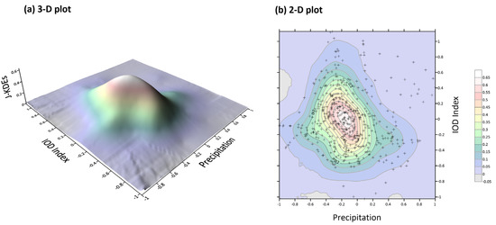
Figure 3.
Lag-1 month nonlinear correlation of joint probability kernel density estimations (J-KDEs) between the normalized three-month moving average precipitation and IOD index in the Korean Peninsula.
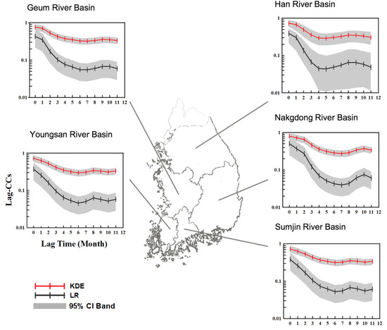
Figure 4.
Non-linear and linear lag-time correlation coefficients (CCs) with 95% confidence limits between IOD index and monthly precipitation for the five major rivers of the Korean Peninsula. Confidence limits are given by 5% and 95% quantiles of 1000 bootstrap resampling replications.
Figure 4 presents the linear and non-linear correlation coefficients (CCs) with their 95% confidence limits between climate indices and precipitation for the five major Korean rivers using the KDE and LR approaches. The lag-0 correlation had the highest correlation for LR and KDE, which was correlated with the IOD index and KP precipitation (LR: 0.315, KDE: 0.684). These time lags indicate a non-linear correlation between climate indices and monthly precipitation; as such, there is a possibility for a diagnostic study on the seasonal or sub-seasonal prediction of local precipitation over the KP using ocean-related large-scale climate indices.
3.2. Evolution Pattern of the Indian Ocean Dipole and Its Local Impacts over the KP
Figure 5 presents analysis results for the change in precipitation in the KP according to the evolution pattern of the p-IOD years from April to November. Total precipitation in the KP decreased significantly from the long-term average, with −11.90% in April–June, −8.63% in May–July, −14.32% in June–August, −9.92% in July–September, −15.23% in August–October, and −7.14% in September–November. The total amount of precipitation change was analyzed using Student’s t-test; it was found that there was a significant decrease in the southern part of the KP at a 95% confidence level. For the p-IOD phases, the pattern of decreased precipitation was more likely to occur at a significant level in the southern part than the mid-northern part of the KP. The changes in this pattern persisted significantly between April and November in the p-IOD years. During the August–October period (autumn in Korea), a distinct pattern of decreased precipitation was observed mainly in the central and southern KP.
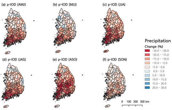
Figure 5.
Evolution pattern of the seasonal precipitation in the KP in the Indian Ocean Dipole mode during p-IOD years. Hatched polygons indicate statistically significant changes of season precipitation at a 5% significance level. Each figure shows seasonal precipitation anomalies over three months, from April to November.
Figure 6 presents the results from the analysis of changes in precipitation in the KP according to the evolution pattern of the n-IOD years from April to November. Total precipitation in the KP tended to decrease or increase more than usual, with −0.71% in April–June, +7.91% in May–July, −1.39% in June–August, −4.05% in July–September, 7.89% in August–October, and −1.07% in September–November. A pattern of significant decreased precipitation in the central part of the KP was observed. However, a pattern of increased precipitation occurred in the southern part of the KP during May–July. For the n-IOD phases, contrary to the p-IOD phases, the pattern of significant decreased precipitation was more likely to appear in the northern KP, as opposed to the central or southern KP. These changes appear to be conspicuous between April and November, when an n-IOD was observed. During p-IOD events (Figure 7a,c), the annual/June–September precipitation in the KP was −7.14%/−14.74% lower than the long-term average annual/June–September precipitation (1971–2000). During n-IOD events (Figure 7b,d), the annual/June–September precipitation in the KP slightly decreased to −1.07%/−3.31%. The composite analysis revealed that the June–September precipitation during p-IOD events was substantially lower than that during long-term normal years. In contrast, n-IOD events had annual/June–September precipitation that was slightly below normal conditions.
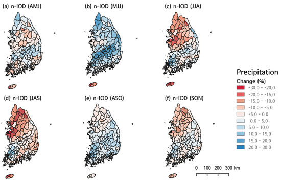
Figure 6.
Evolution pattern of the seasonal precipitation in the KP in the Indian Ocean Dipole mode during n-IOD years. Hatched polygons indicate statistically significant changes of season precipitation at a 5% significance level. Each figure shows seasonal precipitation anomalies over three months, from April to November.
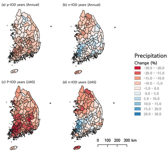
Figure 7.
Composite anomalies of annual and JJAS (June–September) precipitation during p-/n-IOD years. Hatched polygons indicate statistically significant changes in precipitation at a 5% significance level.
The mechanisms of major climate phenomena associated with tropical oceans, such as ENSO and IOD, are not yet fully understood because it is still a challenge to simulate them completely using physical climate models of the global environment. In addition, analyzing and predicting climate phenomena through physical models involves considerable difficulties. Based on the physical model results, applying them to hydrologic circulation systems in a specific EA region, such as KP and China, may follow the problem of scientific reliability and understanding. Therefore, this study analyzed non-linear behavior links with atmospheric teleconnections between hydro-meteorological variables and the climate index using statistical models over the KP with the ocean-related major climate indices, including ENSO and IOD. Statistical approaches have the disadvantage of making it difficult to expect significant levels of results because of the limited number of observations. However, it is one of the most important methods that can be used to complement the prediction results of physical models.
3.3. Nonstationarity of Seasonal Precipitation Anomalies for Different Phases of the IOD
Figure 8 and Figure 9 show changes in the 30-year mean precipitation in five major rivers of the KP. In each figure, Case I shows change over time in the 30-year mean precipitation without excluding the effects of the IOD. Case II is the result of excluding the precipitation in the p-IOD years, and Case III excludes the precipitation in the n-IOD years.
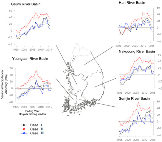
Figure 8.
Changes in seasonal precipitation anomalies (August–October) when the IOD peaked. In each panel, Case I shows the changes over time in the 30-year mean precipitation without excluding the effects of IOD separately. Case II is the result of excluding the precipitation in the positive IOD years, and Case III shows the change in the 30-year mean precipitation, excluding the precipitation in the n-IOD years.
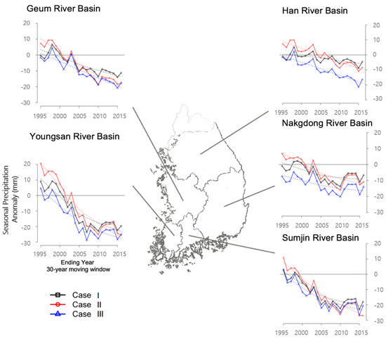
Figure 9.
Changes in seasonal precipitation anomalies (March–May) of the following years when the IOD peaked. In each panel, Case I shows the changes over time in the 30-year mean precipitation without excluding the effects of IOD separately. Case II is the result of excluding the precipitation in the p-IOD years, and Case III shows the change in the 30-year mean precipitation, excluding the precipitation in the n-IOD years.
Figure 8 illustrates the seasonal precipitation from August to October when the IOD peaked; this precipitation from August to October in all five major rivers had a statistically significant increase (p < 0.001). This change in precipitation occurred in the Han River Basin and was relatively abundant in the southern part of the KP. In the Youngsan River Basin, Cases I and III showed a statistically significant increase in the 30-year mean precipitation analysis. Although there was an increase in seasonal precipitation, this change was not statistically significant (p > 0.05). In the Han River Basin, Cases I and II showed statistically significant increases; in contrast, in Case III, there was an increase in seasonal precipitation, although it was not statistically significant (p > 0.05). As shown in the GPCC composite analysis, the p-IOD years in the Youngsan River Basin led to reduced precipitation from the long-term normal throughout the KP. This was particularly the case in the central part of the KP, where a precipitation reduction occurred in the Han River Basin. Notably, the central river basins of the KP (Han and Geum River Basins) have experienced a sharp decline in seasonal precipitation since 2013, and the southern basins have tended to shift from increased seasonal precipitation to declining or plateauing patterns since 2007.
Figure 9 shows changes in the 30-year mean precipitation in March–May, when the IOD crosses the peak and enters a period of decline. The IOD showed a statistically significant decline through the basins of the five rivers, in contrast to precipitation during the peak IOD season. The decline in seasonal precipitation from March–May was noticeable in the Youngsan and Sumjin River Basins in the southern coastal region of Korea.
At times, the IOD co-occurs with ENSO; as such, in this study, the effects of IOD and ENSO on seasonal precipitation changes were analyzed when the IOD peaked, and when the IOD and ENSO entered a period of decline. The effect of the combination of IOD and ENSO is shown in the composite precipitation analysis (Table 1). For the p-IOD phases in the August to October period, the pattern of significant decreases in precipitation was more likely to appear over the entire KP. In contrast, during the p-IOD years, the entire KP experienced precipitation that was 2.6–9.4% greater than the average precipitation in March–May. The occurrence of p-IOD coincided with El Niño events, resulting in more seasonal precipitation in March–May than the occurrence of only p-IODs. This occurred more frequently with cold tongue (CT) El Niño than warm pool (WP) El Niño, resulting in significantly greater spring precipitation across the KP. For the n-IOD years, there was lower precipitation than usual in the Han River Basin (7.4%), followed by the Sumjin River Basin (5.2% reduction in March–May precipitation), and the Youngsan River Basin (3.4% reduction in March–May precipitation). When n-IOD co-occurred with La Niña, there was slightly greater precipitation in March–May than for n-IOD in isolation. These findings indicate that IOD events strongly influence precipitation and its sub-watersheds in the KP. This shows a linkage of possible teleconnections and characteristic changes between tropical Indian-Ocean-related major climactic events and local precipitation variability over the KP.

Table 1.
Changes in seasonal precipitation from the long-term normal (1966–2016) (unit: %).
3.4. Large-Scale Air–Sea Environment and Precipitation Variations over East Asia
Based on the p-IOD and n-IOD years defined above, a composite analysis of autumn (August–October) SSTA in the TIO was conducted (Figure 10). During the p-IOD years, cold SST anomaly patterns appeared in the eastern Indian Ocean, including Indonesia and the maritime continent; warm SSTA patterns emerged in the equatorial region of the Indian Ocean. The warm and cold SST distributions were not extensive, although strong signals were observed in the East Indian Ocean. Conversely, although not strongly dependent on IOD phases, there was a warm and cold SSTA distribution over large areas in the western Indian Ocean. Furthermore, in most areas where warm and cold signals appeared, the confidence level was greater than 95%.
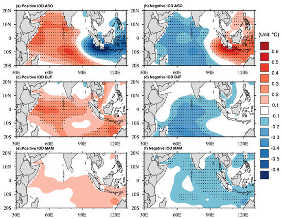
Figure 10.
Composite anomalies of mean SST in the TIO region during positive and negative IOD years, from August to May in the following year. NOAA Extended Reconstructed Sea Surface Temperature version 5 (ERSSTv5) monthly data were used for the SSTA composite analysis; climatology data were used for the normal years from 1956 to 2018. Dotted points indicate values over 95% confidence based on Student’s t-test.
Many recent studies have shown that these different SST anomaly patterns in the TIO region may affect air changes in circulation. Moreover, they detected several teleconnection-based significant changes in different regions of experiencing seasonal precipitation in Northeast Asia. The large-scale physical mechanism of the developing and decaying IOD phases in the atmosphere has not yet been clearly understood. However, there are several reliable studies; some are diagnostic studies, while others are regional impact assessments of the p-IOD and n-IOD [10,17,18,19,20]. After a p-IOD (n-IOD), basin-scale warming (cooling) was referred to as the Indian Ocean Basin (IOB) mode [32]. These influences on the IOB may affect the climate of EA in the following season.
Figure 11 shows the composite anomalies (1981–2010 climatology) of the GPCC precipitation and 850 hPa wind over northeast Asia during strong IOD events, in the same way as SSTA. During the warm boreal season, southwesterly winds from the Indian Ocean and the South China Sea (SCS) were dominant and advected a large amount of moisture from the Indian Ocean to EA [34]. In p-IOD (n-IOD) years, there was an anticyclonic (cyclonic) circulation in the SCS. This large circulation may help to transport (prevent) moisture to EA. The composite precipitation anomalies of p-IOD (n-IOD) years showed that they were above (below) normal over the southern parts of China. In contrast, other parts of EA, including the KP, experienced drier (wetter) signals than normal years (Figure 11a,b). In p-IOD years, southern China and the SCS are mainly affected by the southwesterly winds, and this pattern continues until the following spring. In particular, heavy precipitation occurred in southern China during the boreal winter season; this is consistent with the findings of Qui et al. [35]. During n-IOD years, easterly winds were observed in EA (Figure 11e–h).
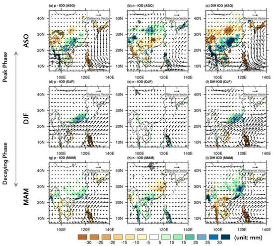
Figure 11.
Composite anomalies of the GPCC precipitation and 850 hPa low-level wind anomalies from autumn (August–September–October) to spring (March–April–May) of the following year during IOD events over the northeast Asia region. The left (middle) panel indicates the p-IOD (n-IOD) events, and the right panel shows the large-scale circulation differences between p-IOD and n-IOD years. Dots denote values over 95% confidence based on Student’s t-test.
4. Conclusions
Understanding the relationship between air–sea environments and precipitation variations in EA for areas experiencing high seasonal variability and uncertainty regarding seasonal precipitation data is critical to develop a sustainable freshwater management system. In this study, statistical models were used to analyze non-linear behavior links of atmospheric teleconnections between climate indices and seasonal precipitation. The IOD mode, a major ocean-related climatic factor in the Indian Ocean, was used to analyze long-term changes in seasonal precipitation over the EA region. The primary results are summarized as follows:
- (1)
- The analysis of atmospheric teleconnections was conducted using PCA and SSA techniques. Non-linear lag correlations between climate indices and seasonal precipitation were calculated using the MI technique, and their lag-time correlations were simulated from lag-0 to lag-11. Teleconnection-based non-linear and linear CCs were conducted between climate indices and seasonal precipitation using LR and KDE based on the MI results. Results from non-linear CCs were higher than those from linear correlations, and IOD was found to directly influence the precipitation anomaly time series over the KP. This study demonstrates a method for teleconnection-based long-range water resource management to reduce climate uncertainty when an abnormal SSTA occurs in the TIO region;
- (2)
- When the IOD reached its peak (August to October), a significant decrease in seasonal precipitation during the n-IOD period was observed throughout the KP. For the spring period (March to May), seasonal precipitation during p-IOD years coincided with the El Niño phenomenon, which was higher than those of only p-IOD years. These changes occurred more frequently in the CT El Niño than in the WP El Niño years. For the co-occurrence of n-IODs and La Niña, there was greater precipitation than when only n-IODs occurred in isolation;
- (3)
- The characteristics of non-stationary 30-year averaged seasonal precipitation were detected throughout the KP. The precipitation in autumn (August to October) was observed to increase significantly (p < 0.001) when excluding the p-IOD year across the KP. In contrast, seasonal precipitation in the central river basins of KP had plummeted since 2013 and decreased in the southern basins of the KP since 2007. Spring precipitation showed statistically significant declines across the five major rivers in the KP when IODs peaked and entered a period of decline. The decline in seasonal precipitation from March to May was noticeable in the southern coastal regions of Korea;
- (4)
- During p-IOD years, there were more precipitation signals than usual in the southern part of China, including the SCS and the southern part of Japan, with cyclonic circulation patterns. A high-pressure anti-cyclonic pattern was observed over eastern China and the KP. There was a drier signal in n-IOD years than normal in the SCS and southern China, along with a high-pressure anti-cyclonic pattern. Conversely, inland and eastern regions of China and Japan showed wetter signals than usual, with a cyclonic circulation pattern. However, the KP was located between the two cyclonic circulations, and the district precipitation signal was not visible. The signal was less dry than the p-IOD years.
The results of this diagnostic study may be utilized in decision-making processes to minimize climate-related disasters, such as floods and droughts, through seasonal prediction. Additionally, these results may inform the development of optimal strategies to ensure best management practices for water use under a changing climate.
Author Contributions
Conceptualization, resources, formal analysis, writing—original draft, J.-S.K., S.-K.Y., and S.-M.O.; data curation, methodology; J.-S.K. and S.-K.Y., writing-review and editing; J.-S.K., S.-K.Y., and H.C. All authors have read and agreed to the published version of the manuscript.
Funding
The APC was funded by Seoul Institute of Technology (2020-AB-001), Seoul, South Korea, and partially supported by the Korea Meteorological Administration Research and Development Program “Development of Marine Meteorology Monitoring and Next-generation Ocean Forecasting System” under Grant (KMA2018-00420).
Data Availability Statement
The authors acknowledge the monthly SST data from the National Oceanic and Atmospheric Administration (NOAA) and the monthly vector wind anomalies at 850 hPa provided by the National Centers for Environmental Prediction and the National Center for Atmospheric Research (NCEP-NCAR) reanalysis, version 2 at https://www.ncdc.noaa.gov/data-access/model-data/model-datasets/reanalysis-1-reanalysis-2 (accessed on 5 May 2021). The monthly Indian Ocean Dipole Mode Index (DMI) data were obtained from the Japan Agency for Marine-Earth Science and Technology (JAMSTEC) at http://www.jamstec.go.jp/frsgc/research/d1/iod/iod_home.html.en (accessed on 5 May 2021), Japan, and the Hadley Centre Sea Ice and Sea Surface Temperature dataset (HadISST) by the NOAA Climate Prediction Center (CPC) at https://www.cpc.ncep.noaa.gov/ (accessed on 5 May 2021). The monthly precipitation dataset by the Global Precipitation Climatology Center (GPCC) from Deutscher Wetterdienst in Germany at https://climatedataguide.ucar.edu/climate-data/gpcc-global-precipitation-climatology-centre (accessed on 5 May 2021). The authors also acknowledged that the local precipitation data for 117 sub-watersheds of the five major river basins over the KP by the Water Resources Management Information System (WAMIS) at http://www.wamis.go.kr/ (accessed on 5 May 2021), and the multi-model ensemble climate data provided by the APEC Climate Center (APCC) at http://www.apcc21.org/ (accessed on 5 May 2021).
Acknowledgments
This work was supported by the Seoul Institute of Technology, Seoul, South Korea, and the third author, Sang-Myeong Oh, was acknowledged the Korea Meteorological Administration Research and Development Program by the Korea Meteorological Administration (KMA), South Korea. We also appreciate the support of the State Key Laboratory of Water Resources and Hydropower Engineering Science, Wuhan University, China. The authors thank the three anonymous reviewers for their comments and valuable suggestions.
Conflicts of Interest
The authors declare no conflict of interest.
References
- Wang, B.; Wu, R.; Fu, X. Pacific-East Asia Teleconnection: How Does ENSO Affect East Asian Climate? J. Clim. 2000, 13, 1517–1536. [Google Scholar] [CrossRef]
- Pizarro, G.; Lall, U. El Niño-induced flooding in the U.S. West: What can we expect? Eos Trans. Am. Geophys. Union. 2002, 83, 349–352. [Google Scholar] [CrossRef]
- IPCC (Intergovernmental Panel on Climate Change). Managing the Risks of Extreme Events and Disasters to Advance Climate Change Adaptation (SREX)—Special Report of the Intergovernmental Panel on Climate Change; Cambridge University Press: Cambridge, UK, 2007; pp. 1–594. [Google Scholar]
- Horel, J.D.; Wallace, J.M. Planetary-scale atmospheric phenomena associated with the Southern Oscillation. Mon. Weather Rev. 1981, 109, 813–829. [Google Scholar] [CrossRef]
- Kim, J.S.; Jain, S.; Yoon, S.K. Warm season streamflow variability in the Korean Han River Basin: Links with atmospheric teleconnections. Int. J. Clim. 2012, 32, 635–640. [Google Scholar] [CrossRef]
- Yoon, S.K.; Kim, J.S.; Lee, J.H.; Moon, Y.I. Hydrometeorological variability in the Korean Han River Basin and its sub-watersheds during different El Niño phases. Stoch. Environ. Res. Risk Assess. 2013, 27, 1465–1477. [Google Scholar] [CrossRef]
- Lee, T.S.; Ouarda, T.; Yoon, S.K. KNN-based Local Linear Regression for the Analysis and Simulation of Low Flow Extremes under Climatic Influence. Clim. Dyn. 2017, 49, 3493–3511. [Google Scholar] [CrossRef]
- Piechota, T.C.; Dracup, J.A. Drought and regional hydrologic variation in the United States: Associations with the El Niño-Southern Oscillation. Water Resour. Res. 1996, 32, 1359–1373. [Google Scholar] [CrossRef]
- Piechota, T.C.; Chiew, H.S.; Francis Dracup, J.A.; McMachon, T.A. Seasonal streamflow forecasting in eastern Australia and the El Niño-Southern Oscillation. Water Resour. Res. 1998, 34, 3035–3044. [Google Scholar] [CrossRef]
- Saji, N.H.; Goswami, B.N.; Vinayachandran, P.N.; Yamagata, T. A dipole mode in the tropical Indian Ocean. Nature 1999, 401, 360–363. [Google Scholar] [CrossRef] [PubMed]
- Yoon, S.K.; Lee, T. Investigation of hydrological variability in the Korean Peninsula with the ENSO teleconnections. Proc. Int. Associ. Hydrol. Sci. 2016, 374, 165–173. [Google Scholar] [CrossRef]
- Kim, J.-S.; Xaiyaseng, P.; Xiong, L.; Yoon, S.-K.; Lee, T. Remote Sensing-Based Rainfall Variability for Warming and Cooling in Indo-Pacific Ocean with Intentional Statistical Simulations. Remote Sens. 2020, 12, 1458. [Google Scholar] [CrossRef]
- Ashok, K.; Guan, Z.; Yamagata, T. Influence of the Indian Ocean dipole on the Australian winter rainfall. Geophys. Res. Lett. 2003, 30, 1821. [Google Scholar] [CrossRef]
- McPhaden, M.J.; Zebiak, S.E.; Glantz, M.H. ENSO as an integrating concept in Earth Science. Science 2006, 314, 1740–1745. [Google Scholar] [CrossRef] [PubMed]
- Pradhan, P.K.; Preethi, B.; Ashok, K.; Krishna, R.; Sahai, A.K. Modoki, Indian Ocean Dipole, and western North Pacific typhoons, Possible implications for extreme events. J. Geophys. Res. 2011, 116, D18108. [Google Scholar] [CrossRef]
- Klein, S.A.; Soden, B.J.; Lau, N.C. Remote sea surface temperature variations during ENSO, Evidence for a tropical atmospheric bridge. J. Clim. 1999, 12, 917–932. [Google Scholar] [CrossRef]
- Lau, N.C.; Nath, M.J. Atmosphere-ocean variations in the Indo-Pacific sector during ENSO episodes. J. Clim. 2003, 16, 3–20. [Google Scholar] [CrossRef]
- Behera, S.K.; Krishnan, R.; Yamagata, T. Unusual ocean-atmosphere conditions in the tropical Indian Ocean during 1994. Geophys. Res. Lett. 1999, 26, 3001–3004. [Google Scholar] [CrossRef]
- Webster, P.J.; Moore, A.M.; Loschnigg, J.P.; Leben, R.R. Coupled ocean–atmosphere dynamics in the Indian Ocean during 1997–98. Nature 1999, 401, 356–360. [Google Scholar] [CrossRef] [PubMed]
- Saji, N.H.; Yamagata, T. Structure of SST and Surface Wind Variability during Indian Ocean Dipole Mode Events, COADS Observations. J. Clim. 2003, 16, 2735–2751. [Google Scholar] [CrossRef]
- Liu, Y.; Yoon, S.-K.; Kim, J.-S.; Xiong, L.; Lee, J.-H. Changes in Intensity and Variability of Tropical Cyclones over the Western North Pacific and Their Local Impacts under Different Types of El Niños. Atmosphere 2021, 12, 59. [Google Scholar] [CrossRef]
- Enomoto, T.; Hoskins, B.J.; Matsuda, Y. The formation of the Bonin high in August. Q. J. R. Meteorol. Soc. 2003, 587, 157–178. [Google Scholar] [CrossRef]
- Guan, Z.; Yamagata, T. The unusual summer of 1994 in East Asia: IOD Teleconnections. Geophys. Res. Lett. 2003, 30, 1544. [Google Scholar] [CrossRef]
- Cherchi, A.; Annamalai, H.; Masina, S.; Navarra, A.; Alessandri, A. Twenty-first century projected summer mean climate in the Mediterranean interpreted through the monsoon-desert mechanism. Clim. Dyn. 2016, 47, 2361–2371. [Google Scholar] [CrossRef]
- Zhang, Y.; Zhou, W.; Chow, E.C.H.; Leung, M.Y. Delayed impacts of the IOD: Cross-seasonal relationships between the IOD, Tibetan Plateau snow, and summer precipitation over the Yangtze–Huaihe River region. Clim. Dyn. 2019, 53, 4077–4093. [Google Scholar] [CrossRef]
- Weng, H.; Wu, G.; Liu, Y.; Behera, S.K.; Yamagata, T. Anomalous summer climate in China influenced by the tropical Indo-Pacific Oceans. Clim. Dyn. 2011, 36, 769–782. [Google Scholar] [CrossRef][Green Version]
- Cai, W.; van Rensch, P.; Cowan, T.; Hendon, H.H. Teleconnection pathways of ENSO and the IOD and the mechanisms for impacts on Australian rainfall. J. Clim. 2011, 24, 3910–3923. [Google Scholar] [CrossRef]
- Kosaka, Y.; Xie, S.P. Recent global-warming hiatus tied to equatorial Pacific surface cooling. Nature 2013, 501, 403–407. [Google Scholar] [CrossRef] [PubMed]
- Lee, S.K.; Park, W.; Baringer, M.O.; Gordon, A.L.; Huber, B.; Liu, Y. Pacific origin of the abrupt increase in Indian Ocean heat content during the warming hiatus. Nat. Geosci. 2015, 8, 445–449. [Google Scholar] [CrossRef]
- Liu, W.; Xie, S.P.; Lu, J. Tracking ocean heat uptake during the surface warming hiatus. Nat. Commun. 2016, 7, 10926. [Google Scholar] [CrossRef]
- Zheng, X.T.; Xie, S.P.; Liu, Q. Response of the Indian Ocean Basin Mode and Its Capacity Effect to Global Warming. J. Clim. 2012, 24, 6146–6164. [Google Scholar] [CrossRef]
- Qu, X.; Huang, G. An Enhanced Influence of Tropical Indian Ocean on the South Asia High after the Late 1970s. J. Clim. 2012, 25, 6930–6941. [Google Scholar] [CrossRef]
- Roxy, M.K.; Gnanaseelan, C.; Parekh, A.; Chowdary, J.S.; Singh, S.; Modi, A.; Kakatkar, R.; Mohapatra, S.; Dhara, C.; Shenoi, S.C.; et al. Indian Ocean Warming. In Assessment of Climate Change over the Indian Region; Krishnan, R., Sanjay, J., Gnanaseelan, C., Mujumdar, M., Kulkarni, A., Chakraborty, S., Eds.; Springer: Singapore, 2020. [Google Scholar] [CrossRef]
- Moon, Y.I.; Lall, U. Atmospheric flow indices and interannual Great Salt Lake variability. J. Hydrol. Eng. 1996, 1, 55–62. [Google Scholar] [CrossRef]
- Moon, Y.I.; Rajagopalan, B.; Lall, U. Estimation of mutual information using kernel density estimators. Phys. Rev. E 1995, 52, 2318–2321. [Google Scholar] [CrossRef] [PubMed]
- Martinerie, J.M.; Albano, A.M.; Mees, A.I.; Rapp, P.E. Mutual Information, Strange Attractors, and the Optimal Estimation of Dimension. Phys. Rev. A 1992, 45, 7058–7064. [Google Scholar] [CrossRef] [PubMed]
- Gao, J.; Zheng, Z. Direct dynamical test for deterministic chaos and optimal embedding of a chaotic time series. Phys. Rev. E 1994, 49, 3807. [Google Scholar] [CrossRef]
- Joe, H. Relative entropy measures of multivariate dependence. J. Am. Stat. Assoc. 1989, 84, 157–164. [Google Scholar] [CrossRef]
- Granger, C.; Lin, J. Using the mutual information coefficients to identify lags in nonlinear models. J. Time. Ser. Anal. 1994, 15, 371–384. [Google Scholar] [CrossRef]
- Chavez, M.; Cazelles, B. Detecting dynamic spatial correlation patterns with generalized wavelet coherence and non-stationary surrogate data. Sci. Rep. 2019, 9, 7389. [Google Scholar] [CrossRef]
- Yu, B.; Lupo, A.R. Large-Scale Atmospheric Circulation Variability and Its Climate Impacts. Atmosphere 2019, 10, 329. [Google Scholar] [CrossRef]
- Perlwitz, J.; Knutson, T.; Kossin, J.P.; LeGrande, A.N. Large-scale circulation and climate variability. In Climate Science Special Report: Fourth National Climate Assessment, Volume I; Wuebbles, D.J., Fahey, D.W., Hibbard, K.A., Dokken, D.J., Stewart, B.C., Maycock, T.K., Eds.; U.S. Global Change Research Program: Washington, DC, USA, 2017; pp. 61–184. [Google Scholar] [CrossRef]
- Yang, J.; Liu, Q.; Xie, S.-P.; Liu, Z.; Wu, L. Impact of the Indian Ocean SST basin mode on the Asian summer monsoon. Geophys. Res. Lett. 2007, 34, L02708. [Google Scholar] [CrossRef]
- Yuan, Y.; Yang, H.; Zhou, W.; Li, C. Influences of the Indian Ocean dipole on the Asian summer monsoon in the following year. Int. J. Clim. 2008, 28, 1849–1859. [Google Scholar] [CrossRef]
- Qui, Y.; Cai, W.; Guo, X.; Ng, B. The asymmetric influence of the positive and negative IOD events on China’s rainfall. Sci. Rep. 2014, 4, 4943. [Google Scholar] [CrossRef]


Publisher’s Note: MDPI stays neutral with regard to jurisdictional claims in published maps and institutional affiliations. |
© 2021 by the authors. Licensee MDPI, Basel, Switzerland. This article is an open access article distributed under the terms and conditions of the Creative Commons Attribution (CC BY) license (https://creativecommons.org/licenses/by/4.0/).