Article

Deep Learning and Phenology Enhance Large-Scale Tree Species Classification in Aerial Imagery during a Biosecurity Response

1
Scion, Private Bag 3020, Rotorua 3046, New Zealand
2
Scion, 10 Kyle Street, Christchurch 8011, New Zealand
*
Author to whom correspondence should be addressed.
Remote Sens. 2021, 13(9), 1789; https://doi.org/10.3390/rs13091789
Submission received: 17 April 2021 / Revised: 29 April 2021 / Accepted: 29 April 2021 / Published: 4 May 2021
(This article belongs to the Special Issue Mapping Tree Species Diversity)

Abstract

:
The ability of deep convolutional neural networks (deep learning) to learn complex visual characteristics offers a new method to classify tree species using lower-cost data such as regional aerial RGB imagery. In this study, we use 10 cm resolution imagery and 4600 trees to develop a deep learning model to identify Metrosideros excelsa (pōhutukawa)—a culturally important New Zealand tree that displays distinctive red flowers during summer and is under threat from the invasive pathogen Austropuccinia psidii (myrtle rust). Our objectives were to compare the accuracy of deep learning models that could learn the distinctive visual characteristics of the canopies with tree-based models (XGBoost) that used spectral and textural metrics. We tested whether the phenology of pōhutukawa could be used to enhance classification by using multitemporal aerial imagery that showed the same trees with and without widespread flowering. The XGBoost model achieved an accuracy of 86.7% on the dataset with strong phenology (flowering). Without phenology, the accuracy fell to 79.4% and the model relied on the blueish hue and texture of the canopies. The deep learning model achieved 97.4% accuracy with 96.5% sensitivity and 98.3% specificity when leveraging phenology—even though the intensity of flowering varied substantially. Without strong phenology, the accuracy of the deep learning model remained high at 92.7% with sensitivity of 91.2% and specificity of 94.3% despite significant variation in the appearance of non-flowering pōhutukawa. Pooling time-series imagery did not enhance either approach. The accuracy of XGBoost and deep learning models were, respectively, 83.2% and 95.2%, which were of intermediate precision between the separate models.

Graphical Abstract

1. Introduction

The early stages of a biosecurity response to a newly arrived plant pathogen can have a significant bearing on the final outcome and cost [1,2]. Once an unwanted pathogen has been positively identified, mapping and identification of potential host species become essential for managing the incursion [3]. Identification of host plants must be carried out by trained personnel and the hosts may be located across a mixture of public and private property or in hard to access areas. For these reasons, carrying out large-scale searches for host plants can be very costly and challenging to resource.
The level of host detection and surveillance required in the face of an incursion is usually defined by the response objective. Eradication of a pathogen necessitates exhaustive detection of host species to monitor spread and enable the destruction of infected plants or even hosts showing no signs of infection to limit future spread. A monitoring objective may require only the identification of key indicator species to define the infection front and monitor impacts and host range. Finally, long-term management strategies may require large-scale but inexhaustive host identification to locate resistant individuals within a population for breeding programmes or other approaches to biological control [4,5].
Remote sensing can complement all of these objectives by offering an efficient and scalable means of identifying host species [6,7]. Imagery acquired from UAVs, aircraft or even space-borne optical sensors can be used to identify both potential hosts as well as the symptoms of pathogen infection on susceptible host species [6,8]. However, the detection and classification of species from remotely sensed data comprise a complex sub-discipline. Fassnacht et al. [9] carried out a comprehensive review of methods for tree species classification using remotely sensed data and highlighted clear themes in the literature. Multispectral and hyperspectral data were identified as being the most useful data sources for accurate species classification with LiDAR data being highly complementary. Through capturing reflected light outside the visible spectrum, the use of multi/hyperspectral data sources increases the chance of observing patterns of reflectance related to structural or biochemical traits that may be unique or distinctive to species or groups.
Multispectral data (4–12 bands) are relatively easy to capture and have been widely used in combination with machine learning methods to perform species classification [10,11,12]. However, accurate classification is often limited to broad groups such as conifer vs. deciduous forest types [13]. Hyperspectral data contain many more (>12) narrow spectral bands—enhancing the ability to observe small differences that may be present between the spectra of tree species and has been well studied for fine-grained species classification tasks [14,15]. The idea of unique spectral ‘signatures’ for species has been present in the literature for several decades; however, [9] concluded that these signatures appear to be rare in practice and, when present, require observation of a wide portion of the spectrum using sophisticated sensors [16].
Although hyperspectral data have been successfully used to classify as many as 42 species [6,9,17], large-scale applications of hyperspectral-based species classification face challenges related to practicality and cost. The increased spectral resolution usually demands careful acquisition from expensive sensors and is constrained by illumination and atmospheric requirements. The post-processing of these data can also be complex and requires careful correction of atmospheric impacts and noise reduction. Finally, the substantial volumes of data must often be subjected to dimensionality reduction before analysis can proceed [13,18]. Classification is based on patterns in the calibrated reflectance spectra from the canopy and differences in data sources and quality can reduce the transferability of the classifiers [19]. Other information content, such as the structure, shape, texture and other distinctive but hard to quantify characteristics are often neglected or partially utilised. Efforts to characterise the texture or the shape of the crown or other attributes typically rely on a small number of engineered features to summarise complex attributes [11,13].
In contrast, the human visual system allows experienced individuals to distinguish many species by visual inspection alone. Some cryptic species remain hard to tell apart visually, but trained experts (and even non-experts) can discriminate a surprising number of species [20]. This has led to the development of sites such as iNaturalist, where members of the public can upload images of species for experts to identify [21]. Recently, the advent of deep learning models based on convolutional neural networks (hereafter referred to as deep learning) has transformed the capability of machines to perform fine-grained classification of images, often reaching or exceeding human-level accuracy [22,23]. The architecture of these networks allows these networks to effectively learn the features important for classification. This is an important contrast with other approaches as the features are not engineered or pre-selected but rather learned by the network from labelled training examples with little requirement for image pre-processing.
Deep learning has been used for tree species classification from various combinations of LiDAR, hyperspectral and multispectral imagery [24,25,26,27]. Many studies have also successfully used simpler RGB imagery for species detection and classification. Importantly, these approaches have demonstrated a remarkable capacity to perform fine-grained species classification from consumer-grade camera imagery that is poorly suited to traditional remote sensing [28,29]. However, these studies have mostly used RGB data collected from UAV [30,31,32] and to a lesser extent high-resolution satellites [33,34], which constrains the ability to scale predictions in the former case or limits the spatial resolution of predictions in the latter case.
Although RGB imagery is routinely captured at regional levels by fixed-wing aircraft in many countries, few studies have undertaken large-scale host species identification using this ubiquitous data source. These data often include only RGB colour channels in uncalibrated radiance values rather than reflectance. The simplicity of these data means that large areas can be captured at high-resolution (<10 cm) for lower unit cost. Successful application of deep learning for large-scale host species identification using aerial imagery offers a scalable method to support biosecurity responses that bypasses many issues facing ground-based surveillance such as permissions and safe accessibility.
Classification of tree species is generally enhanced when there is low spectral variability within a species and high spectral variability between the target and other species [35]. Often there are times during the year when interspecies spectral variability is greater because of variation in phenological attributes such as leaf flush, senescence, or flowering. Little research has examined how phenological variation can be used by deep learning to improve species classification in trees, although we are aware of one such study for an invasive weed [36]. Collection of data from a species during a period of distinctive phenology could assist the use of deep learning through both enhancing predictive precision and providing a means to rapidly generate large training datasets.
Myrtle rust, caused by the fungal plant pathogen Austropuccinia psidii (G. Winter) Beenken (syn. Puccinia psidii), affects a broad range of hosts in the Myrtaceae family, causing lesions, dieback and, in some cases, mortality [37,38]. The pathogen is airborne and has spread rapidly around the globe [39,40,41,42]. New Zealand is home to at least 37 native myrtaceous species [43]. Of these, Metrosideros excelsa Sol. Ex Gaertn (pōhutukawa) has very high cultural value and has been widely planted for amenity purposes. This coastal evergreen tree has a sprawling habit of up to 20 m and produces dense masses of red flowers over the Christmas period [44], earning it the name ‘the New Zealand Christmas tree’. Observations from pōhutukawa growing in other countries where myrtle rust is present indicate that the species is susceptible to myrtle rust [45,46].
In May 2017, myrtle rust was detected on the New Zealand mainland for the first time [47]. The disease has spread rapidly and has established on numerous native and exotic host species [48].
The overarching goal of this research was to test novel methods suitable for large-scale identification of key Metrosideros host species focussing on pōhutukawa as a test case. Specifically, the objectives of the research were to (1) test two state-of-the-art classification methods (XGBoost and deep convolutional neural networks) applied to three-band aerial imagery leveraging the strong phenology of pōhutukawa, i.e., distinctive flowering in summer, (2) test classification of the same trees without the assistance of phenology by using historical aerial imagery (3) test how practical and generally applicable these techniques are in real-world conditions by creating a combined dataset from objectives 1 and 2 that contained imagery captured using different sensors in different years and that showed a mixture of flowering and non-flowering trees.

2. Materials and Methods

2.1. Ground Truth Data

New Zealand maintains an extensive biosecurity surveillance system and an established incursion response protocol. During the first months after the incursion of myrtle rust, sites that were confirmed to contain infected hosts received intensive ground-based surveys to identify and inspect all potential host species within a fixed radius from the infected site. New, confirmed infections triggered additional searches around the new site. A mobile app used by trained inspectors was used to record the genus, GPS location and infection status for every host inspected during the response. These efforts produced a substantial volume of ground surveillance data including GPS locations and positive identification of Metrosideros spp. by trained inspectors. Many of the trees inspected were present within the coastal city of Tauranga (Figure 1), and nearly all the records for Metrosideros spp. in this region were pōhutukawa.
The extensive and distinctive red flowers of pōhutukawa are easily identifiable from above in the summer which made this species an ideal candidate to test the potential to utilise phenology to enhance species identification in RGB aerial imagery. For much of the rest of the year, some degree of buds, flowers, or seed capsules are present but less distinctive. However, the multi-leader crown shape and blueish hue of the large, waxy and elliptical leaves are also distinctive and present all year round (Figure 2).
Aerial imagery captured over Tauranga during the 2018–2019 summer period (Table 1) was overlaid with the ground surveillance locations in a GIS. Locations were collected using consumer-grade GPS and could only be considered approximate.
For each inspection record, a trained analyst examined the GPS point and identified the corresponding tree in the aerial imagery. If the tree showed at least some evidence of flowering, then the imagery was annotated by delineating a bounding box around the canopy extent. The distinctive features of the canopy and strong flowering observed in the imagery greatly assisted identification and annotation; however, inspection records were only at the genus level and other species with similar phenological traits such as Metrosideros robusta (rātā) may occasionally be found within this region. In addition, some cultivated Metrosideros excelsa ‘Aurea’ (‘yellow’ pōhutukawa) appeared to be present within the dataset but these were removed due to the small number of samples available.
We assessed the purity of the training dataset by inspecting the majority of trees using publicly available, street-level imagery followed by on-site inspections for a smaller subset of trees. The results show that all study trees identified through combining the aerial imagery and surveillance records were pōhutukawa. After completing this process, we considered that the assembled training dataset consisted of only pōhutukawa and any misclassifications would have been very small in number.
Development of the classifiers also required negative examples. The candidate negative examples were any tree other than Metrosideros spp., hereafter referred to as other species. We once again leveraged the ground inspection efforts to develop this dataset. The intensity of the initial surveillance efforts meant that within inspected areas, such as streets or parks, the locations for nearly every pōhutukawa were recorded. We used these areas to select negative examples and cross-referenced a substantial portion of the dataset against other imagery and field inspections. This approach reduced the chances of accidentally including pōhutukawa or biasing the training set by excluding species that were visually similar to pōhutukawa due to uncertainty. In addition, this provided a realistic set of non-target tree canopies that the classifier might encounter in the areas surveyed for the biosecurity response. Bounding boxes around the canopies were defined against the aerial imagery and annotation proceeded until the dataset was balanced. Figure 3 shows examples of typical and atypical pōhutukawa and other tree species as seen in the aerial imagery.

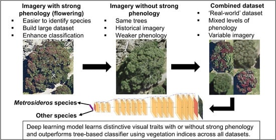
2.2. Imagery Datasets

The aerial imagery datasets consisted of large orthomosaics generated from campaigns carried out in 2017 and 2019 using different aerial cameras (Table 1). The imagery from 2017 showed lower levels of detail, probably due to poorer image matching, and the trees had less visual detail (Figure 3). The bounding boxes were used to extract sub-images from the larger orthomosaics and each image ‘chip’ showing a tree canopy was labelled with the dataset year and class (pōhutukawa or other spp.). Very small trees (canopy radius < ~1.5m) were excluded as these canopies contained too few pixels.
The final datasets included 2300 images of tree canopies evenly split between pōhutukawa and other spp. with images available for both 2017 and 2019 (Table 2). Images of pōhutukawa from 2019 and 2017 were used, respectively, to test the classification with and without the assistance of strong phenological features (Table 2). The imagery from the 2017 and 2019 datasets was combined to assess how well the model would generalise under real-world conditions (Table 2). The images of tree canopies were randomly split into training data (70%) used to fit the models. Validation data (15%) were used to select hyperparameters and evaluate model performance during training and a test set (15%) was used to assess final model performance on completely withheld data (Table 2). Trees were assigned to the same splits in the 2017 and 2019 datasets for a fair comparison of the models. For the combined dataset, data were re-shuffled at the tree level and the imagery from both years was included in the assigned split to prevent data leakage.

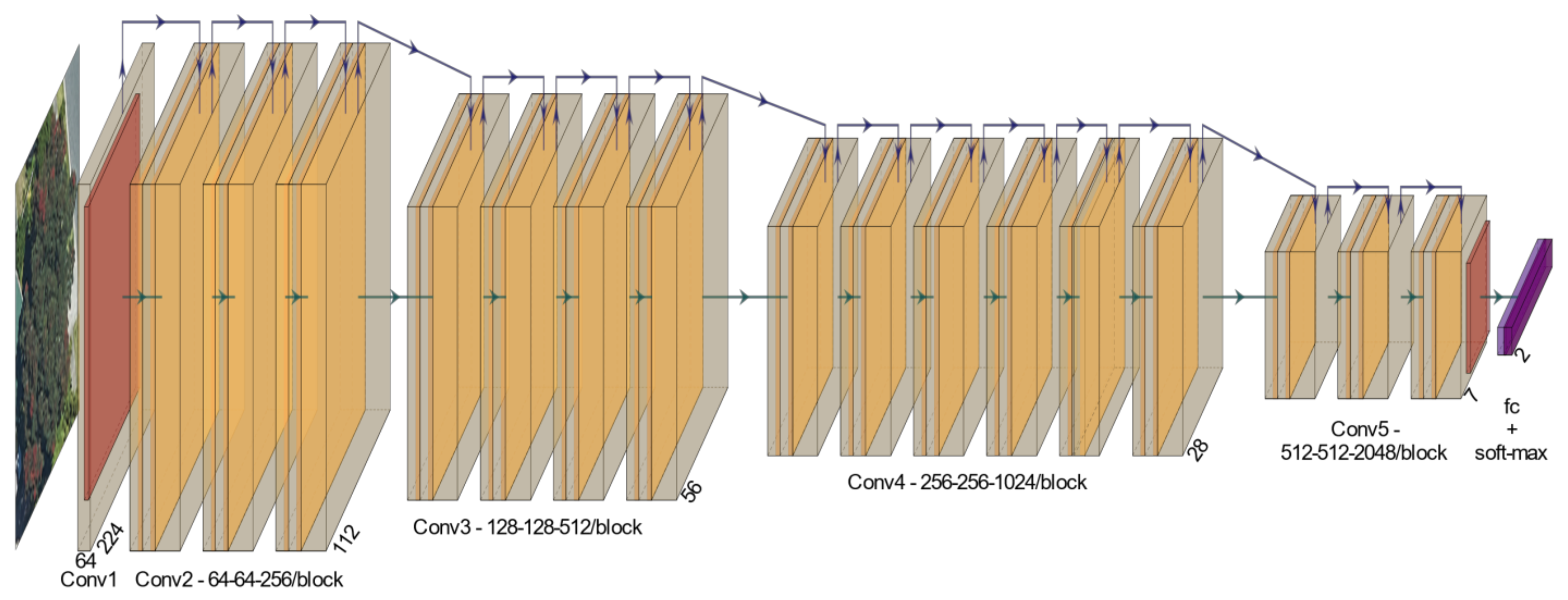
2.3. Deep Learning Models

We selected the ResNet model architecture [49] for classification of the tree canopies. The ResNet model is made up of small building blocks called the residual block. Each residual block is primarily made up of two to three convolution layers (this is dependent on the depth of the network) stacked together. The convolution layers are designed to learn and fit against the residual of the target function. The learned residual is then mapped back to the learned function through a skip connection that connects the input of the residual block to the output of the stacked convolution layers. By designing the neural network to learn and optimise on the residual instead of the original function, ResNet can learn the unknown original function more easily, thereby improving accuracy. We used the ResNet-50 architecture, which comprises 49 convolution layers organised into residual blocks and a fully connected layer for classification (Figure 4).
A randomly initialized, fully connected layer was trained for 2 epochs to adapt a model pre-trained on the ImageNet [50] task to the binary classification task in this study. Thereafter, differential learning rates in the range 1 × 10⁻³–1 × 10⁻⁶ were used to adapt deeper layers of the network at linearly decreasing learning rates for another 30 epochs. At this point, the performance validation metrics showed no further benefits from additional training. All deep learning models and metrics were implemented using the PyTorch 1.4 deep learning library [51] and the Scikit-Learn Python package [52]. Model training was carried out using a Nvidia Tesla K80 GPU with 12 GB of memory.

2.4. XGBoost Models

Approaches to species classification frequently use imagery to generate variables (metrics), such as vegetation indices, to capture features or characteristics useful for discriminating different species [9,13]. This may be done using rule-based methods [53] or machine learning methods such as decision trees [54]. We chose variables that target the distinctive properties of pōhutukawa canopies. These included spectral metrics aimed at capturing the blueish hue of the leathery, elliptical leaves and the strong and distinctive sprays of red flowers present in summer. The canopies also exhibit distinctive textural properties arising from the multi-stem structure and leaf and bud arrangements independent of the presence or absence of flowers (Figure 2 and Figure 3). Texture analysis using grey-level co-occurrence matrices (GLCMs) [55] was used to try and capture these characteristics. Computation of the texture images was done using the ‘glcm’ package [56] in R [57]. The GLCM metric classes and parameters were selected based on the analysis and recommendations of [58]. The raw digital numbers (pixel radiance values) within each canopy bounding box were used to generate patch-level mean values for the predictive variables (Table 3). This was necessary because this type of imagery is optimised for visual appearance and lacks the information required to calculate reflectance.
We selected the XGBoost algorithm to perform binary classification using the ‘xgboost’ package for R [59]. XGBoost is a tree-based machine learning algorithm that is scalable, fast and has produced benchmark results on classification tasks [60]. The spectral and textural variables were used to train the XGBoost classifier for a maximum of 400 iterations, with early stopping based on validation set metrics used to prevent over-fitting. Subsampling of variables and observations for individual tree learners was also implemented alongside fine-tuning of the gamma hyperparameter to further guard against over-fitting.

2.5. Performance Metrics

The predictions made by the final models on the withheld test splits of the three imagery datasets were used to compute the number of correct classifications (true positives) and incorrect classifications (false positives) for the pōhutukawa and ‘other spp.’ classes. These values were used to compute the classification performance metrics shown in Table 4.

3. Results

3.1. XGBoost Models

The results from the XGBoost and deep learning models applied to the withheld portions of the datasets used to test classification with phenology (2019 imagery), without phenology (2017 imagery) and classification of the combined datasets are shown in Table 5. The XGBoost classifiers showed moderately high accuracy on all three datasets (Table 5). The strong phenological traits of the pōhutukawa captured in the 2019 summer imagery produced the model with the highest accuracy (86.7%). The sensitivity and specificity were similar, reflecting nearly equal rates of false negatives and false positives. The variable importance scores extracted from XGBoost are shown in Figure 5. The scaled green pixel values and the RG ratio metric capturing the ratio of red to green pixels had the highest importance in the 2019 model utilising phenology. These two metrics most likely captured differences between the mostly green canopies of other spp. and the extensive showers of red flowers present on many pōhutukawa. The misclassified pōhutukawa often showed lower levels of flowering or were very small (Figure 6a). There were several hundred non-pōhutukawa trees in the dataset with canopies that appeared red in colour. These trees were often falsely classified as pōhutukawa (Figure 6b). This suggests that variables capturing the strong flowering patterns drove the high performance of the XGBoost model but struggled to separate other species with reddish or darker canopies.

3.2. Deep Learning Models

The deep learning models performed substantially better than the XGBoost models on all three datasets. The classifier developed using the 2019 imagery with strong phenology achieved an accuracy of 97.4%. The specificity of the model (98.3%) was slightly higher than the sensitivity (96.5%). The false negatives often showed similarities to pōhutukawa with a few exceptions (Figure 7a). The few false positives (Figure 7b) included a single relatively obvious error and some examples with limited or irregular flowering. The classification performance indicated that the model was highly effective at discriminating flowering trees from most other species with reddish canopies or other flowering species present in the data.
Without using the strong flowering, the accuracy of the deep learning classifier dropped to 92.7% (Table 5). The model appeared to struggle more with the canopies affected by the lower quality of the imagery—small, blurry canopies without the characteristic appearance visible in other images frequently appeared in the misclassified images and the false negatives and false positives were visually similar to each other (Figure 7c,d).
As with the XGBoost models, the deep learning model trained on the combined imagery from both 2017 and 2019 (with and without strong phenology) did not show improved performance with a larger dataset. The model achieved 95.2% accuracy and showed the largest difference between sensitivity (93.2%) and specificity (97.3%), reflecting additional false negatives. Most of the misclassified canopies were from the 2017 dataset, and once again these images often showed blurry and indistinct features relative to other correctly classified examples (Figure 7e,f).

4. Discussion

This study demonstrated that deep learning algorithms could classify pōhutukawa in the study area with a very high level of accuracy using only three-band RGB aerial imagery, with or without the use of phenology to enhance detection. Existing remote sensing approaches to tree species classification rely extensively on calibrated multi or hyperspectral data that can be expensive and complex to capture over larger areas [9,13,18,24,26,27]. In contrast, RGB aerial imagery is routinely captured over large areas. Our results suggest that combining deep learning with this type of imagery enables large-scale mapping of visually distinctive species.
Significant gains in deep learning model accuracy were realised through leveraging the visual distinctiveness of pōhutukawa flowering that was clearly identifiable in 2019 aerial imagery. This distinctive phenological attribute also greatly assisted the collation of a robust number of samples (1150) that was large in comparison to many other tree classification studies [9,24,62]. Although we had access to ground-truth data, the characteristic flowering would have allowed most trees to be readily identified without the ground inspections. Through linking these clearly visible tree locations to previously collected imagery of pōhutukawa that were not flowering, it was possible to rapidly assemble data and train deep learning models that could accurately classify pōhutukawa without the strong phenology. Through combining these two sets of phenologically contrasting images we were able to assemble and train a model from a dataset that more closely approximated a real-world scenario where pōhutukawa exhibited variation in phenological expression. This workflow highlights how imagery with clear phenological traits can be used to rapidly assemble a more general dataset and through this approach mitigate a common bottleneck for training deep learning models.
The phenology of tree species has previously been used to enhance remote sensing classification [63,64]. However, attempting classification using only three-band imagery—with or without phenology—is less common [9]. This imagery lacks the spectral bandwidth required by most traditional methods to discriminate species. The few indices that can be derived are not widely generalisable, as the imagery represents sensor radiance rather than reflectance from the canopy and the imagery is manipulated to enhance visual appearance. To overcome this limitation, we derived features such as textural metrics and simple band ratios aimed at capturing the bright-red, extensive flowering of these species and the characteristic blueish hue and textural properties of the canopies.
This approach was successfully used by the XGBoost classifier for classification in the presence of phenology, and although not as accurate, the model without phenology was still reasonably robust. The performance of both models was high compared to other examples in the literature. For example, [62] achieved 68.3% classification accuracy of pōhutukawa using multispectral satellite data from the Coromandel region in New Zealand. The addition of LiDAR-derived features improved this result to 81.7% but pōhutukawa were noted to be more difficult to detect than several other species targeted in that study. It is likely that having multispectral and LiDAR data would have further improved the XGBoost results in our study, but this would come with higher costs for data acquisition, storage and processing.
The deep learning approach differed in fundamental ways to traditional remote sensing methods. While the models will utilise the colour of the canopies, as demonstrated by the accurate classification of flowering trees, the deep learning approach is also capable of learning harder-to-quantify features. For example, the characteristic appearance of the multi-stem canopy, distinctive canopy texture and extensive budding are relatively easy for knowledgeable analysts to identify in the aerial imagery and the deep learning models can ‘learn’ that these or similar features are important. This makes the models harder to interpret but powerful for complex classification tasks [65].
One key methodological limitation of our approach was the need to manually delineate individual tree canopies before training and inference could be carried out. This requirement is present in many traditional remote sensing approaches to species classification. A common workflow is to use LiDAR-derived elevation data alone [66] or in combination with multispectral data (especially the vegetation-sensitive NIR band) to delineate tree canopies [15,67]. While effective, this method introduces the need for costly LiDAR data and substantial analysis to extract canopies. More complex deep learning frameworks may offer an alternative option to perform both segmentation and classification, although the training data are more expensive to collect [31,68].
The high classification accuracies observed in this study are likely subject to some caveats. The models were exposed to the unique characteristics and properties of both aerial imagery datasets. Deep learning approaches do not expect or require calibrated or corrected imagery, but it is possible that subtle differences in resolution or other dataset characteristics may reduce transferability to new, unseen aerial imagery. The level of flowering seen in the 2019 dataset varied widely and many trees showed limited flowering. However, the imagery was also sharper and many of the other characteristic features of pōhutukawa were more easily visible in the imagery (e.g., buds, canopy form and hue, e.g., Figure 3). This provided additional features for the deep learning models and likely contributed to the high accuracy above and beyond the distinctiveness of the flowering. The 2017 imagery had the same nominal resolution (10 cm) but had markedly lower quality and detail (Figure 3). The pōhutukawa all exhibited a blueish hue in this imagery and some of the textural attributes were still discernible—both of which are likely to have contributed to the performance of the deep learning model. For predictions to work in new areas, the features learned from these datasets would need to be discernible in the new imagery. A brief test conducted by reducing the resolution of some of the imagery (bilinear resampling) showed that the accuracy of the combined classifier declined rapidly as the distinctive features were lost, with simulated 15 cm imagery showing only a 70% accuracy rate.
The resolution of the imagery also placed a limit on the size of the trees that could be classified. Many canopies fell between 30 and 60 pixels in size. At this size, the characteristic traits were difficult for a human observer to discern and the models would also have had limited information to learn from. This problem was reduced when phenology could be utilised, but smaller canopies were more frequently misclassified. It is very likely that higher-resolution imagery would have improved the classification accuracy still further and may enhance the transferability of the models. Outside of this domain, for example, where only moderate to low resolution imagery is available, traditional multispectral or hyperspectral methods may be more appropriate as they attempt to recover and utilise the spectral attributes of the canopy that can persist at coarser resolutions or be retrieved through unmixing.
Future work should explore expanding these methods to a greater number of species and validate the transferability of deep learning models across multiple, regional datasets. An extremely promising area of research is the potential for combined deep learning architectures that offer localisation and segmentation as well as classification [31,33]. This work could enable large-scale and repeatable mapping of tree species across a range of environments from lower-cost RGB datasets. This would be useful for biosecurity as well as many other applications.

5. Conclusions

In this study, we combined distinctive phenological traits and biosecurity surveillance records to develop a high-quality dataset to train and test novel algorithms to detect pōhutukawa from simple three-band (RGB) aerial imagery. Both modelling approaches performed well when the dataset included distinctive phenological traits (extensive, bright red flowers). However, the deep learning algorithm was able to achieve very high accuracies even in the absence of some key traits such as the distinctive flowers. The results of this study suggest that deep learning-based approaches could be used to rapidly and accurately map certain species over large areas using only RGB aerial imagery. Candidate species include those where classification is achievable by an experienced analyst using the same input data. The deep learning approach did appear sensitive to image resolution and quality and higher resolution imagery would likely expand the range of species suitable for classification using this method.

Author Contributions

Conceptualization, G.D.P.; methodology, G.D.P.; software, G.D.P. and A.Y.S.T.; validation, M.S.W. and A.Y.S.T.; formal analysis, G.D.P.; investigation, M.S.W. and G.D.P.; resources, G.D.P. and J.S.; data curation, G.D.P.; writing—original draft preparation, G.D.P., M.S.W. and J.S.; writing—review and editing, M.S.W. and A.Y.S.T.; visualization, G.D.P., A.Y.S.T. and J.S.; supervision, M.S.W.; project administration, G.D.P. and M.S.W.; funding acquisition, G.D.P. and M.S.W. All authors have read and agreed to the published version of the manuscript.

Funding

This research was funded by the Ministry for Primary Industries (Contract 18607). The study received additional support from the Strategic Science Investment Funding provided by the Ministry of Business, Innovation and Employment to Scion Research.

Data Availability Statement

The imagery used in this study is freely available under a Creative Commons License from Land Information New Zealand. https://data.linz.govt.nz/ (accessed on 26 October 2019).

Acknowledgments

We gratefully acknowledge the provision of data and research input from Deirdre Nagle and Quenten Higgan of AsureQuality Ltd. We would like to thank the many field staff who carried out the ground inspections and Honey Estarija for her tireless work annotating and checking data. We would also like to thank Tauranga District Council and the Bay of Plenty Regional council who funded data capture and provided early access to the 2019 imagery (BOPLAS2019).

Conflicts of Interest

The authors declare no conflict of interest.

References

  1. Goldson, S.; Bourdôt, G.; Brockerhoff, E.; Byrom, A.; Clout, M.; McGlone, M.; Nelson, W.; Popay, A.; Suckling, D.; Templeton, M. New Zealand pest management: Current and future challenges. J. R. Soc. N. Z. 2015, 45, 31–58. [Google Scholar] [CrossRef]
  2. Kriticos, D.; Phillips, C.; Suckling, D. Improving border biosecurity: Potential economic benefits to New Zealand. N. Z. Plant Prot. 2005, 58, 1–6. [Google Scholar] [CrossRef] [Green Version]
  3. Kalaris, T.; Fieselmann, D.; Magarey, R.; Colunga-Garcia, M.; Roda, A.; Hardie, D.; Cogger, N.; Hammond, N.; Martin, P.T.; Whittle, P. The role of surveillance methods and technologies in plant biosecurity. In The Handbook of Plant Biosecurity; Springer: Dordrecht, The Netherlands, 2014; pp. 309–337. [Google Scholar]
  4. DiTomaso, J.M.; Van Steenwyk, R.A.; Nowierski, R.M.; Vollmer, J.L.; Lane, E.; Chilton, E.; Burch, P.L.; Cowan, P.E.; Zimmerman, K.; Dionigi, C.P. Enhancing the effectiveness of biological control programs of invasive species through a more comprehensive pest management approach. Pest. Manag. Sci. 2017, 73, 9–13. [Google Scholar] [CrossRef] [PubMed]
  5. Mundt, C.C. Durable resistance: A key to sustainable management of pathogens and pests. Infect. Genet. Evol. 2014, 27, 446–455. [Google Scholar] [CrossRef] [PubMed]
  6. Asner, G.P.; Martin, R.E.; Keith, L.M.; Heller, W.P.; Hughes, M.A.; Vaughn, N.R.; Hughes, R.F.; Balzotti, C. A Spectral Mapping Signature for the Rapid Ohia Death (ROD) Pathogen in Hawaiian Forests. Remote Sens. 2018, 10, 404. [Google Scholar] [CrossRef] [Green Version]
  7. Huang, C.; Asner, G.P. Applications of remote sensing to alien invasive plant studies. Sensors 2009, 9, 4869–4889. [Google Scholar] [CrossRef] [PubMed] [Green Version]
  8. He, Y.; Chen, G.; Potter, C.; Meentemeyer, R.K. Integrating multi-sensor remote sensing and species distribution modeling to map the spread of emerging forest disease and tree mortality. Remote Sens. Environ. 2019, 231, 111238. [Google Scholar] [CrossRef]
  9. Fassnacht, F.E.; Latifi, H.; Stereńczak, K.; Modzelewska, A.; Lefsky, M.; Waser, L.T.; Straub, C.; Ghosh, A. Review of studies on tree species classification from remotely sensed data. Remote Sens. Environ. 2016, 186, 64–87. [Google Scholar] [CrossRef]
  10. Dash, J.P.; Watt, M.S.; Pearse, G.D.; Dungey, H.S. UAV Based Monitoring of Physiological Stress in Trees is Affected by Image Resolution and Choice of Spectral Index. ISPRS J. Photogramm. Remote Sens. 2017, 131, 1–14. [Google Scholar] [CrossRef]
  11. Ferreira, M.P.; Wagner, F.H.; Aragão, L.E.O.C.; Shimabukuro, Y.E.; de Souza Filho, C.R. Tree species classification in tropical forests using visible to shortwave infrared WorldView-3 images and texture analysis. ISPRS J. Photogramm. Remote Sens. 2019, 149, 119–131. [Google Scholar] [CrossRef]
  12. Krzystek, P.; Serebryanyk, A.; Schnörr, C.; Červenka, J.; Heurich, M. Large-scale mapping of tree species and dead trees in šumava national park and bavarian forest national park using lidar and multispectral imagery. Remote Sens. 2020, 12, 661. [Google Scholar] [CrossRef] [Green Version]
  13. Ballanti, L.; Blesius, L.; Hines, E.; Kruse, B. Tree species classification using hyperspectral imagery: A comparison of two classifiers. Remote Sens. 2016, 8, 445. [Google Scholar] [CrossRef] [Green Version]
  14. Clark, M.L.; Roberts, D.A.; Clark, D.B. Hyperspectral discrimination of tropical rain forest tree species at leaf to crown scales. Remote Sens. Environ. 2005, 96, 375–398. [Google Scholar] [CrossRef]
  15. Dalponte, M.; Orka, H.O.; Gobakken, T.; Gianelle, D.; Naesset, E. Tree Species Classification in Boreal Forests With Hyperspectral Data. IEEE Trans. Geosci. Remote Sens. 2012, 51, 2632–2645. [Google Scholar] [CrossRef]
  16. Hesketh, M.; Sánchez-Azofeifa, G.A. The effect of seasonal spectral variation on species classification in the Panamanian tropical forest. Remote Sens. Environ. 2012, 118, 73–82. [Google Scholar] [CrossRef]
  17. Maschler, J.; Atzberger, C.; Immitzer, M. Individual tree crown segmentation and classification of 13 tree species using airborne hyperspectral data. Remote Sens. 2018, 10, 1218. [Google Scholar] [CrossRef] [Green Version]
  18. Bioucas-Dias, J.M.; Plaza, A.; Camps-Valls, G.; Scheunders, P.; Nasrabadi, N.; Chanussot, J. Hyperspectral remote sensing data analysis and future challenges. IEEE Geosci. Remote Sens. Mag. 2013, 1, 6–36. [Google Scholar] [CrossRef] [Green Version]
  19. Bannari, A.; Morin, D.; Bonn, F.; Huete, A.R. A review of vegetation indices. Remote Sens. Rev. 1995, 13, 95–120. [Google Scholar] [CrossRef]
  20. De Lacerda, A.E.B.; Nimmo, E.R. Can we really manage tropical forests without knowing the species within? Getting back to the basics of forest management through taxonomy. For. Ecol. Manag. 2010, 259, 995–1002. [Google Scholar] [CrossRef]
  21. Van Horn, G.; Mac Aodha, O.; Song, Y.; Cui, Y.; Sun, C.; Shepard, A.; Adam, H.; Perona, P.; Belongie, S. The inaturalist species classification and detection dataset. In Proceedings of the IEEE Conference on Computer Vision and Pattern Recognition, Salt Lake, UT, USA, 18–23 June 2018; pp. 8769–8778. [Google Scholar]
  22. De Fauw, J.; Ledsam, J.R.; Romera-Paredes, B.; Nikolov, S.; Tomasev, N.; Blackwell, S.; Askham, H.; Glorot, X.; O’Donoghue, B.; Visentin, D.; et al. Clinically applicable deep learning for diagnosis and referral in retinal disease. Nat. Med. 2018, 24, 1342–1350. [Google Scholar] [CrossRef]
  23. Krizhevsky, A.; Sutskever, I.; Hinton, G.E. Imagenet classification with deep convolutional neural networks. In Proceedings of the Advances in Neural Information Processing Systems, Lake Tahoe, NV, USA, 3–8 December 2012; pp. 1097–1105. [Google Scholar]
  24. Fricker, G.A.; Ventura, J.D.; Wolf, J.A.; North, M.P.; Davis, F.W.; Franklin, J. A convolutional neural network classifier identifies tree species in mixed-conifer forest from hyperspectral imagery. Remote Sens. 2019, 11, 2326. [Google Scholar] [CrossRef] [Green Version]
  25. Hartling, S.; Sagan, V.; Sidike, P.; Maimaitijiang, M.; Carron, J. Urban tree species classification using a WorldView-2/3 and LiDAR data fusion approach and deep learning. Sensors 2019, 19, 1284. [Google Scholar] [CrossRef] [Green Version]
  26. Mäyrä, J.; Keski-Saari, S.; Kivinen, S.; Tanhuanpää, T.; Hurskainen, P.; Kullberg, P.; Poikolainen, L.; Viinikka, A.; Tuominen, S.; Kumpula, T.; et al. Tree species classification from airborne hyperspectral and LiDAR data using 3D convolutional neural networks. Remote. Sens. Environ. 2021, 256, 112322. [Google Scholar] [CrossRef]
  27. Trier, Ø.D.; Salberg, A.-B.; Kermit, M.; Rudjord, Ø.; Gobakken, T.; Næsset, E.; Aarsten, D. Tree species classification in Norway from airborne hyperspectral and airborne laser scanning data. Eur. J. Remote. Sens. 2018, 51, 336–351. [Google Scholar] [CrossRef]
  28. Cui, Y.; Song, Y.; Sun, C.; Howard, A.; Belongie, S. Large scale fine-grained categorization and domain-specific transfer learning. In Proceedings of the IEEE Conference on Computer Vision and Pattern Recognition, Salt Lake, UT, USA, 18–23 June 2018; pp. 4109–4118. [Google Scholar]
  29. Wäldchen, J.; Rzanny, M.; Seeland, M.; Mäder, P. Automated plant species identification—Trends and future directions. PLoS Comput. Biol. 2018, 14, e1005993. [Google Scholar] [CrossRef] [Green Version]
  30. Onishi, M.; Ise, T. Explainable identification and mapping of trees using UAV RGB image and deep learning. Sci. Rep. 2021, 11, 903. [Google Scholar] [CrossRef]
  31. Schiefer, F.; Kattenborn, T.; Frick, A.; Frey, J.; Schall, P.; Koch, B.; Schmidtlein, S. Mapping forest tree species in high resolution UAV-based RGB-imagery by means of convolutional neural networks. ISPRS J. Photogramm. Remote Sens. 2020, 170, 205–215. [Google Scholar] [CrossRef]
  32. Egli, S.; Höpke, M. CNN-Based Tree Species Classification Using High Resolution RGB Image Data from Automated UAV Observations. Remote Sens. 2020, 12, 3892. [Google Scholar] [CrossRef]
  33. Wagner, F.H.; Sanchez, A.; Tarabalka, Y.; Lotte, R.G.; Ferreira, M.P.; Aidar, M.P.M.; Gloor, E.; Phillips, O.L.; Aragão, L.E.O.C. Using the U-net convolutional network to map forest types and disturbance in the Atlantic rainforest with very high resolution images. Remote Sens. Ecol. Conserv. 2019, 5, 360–375. [Google Scholar] [CrossRef] [Green Version]
  34. Omer, G.; Mutanga, O.; Abdel-Rahman, E.M.; Adam, E. Performance of support vector machines and artificial neural network for mapping endangered tree species using WorldView-2 data in dukuduku forest, South Africa. IEEE J. Sel. Top. Appl. Earth Obs. Remote Sens. 2015, 8, 4825–4840. [Google Scholar] [CrossRef]
  35. Castro-Esau, K.L.; Sánchez-Azofeifa, G.A.; Rivard, B.; Wright, S.J.; Quesada, M. Variability in leaf optical properties of Mesoamerican trees and the potential for species classification. Am. J. Bot. 2006, 93, 517–530. [Google Scholar] [CrossRef] [PubMed]
  36. Tian, J.; Wang, L.; Yin, D.; Li, X.; Diao, C.; Gong, H.; Shi, C.; Menenti, M.; Ge, Y.; Nie, S.; et al. Development of spectral-phenological features for deep learning to understand Spartina alterniflora invasion. Remote Sens. Environ. 2020, 242, 111745. [Google Scholar] [CrossRef]
  37. Carnegie, A.J.; Kathuria, A.; Pegg, G.S.; Entwistle, P.; Nagel, M.; Giblin, F.R. Impact of the invasive rust Puccinia psidii (myrtle rust) on native Myrtaceae in natural ecosystems in Australia. Biol. Invasions 2016, 18, 127–144. [Google Scholar] [CrossRef] [Green Version]
  38. Glen, M.; Alfenas, A.C.; Zauza, E.A.V.; Wingfield, M.J.; Mohammed, C. Puccinia psidii: A threat to the Australian environment and economy—A review. Australas. Plant Pathol. 2007, 36, 1–16. [Google Scholar] [CrossRef]
  39. Carnegie, A.J.; Cooper, K. Emergency response to the incursion of an exotic myrtaceous rust in Australia. Australas. Plant Pathol. 2001, 40, 346. [Google Scholar] [CrossRef]
  40. Coutinho, T.A.; Wingfield, M.J.; Alfenas, A.C.; Crous, P.W. Eucalyptus Rust: A Disease with the Potential for Serious International Implications. Plant Dis. 1998, 82, 819–825. [Google Scholar] [CrossRef] [Green Version]
  41. McTaggart, A.R.; Roux, J.; Granados, G.M.; Gafur, A.; Tarrigan, M.; Santhakumar, P.; Wingfield, M.J. Rust (Puccinia psidii) recorded in Indonesia poses a threat to forests and forestry in South-East Asia. Australas. Plant Pathol. 2015, 45, 83–89. [Google Scholar] [CrossRef]
  42. Roux, J.; Greyling, I.; Coutinho, T.A.; Verleur, M.; Wingfield, M.J. The Myrtle rust pathogen, Puccinia psidii, discovered in Africa. IMA Fungus 2013, 4, 155–159. [Google Scholar] [CrossRef]
  43. De Lange, P.J.; Rolfe, J.R.; Barkla, J.W.; Courtney, S.P.; Champion, P.D.; Perrie, L.R.; Beadel, S.M.; Ford, K.A.; Breitwieser, I.; Schoenberger, I.; et al. Conservation Status of New Zealand Indigenous Vascular Plants, 2017; Department of Conservation: Wellington, New Zealand, 2018; ISBN 978-1-98-85146147-1.
  44. Allan, H.H. Flora of New Zealand Volume I Indigenous Tracheophyta-Psilopsida, Lycopsida, Filicopsida, Gymnospermae, Dicotyledones; Flora of New Zealand-Manaaki Whenua Online Reprint Series; Government Printer Publication: Wellington, New Zealand, 1982; Volume 1, ISBN 0-477-01056-3.
  45. Loope, L. A summary of information on the rust Puccinia psidii Winter (guava rust) with emphasis on means to prevent introduction of additional strains to Hawaii. In Open-File Report; US Geological Survey: Reston, VA, USA, 2010; pp. 1–31. Available online: https://pubs.usgs.gov/of/2010/1082/of2010-1082.pdf (accessed on 17 June 2019).
  46. Sandhu, K.S.; Park, R.F. Genetic Basis of Pathogenicity in Uredo Rangelii; University of Sydney: Camperdown, Sydney, 2013. [Google Scholar]
  47. Ho, W.H.; Baskarathevan, J.; Griffin, R.L.; Quinn, B.D.; Alexander, B.J.R.; Havell, D.; Ward, N.A.; Pathan, A.K. First Report of Myrtle Rust Caused by Austropuccinia psidii on Metrosideros kermadecensis on Raoul Island and on M. excelsa in Kerikeri, New Zealand. Plant Dis. 2019, 103, 2128. [Google Scholar] [CrossRef]
  48. Beresford, R.M.; Turner, R.; Tait, A.; Paul, V.; Macara, G.; Yu, Z.D.; Lima, L.; Martin, R. Predicting the climatic risk of myrtle rust during its first year in New Zealand. N. Z. Plant Prot. 2018, 71, 332–347. [Google Scholar] [CrossRef]
  49. He, K.; Zhang, X.; Ren, S.; Sun, J. Deep Residual Learning for Image Recognition. arXiv 2015, arXiv:1512.03385. [Google Scholar]
  50. Russakovsky, O.; Deng, J.; Su, H.; Krause, J.; Satheesh, S.; Ma, S.; Huang, Z.; Karpathy, A.; Khosla, A.; Bernstein, M.; et al. ImageNet Large Scale Visual Recognition Challenge. Int. J. Comput. Vis. 2015, 115, 211–252. [Google Scholar] [CrossRef] [Green Version]
  51. Paszke, A.; Gross, S.; Massa, F.; Lerer, A.; Bradbury, J.; Chanan, G.; Killeen, T.; Lin, Z.; Gimelshein, N.; Antiga, L.; et al. PyTorch: An Imperative Style, High-Performance Deep Learning Library. In Proceedings of the Advances in Neural Information Processing Systems, Vancouver, BC, Canada, 8–14 December 2019; pp. 8024–8035. [Google Scholar]
  52. Pedregosa, F.; Varoquaux, G.; Gramfort, A.; Michel, V.; Thirion, B.; Grisel, O.; Blondel, M.; Prettenhofer, P.; Weiss, R.; Dubourg, V.; et al. Scikit-learn: Machine Learning in Python. J. Mach. Learn. Res. 2011, 12, 2825–2830. [Google Scholar]
  53. Blaschke, T. Object based image analysis for remote sensing. ISPRS J. Photogramm. Remote Sens. 2010, 65, 2–16. [Google Scholar] [CrossRef] [Green Version]
  54. Belgiu, M.; Drăguţ, L. Random forest in remote sensing: A review of applications and future directions. ISPRS J. Photogramm. Remote Sens. 2016, 114, 24–31. [Google Scholar] [CrossRef]
  55. Haralick, R.M.; Shanmugam, K. Textural Features for Image Classification. IEEE Trans. Syst. Man Cybern. 1973, SMC-3, 610–621. [Google Scholar] [CrossRef] [Green Version]
  56. Zvoleff, A. Glcm: Calculate Textures from Grey-Level Co-Occurrence Matrices (GLCMs). R-CRAN Project. 2019. Available online: https://cran.r-project.org/web/packages/glcm/index.html (accessed on 14 June 2019).
  57. R Core Team R: A Language and Environment for Statistical Computing; R Foundation for Statistical Computing: Vienna, Austria, 2019.
  58. Hall-Beyer, M. Practical guidelines for choosing GLCM textures to use in landscape classification tasks over a range of moderate spatial scales. Int. J. Remote Sens. 2017, 38, 1312–1338. [Google Scholar] [CrossRef]
  59. Chen, T.; He, T.; Benesty, M.; Khotilovich, V.; Tang, Y.; Cho, H.; Chen, K.; Mitchell, R.; Cano, I.; Zhou, T.; et al. Xgboost: Extreme gradient boosting. R Package Version 2019, 1, 0.4–2. [Google Scholar]
  60. Chen, T.; Guestrin, C. XGBoost: A Scalable Tree Boosting System. In 22nd ACM SIGKDD International Conference on Knowledge Discovery and Data Mining; ACM: New York, NY, USA, 2016; pp. 785–794. [Google Scholar]
  61. Gamon, J.A.; Surfus, J.S. Assessing leaf pigment content and activity with a reflectometer. New Phytol. 1999, 143, 105–117. [Google Scholar] [CrossRef]
  62. Pham, L.T.; Brabyn, L.; Ashraf, S. Combining QuickBird, LiDAR, and GIS topography indices to identify a single native tree species in a complex landscape using an object-based classification approach. Int. J. Appl. Earth Obs. Geoinf. 2016, 50, 187–197. [Google Scholar] [CrossRef]
  63. Dymond, C.C.; Mladenoff, D.J.; Radeloff, V.C. Phenological differences in Tasseled Cap indices improve deciduous forest classification. Remote Sens. Environ. 2002, 80, 460–472. [Google Scholar] [CrossRef]
  64. Wolter, P.T.; Mladenoff, D.J.; Host, G.E.; Crow, T.R. Improved forest classification in the Northern Lake States using multi-temporal Landsat imagery. Photogramm. Eng. Remote Sens. 1995, 61, 1129–1144. [Google Scholar]
  65. LeCun, Y.; Bengio, Y.; Hinton, G. Deep learning. Nature 2015, 521, 436–444. [Google Scholar] [CrossRef] [PubMed]
  66. Zörner, J.; Dymond, J.R.; Shepherd, J.D.; Wiser, S.K.; Jolly, B. LiDAR-Based Regional Inventory of Tall Trees—Wellington, New Zealand. Forests 2018, 9, 702. [Google Scholar] [CrossRef] [Green Version]
  67. MacFaden, S.W.; O’Neil-Dunne, J.P.; Royar, A.R.; Lu, J.W.; Rundle, A.G. High-resolution tree canopy mapping for New York City using LIDAR and object-based image analysis. J. Appl. Remote Sens. 2012, 6, 063567. [Google Scholar] [CrossRef]
  68. Kattenborn, T.; Eichel, J.; Fassnacht, F.E. Convolutional Neural Networks enable efficient, accurate and fine-grained segmentation of plant species and communities from high-resolution UAV imagery. Sci. Rep. 2019, 9, 17656. [Google Scholar] [CrossRef]
Figure 1. The extent of aerial imagery datasets and location of sample trees around Tauranga in the Bay of Plenty, New Zealand.
Remotesensing 13 01789 g001
Figure 2. Images of pōhutukawa trees illustrating the distinctive features such as multi-stem form, leaf colour and texture and extensive buds and flowers usually present in summer. The bottom row shows aerial views from very high-resolution UAV imagery.
Remotesensing 13 01789 g002
Figure 3. Examples of canopy images used to train classification models. Pōhutukawa canopies from the 2019 imagery are shown in panel (a) with strong phenology (flowering and buds) visible. Panel (b) shows the same canopies in the 2017 imagery with less visible phenology. Examples of non-Metrosideros spp. seen in the 2019 imagery, including some harder examples, are shown in panel (c). The same canopies seen in the 2017 imagery are shown in panel (d).
Remotesensing 13 01789 g003
Figure 4. Overview of the architecture of ResNet-50. Adapted from [49].
Remotesensing 13 01789 g004
Figure 5. Plots of scaled variable importance metrics from the XGBoost species classification models using 2019 imagery with strong phenology (a), imagery from 2017 without strong phenology (b), and combined imagery from both years (c). Variables are clustered into groups with similar importance scores.
Remotesensing 13 01789 g005aRemotesensing 13 01789 g005b
Figure 6. Examples of errors from XGBoost models. (a) Pōhutukawa canopies incorrectly classified as other species (false negatives) and (b) examples of other species canopies incorrectly classified as pōhutukawa (false positives) using the 2019 imagery with strong phenology. False negatives (c) and false positives (d) from the 2017 imagery with limited phenology. False negatives (e) and false positives (f) from the XGBoost classifier trained on imagery from both years.
Remotesensing 13 01789 g006
Figure 7. Examples of errors from deep learning models. (a) Pōhutukawa canopies incorrectly classified as other species (false negatives) and (b) examples of other species canopies incorrectly classified as pōhutukawa (false positives) using the 2019 imagery with strong phenology. False negatives (c) and false positives (d) from the 2017 imagery with limited phenology. False negatives (e) and false positives (f) from the deep learning classifier trained on imagery from both years.
Remotesensing 13 01789 g007
Table 1. Summary of multitemporal imagery used to develop classification models.
Imagery DatasetPhenologyResolution, Colour Channels
Tauranga—summer 2018–2019Wide-spread flowering10 cm/pixel, 3-band RGB
Tauranga—March 2017Limited flowering10 cm/pixel, 3-band RGB
Table 2. Summary of dataset splits used to train and validate classification models before testing on withheld data.
DatasetPurposeTree Counts
(Pōhutukawa/Other spp.)
Data Splits
Training/Validation/Test
Tauranga 2019Classification using phenology2300 (1150/1150)1610/345/345 (70/15/15%)
Tauranga 2017Classification without phenology2300 (1150/1150)1610/345/345 (70/15/15%)
Tauranga 2017 and 2019 combinedCombined classification with and without phenology4600 (2300/2300)3220/690/690 (70/15/15%)
Table 3. Vegetation indices and metrics computed from 3-band RGB aerial imagery of tree canopies for use in the XGBoost classification model. All metrics used the raw image digital numbers (DNs) (0–255) from the input pixels.
Variable NameDescriptionDefinitionSource
Mean redMean of red channel DNs R e d N u m   R e d   NA
Mean greenMean of green channel DNs G r e e n N u m   g r e e n NA
Mean blueMean of blue channel DNs B l u e N u m   b l u e NA
SD redStandard deviation of red channel DNs R e d M e a n   r e d 2 N u m   r e d 1 NA
SD greenStandard deviation of green channel DNs G r e e n M e a n   g r e e n 2 N u m   g r e e n 1 NA
SD blueStandard deviation of blue channel DNs B l u e M e a n   b l u e 2 N u m   b l u e 1 NA
RG ratioRed green ratio index R e d G r e e n [61]
Normdiff RGNormalised difference red/green ratio R e d G r e e n R e d + G r e e n NA
Scaled redScaled red ratio R e d R e d + G r e e n + B l u e NA
Scaled green (SG)Scaled green ratio G r e e n R e d + G r e e n + B l u e NA
Scaled blueScaled blue ratio B l u e R e d + G r e e n + B l u e NA
SD GIStandard deviation of the scaled green index S G M e a n   S G 2 N u m   S G 1 NA
GLCM correlationTextural metric computed on RGB channelsGrey-level co-occurrence correlation[55]
GLCM homogeneityTextural metric computed on RGB channelsGrey-level co-occurrence homogeneity[55]
GLCM meanTextural metric computed on RGB channelsGrey-level co-occurrence mean[55]
GLCM entropyTextural metric computed on RGB channelsGrey-level co-occurrence entropy[55]
Table 4. Performance metrics used to assess classification models. TP = true positive, FP = false positive, TN = true negative, FN = false negative.
MetricDescriptionDefinition
AccuracyA measure of how often the classifier’s predictions were correct. T P + T N T P + F P + T N + F N
ErrorA measure of how often the classifier’s predictions were wrong. 1 A c c u r a c y
Cohen’s kappaA measure of a classifier’s prediction accuracy that accounts for chance agreement. o b s e r v e d A g r e e m e n t c h a n c e A g r e e m e e n t 1 c h a n c e A g r e e m e n t
Precision (Positive predictive value)A measure of the proportion of positive predictions that were correct. T P T P + F P
Sensitivity (Recall) The proportion of actual positives (Metrosideros) that were correctly identified by the classifier. T P T P + F N
SpecificityThe proportion of actual negatives (other species) that were correctly identified by the classifier. T N T N + F P
Table 5. Classification results obtained by applying the trained models to the test split of the respective dataset.
Classification with Strong Phenology (2019)Classification without Strong Phenology (2017)Classification of Combined 2017 & 2019 Datasets with and without Phenology
XGBoost
Accuracy86.7%79.4%83.2%
Error13.3%20.6%16.8%
kappa0.7330.5880.664
Precision (PPV)0.8610.7930.831
Sensitivity (recall)0.8710.7880.827
Specificity0.8630.8000.837
Deep Learning
Accuracy97.4%92.7%95.2%
Error3.6%7.3%4.8%
kappa0.9480.8550.904
Precision (PPV)0.9820.9390.973
Sensitivity (recall)0.9650.9120.932
Specificity0.9830.9430.973
Publisher’s Note: MDPI stays neutral with regard to jurisdictional claims in published maps and institutional affiliations.

