A Self-Improving Framework for Joint Depth Estimation and Underwater Target Detection from Hyperspectral Imagery

Abstract

Underwater target detection (UTD) is one of the most attractive research topics in hyperspectral imagery (HSI) processing. Most of the existing methods are presented to predict the signatures of desired targets in an underwater context but ignore the depth information which is position-sensitive and contributes significantly to distinguishing the background and target pixels. So as to take full advantage of the depth information, in this paper a self-improving framework is proposed to perform joint depth estimation and underwater target detection, which exploits the depth information and detection results to alternately boost the final detection performance. However, it is difficult to calculate depth information under the interference of a water environment. To address this dilemma, the proposed framework, named self-improving underwater target detection framework (SUTDF), employs the spectral and spatial contextual information to pick out target-associated pixels as the guidance dataset for depth estimation work. Considering the incompleteness of the guidance dataset, an expectation-maximum liked updating scheme has also been developed to iteratively excavate the statistical and structural information from input HSI for further improving the diversity of the guidance dataset. During each updating epoch, the calculated depth information is used to yield a more diversified dataset for the target detection network, leading to a more accurate detection result. Meanwhile, the detection result will in turn contribute in detecting more target-associated pixels as the supplement for the guidance dataset, eventually promoting the capacity of the depth estimation network. With this specific self-improving framework, we can provide a more precise detection result for a hyperspectral UTD task. Qualitative and quantitative illustrations verify the effectiveness and efficiency of SUTDF in comparison with state-of-the-art underwater target detection methods.

1. Introduction

Hyperspectral imagery (HSI), recording hundreds of narrow bands from the electromagnetic spectra, possesses two spatial dimensions and one spectral dimension to be considered as a three dimension (3D) data cube [1,2,3,4]. Different from traditional visual systems, HSI pays more attention to spectral information instead of texture or location information, where specific material has its unique reflectance spectrum, named a spectral signature. With the development of remote sensing, it has been widely used in both civilian and military applications for several years including marine exploration, agricultural management, and mineral detection [5,6,7,8,9]. Target detection is one of most significant research focuses on HSI data processing, which can be interrupted as a binary classifier to determine whether the given pixel belongs to target or background spectrum. Recent research [10,11,12,13,14] reveal that hyperspectral target detection (HTD), which employs the signature of desired target as prior knowledge, is capable of finishing a detection mission without any spatial information and achieves remarkable performance in most land-based scenarios.

Inspired by the success of land-based HTD, a corresponding question arises: How does one exploit HSI to detect underwater targets? An obstacle to answer this question is that the interference of a water environment would undermine the spectral information of underwater targets, rendering them indistinguishable with surrounding water columns. Related research works [15,16,17,18,19,20] might provide a partial solution for this issue and they can be roughly divided into three categories.

In the first category, the underwater target detection (UTD) is implemented with two stages. First of all, the HSI dataset is utilized to retrieve the inherent optical properties (IOPs) of water columns and the depth information of underwater targets with a generalized likelihood ratio test (GLRT)-based bathymetric filter. Subsequently, these calculated parameters contribute to predicting the signatures of desired targets in an underwater context with bathymetric models [21,22,23,24], and then the detection task will be conducted by land-based HTD methods. The main perspective adopted by these kinds of methods is embedding the bathymetric models into land-based HTD methods with the assistance of GLRT theory. However, owing to the limitation of GLRT theory, IOPs and depth information parameters could not be estimated as precise as possible and the estimation error would subsequently impair the final detection accuracy. However, the parameters estimation can only be accomplishedonly if adequate prior knowledge of the water environment is available, which seems to be impossible in practical application.

As for the second category, the IOPs of water environments and depth information of targets are also required before detection. Instead of exploiting the statistical information of the HSI dataset, mathematical optimization methods (such as SOMA [25]) are employed to retrieve water IOPs which could provide better performance but cost more time. Then, with the help of a bathymetric model and water IOPs, a specific target space is developed to tackle the depth information missing issue and the final result will be attained by manifold learning-based methods. The drawback of such kinds of methods is that mathematical optimization methods and manifold learning would make solving process computationally expensive, especially in deposing the large-scale datasets.

In terms of the third category, band selection (BS) methodology are integrated into a land-based HTD method to jointly detect specific underwater targets. At the very beginning, this usually resorts to a suitable BS method to pick up a band subnet with spectral wavelengths specifically associated with targets of interest while reducing the dimension of the origin dataset. In the following, they are presented to transform the subnet of HSI into an underwater image. Finally, the classical land-based HTD methods are employed to acquire the detection result from this generated underwater imagery. Unfortunately, these methods can only work if the targets of interest are located at shallow positions since they merely focus on the structure information of input data but take no consideration about the bathymetric mechanism of the water environment.

Along with the development of the first two categories, we propose a novel general underwater detection framework which takes advantage of depth information rather than relying on the prior knowledge of the water environment. Meanwhile, the deep learning methodology is employed to tackle detection and depth estimation problems. In this way, we need not make statistical assumptions and can achieve the desired results with an acceptable computational workload. Inspired by the expectation-maximum theory, a specific updating scheme is proposed to jointly perform depth estimation for promoting the final performance in a self-improving manner, eventually managing to accomplish the simultaneous detection of different targets locating in deep positions.

Basically, the proposed network is composed of three main phrases: Guidance dataset selection, depth estimation, and target detection. Firstly, a specific anomaly detector is designed with different existing anomaly detection methods and ensemble learning methodology to select the target-associated pixels as training data for following the depth estimation network. Secondly, we design a special autoencoder as the depth estimation network fitting the weight parameters in an unsupervised fashion and yielding the depth map from the given HSI. Then, the under-sampling scheme is exploited to create a class balanced training dataset for a detection network based on the calculated depth map. The detection network can be explained as a binary classifier which devotes to dividing the input HSI pixels into two groups based on their spectral characteristics. Note that, with the assistance of detection results, more target pixels can be selected and fed to replenish the training data of the depth estimation network. Finally, a self-improving iteration scheme repeats the last two phrases of SUTDF until it reaches the terminal condition.

The main perspective adopted in this research work is that the better the depth estimation network is trained, the more diversifiedthe training dataset is available for the detection network. Then, we can attain a more precise detection map and it will in turn contribute to the growth of the training dataset for the depth estimation network. With the accumulations of alternated processes, a promising detection performance is achievable with the depth information of desired targets.

In summary, the main contributions of this work can be exhibited as follows:

• We develop a general detection framework named SUTDF to jointly perform depth estimation and target detection by using the depth information of desired targets. To the best of our knowledge, it is the first time that an UTD method could tackle the simultaneous estimation of depth information and detection result;
• To attain a more precise depth information estimation result, we establish an autoencoder-form DNN which is based on bathymetric models and can be trained unsupervised. Meanwhile, we also develop a specific binary classifier as the detection network for the sake of achieving a remarkable detection performance;
• A self-improving iteration scheme is used for the updating of SUTDF, where the depth estimation network and the detection network alternately iterates to boost the final detection performance. With the accumulation of such processes, a satisfied detection performance and the corresponding depth estimation result are available in general underwater scenes.

The remainder of this paper is organized as follows. Section 2 briefly introduces the basic knowledge used in our research. In Section 3, we exhibit all the details about the proposed method. The experimental comparisons and method analyses are presented in Section 4. In Section 5, we make a comprehensive conclusion.

2. Preliminaries

In this section, to further demonstrate our research work, the bathymetric model developed in hyperspectral oceanography will be briefly introduced. Furthermore, EM theory has also be mentioned subsequently, which is essential for updating the SUTDF.

2.1. Bathymetric Model

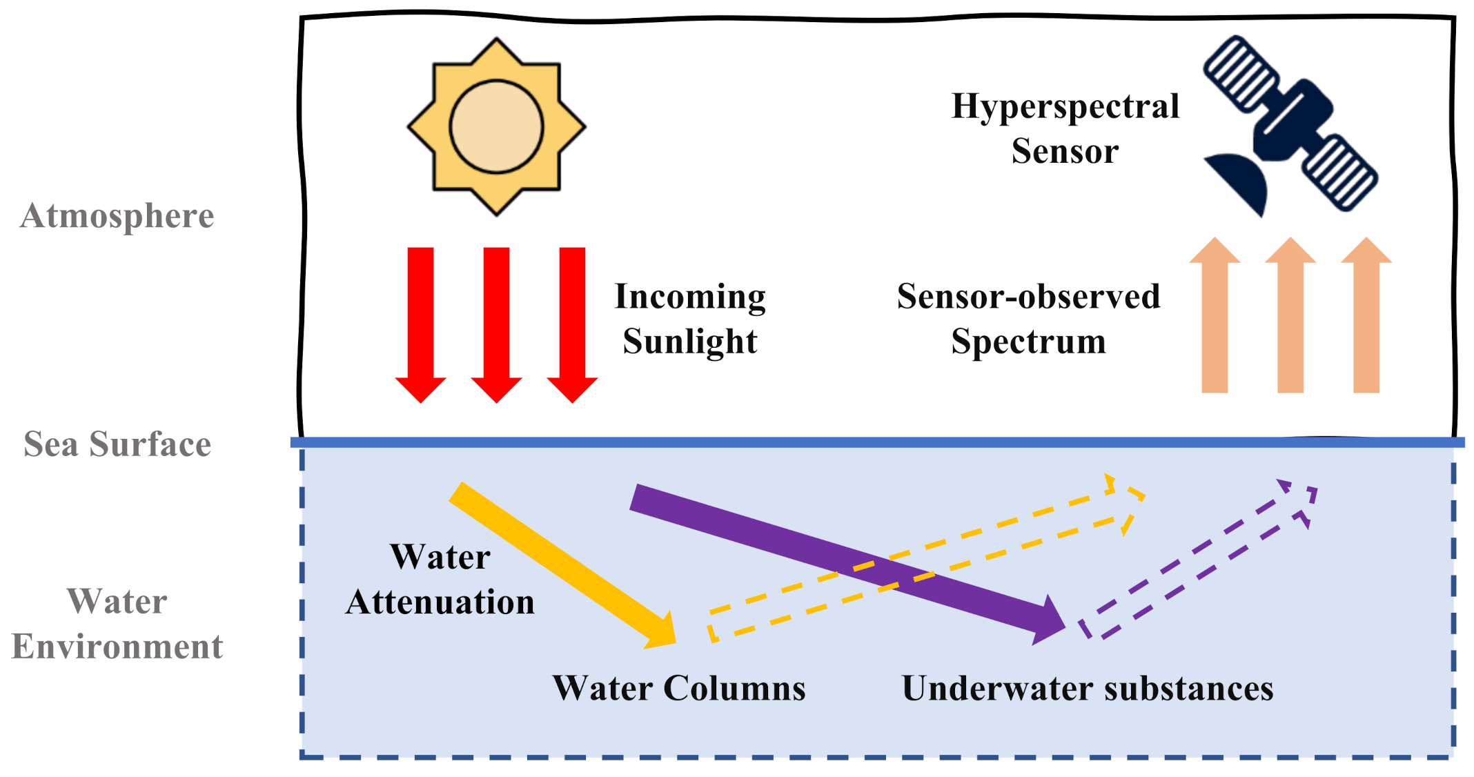
Generally speaking, the bathymetric model, depicting the generation process of sensor-observed spectrum in an underwater HSI, can be interpreted as a specific mathematical formula. Although intuitively, the aforementioned generation process can be illustrated in Figure 1. The sunlight firstly enters into the body of water and then is reflected by the water columns or targets of interest. During this transmission process, a considerable amount of attenuation will be imposed on the sunlight owing to the interference of the surrounding water. Therefore, the hyperspectral sensor would gather the reflectance spectra derived from water columns and the desired targets with the influence of water attenuation. More specifically, sensor-observed underwater spectrum represents a linear combination of two different kinds of reflectance spectra while the weight coefficients are determined by water attenuation [26]. Then, the general bathymetric model can be formulated as:

$$\mathbf{r}\left(\lambda \right)={\mathbf{r}}_{\infty }\left(\lambda \right)\left(1-{\mathrm{e}}^{-\left(k_d\left(\lambda \right)+k_u^c\left(\lambda \right)\right)H}\right)+\frac{{\mathbf{r}}_B\left(\lambda \right)}{\pi }{\mathrm{e}}^{-\left(k_d\left(\lambda \right)+k_u^b\left(\lambda \right)\right)H},$$

(1)

where $\mathbf{r}\left(\lambda \right)$ is the sensor-observed spectrum, ${\mathbf{r}}_{\infty }\left(\lambda \right)$ represents the reflectance spectra derived from water column, and ${\mathbf{r}}_B\left(\lambda \right)$ denotes the prior information of targets. $k_d\left(\lambda \right)$ refers to the attenuation coefficient associated with the downwelling procedure while $k_u^b\left(\lambda \right)$ and $k_u^c\left(\lambda \right)$ represent the attenuation coefficients of the upwelling procedure. H is the depth information of underwater water substance.

In Equation (1), ${\mathbf{r}}_{\infty }\left(\lambda \right)$ and ${\mathbf{r}}_B\left(\lambda \right)$ can be regarded as the prior knowledge but the rest of the parameters are required to be figured out before detection. Among all the unknown parameters, H is one of the most vital parameters which decides the water environment to “optical shallow” or “optical deep” [17]. When the location is too deep to permit any light from reaching the underwater substance, H will tend to be positive infinity and the bathymetric model is going to degrade as a target-free model:

$$\mathbf{r}\left(\lambda \right)={\mathbf{r}}_{\infty }\left(\lambda \right).$$

(2)

2.2. EM Theory

Obviously, a labeled dataset is necessary for training a deep neural network. Unfortunately, we can only collect the dataset with a fraction of labeled samples in practice. EM theory is one of the prevalent methods to tackle this dilemma by updating the network in an iteration scheme. The basic idea of this method in deep learning application is that labeled data can be employed to train a model, and then the trained model in turn assists to predict the labels of unlabeled data, while selecting the confident ones as new labeled training data, named pseudo-labeled data. Let L and U denote the labeled data and unlabeled data, and for a given network N, the EM method can be processed as follows:

• Step 1: Train N with L and then predict U with N;
• Step 2: Select some pseudo-labeled samples from U for which N has the highest confidence scores to construct a subset $\tilde{U}$$(\tilde{U}\subset U)$;
• Step 3: Remove $\tilde{U}$ from U and add $\tilde{U}$ into L for generating a novel training data $\tilde{L}$;
• Step 4: Repeat Steps $1\sim 3$ until the network converges.

In general, we denote the first step in the above process as $\mathbf{E}$ step, which figures out the optimal weight parameters for DNN based on a limited labeled dataset. The second and third steps will be merged into one step named the $\mathbf{M}$ step for dynamically yielding reliable pseudo-labeled data.

3. Proposed Method

In this section, we will minutely demonstrate the framework of our proposed method. So as to make full use of the prior knowledge of input HSI, a water IOPs retrieving method called IOPE-Net [27] is employed to estimate the water-associated parameters (all the unknown parameters except depth information) mentioned in Equation (1). This effective network develops a hybrid sequence structure to retrieve the water IOPs from water HSI in an unsupervised fashion and achieves an excellent estimation result. Therefore, in the remainder of this paper, we assume that the water-associated IOPs parameters have been well figured out by IOPE-Net beforehand, which can be considered as the prior information.

3.1. Self-Improving Underwater Target Detection Framework

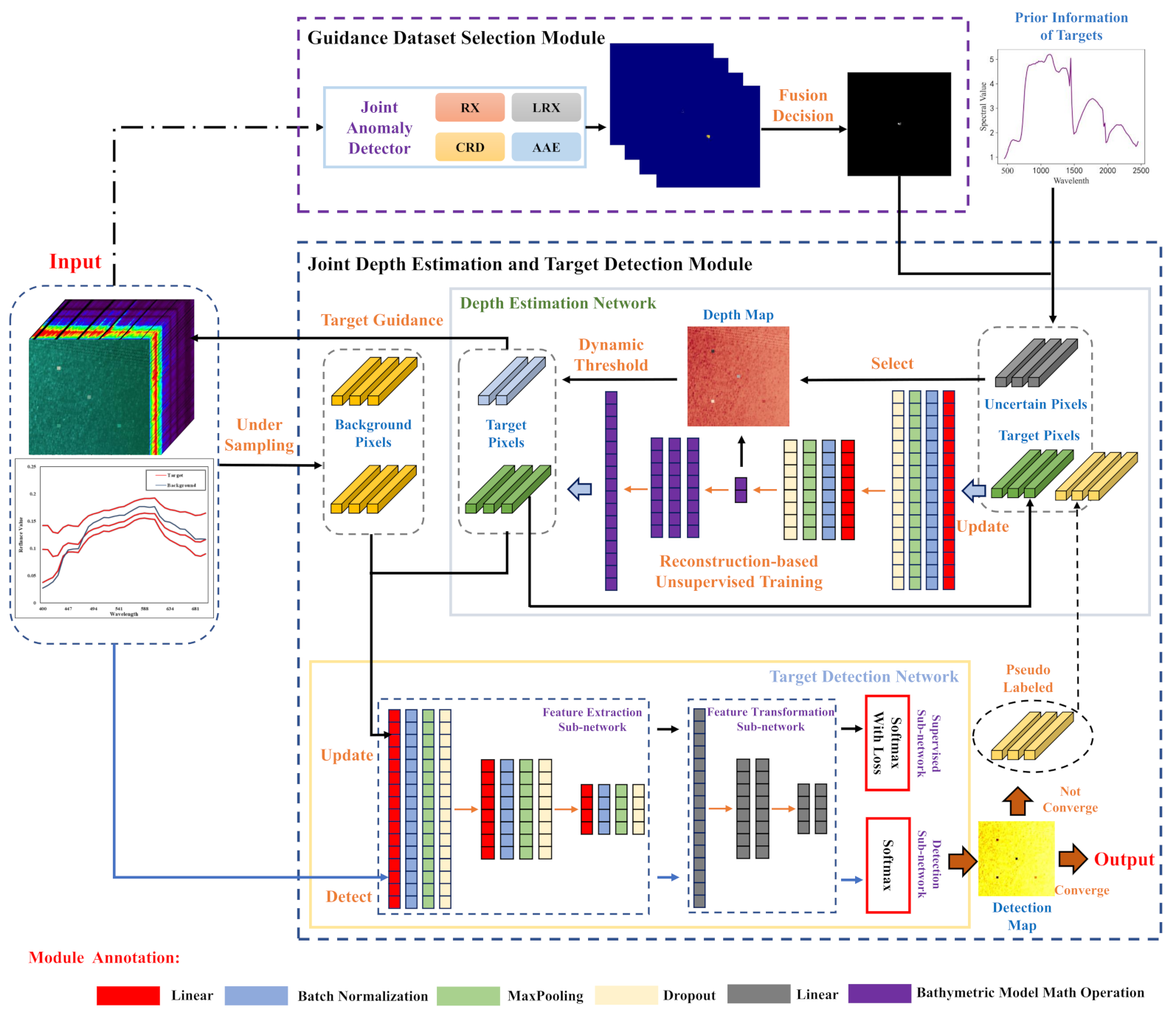
SUTDF is a general underwater detection framework managing to achieve a promising detection performance with depth information of desired targets. The depth information of underwater targets turns out to be a favorable metric for UTD which is position-sensitive and could contribute a lot to distinguishing the background and target pixels. Different from other existing methods, the proposed framework uses the spectral and spatial contextual information to establish the guidance dataset for activating the subsequent structures while alleviating the effect of lacking prior information. Then, deep learning methodologies are employed to jointly perform depth estimation and target detection in a data-driven method. However, due to the limitation of spectral and spatial contextual information, the depth estimation and target detection networks can merely achieve a partial solution. To tackle this issue, we propose an expectation maximization liked updating scheme which can make full use of the statistical and structural information of input HSI to literately update the depth estimation and target detection networks for attaining the more satisfied results. As illustrated in Figure 2, SUTDF consists of two modules: Guidance Dataset Selection Module and Joint Depth Estimation and Target Detection (JDETD) Module.

Guidance dataset selection module is the initial part of SUTDF, which devotes to creating the guidance dataset for the JDETD module. According to Figure 2, the depth estimation network requires to be trained with the pixels containing targets of interest. Owing to the limitation of the prior knowledge, it is hard to pick out these target-associated pixels from the input HSI directly. However, the target-associated pixels can be treated as outliers that can be detected by hyperspectral anomaly detection methods. Therefore, a specific joint anomaly detector is designed to find out outliers from the input HSI and we set a high threshold to select the pixels with high confidence coefficients for generating a guidance dataset. Note that, the high threshold improves the purity but decreases the completeness of the guidance dataset simultaneously.

The JDETD module, comprising a depth estimation network, a target detection network, and a specific self-improving iteration scheme, refers to the most vital part of SUTDF. The overall flow of this module can be depicted as follows. With the contribution of the guidance dataset, the depth estimation network is capable of generating the depth estimation map from the input HSI. Then, an under-sampling strategy is utilized to produce the training dataset for the target detection network and the detection map is available after the target detection network has been well-fitted. Considering the incompleteness of the guidance dataset, a self-improving iteration scheme is developed to update the parameters of the above two networks for achieving a more accurate detection result. During each iteration, the depth estimation map is employed to improve the capacity of the target detection network by enlarging the diversity of the training dataset, while the more accurate detection result will in turn promote the depth estimation performance via finding out more target-associated pixels. When the training datasets for these two networks no longer alter, the whole framework arrives to convergence stating that the information of the desired targets and water environment has been maximally utilized with little initial prior knowledge. Moreover, the JDETD module can use an underfitting depth estimation network to promote the detection performance by a particular joint performing manner rather than requiring the depth information to be well-estimated.

The concrete details of these two modules are exhibited in the following subsections.

3.2. Guidance Dataset Selection Module

As mentioned beforehand, we would utilize anomaly detection methods to select the target-associated pixels from input HSI. However, a single anomaly detection method would fail to make full use of the abundant spectral information, leading to a poor detection performance. To address this issue, the detection of target-associated pixels is performed by different typical anomaly detection methods and ensemble learning method. Primarily, we employ a set of typical anomaly detection methods to dispose the input HSI:

$${\mathbf{A}}^k=f^k\left(\mathbf{X}\right),k=1,2,\cdots ,K,$$

(3)

where $\mathbf{X}\in {\mathbb{R}}^{L\times B\times W}$ represents the input HSI, K is the amount of typical anomaly detection methods, and $f^k$ and $A^k\in {\mathbb{R}}^{L\times B}$ refer to the k-th anomaly detection method and its corresponding detection map. Considering the diversities of anomaly detection results, four typical anomaly detectors RX [28], LRX [29], CRD [30], and AAE [31] are employed as the anomaly detectors in this work. Then, the ensemble learning methodology is exploited to fuse all the detection maps for generating a stable and comprehensive result. The fusion strategy is based on weight voting theory and it can be demonstrated as follows:

$${\widehat{a}}_{i,j}=\frac{{\sum }_{m=1}^K{a}_{i,j}^m·g\left(a_{i,j}^m\right|\tau )}{K},$$

(4)

where ${\widehat{a}}_{i,j}$ and $a_{i,j}^m$ are the entries in the i-th row and j-th column of the fusion result and m-th anomaly detection result. $g\left(x\right|\tau )$ refers to threshold function, which is used to label the anomaly detection result:

$$g\left(x|\tau \right)=\left\{\begin{array}{cc}0,\hfill & x⩽\tau \hfill \\ 1,\hfill & x>\tau \hfill \end{array}\right.$$

(5)

where 0 refers to background pixels and 1 represents target-associated pixels. Note that, the mission of this joint anomaly detector is to select a few target-associated pixels rather than finding out all of them. Consequently, the hyperparameter $\tau$ in Equation (5) will be endowed with a large value for the sake of removing background pixels as much as possible. Besides, considering the scale discrepancy among the detection results of different anomaly detection methods, the normalization operation will be conducted before the fusion process.

3.3. Joint Depth Estimation and Target Detection Module

There is no doubt that the JDETD module plays the most crucial role in SUTDF. This specific module is made up of three components and the concrete information of these components is demonstrated in the remainder of this subsection.

3.3.1. Unsupervised Autoencoder-Form Network for Depth Estimation

As mentioned beforehand, the water-associated parameters have been computed by the IOPE-Net. That is, the bathymetric mentioned in Equation (1) will become a simple function with the only variable depth information H. Besides, the sensor-observed spectra are HSI and are also known as prior knowledge. Therefore, estimating the target depth information can be transformed into finding out the solution of a linear equation with a single variable. However, it is difficult to use typical mathematical convex optimization (MCO) methods to solve this linear equation. On the one hand, due to the redundant spectral information of input HSI, the rank of the coefficient matrix is smaller than the rank of augmented matrix for the above linear equation. Under this condition, MCO is not capable of finding out a real number solution. On the other hand, the impact of spectral variability derived from environment factors will make it difficult for MCO methods to acquire a stable result. Moreover, previous works [24,25] have confirmed that MCO is time-consuming, especially in dealing with large-scale datasets.

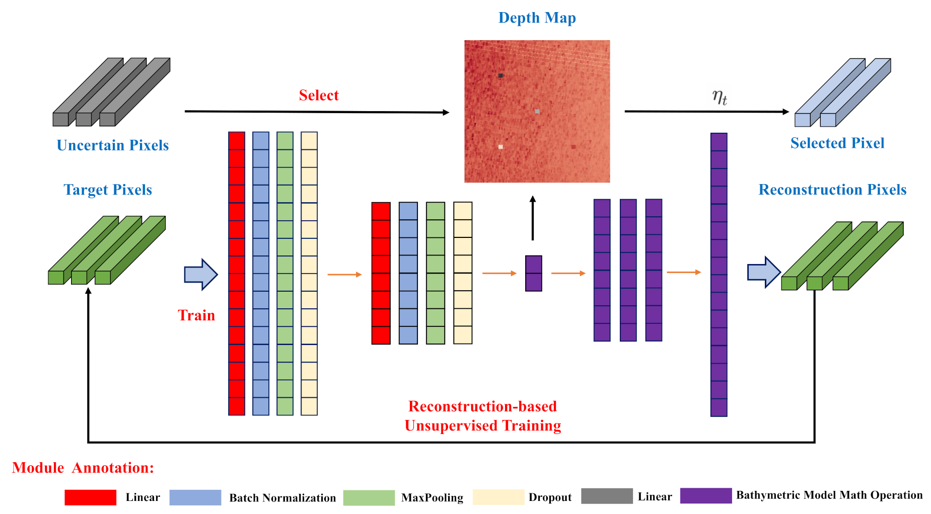
A deep neural network is one of the prevalent techniques solving optimization problems by learning the characteristic of datasets, which is deemed to attain the global optimal solution once the network has been well-fitted. Owing to being short of the ground-truth about depth information, in this paper we propose an autoencoder-form depth estimation network demonstrated in Figure 3. The structure of estimation network consists of two components, named the encoder and decoder.

The encoder part, possessing two independent blocks, acts as a predictor to estimate the depth information in this network. The first block is built with 1-D CNN, which devotes to attaining middle-level, locally invariant, and discriminative features from the input spectrum while eliminating the adverse impact of spectral variability. Given an input pixel $\mathbf{x}={\left\{x_i\right\}}_{i=1}^B\in {\mathbb{R}}^B$ with B bands, the output of t-th layer in the first block is defined as:

$${\mathbf{y}}^{\left(t\right)}=\left\{\begin{array}{cc}h\left({\mathbf{w}}^{\left(t\right)}\ast \mathbf{x}+{\mathbf{b}}^{\left(t\right)}\right),\hfill & t=1\hfill \\ h\left({\mathbf{w}}^{\left(t\right)}\ast {\mathbf{y}}^{(t-1)}+{\mathbf{b}}^{\left(t\right)}\right),\hfill & t\ge 2\hfill \end{array}\right.,$$

(6)

where ${\mathbf{w}}^{\left(t\right)}$ and ${\mathbf{b}}^{\left(t\right)}$ are weight parameters of the t-th layer, ∗ denotes the convolution operation, and h refers to the nonlinear activation function contributing to impose nonlinearity on the encoder network. In this work, ReLU [32] is exploited as the activation function, which has been widely used to tackle the gradient vanish issue. The batch normalization and dropout tricks are also applied to this CNN-based block for improving the speediness of convergence. The second block is composed with the fully connected layers. It can flatten the spectral features generated by the first block and use them to predict depth information.

Regarding the decoder part, it is utilized to reconstruct the input spectrum according to the predicted depth information. Unlike the traditional decoder, this network structure does not own any weight parameters and can be interrupted as a linear transformer to embed the bathymetric model into the depth estimation network. Several element-wise math operation layers are devised in the decoder part, which correspond to the bathymetric operation mentioned in Equation (1). After deposing by this specific decoder, we can attain the reconstruction spectrum $\widehat{\mathbf{x}}$ from the depth estimation result. Apart from the spectrum reconstruction function, this decoder part also makes the depth estimation network become model-driven and explainable. With the bathymetric model embedding operation, our method follows the same physical background as existing research works with the contribution of this specific decoder.

Obviously, the objective function is one of the most important factors for DNN, which teaches the network how to adjust its parameters. In this work, we use a multi-criterion reconstruction error containing three loss terms as the objective function. This particular objective function devotes to depicting the spectral discrepancy from different aspects.

(1) Mean Square Error Loss: The first term is calculated by the $l_2$ norm, which measures the spectral discrepancy with Euclidean distance:

$$L_{MSE}={\parallel \mathbf{x}-\widehat{\mathbf{x}}\parallel }_2,$$

(7)

where ${\parallel ·\parallel }_2$ is the $l_2$ norm of a given vector. Under the favorable derivative characteristic, this term is readily implemented by an existing deep learning framework (e.g., Pytorch).

(2) Spectral Angle Loss: The second item refers to the spectral angle loss between input spectrum $\mathbf{x}$ and reconstruction spectrum $\widehat{\mathbf{x}}$. This specific metric contributes to penalizing the spectral difference in the spectral shape aspect and its physical essence turns out to be the spectral angle between $\mathbf{x}$ and $\widehat{\mathbf{x}}$:

$$L_S=\frac{1}{\pi }arccos\frac{\mathbf{x}·\widehat{\mathbf{x}}}{{\parallel \mathbf{x}\parallel }_2{\parallel \widehat{\mathbf{x}}\parallel }_2}.$$

(8)

To unify the scales of different loss terms, we divide the spectral angle by a constant $\pi$ to map the value range $[0,1]$.

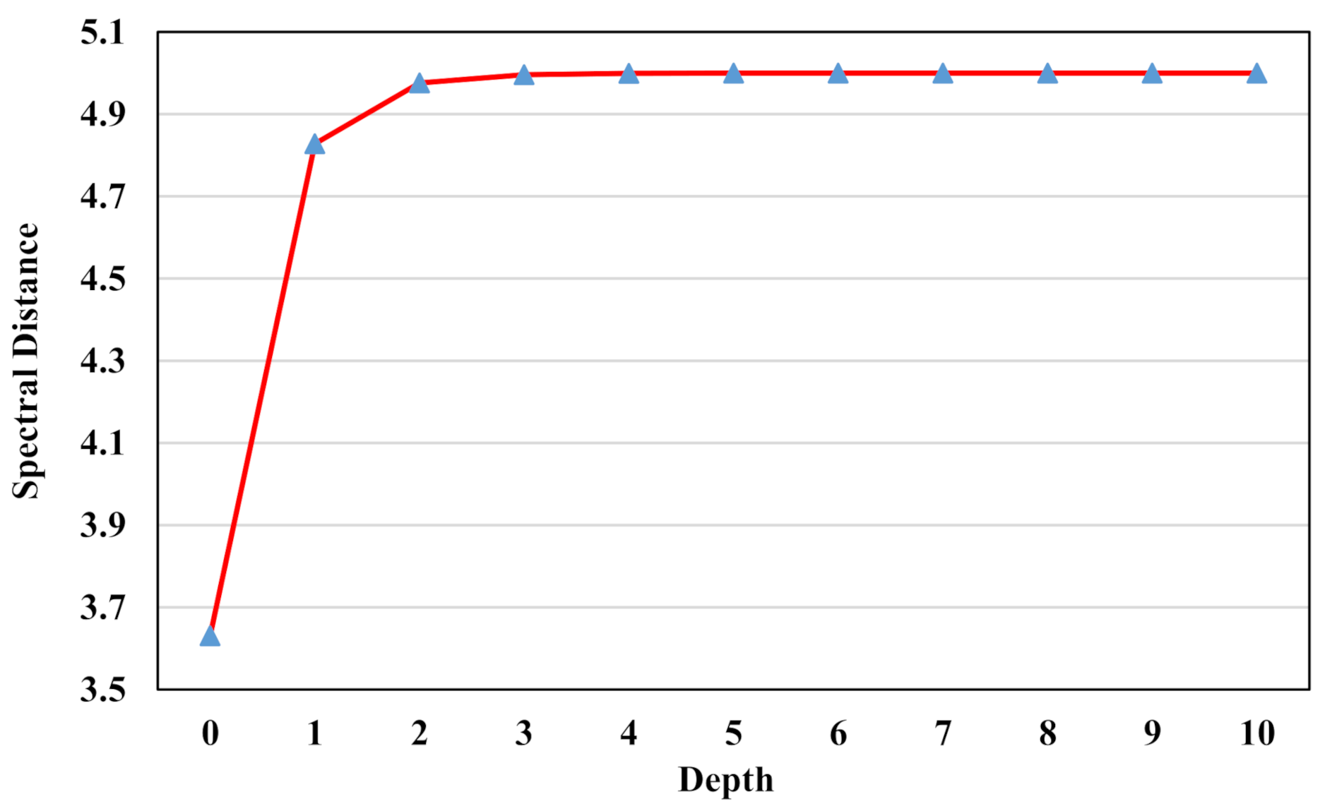
(3) Depth Value Constraint Loss: According to Figure 4, as the depth value increases, the spectral distance between sensor-observed spectrum $\mathbf{r}\left(\lambda \right)$ and land-based spectrum ${\mathbf{r}}_B\left(\lambda \right)$ is becoming larger. However, the degree of this change in spectral distance gradually decreases and finally turns into zero. In other words, when depth information exceeds a certain value, altering the depth value would not have the impact on $\mathbf{r}\left(\lambda \right)$. This phenomenon would lead to the gradient vanishing problem if the depth estimation network has not been well initialized and then predicts the depth information as a large value. The precondition of figuring out the depth information is that the target-associated spectrum should be distinguishable from the background spectrum. However, as the value of depth information increases, the target-associated pixel will finally turn into the background pixels. Therefore, the depth value constraint loss, which restricts depth information H to a relatively small value, is required for contributing to the convergence of the depth estimation network.

To put everything together, the depth estimation network will fit its weight parameters by the following multi-criterion objective function:

$$L=L_{MSE}+{\lambda }_s{L}_S+{\lambda }_H{\parallel H\parallel }_2$$

(9)

where ${\lambda }_s$ and ${\lambda }_H$ are hyperparameters representing the importance of $L_S$ and ${\parallel H\parallel }_2$ for the overall objective function. Both of these two parameters will be determined according to the training datasets.

Glancing over the depth estimation network, the decoder part contributes to predicting the depth estimation based on spectral characteristics and the objective function would teach the decoder part how to predict depth information more precisely. Due to this particular unsupervised training manner, we could acquire the depth information without any ground-truth information. Moreover, this manner simultaneously guarantees that when the input becomes a background pixel, noise point, or other target-associated pixel, the estimation result will turn into a relatively large value which can be regarded as an outlier in a depth map. It will help to eliminate the interference of environment factors and then a more satisfied depth estimation performance is achievable for a given HSI dataset.

3.3.2. Binary Classifier Network for Target Detection

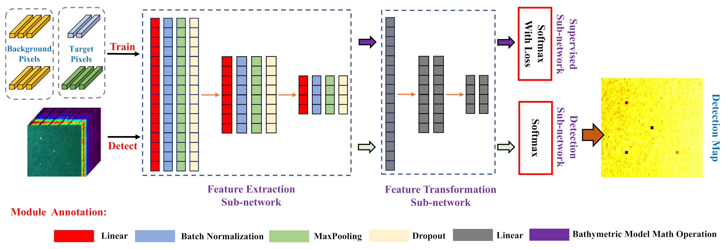
Underwater target detection can be implicitly explained as a binary classifier whose assignment is categorizing all the pixels into a target group or background group. Furthermore, the classification map and detection map have an identical physical essence which are both used to represent a confidence coefficient of being the target or background for each pixel. Consequently, we design a binary classifier based on deep learning methodology to finish the underwater target detection task. As illustrated in Figure 5, this particular target detection network is comprised of four subnetworks: Feature extraction sub-network, feature transform sub-network, supervised training sub-network, and detection sub-network.

Feature extraction sub-network. The feature extraction is a stack of cascade DNN blocks with different convolution steps. Here, in each block, there exists a convolution layer, pooling layer, batch normalization, dropout, and nonlinear activation. Similar with the first block in the encoder part, we employ this sub-network to refine the spectral information provided with input HSI. Besides, it can also assist to reduce the network parameters, adapt the spectral variability, and boost the generalization ability for the target detection network.

Feature transformation sub-network. The feature transformation sub-network is made up of some fully connected layers containing different amounts of neurons, which is utilized to predict the class probability for each pixel. This sub-network firstly flattens the spectral features derived from the last sub-network for dimensionality reduction. Then, it transforms the flattened feature vector into a two-dimensional prediction vector. To make the sub-network more capable and stable, the nonlinear activation function and dropout trick are also imposed between different fully connected layer blocks.

Supervised training sub-network. The proposed DNN-based binary classifier requires to be trained in a supervised fashion. With the assistance of a depth estimation network, we are capable of determining which pixels contain targets of interest. However, these pixels only occupy a tiny percent of the total HSI, resulting in a class imbalance problem. To address this problem, we adopt an under-sampling strategy to pick out a suitable training dataset at the very beginning. After that, a softmax function is exploited to transform the prediction vector yielded by feature transformation sub-network into a probability distribution over different classes. Then, the supervised training sub-network computes the logistic loss between the predict vector and the one-hot vector of training labels to be the objective function. Finally, the depth estimation network is trained with the calculated logistic loss and the stochastic gradient descent algorithm.

Detection sub-network. The detection sub-network is the final component of the target detection network and it is exploited to determinate the category for each testing pixel. Analogously, the detection sub-network only contains a softmax function. However, compared with a supervised training sub-network, all the pixels of input HSI are fed into this subnetwork to predict their categorical attributes, finally generating the detection map. For the sake of attaining a confident detection result, a labeling strategy based on maximum a posteriori probability criterion is proposed as follows:

$$l=\underset{i}{argmax}p(y=i\mid \mathbf{x},N),i=0,1,$$

(10)

where $\mathbf{x}$ is the input pixels and N refers to the target detection network. $p(y=i\mid \mathbf{x},N)$ represents the posteriori probability of class label i with a determinate input pixel $\mathbf{x}$ and network N. This detection sub-network actually conducts the testing process to encode the input HSI into a detection map consisting of numerous one-hot probability vectors.

3.3.3. Self-Improving Iteration Scheme

Under an ideal condition, we would manage to perform the underwater target detection with aforementioned two networks. Unfortunately, the joint anomaly detector can not find out all the target-associated pixels with little prior information. Then, the depth estimation network and target detection network will not be well fitted on account of training with biased datasets. As a result, our proposed method can only provide a suboptimal solution for the underwater target detection problem. In order to tackle this dilemma, we decide to perform the joint depth estimation and underwater target detection with a self-improving iteration scheme.

Different from other machine learning methods, DNNs possess a promising generalization capability so that the networks can achieve the correct results even if the inputs are not contained in training dataset. Consequently, the testing result can be used to boost the network with some specific principles [33]. However, if we employ the testing result of one DNN to improve itself, the iteration process would be sensitive to bad examples and finally crash owing to error accumulation. Therefore, in this work, we employ a depth estimation network and detection network to alternately boost the entire detection performance. Furthermore, there is no doubt that the generalization ability of a DNN is limited but we can eliminate this limitation by designing an updating scheme for the whole network based on the EM theory. In this way, we propose a self-improving iteration scheme which contributes to improving the performance of joint depth estimation and underwater target detection simultaneously by utilizing the training experience accumulation. Motivated by above perspectives, the self-improving iteration scheme is conducted as follows.

At the very beginning, input HSI is divided into two groups: Target-associated pixels set $T_0$ and uncertain pixels set $U_0$. We first consider the initial depth estimation network $E_0$ that is trained over the limited dataset $T_0$. According to the analysis mentioned above, it is achievable to label the uncertain pixels based on the depth estimation result. Compared with background pixels, the depth information of target-associated pixels possess two unique characters: (1) Their values are relatively small and (2) they occupy a small percentage. Consequently, we select the pixels with depth values less than a certain threshold ${\eta }_t$ to label as targets. As for the threshold ${\eta }_t$, it is associated with the capability of depth estimation network. With the training experience accumulating, the network will perform better in depth estimation and then we can figure out the depth information of targets locating in deeper positions. In this way, we need to dynamically increase the value of threshold ${\eta }_t$ during the updating process. Therefore, a time-varying threshold is proposed to fit this specific requirement:

$${\eta }_t={\eta }_{\infty }·(1-e^{-\gamma t}),$$

(11)

where ${\eta }_{\infty }$ refers to the largest value of the threshold ${\eta }_t$, t denotes as the number of iterations, and $\gamma$ is the hyperparameter to control the growth rate. Then, we can pick out a target-associated pixel subset $U^{{}^{\prime }}$ from the uncertain pixels set $U_0$ by:

$$U^{{}^{\prime }}=\left\{\mathbf{x}\right|E_0\left(\mathbf{x}\right)\le {\eta }_0,\mathbf{x}\in U_0\},$$

(12)

where $E_0\left(\mathbf{x}\right)$ represents the depth information calculated by the depth estimation network $E_0$ for an uncertain pixel $\mathbf{x}$.

In the following, the subset $U^{{}^{\prime }}$ is exploited to generate the novel target-associated pixels set $T_0^{{}^{\prime }}$$(T_0^{{}^{\prime }}=U^{{}^{\prime }}\cup T_0)$ and uncertain pixels set $U_0^{{}^{\prime }}$$(U_0^{{}^{\prime }}=U_0-U^{{}^{\prime }})$. Meanwhile, we can acquire the training data $D_0$ for initial target detection network $C_0$ with the under-sampling strategy (randomly sample a pixel subset with the same sample capacity as $T_0^{{}^{\prime }}$ from $U_0^{{}^{\prime }}$ to be background pixels). Using the dataset $D_0$, we update the target detection network $C_0$ and select a new subset of target-associated pixels $U^{{}^{″}}$ according to the following calculation:

$$U^{{}^{″}}=\left\{\mathbf{x}\right|p\left(y=target\mid \mathbf{x},C_0\right)>1-{\eta }_0,\mathbf{x}\in U_0^{{}^{\prime }}\},$$

(13)

where $p\left(y=target\mid \mathbf{x},C_0\right)>1-{\eta }_0$ represents the probability of being a target-associated pixel calculated by the target detection network $C_0$ for an uncertain pixel $\mathbf{x}$. In the same way, the new target-associated set $T_1$$(T_1=T_0^{{}^{\prime }}\cup U^{{}^{″}})$ and uncertain pixel set $U_1$$(U_1=U_0^{{}^{\prime }}-U^{{}^{″}})$ are available and they will be utilized to update the depth estimation network $E_1$. We would repeat this process until the performances of the depth estimation network and target detection network do not improve any more.

In summary, the total process of the proposed framework is shown in Algorithm 1. It is noticeable that we employ the network parameters derived from the penultimate training epoch instead of the last one since the network parameters in last training epoch have been overfitting.

Algorithm 1 The total process of the proposed framework.

Input: HSI $\mathbf{X}$, anomaly detection methods set ${\left\{f^i\right\}}_{i=1}^K$, hyperparameters $\tau$, $\gamma$ and ${\eta }_{\infty }$ Output: Underwater target detection map and depth map.   1: for$i=1,2,\cdots ,K$do   2:     Compute the result $A^k$ with k-th anomaly detector according to Equation (3);   3: end for   4: Figure out joint anomaly detection result by Equation (4);   5: Construct target-associated pixels set $T_0$ and uncertain pixels set $U_0$ according to threshold $\tau$;   6: Initialize a depth estimation network $E_0$;   7: Initialize a target detection network $C_0$;   8: $i\leftarrow 0$;   9: while$E_i$ and $C_i$ do not converge do 10:     Calculate the dynamic threshold ${\eta }_i$ by Equation (11); 11:     Train $E_i$ with $T_i$; 12:     Generate a target-pixels subset $U^{{}^{\prime }}$ from $U_i$ based on: $$U^{{}^{\prime }}=\left\{\mathbf{x}\right|E_i\left(\mathbf{x}\right)\le {\eta }_i,\mathbf{x}\in U_i\};$$ 13:     Update $T_i^{{}^{\prime }}\leftarrow T_i\cup U^{{}^{\prime }}$; 14:     Update $U_i^{{}^{\prime }}\leftarrow U_i-U^{{}^{\prime }}$; 15:     Establish training data $D_i$ by under-sampling from $U_i^{{}^{\prime }}$ according to $T_i^{{}^{\prime }}$; 16:     Train $C_i$ with $D_i$ ; 17:     Generate a target-pixels subset $U^{{}^{″}}$ from $U_i^{{}^{\prime }}$ based on: $$U^{{}^{″}}=\left\{\mathbf{x}\right|p\left(y=target\mid \mathbf{x},C_i\right)>1-{\eta }_i,\mathbf{x}\in U_i^{{}^{\prime }}\};$$ 18:     Update $T_{i+1}\leftarrow T_i^{{}^{\prime }}\cup U^{{}^{″}}$; 19:     Update $U_{i+1}\leftarrow U_i^{{}^{\prime }}-U^{{}^{″}}$; 20:     $i\leftarrow i+1$; 21: end while 22: Calculate the depth map by feeding $\mathbf{x}$ into $E_{i-1}$; 23: Figure out the detection map by feeding $\mathbf{x}$ into $C_{i-1}$;

4. Experiments

In this section, expensive experiments have been performed on different underwater datasets to evaluate the performance of SUTDF. First of all, we briefly introduce the necessary information about the employed datasets. Secondly, subsection Experiment Details lists the employed evaluation criteria and parameters settings for all the experiments. Then, two specific experiments are designed to validate the effectiveness of the innovativeness proposed in Section 3. After that, we describe the underwater detection experiments and their correspond discussions in detail. Finally, to comprehensively demonstrate our proposed methods, several tests for method analysis are conducted in the rest of this section.

4.1. Dataset Description

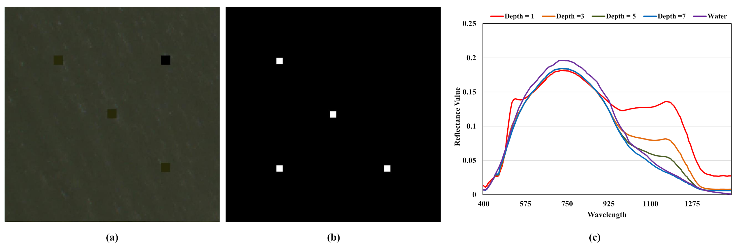
In an ideal situation, all the experiments could be performed on real datasets. Unfortunately, due to the novelty of a hyperspectral underwater target detection topic, there are no public hyperspectral datasets containing underwater targets. To tackle this issue, four synthetic HSI datasets generated by the scheme mentioned in [17] are employed in our experiments, which represent some specific targets locating in four different underwater scenarios. As for the amount of objects in each dataset, we employ the spectra of one material with four different depth information as the desired targets. Therefore, it can be regarded that four different objects are contained in each dataset. The dataset generation scheme can be summarized into the following seven steps:

• Step 1: Select a real-world underwater HSI as the background.
• Step 2: Calculate the mean vector of this HSI as the reflectance vector of water column background pixel ${\mathbf{r}}_{\infty }\left(\lambda \right)$.
• Step 3: Employ the IOPE-Net to retrieve the IOPs parameters $k_d\left(\lambda \right)$, $k_u^c\left(\lambda \right)$, and $k_u^b\left(\lambda \right)$ from underwater HSI.
• Step 4: Choose several spectra of different materials from USGS spectral library [34] as targets of interest ${\mathbf{r}}_B\left(\lambda \right)$.
• Step 5: Exploit background pixel ${\mathbf{r}}_{\infty }\left(\lambda \right)$, IOPs parameters $k_d\left(\lambda \right)$, $k_u^c\left(\lambda \right)$, $k_u^b\left(\lambda \right)$, and target spectra ${\mathbf{r}}_B\left(\lambda \right)$ to figure out the corresponding underwater target spectra $\mathbf{r}\left(\lambda \right)$ with different depth values H by Equation (1).
• Step 6: Impose the intra-class variability on the generated underwater target spectra by adding Gaussian noise with mean vector $\mu$ and covariance matrix $\sigma$ as follows:

  $$\widehat{\mathbf{r}}\left(\lambda \right)=\mathbf{r}\left(\lambda \right)+=\frac{1}{\sqrt{2\pi }\sigma }exp\left(-\frac{{(\lambda -\mu )}^2}{2{\sigma }^2}\right).$$

  (14)
• Step 7: Embed the noisy underwater target spectra $\widehat{\mathbf{r}}\left(\lambda \right)$ into real-world underwater hyperspectral image at different spatial positions by replacing the pixels there.

(1) Synthetic Data Based on Simulated Turbid Water: The first synthetic dataset is constructed with a simulated turbid water HSI whose water IOPs are provided by [22]. Meanwhile, the sheet metal material is appointed to be the targets of interest. The spatial solution of this dataset is $100\times 100$ and it possesses 150 bands covering from 400 nm to 700 nm. In terms of the depth values, we place the noisy underwater targets at 0.1 m, 1 m, 2 m, and 3 m concurrently. The detailed information of this dataset has been illustrated in Figure 6.

(2) Synthetic Data Based on Sea Water: The second synthetic dataset consists of hyperspectral sea water image and reflectance spectra of alunite material. This HSI is captured by Airborne Visible Infrared Imaging Spectrometer (AVIRIS) at a gullet locating in Galveston Bay, Texas, whose wavelength ranges from 366 nm to 2495 nm at 9.5 nm spectral solution. To further accomplish our experiments, an image chip with $384\times 384$ spatial solution was segmented out. Besides, we set the depth values of underwater targets as 0.5 m, 1 m, 2.5 m, and 5 m. Similarly, we demonstrate the concrete information about the second data in Figure 7.

(3) Synthetic Data Based on Lake Water: The background of the third synthetic dataset is collect by Gaofen-5 satellite with Advanced Hyperspectral Imagery (AHSI) in 2020. And the collection position is a scenario of Dongting Lake in Yueyang City, Hunan Province, China. This specific hyperspectral lake image has 330 spectral bands covering from 400 nm to 2500 nm and we select a $60\times 60$ chip as the experimental dataset. Furthermore, the spectra of particle board material are collected as the desired targets which are placed at the range of 0.1 to 5 m with an alterable step size. Figure 8 is exploited to exhibit the specific information of this dataset.

(4) Synthetic Data Based on River Water: The last synthetic dataset is derived from a hyperspectral river image and the spectra of nylon webbing material. This hyperspectral river image depicts the underwater scenario of Nangang River positioning in Guangzhou City, Guangdong Province, China. Unlike the other two real-world HSIs, this image has a more narrow spectral range from 400 nm to 1000 nm with a 2.22 nm spectral solution. Furthermore, considering the turbidity of this water scenario, the nylon webbing material is set as relevantly deep depths at 1 m, 3 m, 5 m, and 7 m. We segment out a experimental chip with $180\times 180$ pixels as illustrated in Figure 9 with the minute information of the last dataset.

To summarize, detailed information of all the experimental datasets are listed in

Table 1. The summary of the important information for all experimental datasets.

Dataset	Spatial Solution	Band Numbers	Target Material	Depth Information
Simulated water	$100\times 100$	150	Sheet metal material	0.1 m, 1 m, 2 m, and 3 m
Sea water	$384\times 384$	224	Alunite material	0.5 m, 1 m, 2.5 m, and 5 m
Lake water	$60\times 60$	330	Particle board material	0.1 m, 1 m, 2 m, and 5 m
River water	$180\times 180$	270	Nylon webbing material	1 m, 3 m, 5 m, and 7 m

in numerical form. For simplicity, we abbreviate the names of these datasets to “simulated water”, “sea water”, “lake water”, and “river water”.

4.2. Experimental Details

In order to further describe the experiment results for our research work, we will introduce the necessary experimental details in this section. Primarily, the evaluation criteria employed to measure the performance of testing methods are presented at the very beginning. Then, the remainder of this section shortly lists the experimental settings for all the datasets.

(1) Evaluation Criteria: To evaluate the performance of testing methods qualitatively, the receiver operating characteristic (ROC) curve is employed as a criterion. It is widely acknowledged that ROC is the most commonly used metric in computer vision tasks, which is presented to illustrate the correlation between false alarm rate (FAR) $P_f$ and target detection probability $P_d$ [35]. Moreover, the FAR $P_f$ reflects the percentage of falsely-detected pixels for the whole image:

$$p_f=\frac{N_f}{N}$$

(15)

where $N_f$ is the amount of falsely-detected pixels and N denotes the total number of pixels in the image. Meanwhile, the target detection probability $P_d$ refers to the ratio between correctly-detected pixels and target pixels among the entire image:

$$P_d=\frac{N_c}{N_t}$$

(16)

where $N_c$ is the number of correctly-detected pixels and $N_t$ represents the amount of target pixels in the whole image. Note that the methods, having the ROC curve locating near the top left of the coordinate plane, would exhibit a better detection performance in the associated detecting tasks. Besides, the area under ROC curve (AUC) values have also been figured out to attain a quantitative analysis about the detection result.

(2) Experimental settings: Threshold $\tau$, threshold ${\eta }_{\infty }$, and growth speed control factor $\gamma$ are important hyperparameters for our experiments. The specific values of these parameters for different datasets are listed in

Table 2. The hyperparameters settings for different datasets.

Parameter Name	Simulated Water	Sea Water	River Water	Lake Water
Threshold $\tau$	0.25	0.20	0.15	0.15
Threshold ${\eta }_{\infty }$	0.3	0.35	0.3	0.2
Growth speed control factor $\gamma$	0.1	0.2	0.1	0.05

. To construct the joint anomaly detector, typical anomaly detectors RX, LRX, CRD, and AAE are selected as the fundamental factors. Moreover, so as to further demonstrate the outperformance of the proposed method, the following methods are exploited to make a comprehensive comparison with the proposed method: (1) UTDF [17]; (2) GBF [18]; (3) CEM [36]; and (4) MF [37]. For all the testing methods, the input HSIs will be disposed by the ATCOR model [38] for removing the interference of the atmosphere. In addition, identical spectra of different materials are used as the prior target spectral information. Finally, the accomplishments of our experiments are supported by an Intel(R) Core (TM) i9-10920X CPU machine and 64 GB of RAM on Windows 10 operating system (Microsoft, Redmond, American), while the related codes are written with the assistance of the deep learning framework Pytorch 1.7.0 (Facebook, Menlo Park, American).

4.3. Component Analysis

In this section, some particular tests are designed to confirm the validation of the viewpoints we put forward in Section 3.

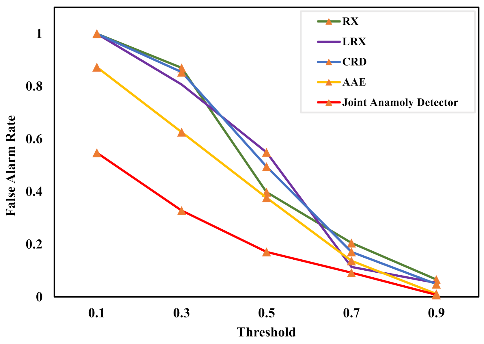
(1) Effectiveness Evaluation of the Joint Anomaly Detector: In Section 3.2, we have proposed a special joint anomaly detector which is assigned to select the target-associated pixels. To verify whether this detector is capable of further finding out the target-associated pixels, we employ four classical anomaly detection methods RX, LRX, CRD, and AAE to make a comparison. The mission of joint anomaly detector is picking out a pixel subset only containing target-associated pixels. Consequently, we calculate the FARs of the detection results under different thresholds as the comparison metric. For convenience, we merely perform this test on the first synthetic dataset and the calculation results are exhibited in Figure 10 and

Table 3. The FPR values of different methods with some certain thresholds for effectiveness evaluation of joint anomaly detector.

Threshold Value	False Alarm Rate Values
	RX	LRX	CRD	AEE	Joint Anamoly Detector
0.1	1	1	1	0.873	0.548
0.3	0.87	0.807	0.845	0.626	0.328
0.5	0.398	0.549	0.495	0.377	0.171
0.7	0.205	0.114	0.171	0.137	0.092
0.9	0.066	0.053	0.049	0.012	0.008

The bold entries represent the best performance in each row.

. Obviously, the joint anomaly detector has achieved the lowest FARs under all the given thresholds. Besides, this detector can achieve a satisfying FAR even if the threshold has been set as a small value. These phenomena indicate that the proposed anomaly detector can better eliminate the inference of background and attains a target-associated pixels selection result containing less background pixels which is more suitable for generating the guidance dataset.

(2) Effectiveness Evaluation of the depth value constraint on objective function: As mentioned in Equation (9), a depth value constraint has been imposed on the objective function. For the purpose of justifying whether depth value constraint has contributed to the training process and final detection result, SUTDF without this specific constraint has also been conducted on all the datasets. The training time and the AUC values of the detection result are exploited as the criteria, which are demonstrated in

Table 4. The AUC values and training time for effectiveness evaluation of depth values constraint.

Dataset	AUC Values		Training Time (in Seconds)
	SUTDF (Y)	SUTDF (N)	SUTDF (Y)	SUTDF (N)
Simulated water	0.92	0.84	36.308	58.471
Sea water	0.97	0.87	124.998	166.387
River water	0.91	0.78	72.686	104.748
Lake water	0.98	0.86	27.568	44.179
Average	0.945	0.8375	65.389	93.446

The bold entries represent the best performance in each row.

. We use characters Y and N (placed in parentheses) to present if the SUTDF has been trained with depth value constraint.

According to the last two columns of Table 4, it is effortless to find out the proposed method with the depth value constraint requiring less training time. This result implies that the depth value constraint will contribute to the speediness of network convergence. The intuitive reason accounting for this phenomenon is that depth value constraint will assist the gradient descent algorithm when it meets the stationary points or local optimal points during the training process. As for the detection result, the depth value constraint also significantly improves the detection performance containing a higher detection rate and a lower FAR.

4.4. Underwater Detection Performance

In this section, we will exhibit the underwater detection performance derived from all the datasets. As mentioned beforehand, two typical land-based target detection methods CEM and MF are exploited as the baselines for the methods comparison. In addition, two prevalent underwater detection methods have also been conducted to demonstrate a more comprehensive comparison result.

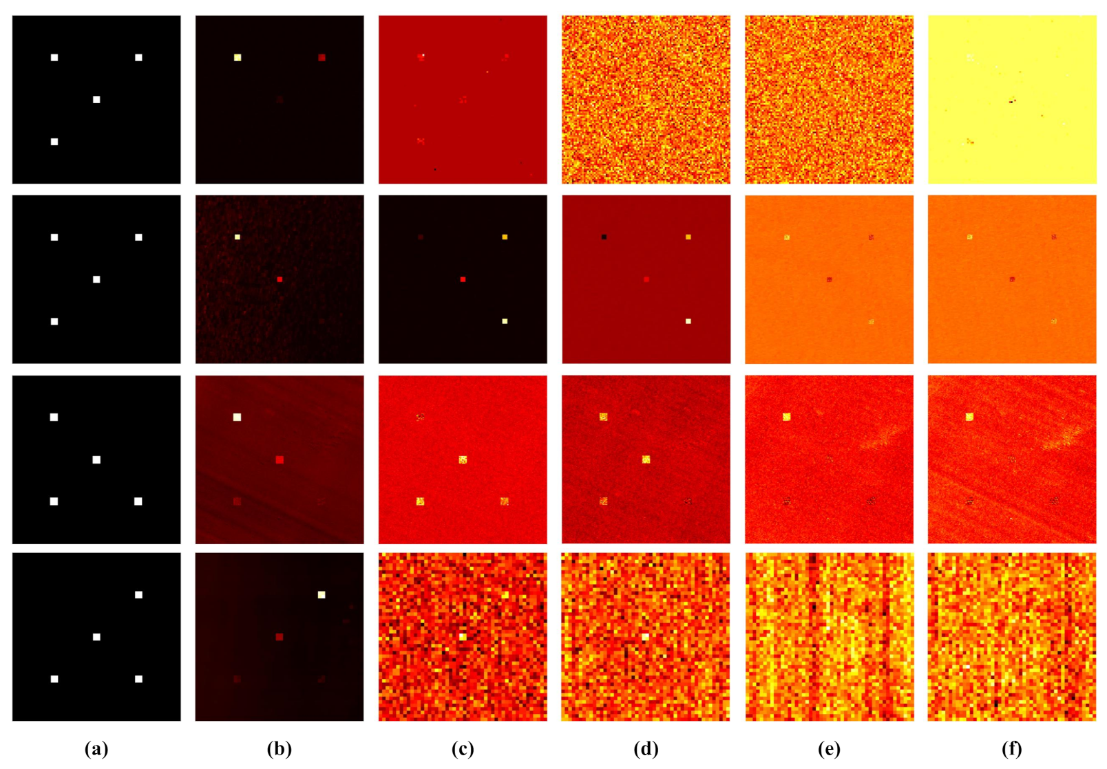
First of all, we will show the detection performance from a visual aspect. Figure 11 has demonstrated reference maps (such as ground truths and underwater detection maps) for all the datasets. The SUTDF achieved the slightest visual discrepancy with ground truths according to the visual judgement. Moreover, compared with other methods, SUTDF managed to eliminate the adverse influence of background pixels, where the fewest background pixels have been falsely detected in the detection maps. However, the typical land-based target detection methods performed badly in all the datasets, which confirms that the target background independent assumption no longer makes sense in underwater scenarios. As illustrated in Figure 11b, the proposed method is capable of attaining satisfied detection results even if the targets locate in relatively deep positions. This indicates that SUTDF possesses a stronger capacity in detecting dim and weak targets, which will contribute to broadening the application range of this specific framework in practice.

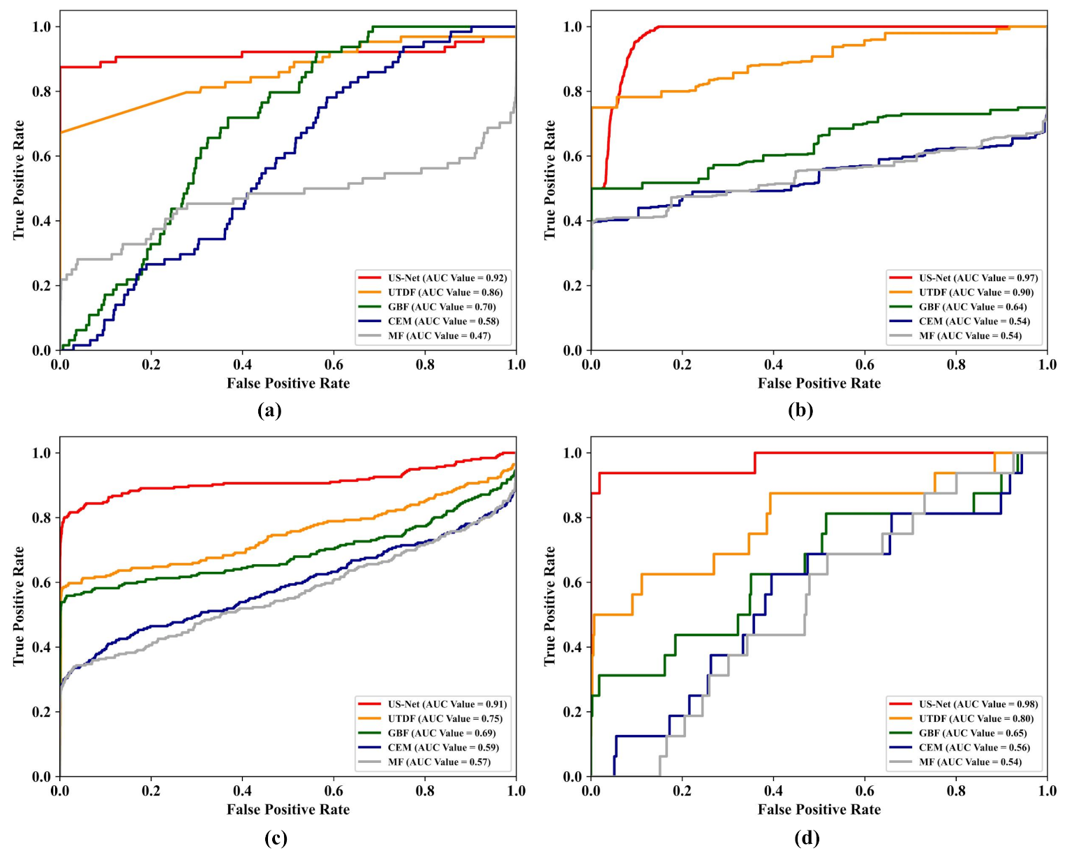
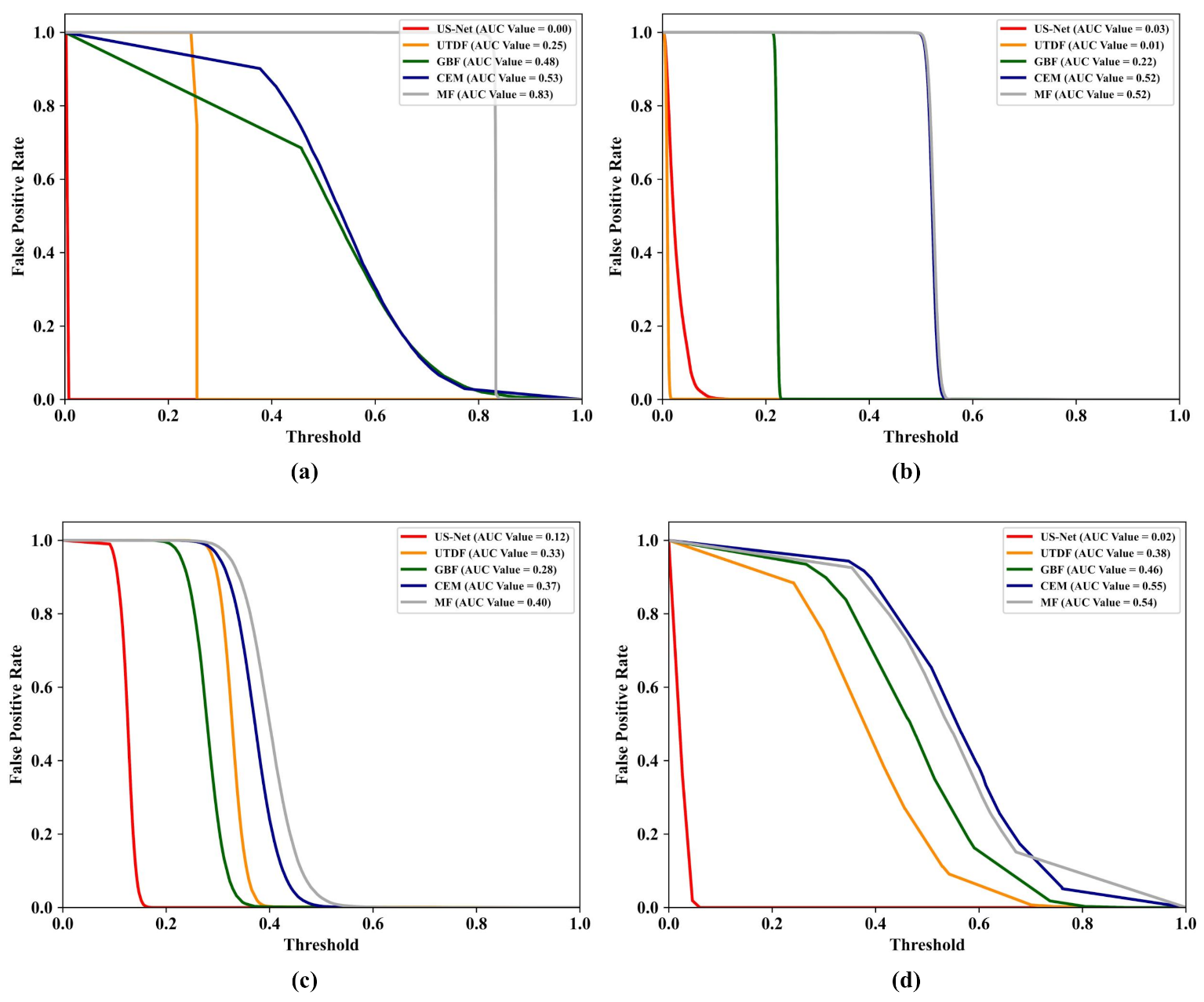
So as to conduct the qualitative analysis of the detection results, the ROC curves of $(P_D,P_F)$ and $(P_D,Threshold)$ have been plotted as another two critical comparison metrics. According to Figure 12, the ROC curves of $(P_D,P_F)$ of our method remains over other curves in all the experimental datasets except for the simulated water dataset. Moreover, the ROC curves of $(P_F,Threshold)$ of the SUTDF located at the bottoms of other compared methods for each dataset except the sea water dataset in Figure 13. Based on these two evidences, we could conclude that SUTDF creates a superior detection performance with the lower FARs.

For a quantitative comparison, the AUC values of $(P_D,P_F)$ and $(P_F,Threshold)$ are also calculated in this subsection. As listed in

Table 5. The AUC values of $(P_D,P_F)$ of underwater target detection results for compared methods on all datasets.

Dataset	Area Under ROC Curves of $({\mathit{P}}_{\mathit{D}},{\mathit{P}}_{\mathit{F}})$
	CEM	MF	GBF	UTDF	UTD-Net
Simulated water	0.47	0.58	0.70	0.86	0.92
Sea water	0.54	0.54	0.64	0.90	0.97
River water	0.57	0.59	0.69	0.75	0.91
Lake water	0.54	0.56	0.65	0.80	0.98
Average	0.53	0.5675	0.67	0.8275	0.945

The bold entries represent the best performance in each row.

, the AUC values of SUTDF are higher than other detection methods and all exceed 0.9. Especially in the lake water dataset, the proposed method achieves a AUC score of 0.98, which is appropriate to the optimal result. Furthermore, the average AUC value of $(P_D,P_F)$ of our method is 0.945 while the performance of the suboptimal detection method is only 0.8275. The statistical information in Table 5 further verifies that SUTDF yields the optimum detection results among all the compared detection methods. In terms of the FARs of the compared methods, the detailed information is listed in

Table 6. The AUC values of $(P_F,Treshold)$ of underwater target detection results for compared methods on all datasets.

Dataset	Area Under ROC Curves of $({\mathit{P}}_{\mathit{F}},\mathbf{Threshold})$
	CEM	MF	GBF	UTDF	UTD-Net
Simulated water	0.83	0.53	0.48	0.25	0.00
Sea water	0.52	0.52	0.22	0.01	0.03
River water	0.40	0.37	0.28	0.33	0.12
Lake water	0.54	0.55	0.46	0.38	0.02
Average	0.5725	0.4925	0.36	0.2425	0.0445

The bold entries represent the best performance in each row.

. Notably, compared with all the testing methods, SUTDF has achieved the best performance in FAR, although it fails to achieve the optimal result in the sea water dataset. The AUC value of $(P_F,Threshold)$ of our method is larger than the UTDF method in the sea water dataset, while the performance gap is 0.02 and can be ignored in practical application. However, in other experimental datasets, the proposed method attains the lowest FAR and the corresponding AUC values of $(P_F,Threshold)$ are all under 0.12. The average value of $(P_F,Threshold)$ of SUTDF is 0.0445 which confirms that SUTDF has successfully eliminated the interference of background pixels, leading to the global lowest FAR.

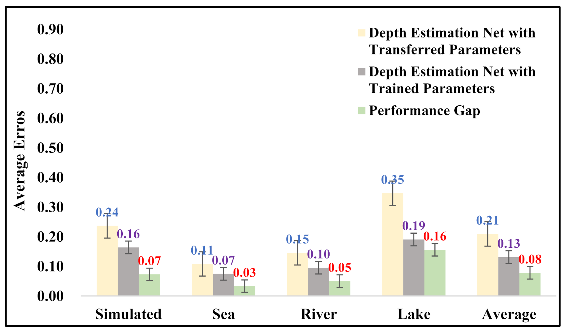
Exploring the generalization ability of the depth estimation provides an interesting perspective since it is a vital performance metric for our method in practical application. To prepare the datasets for this special experiment, we sample different experimental chips from the simulated water, sea water, lake water, and river water HSIs with the sizes of $80\times 80$, $200\times 200$, $40\times 40$, and $150\times 150$ respectively and the desired targets with the same depth information as the original datasets are also embeded into these experimental chips. The network weight parameters derived from original datasets are transferred to yield one of the comparison depth estimation network while the other one is generated by training on the novel datasets. Note that the second network might possesses the best depth estimation capacity since it represents the training results of the new datasets, which is exploited as the reference to evaluate the decrease of estimation performance owing to the transfer operation. In order to demonstrate the compared results in a numerical aspect, the average depth estimation errors of all the target pixels are employed as the metric and the corresponding results are plotted in Figure 14. According to this figure, we can get to know that the performance gaps between two compared networks are slight for all the datasets, which could be ignored in real-world applications. Moreover, it is surprising to find that the performance gaps might be associated with the sizes of the datasets, since the performance gap in the sea water dataset resulted in being the slightest one while the performance gap in the lake water dataset refers to the most severe. In terms of the reason accounting for this phenomenon, it could intuitively be interpreted by the fact that the dataset with more training samples will lead to a better generalization performance.

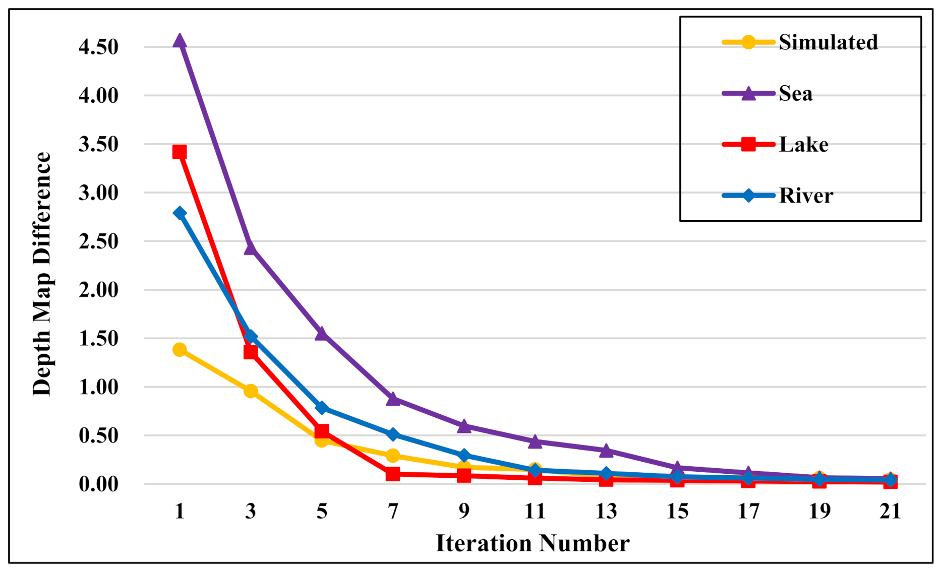
Furthermore, due to the specific iteration training scheme, the convergence of training process is also an important evaluation term for our proposed method. Obviously, depth map, referring to be the output of the depth estimation network, can be exploited as a reference to determine whether SUTDF has converged. Based on this viewpoint, we employed the discrepancy of depth maps between two iterations as a metric and a converging curve of the self-improving procedure has been plotted in Figure 15. From this figure we can know that the convergence speediness of framework is decreasing as the iteration number increases. Moreover, different datasets have disparate convergence iteration numbers which might be determined by the capacity of the dataset. In our research work, the framework trained with the lake water dataset requires the minimal convergence iteration number 7 while this dataset contains the least HSI pixels. On the contrary, the framework needs to go through 17 iterations for fitting the sea water dataset well, whose spatial solution is the highest among all the datasets.

Finally, we also calculate the execution time of different methods for an efficiency comparison and the associated results are presented in

Table 7. Average execution time (in seconds) of the compared methods for all the datasets.

Dataset	Execution Time (in seconds)
	CEM	MF	GBF	UTDF	UTD-Net
Simulated water	0.07272	0.02294	10.7841	15.8451	0.3518
Sea water	0.1276	0.3112	15.4782	24.1662	3.4795
River water	0.05086	0.1197	12.4119	19.4529	0.9172
Lake water	0.008924	0.004986	7.3684	11.4878	0.0818
Average	0.06502	0.1147	11.5017	17.7380	1.2076

The bold entries represent the best performance in each row.

. All the methods are carried out on the experimental environment mentioned in Section 4.2. It is worth mentioning that the learning-based methods always require considerable time in the training process. To make a more fair comparison, in this paper we denote the execution time as how much time a well-prepared method requires for deposing the given dataset. From Table 7 we find that the CEM method processes testing datasets with the least average execution time and land-based detection methods achieve the best efficiency performance for all the datasets. However, the detection performances of these methods are so poor that they can only detect the underwater targets being distinguishable from the water background. The reason accounting for this phenomenon is these land-based methods do not take care about the background interference. As for the proposed method, it can achieve the optimal detection performance with the lowest FAR, while its time duration is tolerable as well.

Considering every aspect of the detection results, we have confidence to conclude that SUTDF is capable of attaining an outstanding detection performance in most underwater scenarios.

4.5. Method Analysis

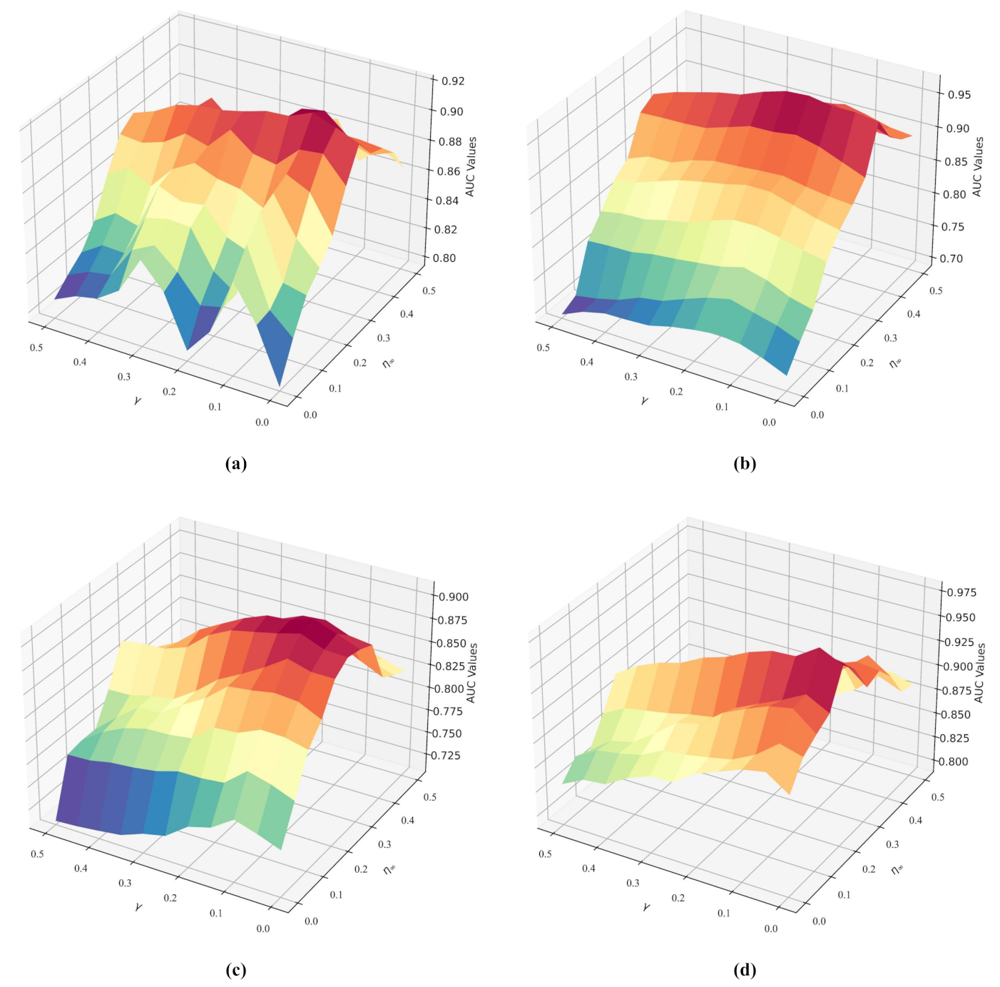
In this section, we finish certain specialized tests to evaluate the influences of human factors on the detection performance of our proposed method for a comprehensive method analysis. As mentioned above, the hyperparameters $\gamma$ and ${\eta }_{\infty }$ in Equation (11) may have great impact on the detection performance. To measure the influences of these two vital parameters, we perform the SUTDF on all the datasets with different combinations of parameter values. The 3D figures are exploited to depict the AUC values of $(P_D,P_F)$ of the different experimental result, which are demonstrated in Figure 16. The $\gamma$ and ${\eta }_{\infty }$ are both changed from 0 to 0.5 with a fixed step size of 0.05. Based on the visual inspection, it is easy to find that hyperparameter ${\eta }_{\infty }$ affects the detection results with a specific rule. This rule can be summarized as when the value of hyperparameters $\gamma$ is fixed, there always exists a local maximum in the AUC curve. In other words, if the hyperparameter $\gamma$ is not changed and the hyperparameter ${\eta }_{\infty }$ is smaller than the maximum point, increasing the value of ${\eta }_{\infty }$ will have a positive effect on the detection performance. On the contrary, when the hyperparameter ${\eta }_{\infty }$ is smaller than the maximum point, increasing the value of ${\eta }_{\infty }$ will undermine the final detection accuracy. Consequently, it is necessary to find the best value of hyperparameter ${\eta }_{\infty }$ before conducting experiments. Although intuitively, the analysis for this case can be interpreted as follows. The physical essence of hyperparameter ${\eta }_{\infty }$ is the confidence level which are utilized to verdict the properties of pixels (targets pixels or background pixels) according to depth estimation map. If the value of this parameter is set as a small value, only the pixels with high confidence will be selected, leading to a high FAR but a low detection rate. Reversely, a high detection rate but a low FAR will be achieved by SUTDF if we set this hyperparameter as a large value, where the corresponding pixels are picked out even if they do not have a rational confidence coefficient.

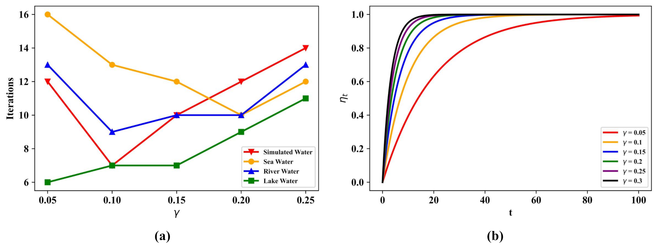
As for another hyperparameter $\gamma$, it might make no difference to the underwater detection results. However, as a parameter to control the grow rate of dynamic threshold ${\eta }_t$, $\gamma$ could make a contribution to alter the training process. In order to verify this hypothesis, we carry out some experiments with different $\gamma$ values and record the number of convergence iterations as the evaluation metric. The corresponding results are demonstrated in Figure 17, where Figure 17a depicts the relationship between $\gamma$ and the number of convergence iterations while Figure 17b shows the function curve of dynamic threshold ${\eta }_t$ with different $\gamma$. Obviously, from Figure 17a we can know that $\gamma$ can control the convergence speediness of SUTDF by the dynamic threshold ${\eta }_t$. As shown in Figure 17b, increasing the value of $\gamma$ makes the function curve of dynamic threshold ${\eta }_t$ process a larger gradient value in the early stage, resulting in drastic numerical changes for ${\eta }_t$. Meanwhile, ${\eta }_t$ is exploited as a sampling condition to construct the training dataset for the target detection network. Consequently, $\gamma$ eventually determines the growth speediness of the training dataset for the target detection network. In this way, if we enlarge the value of $\gamma$, the growth speediness of training dataset for target detection network will increase simultaneously, and then SUTDF is capable of reaching the terminal condition with less iterations. However, the value of $\gamma$ can be enlarged only in a limited range. When this value is set as too large, the training dataset will grow before the target detection network has been well-fitted, leading to an underfitting issue and finally decreasing the convergence speediness of SUTDF.

Based on above analyses, we can finally come to the conclusion that both ${\eta }_{\infty }$ and $\gamma$ are important parameters for SUTDF and these two parameters should be determined carefully before performing experiments. In terms of the parameter settings about these two parameters in our research work, relative information has been listed in Table 2 of Section 4.2.

5. Conclusions

In this paper, a novel underwater target detection framework named SUTDF was proposed. This specific framework was composed of three indispensable parts: Joint anomaly detector, depth estimation network, and target detection network. Due to the shortage of prior information about the underwater targets, a joint anomaly detector was developed with different typical anomaly methods to construct a target pixels subset from input HSI as the guidance dataset for depth estimation network. For the sake of achieving a low FAR and a high detection rate, the ensemble learning methodology was exploited to fuse the results of different anomaly detection methods. The experimental results demonstrated that the joint anomaly detector achieved the lowest FARs under different thresholds and could achieve a satisfying FAR even if the threshold was set as a small value.

After that, we designed a DNN in the autoencoder form to estimate the depth information for the given HSI in an unsupervised methodology based on the guidance dataset generated by the joint anomaly detector. In the encoder part of the depth estimation network, the 1-D CNN blocks were employed to address the spectral variety issue and to extract the locally invariant and discriminative spectral features. As for the decoder part, a bathymetric model was embedded into this structure, which contributed to the unsupervised training manner and made the SUTDF guarantee the same physical background as the existing research works. Then, a target detection network that could be implicitly explained as a binary classifier was established to detect underwater targets. The training datasets of this classifier were derived from the input HSI with the guidance of depth information map and an special under-sampling stage. Finally, considering the generalization capacities of the DNNs, we propose da self-improving iteration scheme to jointly perform the depth estimation and target detection for acquiring a more robust and accurate underwater detection result. Corresponding experiments validated that our proposed method possessed the capacity of achieving promising performance in most of the underwater scenarios.

References

1. Zhang, G.; Zhao, S.; Li, W.; Du, Q.; Ran, Q.; Tao, R. HTD-Net: A Deep Convolutional Neural Network for Target Detection in Hyperspectral Imagery. Remote Sens. 2020, 12, 1489. [Google Scholar] [CrossRef]
2. Hao, X.; Wu, Y.; Wang, P. Angle Distance-Based Hierarchical Background Separation Method for Hyperspectral Imagery Target Detection. Remote Sens. 2020, 12, 697. [Google Scholar] [CrossRef] [Green Version]
3. Ma, D.; Yuan, Y.; Wang, Q. Hyperspectral Anomaly Detection Based on Separability-Aware Sample Cascade. Remote Sens. 2019, 11, 2537. [Google Scholar] [CrossRef] [Green Version]
4. Shang, X.; Song, M.; Wang, Y.; Yu, C.; Yu, H.; Li, F.; Chang, C. Target-Constrained Interference-Minimized Band Selection for Hyperspectral Target Detection. IEEE Trans. Geosci. Remote Sens. 2020, 1–21. [Google Scholar] [CrossRef]
5. Gong, Z.; Zhong, P.; Yu, Y.; Hu, W. Diversity-Promoting Deep Structural Metric Learning for Remote Sensing Scene Classification. IEEE Trans. Geosci. Remote Sens. 2018, 56, 371–390. [Google Scholar] [CrossRef]
6. Gong, Z.; Zhong, P.; Yu, Y.; Hu, W.; Li, S. A CNN With Multiscale Convolution and Diversified Metric for Hyperspectral Image Classification. IEEE Trans. Geosci. Remote Sens. 2019, 57, 3599–3618. [Google Scholar] [CrossRef]
7. Zhong, P.; Gong, Z.; Shan, J. Multiple Instance Learning for Multiple Diverse Hyperspectral Target Characterizations. IEEE Trans. Neural. Netw. Learn Syst. 2020, 31, 246–258. [Google Scholar] [CrossRef]
8. Gong, Z.; Zhong, P.; Hu, W. Statistical Loss and Analysis for Deep Learning in Hyperspectral Image Classification. IEEE Trans. Neural. Netw. Learn Syst. 2021, 32, 322–333. [Google Scholar] [CrossRef] [Green Version]
9. Cheng, G.; Yang, C.; Yao, X.; Guo, L.; Han, J. When Deep Learning Meets Metric Learning: Remote Sensing Image Scene Classification via Learning Discriminative CNNs. IEEE Trans. Geosci. Remote Sens. 2018, 56, 2811–2821. [Google Scholar] [CrossRef]
10. Achard, V.; Foucher, P.-Y.; Dubucq, D. Hydrocarbon Pollution Detection and Mapping Based on the Combination of Various Hyperspectral Imaging Processing Tools. Remote Sens. 2021, 13, 1020. [Google Scholar] [CrossRef]
11. Zhan, T.; Song, B.; Xu, Y.; Wan, M.; Wang, X.; Yang, G.; Wu, Z. SSCNN-S: A Spectral-Spatial Convolution Neural Network with Siamese Architecture for Change Detection. Remote Sens. 2021, 13, 895. [Google Scholar] [CrossRef]
12. Zhao, C.; Li, C.; Feng, S.; Su, N.; Li, W. A Spectral–Spatial Anomaly Target Detection Method Based on Fractional Fourier Transform and Saliency Weighted Collaborative Representation for Hyperspectral Images. IEEE J. Sel. Top. Appl. Earth Obs. Remote Sens. 2020, 13, 5982–5997. [Google Scholar] [CrossRef]
13. Cheng, T.; Wang, B. Decomposition Model With Background Dictionary Learning for Hyperspectral Target Detection. IEEE J. Sel. Top. Appl. Earth Obs. Remote Sens. 2021, 14, 1872–1884. [Google Scholar] [CrossRef]
14. Bernabé, S.; Garcia, C.; Igual, F.D.; Botella, G.; Prieto-Matias, M.; Plaza, A. Portability Study of an OpenCL Algorithm for Automatic Target Detection in Hyperspectral Images. IEEE Trans. Geosci. Remote Sens. 2019, 57, 9499–9511. [Google Scholar] [CrossRef]
15. Gillis, D.B. Detection of underwater objects in hyperspectral imagery. In Proceedings of the 2016 8th Workshop on Hyperspectral Image and Signal Processing: Evolution in Remote Sensing (WHISPERS), Los Angeles, CA, USA, 21–24 August 2016; pp. 1–5. [Google Scholar]
16. Foucher, P.; Poutier, L.; Déliot, P.; Puckrin, E.; Chataing, S. Hazardous and Noxious Substance detection by hyperspectral imagery for marine pollution application. In Proceedings of the 2016 IEEE International Geoscience and Remote Sensing Symposium (IGARSS), Beijing, China, 10–15 July 2016; pp. 7694–7697. [Google Scholar]
17. Gillis, D.B. An Underwater Target Detection Framework for Hyperspectral Imagery. IEEE J. Sel. Top. Appl. Earth Obs. Remote Sens. 2020, 13, 1798–1810. [Google Scholar] [CrossRef]
18. Jay, S.; Guillaume, M.; Blanc-Talon, J. Underwater Target Detection with Hyperspectral Data: Solutions for Both Known and Unknown Water Quality. IEEE J. Sel. Top. Appl. Earth Obs. Remote Sens. 2012, 5, 1213–1221. [Google Scholar] [CrossRef]
19. Jay, S.; Guillaume, M. Underwater target detection with hyperspectral remote-sensing imagery. In Proceedings of the 2010 IEEE International Geoscience and Remote Sensing Symposium, Honolulu, HI, USA, 25–30 July 2010; pp. 2820–2823. [Google Scholar]
20. Fu, X.; Shang, X.; Sun, X.; Yu, H.; Song, M.; Chang, C.-I. Underwater Hyperspectral Target Detection with Band Selection. Remote Sens. 2020, 12, 1056. [Google Scholar] [CrossRef] [Green Version]
21. Brewin, R.J.W.; Devred, E.; Sathyendranath, S.; Lavender, S.J.; Hardman-Mountford, N.J. Model of phytoplankton absorption based on three size classes. Appl. Opt. 2011, 50, 4535–4549. [Google Scholar] [CrossRef]
22. Albert, A.; Mobley, C.D. An analytical model for subsurface irradiance and remote sensing reflectance in deep and shallow case-2 waters. Opt. Express 2003, 11, 2873–2890. [Google Scholar] [CrossRef]
23. Lee, Z.; Carder, K.L.; Mobley, C.D.; Steward, R.G.; Patch, J.S. Hyperspectral remote sensing for shallow waters. I. A semianalytical model. Appl. Opt. 1998, 37, 6329–6338. [Google Scholar] [CrossRef]
24. Lee, Z.; Carder, K.L.; Mobley, C.D.; Steward, R.G.; Patch, J.S. Hyperspectral remote sensing for shallow waters: 2. Deriving bottom depths and water properties by optimization. Appl. Opt. 1999, 38, 3831–3843. [Google Scholar] [CrossRef] [Green Version]
25. Gillis, D.B.; Bowles, J.H.; Montes, M.J.; Miller, W.D. Deriving bathymetry and water properties from hyperspectral imagery by spectral matching using a full radiative transfer model. Remote Sens. Lett. 2020, 11, 903–912. [Google Scholar] [CrossRef]
26. Werdell, P.J.; McKinna, L.I.W.; Boss, E.; Ackleson, S.G.; Craig, S.E.; Gregg, W.W.; Lee, Z.; Maritorena, S.; Roesler, C.S.; Rousseaux, C.S.; et al. An overview of approaches and challenges for retrieving marine inherent optical properties from ocean color remote sensing. Prog. Oceanogr. 2018, 160, 186–212. [Google Scholar] [CrossRef]
27. Qi, J.; Xue, W.; Gong, Z.; Zhang, S.; Yao, A. Hybrid Sequence Networks for Unsupervised Water Properties Estimation from Hyperspectral Imagery. IEEE J. Sel. Top. Appl. Earth Obs. Remote Sens. 2021, 14, 3830–3845. [Google Scholar] [CrossRef]
28. Reed, I.S.; Yu, X. Adaptive multiple-band CFAR detection of an optical pattern with unknown spectral distribution. IEEE Trans. Acoust. Speech Signal Process. 1990, 38, 1760–1770. [Google Scholar] [CrossRef]
29. Borghys, D.; Kåsen, I.; Achard, V.; Perneel, C. Comparative evaluation of hyperspectral anomaly detectors in different types of background. In Proceedings of the Algorithms and Technologies for Multispectral, Hyperspectral, and Ultraspectral Imagery XVIII, Baltimore, MD, USA, 24 May 2012; International Society for Optics and Photonics: Bellingham, WA, USA, 2012; p. 83902J. [Google Scholar]
30. Li, W.; Du, Q. Collaborative Representation for Hyperspectral Anomaly Detection. IEEE Trans. Geosci. Remote Sens. 2015, 53, 1463–1474. [Google Scholar] [CrossRef]
31. Carlotto, M.J. A cluster-based approach for detecting man-made objects and changes in imagery. IEEE Trans. Geosci. Remote Sens. 2005, 43, 374–387. [Google Scholar] [CrossRef]
32. Krizhevsky, A.; Sutskever, I.; Hinton, G.E. ImageNet classification with deep convolutional neural networks. In Proceedings of the 25th International Conference on Neural Information Processing Systems (NIPS), Lake Tahoe, NV, USA, 3–8 December 2012; pp. 1097–1105. [Google Scholar]
33. Wang, G.; Xie, X.; Lai, J.; Zhuo, J. Deep Growing Learning. In Proceedings of the 2017 IEEE International Conference on Computer Vision (ICCV), Venice, Italy, 22–29 October 2017; pp. 2831–2839. [Google Scholar]
34. Clark, R.; Swayze, G.; Wise, R.; Livo, E.; Hoefen, T.; Kokaly, R.; Sutley, S. USGS Digital Spectral Library splib06a: Us Geological Survey, Digital Data Series 231. Available online: http://speclab.cr.usgs.gov/spectral-lib.html (accessed on 22 March 2021).
35. Su, H.; Wu, Z.; Du, Q.; Du, P. Hyperspectral Anomaly Detection Using Collaborative Representation With Outlier Removal. IEEE J. Sel. Top. Appl. Earth Obs. Remote Sens. 2018, 11, 5029–5038. [Google Scholar] [CrossRef]
36. Harsanyi, J.C. Detection and Classification of Subpixel Spectral Signatures in Hyperspectral Image Sequences. Ph.D. Dissertation, University of Maryland, College Park, MD, USA, 1993. [Google Scholar]
37. Manolakis, D.G.; Shaw, G.A. Directionally constrained or constrained energy minimization adaptive matched filter: Theory and practice. In Proceedings of the Imaging Spectrometry VII, San Diego, CA, USA, 29 July–3 August 2002; pp. 57–64. [Google Scholar]
38. Richter, R.; Schläpfer, D. Geo-atmospheric processing of airborne imaging spectrometry data. Part 2: Atmospheric/topographic correction. Remote Sens. Lett. 2002, 23, 2631–2649. [Google Scholar] [CrossRef]
Figure 1. An illustration of the generation process for sensor-observed spectrum.
Remotesensing 13 01721 g001
Figure 2. The general framework of our proposed method.
Remotesensing 13 01721 g002
Figure 3. The overview of the autoencoder-form depth estimation network.
Remotesensing 13 01721 g003
Figure 4. The spectral distances between sensor-observed spectrum r ( λ ) and land-based spectrum r B ( λ ) with different depth information.
Remotesensing 13 01721 g004
Figure 5. The constituents of the target detection network.
Remotesensing 13 01721 g005
Figure 6. Synthetic data based on simulated turbid water for experiment. (a) Image scene of simulated turbid water; (b) distribution of desired targets; and (c) spectra of desired targets and main backgrounds.
Remotesensing 13 01721 g006
Figure 7. Synthetic data based on sea water for experiment. (a) Image scene of sea water; (b) distribution of desired targets; and (c) spectra of desired targets and main backgrounds.
Remotesensing 13 01721 g007
Figure 8. Synthetic data based on lake water for experiment. (a) Image scene of lake water; (b) distribution of desired targets; and (c) spectra of desired targets and main backgrounds.
Remotesensing 13 01721 g008
Figure 9. Synthetic data based on river water for experiment. (a) Image scene of river water; (b) distribution of desired targets; and (c) spectra of desired targets and main backgrounds.
Remotesensing 13 01721 g009
Figure 10. The FPR of different anomaly detection methods with some certain thresholds.
Remotesensing 13 01721 g010
Figure 11. The underwater target detection results of compared methods for the all datasets. (a) Ground truth of simulated, sea, river, and lake water datasets. (b) SUTDF. (c) UTDF. (d) GBF. (e) CEM. (f) MF.
Remotesensing 13 01721 g011
Figure 12. The ROC curves of ( P D , P F ) for the compared underwater target detection methods on a (a) simulated water dataset, (b) sea water dataset, (c) river water dataset, and (d) lake water dataset.
Remotesensing 13 01721 g012
Figure 13. The ROC curves of ( P F , T h r e s h o l d ) for the compared underwater target detection methods on a (a) simulated water dataset, (b) sea water dataset, (c) river water dataset, and (d) lake water dataset.
Remotesensing 13 01721 g013
Figure 14. The results of exploring the generalization ability of each depth estimation network.
Remotesensing 13 01721 g014
Figure 15. The converging curve of the self-improving procedure for all the datasets.
Remotesensing 13 01721 g015
Figure 16. The 3D plots for AUC values of ( P D , P F ) of the different experiments on a (a) simulated water dataset, (b) sea water dataset, (c) river water dataset, and (d) lake water dataset.
Remotesensing 13 01721 g016
Figure 17. The results of hyperparameter γ analysis experiments. (a) The relationship between γ and the number of convergence iterations; (b) The function curve of dynamic threshold η t with different γ .
Remotesensing 13 01721 g017