Article

Fusing Precipitable Water Vapor Data in CHINA at Different Timescales Using an Artificial Neural Network

1
School of Geodesy and Geomatics, Wuhan University, Wuhan 430079, China
2
Chinese Academy of Meteorological Sciences, Beijing 100081, China
*
Author to whom correspondence should be addressed.
Remote Sens. 2021, 13(9), 1720; https://doi.org/10.3390/rs13091720
Submission received: 23 March 2021 / Revised: 23 April 2021 / Accepted: 28 April 2021 / Published: 29 April 2021

Abstract

:
Global climate change has noticeable influences on the water vapor redistribution in China, which is embodied by the fact that both wetting and drying tendencies were observed across China. This poses the necessity to monitor and understand the water vapor evolution in China. However, observations of water vapor from different techniques are subjected to systematic biases, different spatiotemporal resolutions and coverages, and different accuracy, which would hamper their joint use, potentially leading to contradictory conclusions when using different techniques. Data fusion is a promising way to address this problem. Some scholars have proposed several methods to fuse multi-source PWV data in China region, such as the enhanced spatial and temporal adaptive reflectance fusion model, the hybrid PWV fusion model, and the linear calibration model. Although these models can produce PWV products with improved accuracy, they still have some shortcomings, such as no consideration for spatial or temporal variations in bias or inevitably impose some biases inaccurate information since assumptions made for interpolations are imperfect. In this study, we use the high-quality Global Navigation Satellite System (GNSS) precipitable water vapor (PWV) to calibrate and optimize the Moderate-resolution Imaging Spectroradiometer (MODIS) and the European Centre for Medium-Range Weather Forecasts ReAnalyses 5 (ERA5) PWV in 2018–2019 through a Generalized Regression Neural Network (GRNN) at annual, quarterly, and monthly timescales. Validation results demonstrate that modifying the MODIS and ERA5 PWV at the monthly timescale results in the best accuracy. In the monthly experiment, the average bias, standard deviation (STD), and root mean square (RMS) error of modified MODIS PWV are 0.0 mm, 2.6 mm, and 2.6 mm, respectively. The percentage improvement is as high as 50% in terms of RMS compared to the original MODIS PWV. It becomes 0.0 mm, 1.7 mm, and 1.7 mm for the modified ERA5 PWV and the percentage improvement is 40%. Since the biases among different products are well-calibrated and the accuracy of MODIS and ERA5 PWV is improved to the same level of GNSS PWV, we can fuse them by simply merging them. Finally, we generate a new product of PWV in China with a temporal resolution of 1 day, a spatial resolution better than 31 km, and an accuracy better than 2.7 mm, which will serve as a high-quality product for investigating the water vapor redistribution under a changing climate.

Graphical Abstract

1. Introduction

Water vapor plays an important role in climate change and water cycling at various scales. In the past decades, global climate change has exerted noticeable influences on the water vapor distribution in China, which is evidenced by the fact that some regions in western and southern China are becoming wetter while some regions in eastern China are becoming drier [1,2]. Besides being an indicator of climate change, water vapor also affects the propagation of radio signals by causing path bending and time delay, which is known as wet tropospheric delay in radio-based geodetic techniques including Global Navigation Satellite System (GNSS) and Interferometric Synthetic Aperture Radar (InSAR). Namely, water vapor is an error source in radio-based geodetic techniques, and its effect should be corrected. Therefore, monitoring the water vapor is a basic requirement for understanding the change in climate and water cycling, and improving the accuracy of radio-based geodetic techniques.
Precipitable water vapor (PWV) is commonly used to describe the amount of water vapor in the atmosphere and is defined as the vertically integrated water vapor over unit area expressed by equivalent water height. PWV can be retrieved from observations and models. The observation methods include radiosonde, satellite remote sensing [3,4,5], GNSS [6,7,8], and water vapor radiometer, etc. The model methods mainly refer to the numerical weather prediction models, including European Centre for Medium-Range Weather Forecasts (ECMWF) [9,10], National Centers for Environmental Prediction [9,11], etc. Moderate-resolution Imaging Spectroradiometer (MODIS) PWV is one kind of satellite remote sensing PWV, which has a high spatial resolution (1–5 km) but its quality is affected by weather and ground surface conditions. Scientists have found that the accuracy of MODIS PWV is 5–6 mm in the China area [12,13], which is much worse than in the US area (2–4 mm) [14,15]. The accuracy of GNSS PWV is typically 1–2 mm [6,7,16,17], but its spatial resolution is limited by the sparse station deployment. The model-simulated PWV has a medium spatiotemporal resolution but its accuracy is dependent on the density and quality of the assimilated observations. Because of the systematic biases among different methods, different spatial and temporal resolutions and coverages, care has to be taken for the joint use of different PWV data sources. Otherwise, contradictory conclusions may be obtained when using different individual PWV data sources [15,18].
Data fusion is a promising way to address this problem. Li et al. [14] used a Global Position System-derived correction linear fit model to modify the accuracy of MODIS PWV and produce a regional 1 km × 1 km water vapor field in Southern California. Lindenbergh et al. [19] fused Medium Resolution Imaging Spectrometer PWV and GNSS PWV based on ordinary kriging interpolation in western Europe and the results were beneficial to numerical weather prediction. Alshawaf et al. [20] built PWV maps by fusing Persistent Scatterer InSAR and GNSS data over the region of Upper Rhine Graben in Germany and France and used the kriging geostatistical interpolation technique to produce continuous grids of PWV. Alshawaf et al. [21] used a fixed-rank kriging method to fuse GNSS PWV, InSAR PWV, and the Weather Research and Forecasting model simulated PWV in Europe and found that PWV maps inferred by the data fusion have a better quality than those inferred from a single data source. Zhang et al. [15] proposed a method based on spherical cap harmonic model and Helmert variance component estimation to fuse GNSS, MODIS, and ECMWF ReAnalyses 5 (ERA5) PWV, and obtained high accuracy (2 mm) in North America. Li and Long [22] combined MODIS and ERA5 PWV to generate PWV products in the upper reaches of the Brahmaputra river from 2007 to 2013, and the generated PWV products had good consistency with the Global Position System measurements. Zhao et al. [18] proposed a PWV fusion model in China based on the polynomial fitting and spherical harmonic function, and the results showed that the mean root square (RMS) of the hybrid PWV fusion model was less than 3 mm in any areas of China in all four seasons. Bai et al. [23] proposed a linear calibration model which uses GNSS PWV to calibrate MODIS PWV in mainland China, and the results showed obvious improvements in calibrated MODIS PWV. Some of the above methods are based on interpolation approach, which may inevitably impose biases or inaccurate information due to the imperfect assumptions made for the interpolation [24]. Some of the above methods only calibrate a global bias and do not consider spatial or temporal variations in bias. Moreover, the MODIS PWV has poor quality in China [12,13], which makes it unqualified for the investigation of subtle PWV variation in China. Because of these problems, efforts are needed to produce high-quality PWV in China. The method proposed by Zhang et al. [24] does not need any prior information or assumption which could avoid introducing biases before fusing and can fully consider the spatial variation of the systematic biases between different PWV data.
In this study, we use the Generalized Regression Neural Network (GRNN) method proposed by Zhang et al. [24] to fuse the PWV data from GNSS, MODIS, and ERA5 to generate a unified high-quality PWV dataset in the land area of China. Different from Zhang et al. [24] that fused PWV data in North America at an annual scale, this study fuses the PWV data at annual, quarterly, and monthly scales in China in an attempt to find out the best timescale for PWV fusion in China. Through this study, we aim to generate a unified PWV product for China with improved accuracy and spatial resolutions and thus providing a better PWV product. The new PWV product not only can be useful for the application of earth observation such as performing the tropospheric refraction correction of InSAR observation, but it will also allow more detailed monitoring of water vapor over China. Besides, this PWV product can also be a data source of numerical weather forecasting and help researchers better study the circulation of water vapor over China.

2. Research Area and PWV Data
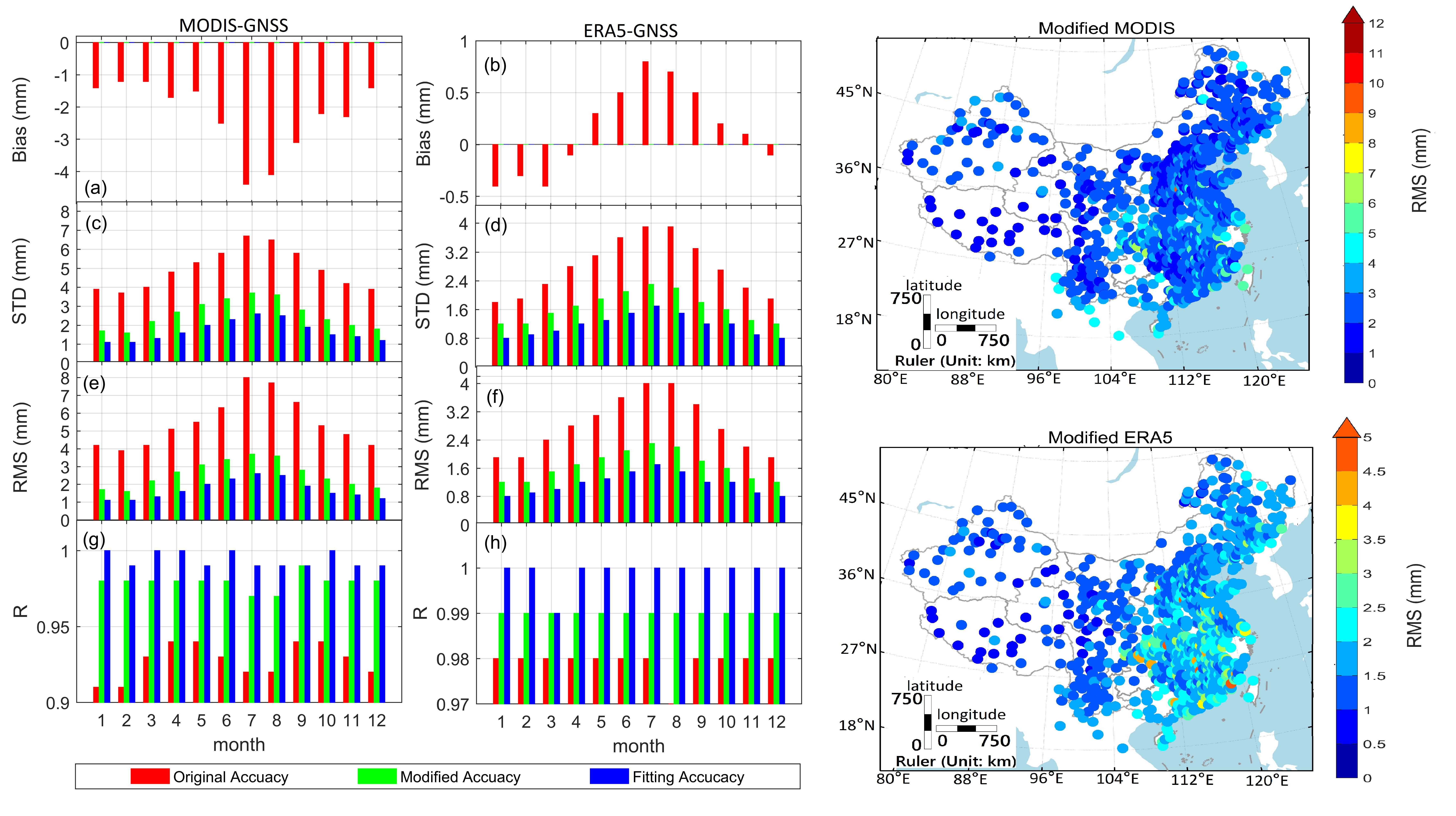
2.1. Research Area

Our research area is in the land area of China which is shown in Figure 1 with GNSS stations and radiosonde stations. The topography of the research area is high (>4000 m) in the west and decreases sharply to the east. The climate in the research area is complex and diverse because of the tremendous differences in latitude, longitude, and altitude. These conditions lead to complex variations in PWV in the research area. The GNSS PWVs used in this study are collected by 11 stations from the International GNSS Service (IGS) network, 1084 stations from China Meteorological Administration (CMA) GNSS network, and 257 Crustal Movement Observation Network of China (CMONOC) GNSS stations. Six GNSS stations coexist in both the CMONOC and IGS network. There are 89 radiosonde stations used to assess the accuracy of ERA5 temperature, ERA5 pressure, and GNSS PWV. The radiosonde data are derived from the Integrated Global Radiosonde Archive Version 2 dataset and includes pressure, temperature, relative humidity, and other parameters with a temporal resolution of twice or four times daily (ftp://ftp.ncdc.noaa.gov/pub/data/igra/ (accessed on 25 April 2020)).

2.2. Multi-Source PWV

2.2.1. GNSS PWV

As shown in Figure 1a, the GNSS PWVs have three sources, namely, IGS, CMA, and CMONOC. The CMA GNSS PWV is provided directly by the Meteorological Observation Center of CMA which has a time resolution of 1 h. The strategy used to process CMA GNSS data can be found in Liang et al. [25]. The CMONOC and IGS GNSS observations are processed by a Precise Point Positioning (PPP) software developed by Yao Yibing’s group at Wuhan University and the principle can be seen in Yao et al. [26]. The IGS Real-Time Service IGS03 track and clock products are used for data processing. Kouba and Heroux [27] method is used to correct antenna phase center migration and variation, phase windings, earth tides, earth rotation, ocean tides, and relativistic effects. The product of Center for Orbit Determination in Europe [28] corrects discrepancies in the differential code. The ionospheric delay is corrected to the first order by using the ionospheric two-frequency phase observation combination. The higher-order error of the ionosphere is ignored. Then, we obtain the GNSS Zenith Total Delay (ZTD) with a time resolution of 30 min. We compare it with the IGS-released GNSS ZTD, and the bias, the standard deviation (STD) and the RMS are −1.0 mm, 8.9 mm, and 9.0 mm, respectively.
The GNSS ZTD includes zenith hydrostatic delay (ZHD) and zenith wet delay (ZWD). The ZHD could be obtained by the Saastamoinen model [29] which needs surface pressure. The transformational relation between ZWD and PWV can be found in Xiong et al. [11] which needs temperature. The needed temperature and pressure are interpolated from ERA5 data and its accuracy is assessed by the Radiosonde data. The linear interpolation in the vertical direction and bilinear interpolation in the horizontal direction are applied to interpolate ERA5 data for a Radiosonde (GNSS) station location to obtain the temperature and pressure. The accuracy of temperature in terms of bias, STD, and RMS are 0.26 K, 2.25 K, and 2.27 K, respectively. It becomes 0.57 hPa, 1.68 hPa, and 1.77 hPa for pressure.
Finally, we obtain the IGS and CMONOC GNSS PWV. We call the PWV processed by PPP software as PPP PWV and PWV from CMA as CMA PWV. The Radiosonde data are also used to assess PPP PWV and CMA PWV. The method to obtain Radiosonde PWV at GNSS station location can be found in Appendix A. The accuracy of PPP PWV in terms of bias, STD, and RMS is 0.9 mm, 1.7 mm, and 1.9 mm, respectively. It becomes −0.3 mm, 1.6 mm, and 1.6 mm for CMA PWV. Both CMA PWV and PPP PWV have an accuracy within 2 mm, which indicates that the GNSS PWV can be used as the reference in the future to calibrate the MODIS PWV and ERA5 PWV for fusion.

2.2.2. ERA5 PWV

The ERA5 data are the latest generation of global climate reanalysis data released by ECMWF [30]. Compared with the previous generation ERA-Interim, the temporal resolution is improved from 6 to 1 h and the spatial resolution improved from 0.75° to 0.25°. The height information of the ERA5 grids is obtained from the Shuttle Radar Topography Mission Digital Elevation Model (STRM DEM) Version 4.1 data with a spatial resolution of 250 m [31,32]. The height system in STRM DEM is orthometric height. Therefore, the height information for the ERA5 PWV is based on the orthometric height.

2.2.3. MODIS PWV

MOD05_L2 provides two types of MODIS PWV products: Near Infrared PWV with a spatial resolution of 1 km and Infrared PWV with a resolution of 5 km. We only use the Near Infrared PWV, since the accuracy of Near Infrared PWV is better than Infrared PWV [33,34]. Considering the spatial resolution of ERA5 PWV and GNSS PWV, we downscale the spatial resolution of Near Infrared PWV from 1 km to 5 km, which can effectively reduce the computational burden. In addition, the data quality of the MODIS PWV products is greatly affected by the weather and surface conditions. So only the Near Infrared PWV on land under cloudless conditions is used. To avoid the effect of anomalous data, we exclude the data in the top 0.5% and negative values. We also use the SRTM DEM to provide height information for the MODIS PWV.
In this study, the GNSS, MODIS, and ERA5 PWV are fused to generate a unified PWV product. Since the GNSS PWV is based on the ellipsoidal height while the MODIS and ERA5 PWV are based on the orthometric height, we need to unify the height system. We use the method in Li et al. [35] to make height corrections to the GNSS PWV so that all the PWV data are based on the orthometric height.

3. GRNN Method for PWV Fusion

We use the GRNN method to fuse GNSS, MODIS, and ERA5 PWV. In addition to the annual fusion as in Zhang et al. [24], we also implement the fusions at the quarterly and monthly timescales to explore more subtle variations in the PWVs.

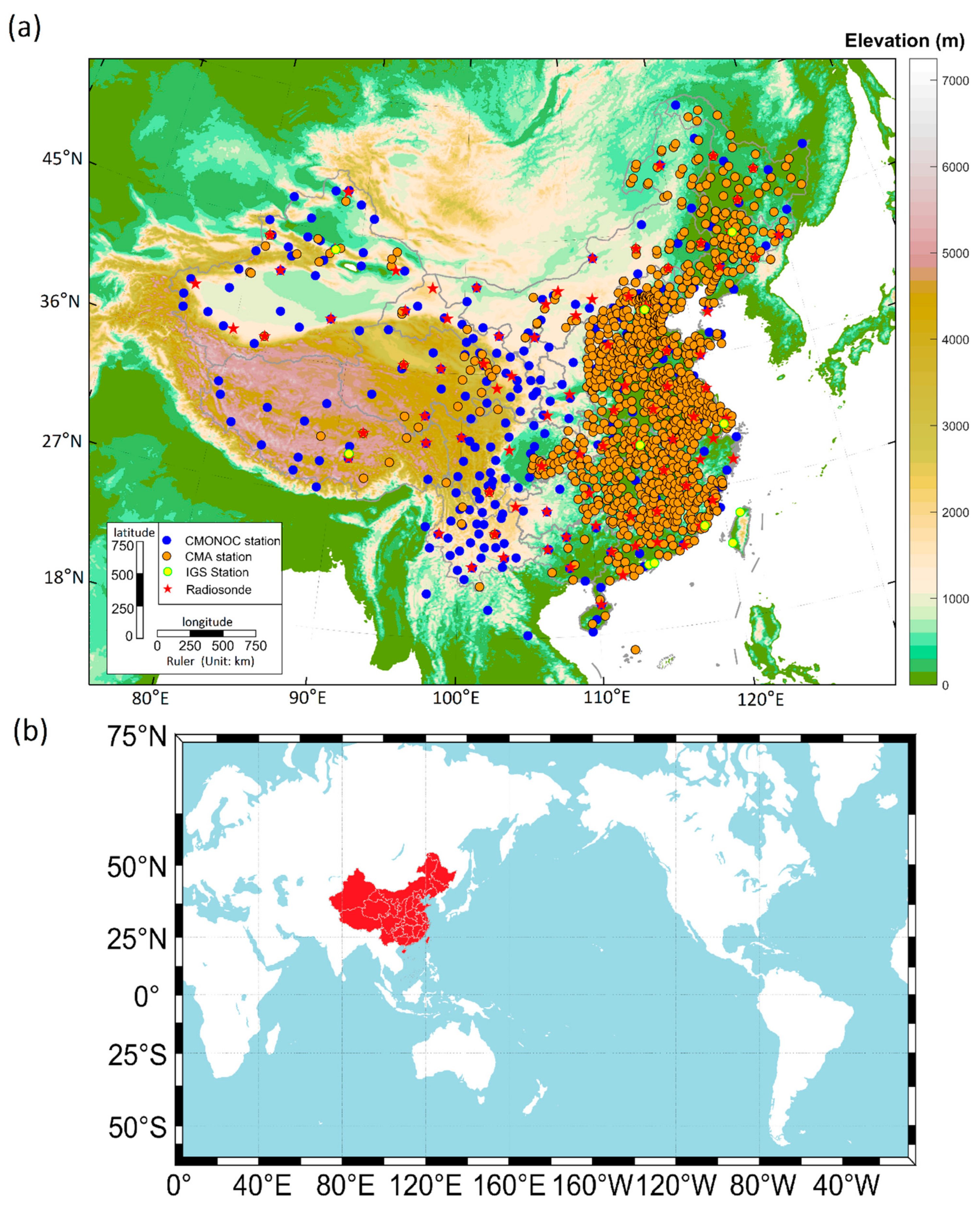
3.1. Generalized Regression Neural Network

The GRNN was proposed by Specht in 1991 [36] which is based on non-parametric regression and uses sample data as a posterior condition. GRNN has a four-layer structure with an input layer, a pattern layer, a summation layer, and an output layer. The spread parameter in the pattern layer is the only hyperparameter in GRNN which needs to be set at first.
The advantage of the GRNN model is that no model parameters need to be trained, so the convergence speed is fast. In addition, the GRNN is based on radial basis function and has good nonlinear approximation performance. The disadvantage of the GRNN is its high computational complexity and space complexity.

3.2. Model Structure

Figure 2 shows the model structure of the GRNN model for PWV fusion. The input layer has five neurons corresponding to the longitude, latitude, height, time, and MODIS (ERA5) PWV. There is only one neuron in the output layer which is the GNSS PWV or the modified MODIS (ERA5) PWV. The number of neurons in the pattern layer is equal to the number of observations. Considering that ERA5 PWV, MODIS PWV, and GNSS PWV have systematic differences and different error characteristics, we take GNSS PWV as the reference values and use them to improve the MODIS and ERA5 PWV, respectively.

3.3. PWV Data Matching

To form input-output samples, we need to interpolate the dense MODIS (ERA5) PWV to the location of GNSS PWV. For temporal interpolation, we interpolate the GNSS PWV and ERA5 PWV to the epoch of MODIS PWV using a simple linear interpolation. For the spatial interpolation, we use a spherical cap harmonic model to fit the MODIS (ERA5) PWV, which is then used to compute PWV at the GNSS stations. For the ERA5 PWV, the pole of the spherical cap is (35.5327° N, 104.1477° E), and the half angle of the spherical cap is 35°. Because the area covered by MODIS PWV data at different epochs is inconsistent, the pole of the spherical cap is set at the center of the available MODIS PWV. The order of the spherical cap harmonic model is set to 5 for the MODIS PWV while it is 10 for the ERA5 PWV. These settings guarantee that the corresponding spherical cap harmonic model has the smallest misfit RMS error. After temporal and spatial interpolations, the MODIS (ERA5)-GNSS PWV pairs are obtained. Finally, we obtain 353,271 MODIS-GNSS pairs and 960,047 ERA5-GNSS pairs in 2018 and 2019. The monthly number of MODIS-GNSS pairs fluctuates between 9025 and 23,667, while that of ERA5-GNSS pairs fluctuates between 28,474 and 61,961.
Since the data quality of the samples affects the model performance, simple quality control is performed. We first calculate the bias and STD of the differences between the interpolated MODIS (ERA5) PWVs and GNSS PWVs and then use bias ±3 STD as the threshold to reject any pair whose corresponding difference is larger than the threshold. Finally, 7345 MODIS-GNSS PWV pairs and 10,238 ERA5-GNSS PWV pairs are removed, and the remaining samples are used to train the model. The remaining MODIS-GNSS pairs fluctuate between 8785 and 23,387 in one month while the ERA5-GNSS pairs fluctuate between 28,449 and 61,599. The average bias, STD, RMS, and correlation coefficient (R) between the MODIS (ERA5) PWV in 2018 and 2019 after excluding outliers are given in Table 1. It is seen that MODIS PWV tends to be larger than GNSS PWV while ERA5 PWV is smaller than GNSS PWV in terms of bias. The accuracy of MODIS PWV in China region is poorer than that of ERA5 PWV in terms of RMS.

3.4. Constructing the GRNN Models

After obtaining the MODIS-GNSS PWV pairs and ERA5-GNSS PWV pairs in the research area in 2018 and 2019, we use the GRNN method to fuse them at annual, quarterly, and monthly scales. Because the spread parameter in the pattern layer has a great influence on the model results, we use an enumeration algorithm to determine the optimal spread parameter, and the results can be found in Appendix B. In Appendix B, we set a series of optional spread parameters to test the GRNN model and present the model performance against spread parameter values.
In machine learning, cross-validation is often used to test the accuracy of algorithms. K-fold cross-validation has been widely used in machine learning [37,38,39]. Using K-fold cross-validation, every sample can be used for training or testing. In this study, the 10-fold cross-validation is used to test the model. The ten-fold cross-validation randomly divides the dataset into ten equal parts, and selects one of them as the test data and the other nine as the training data without duplication. After repeating ten times, the average statistical results can be used to evaluate the accuracy of the model.

4. Results

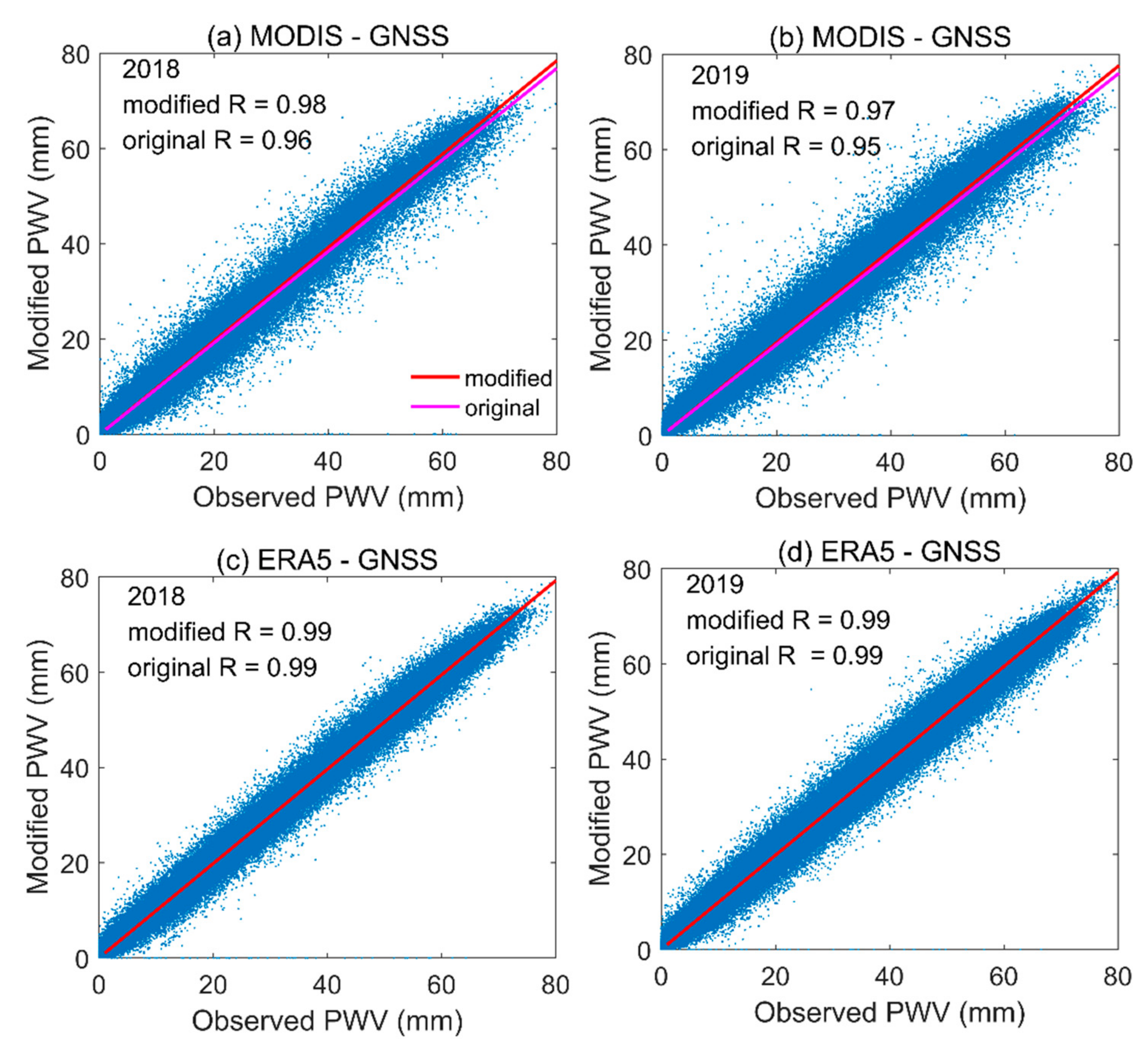
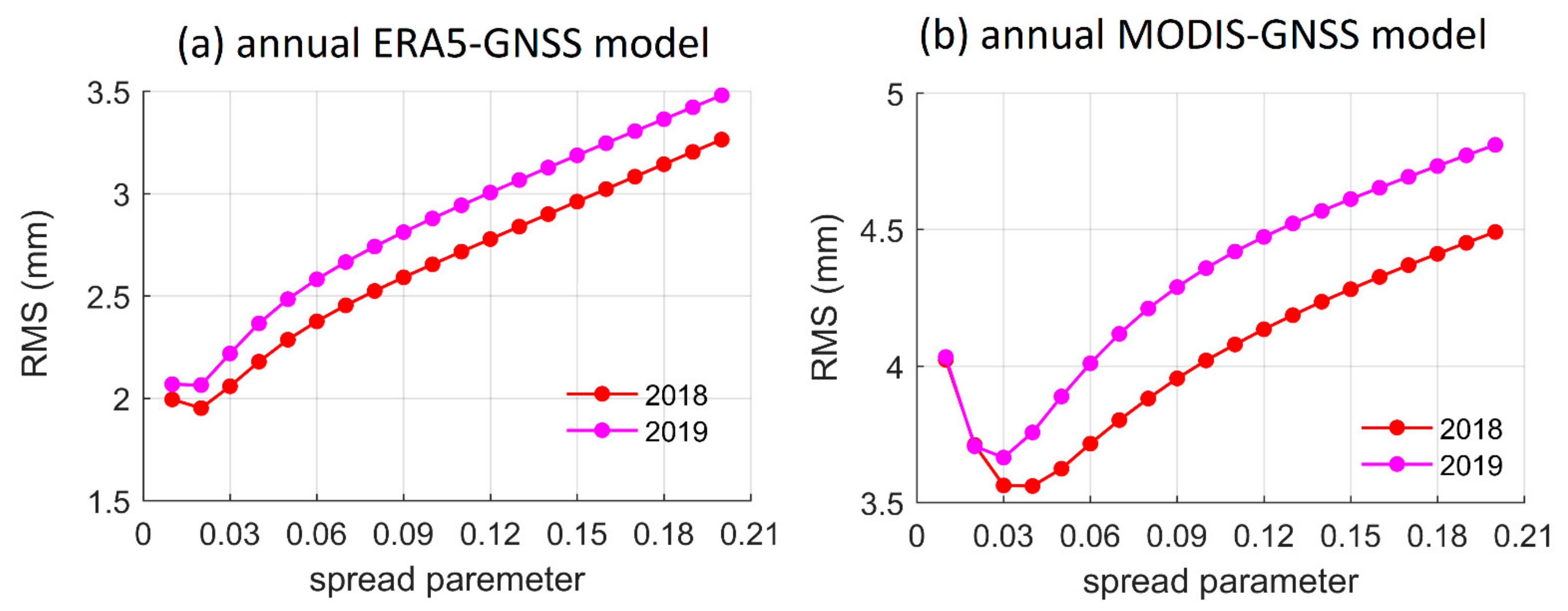
4.1. Model Performance at Annual Timescale

We use the samples in 2018 and 2019, respectively, to train and test the MODIS-GNSS PWV model and the ERA5-GNSS PWV model. We train the models using data in a whole year, and obtain a GRNN model in 2018 and another one in 2019.
Table 2 presents the average testing results when training the model based on annual data in 2018 and 2019 with the optimal spread parameter given in Appendix B. Compared to the RMS values of the original datasets given in Table 1, the accuracy in terms of RMS is improved by 1.9 mm for MODIS PWV and 1.0 mm for ERA5 PWV. The bias between the modified MODIS (ERA5) PWV and the GNSS PWV is close to 0, indicating that the systemic difference between them has been eliminated after training. The scatter plots of the modified MODIS (ERA5) PWV versus GNSS PWV in the annual models are shown in Figure 3. Both the modified MODIS and ERA5 PWV have a better correlation with the GNSS PWV.

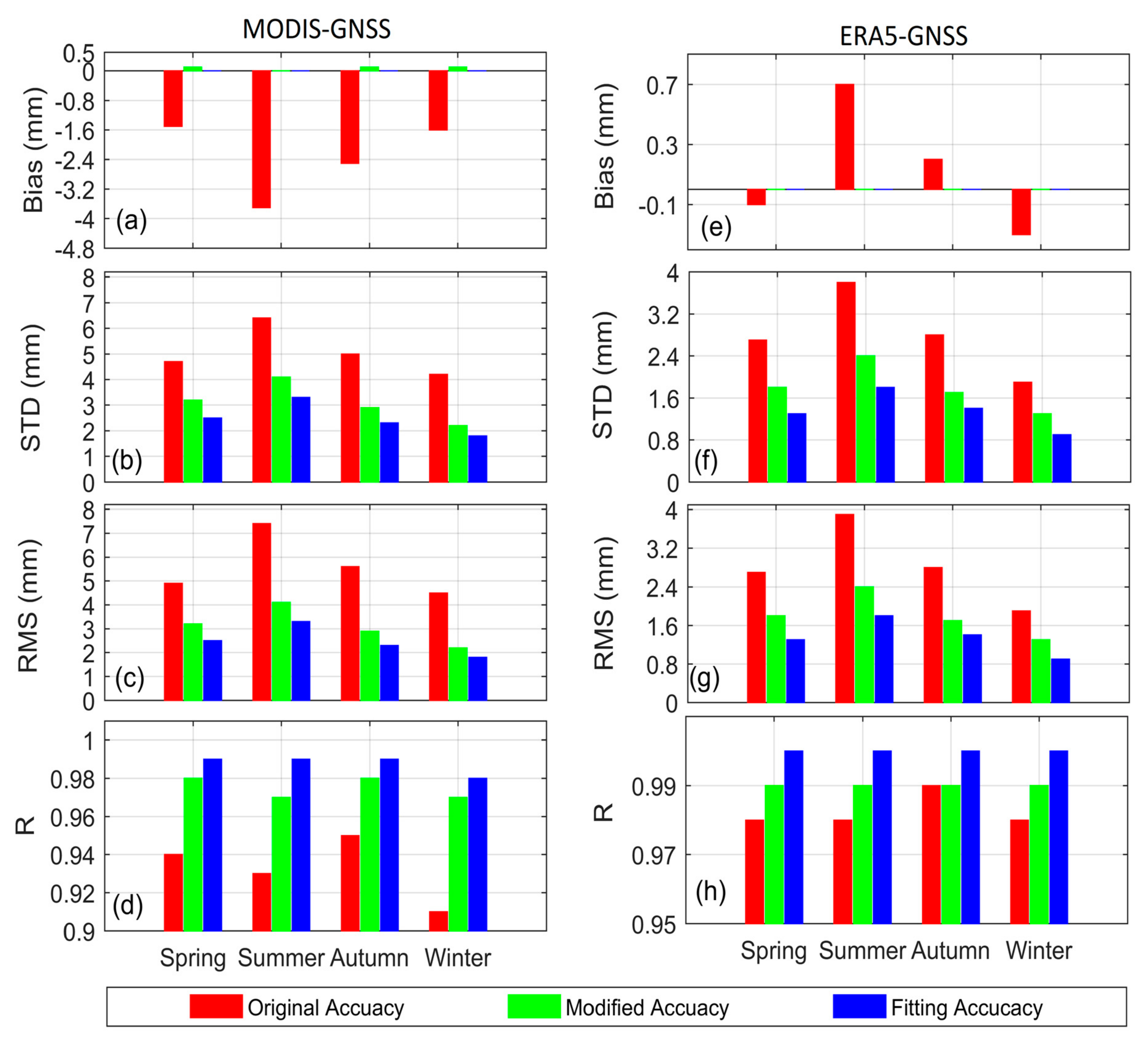
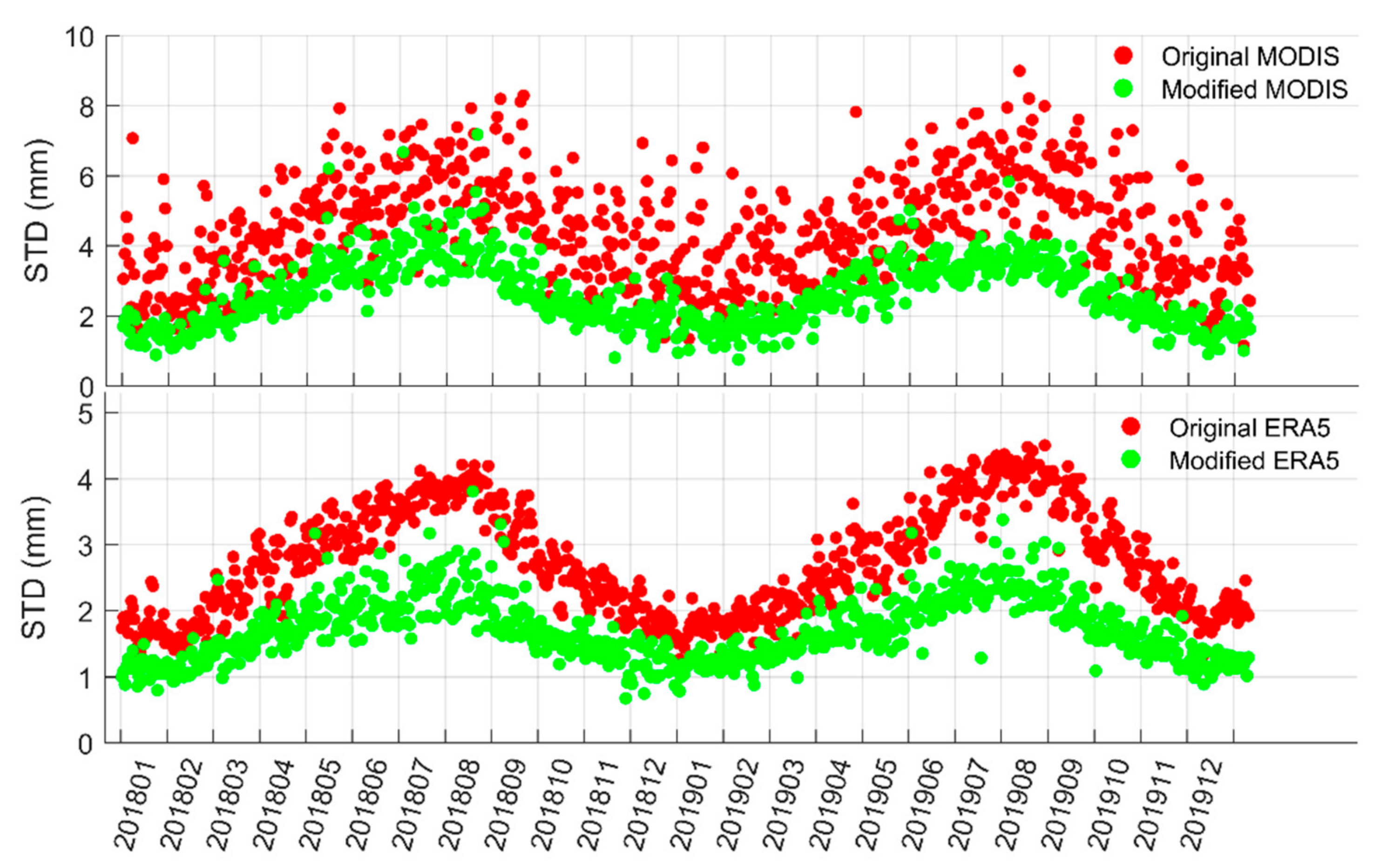
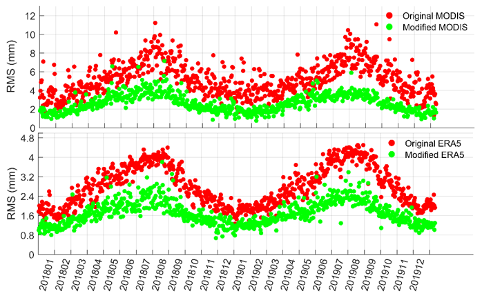
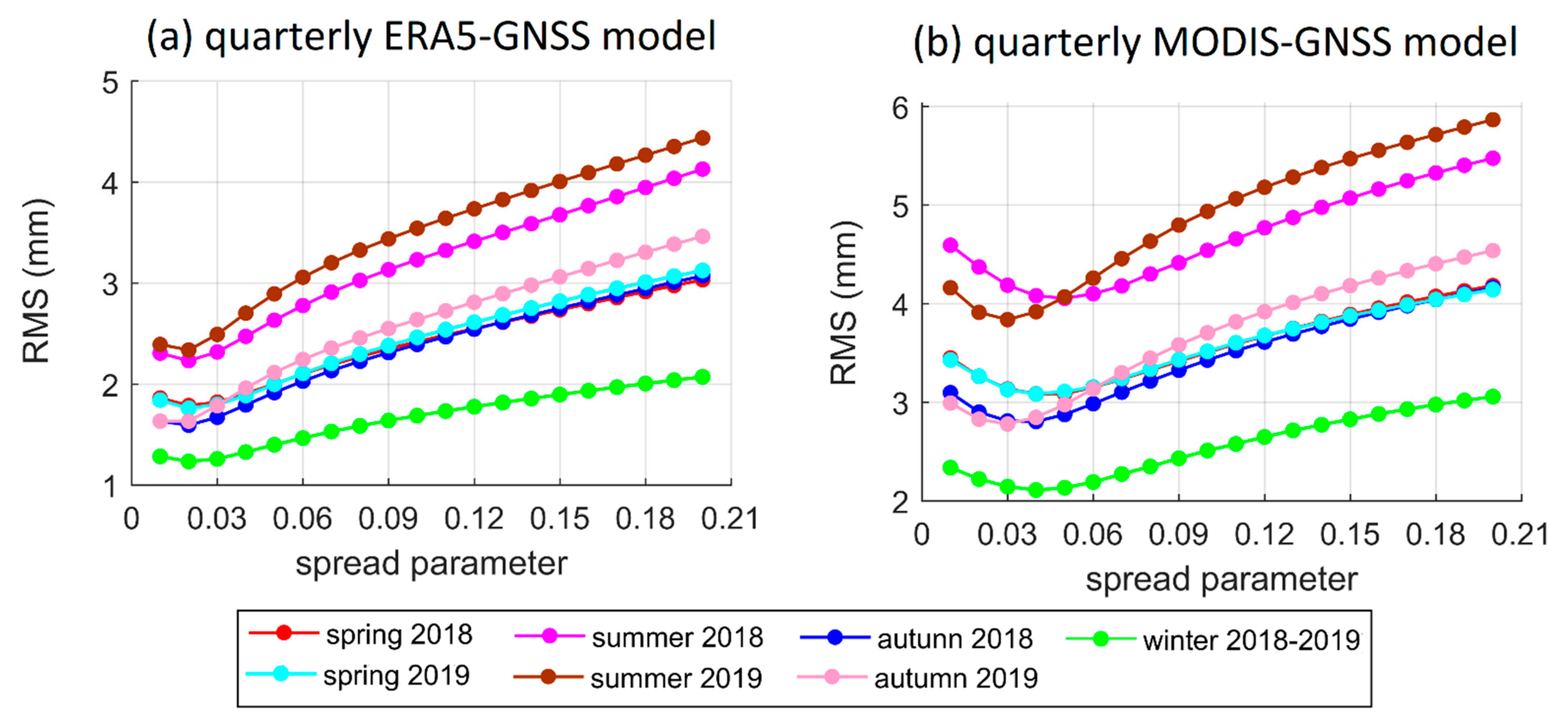
4.2. Model Performance at Quarterly Timescale

We also train and test the GRNN models based on quarterly MODIS (ERA5)-GNSS PWV samples. This means we use the samples in every individual quarter to construct a corresponding quarterly GRNN model. In this manuscript, spring is defined from March to May, summer from June to August, autumn from September to November, and winter from December to February.
Table 3 presents the overall performance of the quarterly models with the optimal spread parameter given in Appendix B. The systematic difference between MODIS (ERA5) PWV and GNSS PWV is also eliminated after training since the bias is close to 0. The accuracy in terms of RMS of the quarterly model is improved by 2.5 mm for MODIS PWV and 1.1 mm for ERA5 PWV, which are better than the improvement achieved by the annual models.
Figure 4 shows the average bias, STD, RMS, and R of the quarterly models in different seasons. The original accuracy in terms of RMS for MODIS PWV in the spring and autumn is 5–6 mm, and it is even worse with RMS increasing to about 7.5 mm in the summer. The quarterly MODIS-GNSS PWV models effectively improve the accuracy of the modified MODIS PWV, as demonstrated in Figure 4c. The accuracy improvement in terms of RMS for MODIS PWV in four seasons is 1.8 mm (spring), 3.3 mm (summer), 3.0 mm (autumn), and 2.3 mm (winter), respectively. The accuracy improvement in terms of RMS in the spring is slightly less than that of the annual model (1.9 mm), but the RMS in the Spring quarterly model is 3.6 mm which is smaller than that of the annual model (3.8 mm). These results indicate that the seasonal differences are accounted for by the quarterly models. As shown in Figure 4d, the R has improved in all four seasons, especially in the winter.
For the ERA5-GNSS quarterly models, the accuracy improvement in terms of RMS in four seasons is 0.9 mm (spring), 1.5 mm (summer), 1.3 mm (autumn), and 0.7 mm (winter), respectively. The accuracy improvement in terms of RMS in the summer and autumn is better than that of the annual model (1.0 mm). Although the accuracy improvement in terms of RMS in spring and winter is less than the annual model, the RMSs of the quarterly models in spring and winter are 1.8 mm and 1.3 mm, respectively, which are smaller than that of the corresponding annual model (2.0 mm). Those results indicate that considering the seasonal differences can improve the model performance, which is conducive to the generation of high-quality PWV products in China. The systematic difference between the modified ERA5 PWV and GNSS PWV is close to 0, which indicates that the ERA5-GNSS quarterly model can also eliminate the systematic difference. In addition, as shown in Figure 4h the correlation coefficient R between the modified ERA5 PWV and the GNSS PWV increases to 0.99 by the quarterly models.

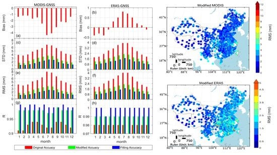
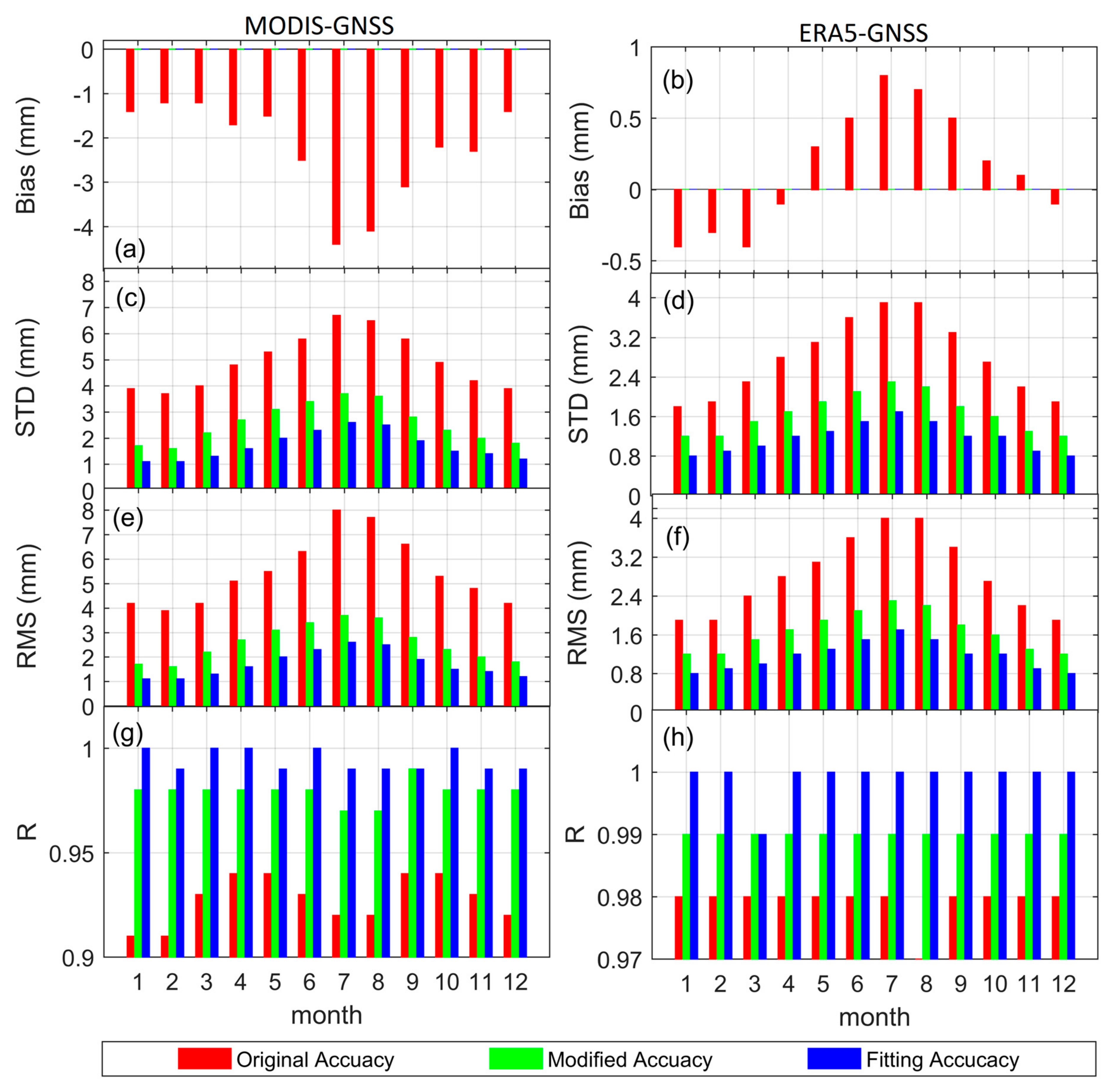
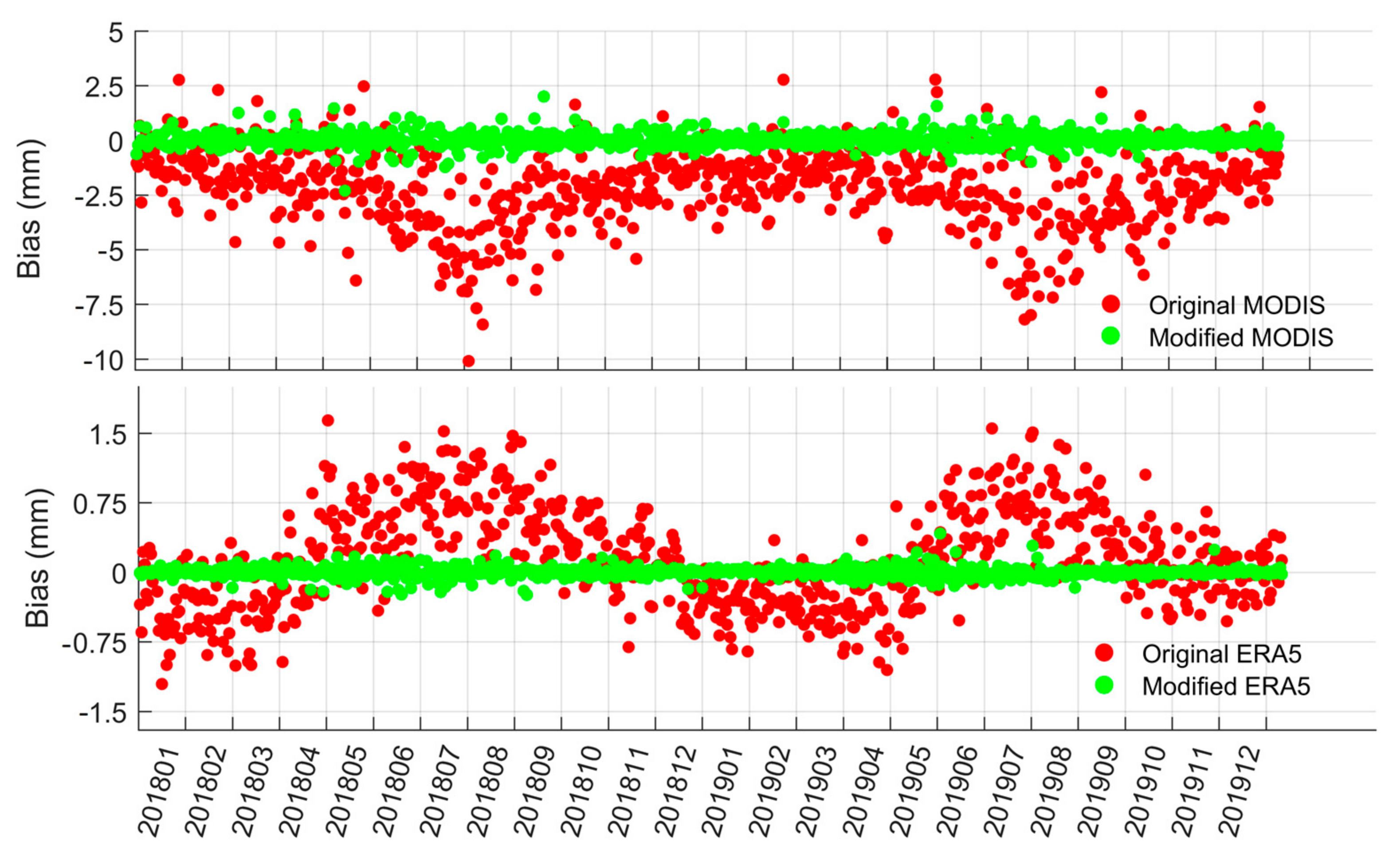
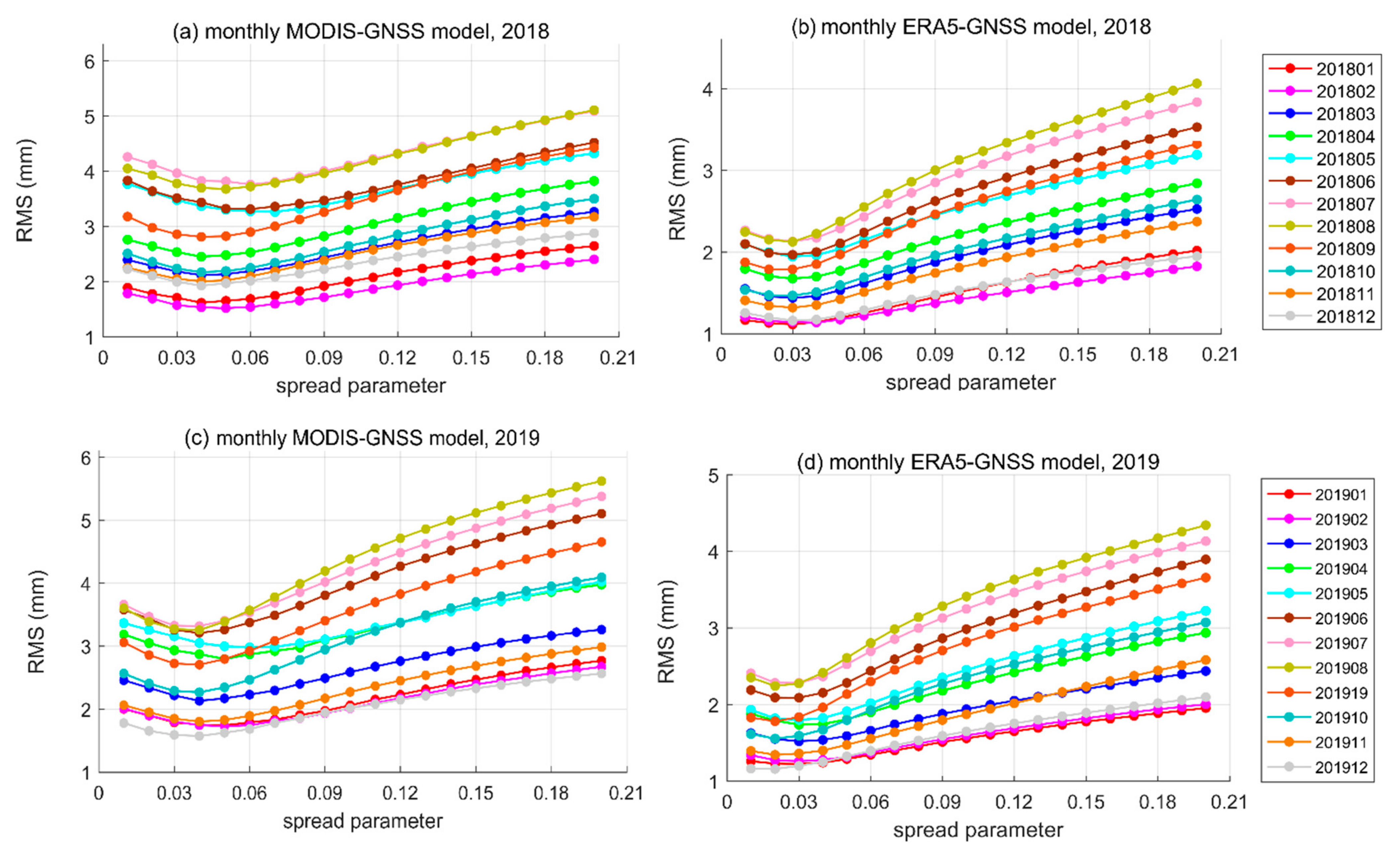
4.3. Model Performance at Monthly Timescale

From the above experiments, it is seen that the performance of the quarterly models is better than that of the annual models. It is easy to extend the models from quarterly to monthly.
Table 4 presents the overall performance of the monthly models with the optimal spread parameter given in Appendix B. The overall accuracy improvement in terms of RMS is 3.1 mm for MODIS PWV and 1.3 mm for ERA5 PWV, which is better than that by the quarterly models (2.5 mm for MODIS PWV and 1.1 mm for ERA5 PWV). The bias between MODIS (ERA5) PWV and GNSS PWV is reduced to 0 in the monthly models, which indicates that the systematic difference is eliminated.
Figure 5 shows the average bias, STD, RMS, and R of the monthly models in different months. For original MODIS PWV, the bias, STD and RMS are increased from winter to summer and then decreased from summer to winter. The original negative bias between GNSS PWV and MODIS PWV in all months indicates that MODIS PWV tends to be larger than GNSS PWV. The accuracy of MODIS PWV in terms of RMS of the monthly models in spring is improved by 2.0 mm for March, 2.4 mm for April, and 2.4 mm for May, respectively, which is better than that of quarterly models (1.8 mm). The results indicate that the MODIS-GNSS monthly models in the spring are better than the corresponding quarterly model. A similar conclusion can be made in other months. The R between MODIS PWV and GNSS PWV is obviously improved.
For ERA5 PWV, the original bias between ERA5 PWV and GNSS PWV shows that ERA5 PWV is larger than GNSS PWV in summer and autumn while smaller than GNSS PWV in spring and winter in China land region. The accuracy improvement in terms of RMS of the monthly models in spring is 0.9 mm for March, 1.1 mm for April, and 1.2 mm for May, respectively, which is not less than the corresponding quarterly model (0.9 mm). Similar conclusion can be made for other months. Those results show that the ERA5-GNSS monthly models could achieve better performance than the corresponding quarterly model. As shown in Figure 5h, the correlation coefficient R between ERA5 PWV and GNSS PWV is also increased.

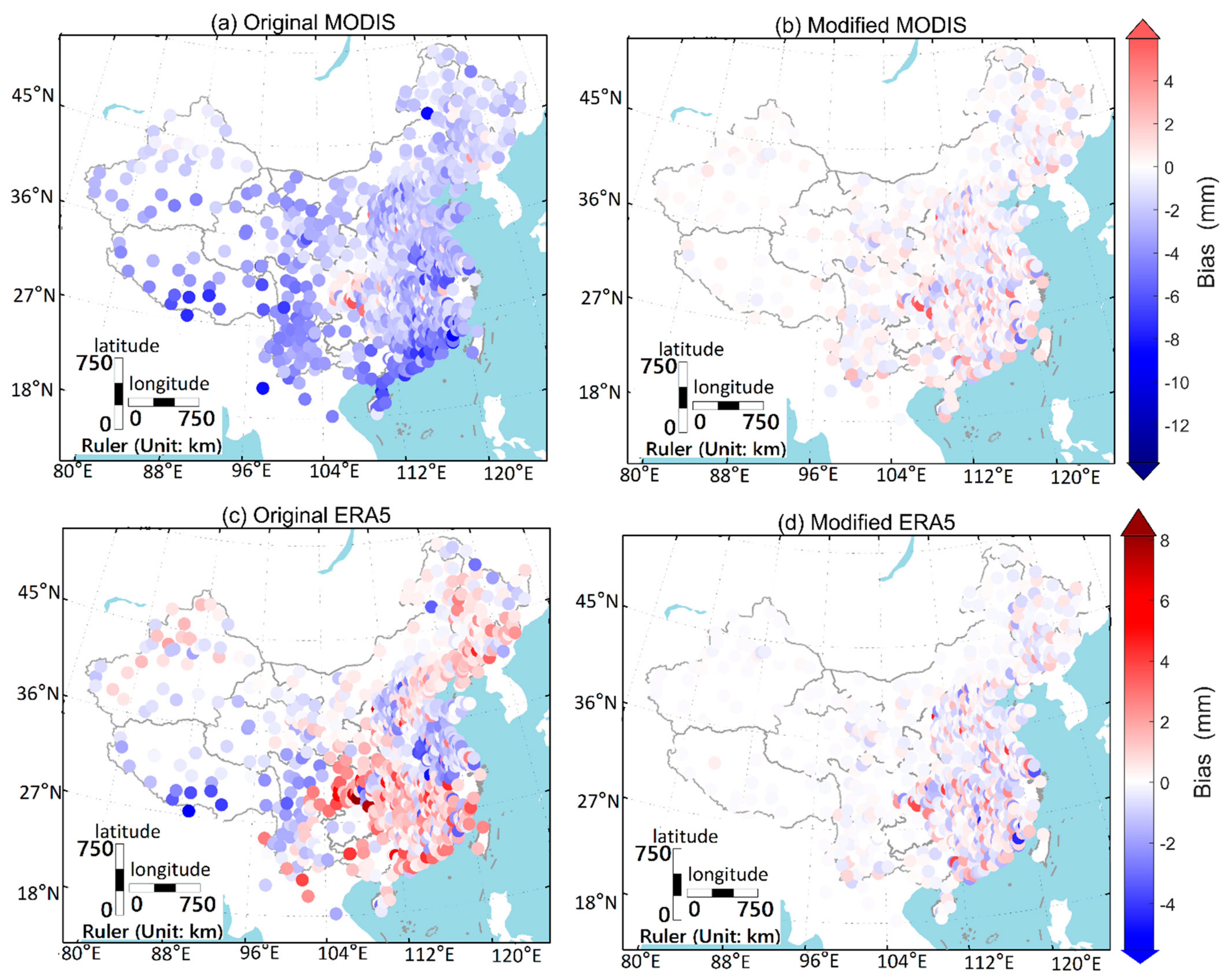
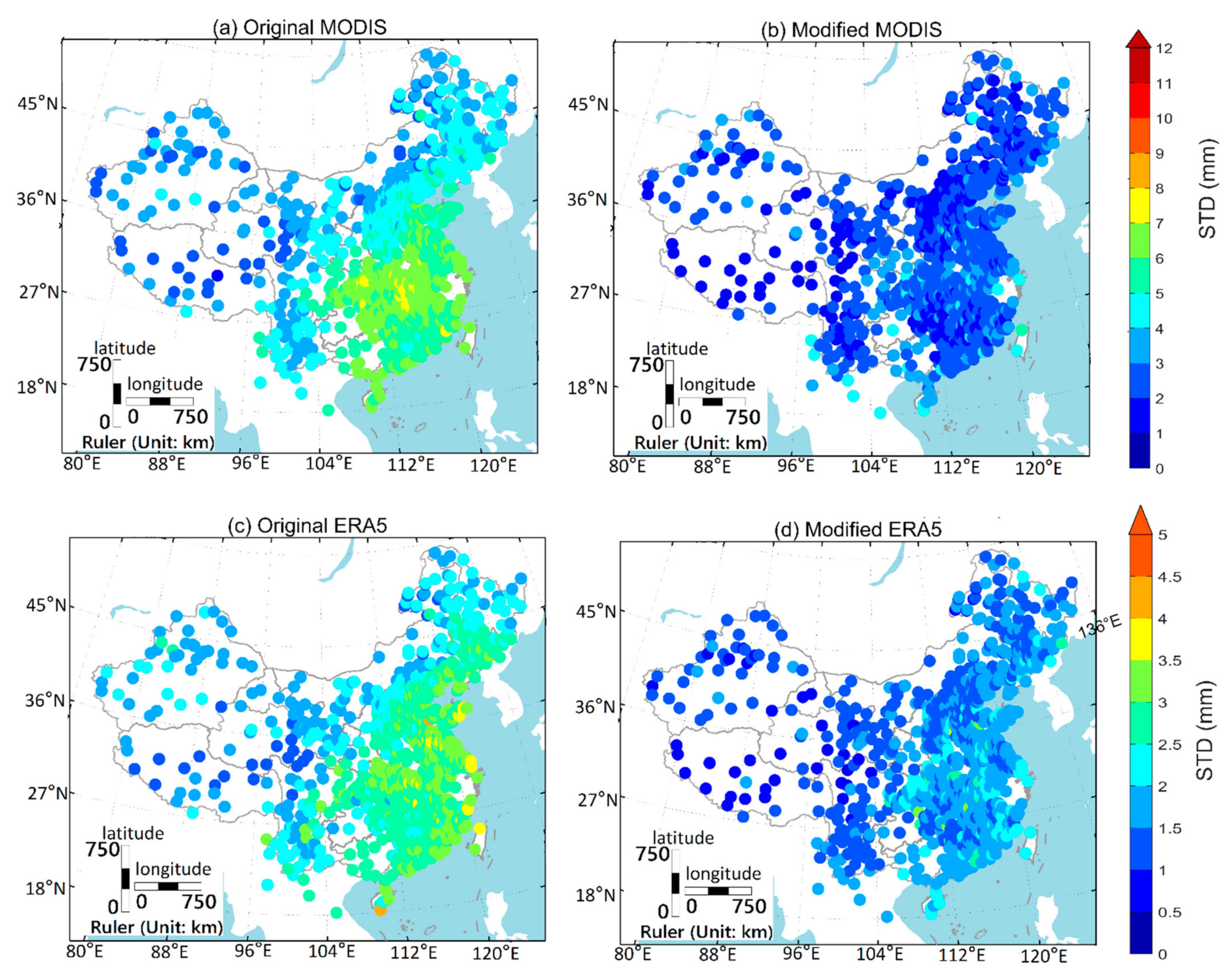
4.4. Generating PWV Products in the Research Area

From the above results, the monthly models achieved the best performance among the models of three timescales. Therefore, we use the monthly models to generate PWV products in the research area. The spatial resolution of the products is 1 km × 1 km in areas where MODIS PWV is present, and 0.25° × 0.25° in other areas. The temporal resolution is 1 day. Since the accuracy measured by RMS is 5–6 mm for the MODIS PWV and 3.0 mm for the ERA5 PWV in the research area while the accuracy of the fused PWV is better than 2.6 mm, apparently, the fusion provides a better PWV product for the research area.

5. Accuracy Analysis

To investigate the temporal variations of the model accuracy, we compute the daily bias, STD and RMS of the original MODIS (ERA5) PWV, and the modified MODIS (ERA5) PWV from the monthly models. The results are shown in Figure 6, Figure 7 and Figure 8. Figure 6 shows that the original MODIS PWV has overall negative biases with obvious temporal variations. The absolute values of the biases of the original MODIS PWV increased from January to July and then decreased from August to December. Most of the biases of the original ERA5 PWV are negative from December to April while positive in the rest months. There are also obvious temporal variations in the biases of the original ERA5 PWV. The biases of the modified MODIS PWV and the ERA5 PWV are close to 0 without noteworthy temporal fluctuations, which indicates the time-varying systematic biases between the MODIS (ERA5) PWV and the GNSS PWV are eliminated by the new methods.
Figure 7 shows the daily STDs of the original MODIS (ERA5) PWV and the modified MODIS (ERA5) PWV. It demonstrates that the STD of the original MODIS PWV has obvious temporal variations with an increase from January to July and a decrease from August to December. The modified MODIS PWV has apparently reduced STD whose temporal variations are also greatly weakened. The temporal pattern of STD of the ERA5 PWV is similar to that of the MODIS PWV.
Figure 8 shows the daily RMS of the original MODIS (ERA5) PWV and the modified MODIS (ERA5) PWV. The temporal patterns of the original MODIS (ERA5) PWV and the modified MODIS (ERA5) PWV are similar to that of STD. The temporal variations of RMS are greatly weakened for both MODIS PWV and ERA5 PWV after modeling.
To investigate the spatial variations of the model accuracy, we compute the bias, STD, and RMS of the original MODIS (ERA5) PWV and the modified MODIS (ERA5) PWV at individual GNSS stations. Figure 9 shows the biases of the original MODIS (ERA5) PWV and the modified MODIS (ERA5) PWV at the GNSS stations. It can be seen that the original MODIS PWV has negative biases at most stations. The biases are greater in the south and smaller in the north. These results suggest that the biases in the original MODIS PWV are uneven in the research area. Comparing Figure 9a,b, the biases between MODIS PWV and GNSS PWV are significantly decreased by the GRNN models, and their distribution becomes more even. Figure 9c shows that most of the biases of the original ERA5 PWV are positive in the south and northeast, and negative in the rest research area. Comparing Figure 9c,d, the biases of the modified ERA5 PWV are significantly reduced and distributed more evenly over the area.
Figure 10 shows the STDs of the original MODIS (ERA5) PWV and the modified MODIS (ERA5) PWV at individual stations. The STD of the original MODIS PWV is greater in the southeast while smaller in the northwest. Comparing Figure 10a,b, the STD of modified MODIS PWV is significantly reduced and the distribution is more even. A similar conclusion can be made for the modified ERA5 PWV.
Figure 11 shows the RMSs of the original MODIS (ERA5) PWV and the modified MODIS (ERA5) PWV at individual stations. Comparing Figure 11a,b, the RMS of MODIS PWV is reduced after modeling, especially for the stations in the southeast. We can find that the RMS of ERA5 PWV is also reduced after modeling by comparing Figure 11c,d.

6. Conclusions

Many scholars have used different methods to produce PWV products with high spatial resolution and improved accuracy in different regions. Zhang et al. [15] used a spherical cap harmonic model and Helmert variance component estimation method in North America. Zhao et al. [18] used a hybrid PWV fusion model in China. Alshawaf et al. [21] used a fixed-rank kriging method in Europe. All those methods could achieve better performance, but there are still some shortcomings. Some of the methods ignore the spatial or temporal variations in bias and only give a global bias for all observations. Some methods are based on the interpolation approach, which inevitably imposes some biases or inaccurate information due to the imperfect assumptions for the interpolation. In this study, we generate a PWV product in China area by fusing GNSS PWV, MODIS PWV, and ERA5 PWV in 2018 and 2019 through a generalized regression neural network. Models at annual, quarterly, and monthly timescales are constructed and performances are assessed to find out the best model for the research area. The results demonstrate that the monthly models achieve the best performance among the three timescales. Thus, we produce the fused PWV data by training and testing the GRNN models at a monthly timescale. Therefore, we have obtained a unified PWV product with a temporal resolution of 1 day and a spatial resolution better than 31 km. The bias, STD, and RMS of the modified MODIS PWV are 0.0 mm, 2.6 mm, and 2.6 mm. The percentage improvement is as high as 50% in terms of RMS. It becomes 0.0 mm, 1.7 mm, 1.7 mm for the modified ERA5 PWV and the percentage improvement is 40%. In this product, systematic differences between different PWV sources are almost diminished. Compared to the original MODIS (ERA5) PWV, the accuracy of the modified PWV is more even in space and time. With much improved quality, this PWV product can not only benefit the studies regarding water vapor circulation over China, but also serve in numerical weather forecasting.

Author Contributions

Conceptualization, Z.X. and B.Z.; methodology, Z.X. and B.Z.; validation, Z.X., X.S. and B.Z.; formal analysis, Z.X., B.Z. and J.S.; investigation, Z.X.; resources, X.S. and X.W.; data curation, Z.X.; writing—original draft preparation, Z.X.; writing—review and editing, B.Z. and J.S.; visualization, Z.X.; supervision, Z.X.; project administration, B.Z.; funding acquisition, B.Z. and X.S. All authors have read and agreed to the published version of the manuscript.

Funding

This work was jointly supported by the National key research and development program of China (2018YFC1506606); the key project of basic scientific research operating expenses of Chinese Academy of Meteorological Sciences(2019Z003); the National Natural Science Foundation of China (NNSFC), grant number 42074035 and 41874033; the Fundamental Research Funds for the Central Universities, grant number 2042020kf0009; and the China Postdoctoral Science Foundation, grant number 2018M630880 and 2019T120687.

Institutional Review Board Statement

Not applicable.

Informed Consent Statement

Not applicable.

Data Availability Statement

GNSS data from China Meteorological Administration (CMA) can be accessed from https://data.cma.cn/en/ (accessed on 25 April 2021), and GNSS data from the Crustal Movement Observation Network of China (CMONOC) is available through China Earthquake Administration. MODIS data used in this study is provided by NASA from the website at https://ladsweb.modaps.eosdis.nasa.gov/search/ (accessed on 25 April 2021). The reanalysis data, ERA5 products, is accessed from ECMWF at https://www.ecmwf.int/ (accessed on 25 April 2021).

Conflicts of Interest

The authors declare no conflict of interest.

Abbreviations

AbbreviationsFull Name
CMAChina Meteorological Administration
CMONOCCrustal Movement Observation Network of China
ECMWFEuropean Centre for Medium-Range Weather Forecasts
ERA5ECMWF ReAnalyses 5
GNSSGlobal Navigation Satellite System
GRNNGeneralized Regression Neural Network
IGSInternational GNSS Service
InSARInterferometric Synthetic Aperture Radar
MODISModerate-resolution Imaging Spectroradiometer
PPPPrecise Point Positioning
PWVprecipitable water vapor
Rcorrelation coefficient
RMSRoot Mean Square
STDSTandard Deviation
ZHDZenith Hydrostatic delay
ZTDZenith Total Delay
ZWDZenith Wet Delay

Appendix A. Radiosonde PWV Calculation Method

For a radiosonde station to be qualified as a reference station, it is required to be within 60 km in distance and 500 m in height of a GNSS station. The empirical formula in Equation (A1) is used to reduce the PWV value from a radiosonde station at height h2 to that at a GNSS station at height h1.
PWV h 1 = PWV h 2 exp ( h 1 h 2 2000 )
where PWV h 1 and PWV h 2 are the PWV values corresponding to the heights of h1 and h2 in m, respectively.
The transformational relation between ZWD and PWV can be found in Xiong et al. [11]. ZWD is related to water vapor pressure, temperature, and height difference between the two layers described in Formula (A2).
ZWD = P w × ( k 1 + k 2 T ) × h T
where P w is the water vapor pressure at each grid point in Pascal and can be obtained by Formula (A3), k1 = 2.21 × 10⁷ K/Pa, k2 = 3.73 × 10⁻³ K2/Pa, h is the height difference between the two layers in m, T is the temperature in K.
P w = RH × P s
where RH is the relative humidity. Ps is the saturated water vapor pressure which is related to the temperature and can be calculated by the Wexler formula [40,41].

Appendix B. The Model Performance against Spread Parameter Values

The spread parameter in a GRNN model has a great influence on the accuracy of the model, and it should be tuned to make the model perform well. In this study, a series of optional spread parameter values between 0.01 and 0.2 at a step of 0.01 is first set, and each value is tested. The testing results of different models, in terms of the Bias, STD, RMS and R, are shown below.
An appropriate spread parameter should not only make the modified accuracy as high as possible, but also make the fitting accuracy and modified accuracy comparable. The optimal spread parameter values are summarized in Table A1, and we use them to establish the models in this manuscript.
Figure A1. Annual model performance against spread parameter values.
Remotesensing 13 01720 g0a1
Figure A2. Quarterly model performance against spread parameter values.
Remotesensing 13 01720 g0a2
Figure A3. Monthly model performance against spread parameter values.
Remotesensing 13 01720 g0a3
Table A1. The optimal spread parameter values of different models.
Annual Models
yearMODIS-GNSSERA5-GNSSyearMODIS-GNSSERA5-GNSS
20180.050.0220190.050.02
Quarterly models
seasonMODIS-GNSSERA5-GNSSseasonMODIS-GNSSERA5-GNSS
spring 201803–2018050.060.03spring 201903–2019050.060.03
summer 201806–2018080.070.03summer 201906–2019080.050.03
autumn 201809–2018110.050.03autumn 201909–2019110.050.03
winter 201812–2019020.060.03
Monthly models
monthMODIS-GNSSERA5-GNSSmonthMODIS-GNSSERA5-GNSS
2018010.060.032019010.050.03
2018020.060.042019020.060.04
2018030.050.042019030.050.04
2018040.050.042019040.060.04
2018050.070.042019050.070.04
2018060.070.042019060.060.04
2018070.070.042019070.060.04
2018080.060.032019080.060.03
2018090.060.032019090.050.03
2018100.050.042019100.050.03
2018110.060.042019110.050.02
2018120.060.032019120.050.03

References

  1. Huang, Q.; Zhang, Q.; Singh, V.P.; Shi, P.; Zheng, Y. Variations of dryness/wetness across China: Changing properties, drought risks, and causes. Glob. Planet. Chang. 2017, 155, 1–12. [Google Scholar] [CrossRef]
  2. Wang, P.; Wu, X.; Hao, Y.; Wu, C.; Zhang, J. Is Southwest China drying or wetting? Spatiotemporal patterns and potential causes. Theor. Appl. Climatol. 2020, 139, 1–15. [Google Scholar] [CrossRef]
  3. Li, Z.; Muller, J.P.; Cross, P.; Fielding, E.J. Interferometric synthetic aperture radar (InSAR) atmospheric correction: GPS, Moderate Resolution Imaging Spectroradiometer (MODIS), and InSAR integration. J. Geophys Res. Solid Earth. 2005, 110. [Google Scholar] [CrossRef]
  4. Ningombam, S.S.; Jade, S.; Shrungeshwara, T.S.; Song, H.J. Validation of water vapor retrieval from Moderate Resolution Imaging Spectro-radiometer (MODIS) in near infrared channels using GPS data over IAO-Hanle, in the trans-Himalayan region. J. Atmos. Sol. Terr. Phys. 2016, 137, 76–85. [Google Scholar] [CrossRef]
  5. Khaniani, A.S.; Nikraftar, Z.; Zakeri, S. Evaluation of MODIS Near-IR water vapor product over Iran using ground-based GPS measurements. Atmos. Res. 2020, 231, 104657. [Google Scholar] [CrossRef]
  6. Bevis, M.; Businger, S.; Herring, T.A.; Rocken, C.; Anthes, R.A.; Ware, R.H. GPS meteorology: Remote sensing of atmospheric water vapor using the Global Positioning System. J. Geophys. Res. Atmos. 1992, 97, 15787–15801. [Google Scholar] [CrossRef]
  7. Bevis, M.; Businger, S.; Chiswell, S.; Herring, T.A.; Anthes, R.A.; Rocken, C.; Ware, R.H. GPS meteorology: Mapping zenith wet delays onto precipitable water. J. Appl. Meteorol. 1994, 33, 379–386. [Google Scholar] [CrossRef]
  8. Yao, Y.; Shan, L.; Zhao, Q. Establishing a method of short-term rainfall forecasting based on GNSS-derived PWV and its application. Sci. Rep. 2017, 7, 1–11. [Google Scholar] [CrossRef]
  9. Bock, O.; Nuret, M. Verification of NWP model analyses and radiosonde humidity data with GPS precipitable water vapor estimates during AMMA. Weather Forecast. 2009, 24, 1085–1101. [Google Scholar] [CrossRef]
  10. Zhang, Q.; Ye, J.; Zhang, S.; Han, F. Precipitable water vapor retrieval and analysis by multiple data sources: Ground-based GNSS, radio occultation, radiosonde, microwave satellite, and NWP reanalysis data. J. Sens. 2018, 2018, 3428303. [Google Scholar] [CrossRef]
  11. Xiong, Z.; Sang, J.; Sun, X.; Zhang, B.; Li, J. Comparisons of Performance Using Data Assimilation and Data Fusion Approaches in Acquiring Precipitable Water Vapor: A Case Study of a Western United States of America Area. Water 2020, 12, 2943. [Google Scholar] [CrossRef]
  12. Liu, H.; Tang, S.; Zhang, S.; Hu, J. Evaluation of MODIS water vapour products over China using radiosonde data. Int. J. Remote Sens. 2015, 36, 680–690. [Google Scholar] [CrossRef]
  13. Gui, K.; Che, H.; Chen, Q.; Zeng, Z.; Liu, H.; Wang, Y.; Zheng, Y.; Sun, T.; Liao, T.; Wang, H.; et al. Evaluation of radiosonde, MODIS-NIR-Clear, and AERONET precipitable water vapor using IGS ground-based GPS measurements over China. Atmos. Res. 2017, 197, 461–473. [Google Scholar] [CrossRef]
  14. Li, Z. Production of Regional 1 km × 1 km Water Vapor Fields through the Integration of GPS and MODIS Data. In Proceedings of the 17th International Technical Meeting of the Satellite Division of the Institute of Navigation (ION GNSS 2004), Long Beach, CA, USA, 21–24 September 2004; pp. 2396–2403. [Google Scholar]
  15. Zhang, B.; Yao, Y.; Xin, L.; Xu, X. Precipitable water vapor fusion: An approach based on spherical cap harmonic analysis and Helmert variance component estimation. J. Geod. 2019, 93, 2605–2620. [Google Scholar] [CrossRef]
  16. Rocken, C.; Ware, R.; Van Hove, T.; Solheim, F.; Alber, C.; Johnson, J.; Bevis, M.; Businger, S. Sensing atmospheric water vapor with the Global Positioning System. Geophys. Res. Lett. 1993, 20, 2631–2634. [Google Scholar] [CrossRef] [Green Version]
  17. Tregoning, P.; Boers, R.; O’Brien, D.; Hendy, M. Accuracy of absolute precipitable water vapor estimates from GPS observations. J. Geophys. Res. Atmos. 1998, 103, 28701–28710. [Google Scholar] [CrossRef]
  18. Zhao, Q.; Du, Z.; Yao, W.; Yao, Y. Hybrid precipitable water vapor fusion model in China. J. Atmos. Sol. Terr. Phys. 2020, 208, 105387. [Google Scholar] [CrossRef]
  19. Lindenbergh, R.; Van der Marel, H.; Keshin, M.; De Haan, S. Validating time series of a combined GPS and MERIS Integrated Water Vapor product. In Proceedings of the 2nd MERIS/(A) ATSR User Workshop, Frascati, Italy, 22–26 September 2008; ESA/ESRIN: Frascati, Italy, 2009. NB: Small correction applied wrt Proceedings version. [Google Scholar]
  20. Alshawaf, F.; Hinz, S.; Mayer, M.; Meyer, F.J. Constructing accurate maps of atmospheric water vapor by combining interferometric synthetic aperture radar and GNSS observations. J. Geophys. Res. Atmos. 2015, 120, 1391–1403. [Google Scholar] [CrossRef]
  21. Alshawaf, F.; Fersch, B.; Hinz, S.; Kunstmann, H.; Mayer, M.; Meyer, F.J. Water vapor mapping by fusing InSAR and GNSS remote sensing data and atmospheric simulations. Hydrol. Earth Syst. Sci. 2015, 19, 4747–4764. [Google Scholar] [CrossRef] [Green Version]
  22. Li, X.; Long, D. An improvement in accuracy and spatiotemporal continuity of the MODIS precipitable water vapor product based on a data fusion approach. Remote Sens. Environ. 2020, 248, 111966. [Google Scholar] [CrossRef]
  23. Bai, J.; Lou, Y.; Zhang, W.; Zhou, Y.; Zhang, Z.; Shi, C. Assessment and calibration of MODIS precipitable water vapor products based on GPS network over China. Atmos. Res. 2021, 254, 105504. [Google Scholar] [CrossRef]
  24. Zhang, B.; Yao, Y. Precipitable water vapor fusion based on a generalized regression neural network. J. Geod. 2021, 95, 1–14. [Google Scholar] [CrossRef]
  25. Liang, H.; Cao, Y.; Wan, X.; Xu, Z.; Wang, H.; Hu, H. Meteorological applications of precipitable water vapor measurements retrieved by the national GNSS network of China. Geod. Geodyn. 2015, 6, 135–142. [Google Scholar] [CrossRef] [Green Version]
  26. Yao, Y.; Xu, X.; Xu, C.; Peng, W.; Wan, Y. Establishment of a real-time local tropospheric fusion model. Remote Sens. 2019, 11, 1321. [Google Scholar] [CrossRef] [Green Version]
  27. Kouba, J.; Héroux, P. Precise point positioning using IGS orbit and clock products. GPS Solut. 2001, 5, 12–28. [Google Scholar] [CrossRef]
  28. Dach, R.; Schaer, S.; Arnold, D.; Kalarus, S.; Prange, L.; Stebler, P.; Villiger, A.; Jäggi, A. CODE Final Product Series for the IGS; Astronomical Institute, University of Bern: Bern, Switzerland, 2020. [Google Scholar] [CrossRef]
  29. Saastamoinen, J. Atmospheric correction for the troposphere and stratosphere in radio ranging satellites. Geophys. Monogr. Ser. 1972, 15, 247–251. [Google Scholar]
  30. Hersbach, H.; Bell, B.; Berrisford, P.; Hirahara, S.; Horányi, A.; Muñoz-Sabater, J.; Nicolas, J.; Peubey, C.; Radu, R.; Schepers, D.; et al. The ERA5 global reanalysis. Q. J. R. Meteorol. Soc. 2020, 146, 1999–2049. [Google Scholar] [CrossRef]
  31. Reuter, H.I.; Nelson, A.; Jarvis, A. An evaluation of void-filling interpolation methods for SRTM data. Int. J. Geogr. Inf. Sci. 2007, 21, 983–1008. [Google Scholar] [CrossRef]
  32. Jarvis, A.; Reuter, H.I.; Nelson, A.; Guevara, E. Hole-Filled Seamless SRTM Data V4, International Centre for Tropical Agriculture (CIAT). 2008. Available online: http://srtm.csi.cgiar.org (accessed on 20 April 2020).
  33. Prasad, A.K.; Singh, R.P. Validation of MODIS Terra, AIRS, NCEP/DOE AMIP-II Reanalysis-2, and AERONET Sun photometer derived integrated precipitable water vapor using ground-based GPS receivers over India. J. Geophys. Res. Atmos. 2009, 114. [Google Scholar] [CrossRef] [Green Version]
  34. Roman, J.; Knuteson, R.; August, T.; Hultberg, T.; Ackerman, S.; Revercomb, H. A global assessment of NASA AIRS v6 and EUMETSAT IASI v6 precipitable water vapor using ground-based GPS SuomiNet stations. J. Geophys. Res. Atmos. 2016, 121, 8925–8948. [Google Scholar] [CrossRef]
  35. Li, J.; Zhang, B.; Yao, Y.; Liu, L.; Sun, Z.; Yan, X. A Refined Regional Model for Estimating Pressure, Temperature, and Water Vapor Pressure for Geodetic Applications in China. Remote Sens. 2020, 12, 1713. [Google Scholar] [CrossRef]
  36. Specht, D.F. A general regression neural network. IEEE Trans. Neural Netw. 1991, 2, 568–576. [Google Scholar] [CrossRef] [PubMed] [Green Version]
  37. Polat, K.; Güneş, S. Classification of epileptiform EEG using a hybrid system based on decision tree classifier and fast Fourier transform. Appl. Math. Comput. 2007, 187, 1017–1026. [Google Scholar] [CrossRef]
  38. Zhang, H.; Yang, S.; Guo, L.; Zhao, Y.; Shao, F.; Chen, F. Comparisons of isomiR patterns and classification performance using the rank-based MANOVA and 10-fold cross-validation. Gene 2015, 569, 21–26. [Google Scholar] [CrossRef]
  39. Tandon, S.; Tripathi, S.; Saraswat, P.; Dabas, C. Bitcoin Price Forecasting using LSTM and 10-Fold Cross validation. In Proceedings of the 2019 International Conference on Signal Processing and Communication (ICSC), Noida, India, 7–9 March 2019; pp. 323–328. [Google Scholar]
  40. Wexler, A. Vapor pressure formulation for water in range 0 to 100 °C. A revision. J. Res. Natl. Bur. Stand. A 1976, 80, 775–785. [Google Scholar] [CrossRef]
  41. Wexler, A. Vapor pressure formulation for ice. J. Res. Natl. Bur. Stand. A 1977, 81, 5–20. [Google Scholar] [CrossRef]
Figure 1. (a) Research area and the distribution of GNSS stations and Radiosonde stations; (b) the localization of study area (showing as red area) at a global scale.
Remotesensing 13 01720 g001
Figure 2. MODIS (ERA5)-GNSS PWV GRNN fusion model.
Remotesensing 13 01720 g002
Figure 3. Scatter plots of the modified MODIS PWV against observed (GNSS) PWV.
Remotesensing 13 01720 g003
Figure 4. Accuracy information of the quarterly models in different seasons. (a) Bias of the MODIS-GNSS model; (b) STD of the MODIS-GNSS model; (c) RMS of the MODIS-GNSS model; (d) R of the MODIS-GNSS model; (e) Bias of the ERA5-GNSS model; (f) STD of the ERA5-GNSS model; (g) RMS of the ERA5-GNSS model; (h) R of the ERA5-GNSS model.
Remotesensing 13 01720 g004
Figure 5. Accuracy information of the monthly models in different months. (a) Bias of the MODIS-GNSS model; (b) STD of the MODIS-GNSS model; (c) RMS of the MODIS-GNSS model; (d) R of the MODIS-GNSS model; (e) Bias of the ERA5-GNSS model; (f) STD of the ERA5-GNSS model; (g) RMS of the ERA5-GNSS model; (h) R of the ERA5-GNSS model.
Remotesensing 13 01720 g005
Figure 6. Daily PWV biases of the original MODIS (ERA5) PWV and the modified MODIS (ERA5) PWV.
Remotesensing 13 01720 g006
Figure 7. Daily PWV STD of the original MODIS (ERA5) PWV and the modified MODIS (ERA5) PWV.
Remotesensing 13 01720 g007
Figure 8. Daily PWV RMS of the original MODIS (ERA5) PWV and the modified MODIS (ERA5) PWV.
Remotesensing 13 01720 g008
Figure 9. PWV biases at individual stations of the original MODIS (ERA5) PWV and the modified MODIS (ERA5) PWV.
Remotesensing 13 01720 g009
Figure 10. PWV STD at individual stations of the original MODIS (ERA5) PWV and the modified MODIS (ERA5) PWV.
Remotesensing 13 01720 g010
Figure 11. PWV RMS at individual stations of the original MODIS (ERA5) PWV and the modified MODIS (ERA5) PWV.
Remotesensing 13 01720 g011
Table 1. Average accuracy of data pairs after removing outliers.
Unit: mmBiasSTDRMSR
MODIS-GNSS−2.35.25.70.96
ERA5-GNSS0.23.03.00.99
Note: Biases are computed based on GNSS PWV minus MODIS (ERA5) PWV in this manuscript.
Table 2. Model performance based on annual samples.
Unit: mm BiasSTDRMSR
MODIS-GNSSModified0.13.83.80.98
Fitting0.03.43.40.98
ERA5-GNSSModified0.02.02.00.99
Fitting0.01.51.51.00
Table 3. Model performance based on quarterly samples.
Unit: mmAccuracyBiasSTDRMSR
MODIS-GNSSModified0.1 3.2 3.2 0.98
Fitting0.0 2.6 2.6 0.99
ERA5-GNSSModified0.0 1.9 1.9 0.99
Fitting0.0 1.4 1.4 1.00
Table 4. Model performance based on monthly samples.
Unit: mmAccuracyBiasSTDRMSR
MODIS-GNSSModified0.0 2.6 2.6 0.98
Fitting0.0 1.7 1.7 0.99
ERA5-GNSSModified0.0 1.7 1.7 0.99
Fitting0.0 1.2 1.2 1.00
Publisher’s Note: MDPI stays neutral with regard to jurisdictional claims in published maps and institutional affiliations.

