Robust Multipath-Assisted SLAM with Unknown Process Noise and Clutter Intensity

Abstract

In multipath-assisted simultaneous localization and mapping (SLAM), the geometric association of specular multipath components based on radio signals with environmental features is used to simultaneously localize user equipment and map the environment. We must contend with two notable model parameter uncertainties in multipath-assisted SLAM: process noise and clutter intensity. Knowledge of these two parameters is critically important to multipath-assisted SLAM, the uncertainty of which will seriously affect the SLAM accuracy. Conventional multipath-assisted SLAM algorithms generally regard these model parameters as fixed and known, which cannot meet the challenges presented in complicated environments. We address this challenge by improving the belief propagation (BP)-based SLAM algorithm and proposing a robust multipath-assisted SLAM algorithm that can accommodate model mismatch in process noise and clutter intensity. Specifically, we describe the evolution of the process noise variance and clutter intensity via Markov chain models and integrate them into the factor graph representing the Bayesian model of the multipath-assisted SLAM. Then, the BP message passing algorithm is leveraged to calculate the marginal posterior distributions of the user equipment, environmental features and unknown model parameters to achieve the goals of simultaneous localization and mapping, as well as adaptively learning the process noise variance and clutter intensity. Finally, the simulation results demonstrate that the proposed approach is robust against the uncertainty of the process noise and clutter intensity and shows excellent performances in challenging indoor environments.

1. Introduction

Simultaneous localization and mapping (SLAM) [1,2] aims to estimate the time-varying position of the mobile agent when it is moving in an unknown environment and build a map of the surroundings from measurements provided by sensors. SLAM is significant in many fields, such as robotics [3], autonomous driving [4], and situation awareness [5]. In multipath-assisted methods [6,7,8,9,10], the relation between multipath components (MPCs) of radio signals and local geometry is used to turn the multipath propagation from an error source to an advantage that can improve the positioning accuracy. Recently, multipath-assisted SLAM, a combination of the two, has attracted considerable attention from scholars and has been applied in the field of indoor positioning [11,12,13,14,15,16].

Instead of mapping the environment in conventional SLAMs, the map in multipath-assisted SLAM is represented by an unknown number of features with unknown spatial positions. Features denote the physical transmitters (PTs) and virtual transmitters (VTs) in the environment. Radio signals are transmitted from base stations (PTs) to the user equipment (UE). Specular MPCs in the multipath radio channel are described by VTs, which are mirror images of the PTs. Due to the introduction of VTs, specular MPCs can be interpreted as line-of-sight (LOS) signals from the VTs, which can increase the number of transmitters involved in positioning and even realize localization in the case of insufficient PTs. Multipath-assisted SLAM detects the VTs associated with the PTs and estimates their positions as well as the trajectory of the UE. Multipath-assisted SLAM can cope with harsh multipath channel conditions and realize positioning and mapping without knowing the prior position of the PTs or without having a sufficient number of PTs, which greatly improves the accuracy and robustness of indoor positioning [17,18,19,20,21].

The data association (DA) between measurements and PTs or VTs is unknown, and measurements will be affected by noise, false alarms and missed detections, which makes the multipath-assisted SLAM complex. A multipath-assisted SLAM algorithm called Channel-SLAM was proposed in [22]. Channel-SLAM is based on a recursive Bayesian filter and can realize SLAM only with the prior position of the PT and the initial position and orientation of the UE. However, Channel-SLAM does not consider the DA uncertainty. Channel-SLAM is extended in [23] by adding a multiple hypothesis tracking (MHT)-based DA algorithm, which enables Channel-SLAM to associate the reappearing MPCs with corresponding VTs. Simulation results demonstrate that the improved Channel-SLAM algorithm has higher positioning reliability and lower computational complexity than the original method. A multipath-assisted SLAM algorithm called BP-SLAM based on belief propagation (BP) [24] was proposed in [25]. The approach jointly realizes the probabilistic DA and the estimation of UE positions and feature positions in the environment map. Simulation results demonstrate that BP-SLAM has lower complexity and higher scalability than other state-of-the-art SLAM algorithms and has higher positioning and mapping accuracy in the case of measurements containing false alarms and missed detections.

Furthermore, unknown and time-varying model parameters also complicate multipath-assisted SLAM. For example, the detection probability describes the possibility of PTs or VTs being detected by the UE. In practice, due to the influence of electromagnetic interference and surrounding environments, the detection probability is usually variable. However, the influence of the detection probability was not considered or simply considered to be fixed and known in [22,23,24,25]. Adaptive algorithms of the time-varying detection probability-based BP-SLAM algorithm were proposed in [26,27,28]. In [26], the detection probability was considered to be a discrete random variable with the value taking from a finite set. Then, the evolution of the detection probability was integrated into the multipath-assisted SLAM Bayesian model as an independent variable node. Thus, the algorithm can realize the online adaptive adjustment of the detection probability. In [27,28], the detection probability was expressed as a function of the MPC amplitude, and improved BP-SLAM algorithms were proposed, which leveraged MPC amplitude information to adaptively adjust the detection probability.

In multipath-assisted SLAM, we have to address the uncertainty of two important model parameters, process noise and clutter intensity, in addition to the detection probability. The change in process noise is mainly reflected in the change in UE dynamic models. Maneuvering or sudden acceleration and turning may cause process model uncertainties in UEs. Clutter represents spurious measurements that do not come from any transmitter (PTs or VTs). Clutter intensity is used to describe the amount of clutter in the environment. To the best of the authors’ knowledge, none of the multipath-assisted SLAM algorithms consider the uncertainty of process noise and clutter intensity at present. However, in the field of multitarget tracking (MTT) [29], which is closely related to feature-based SLAM, some algorithms are proposed with the condition that these two model parameters are unknown. In [30,31], clutter was regarded as measurements generated by incorrect targets. By distinguishing between correct and incorrect targets, the probability hypothesis density (PHD) filter, the cardinalized PHD (CPHD) filter, and the multi-Bernoulli filter were developed to independently estimate the clutter intensity in the environment. The conventional PHD filter and CPHD filter were extended in [32] to include estimation of the time-varying target birth intensity. In [33], an adaptive MTT algorithm based on the factor graph and the sum product algorithm [34] was proposed. The algorithm can be applied to complex scenes where the target dynamic model and detection probability change at the same time.

Most of the existing multipath-assisted SLAM algorithms regard the process noise and clutter intensity as known and fixed. However, in practical applications, the dynamic model of UEs cannot remain invariable all the time, and the process noise of UEs may change at any time. Clutter environments are often complicated due to the influence of electromagnetic interference, signal scattering and diffraction; hence, it is difficult to match the assumption of known process noise and clutter intensity with reality. Significant mismatches in the process and clutter model parameters seriously affect the SLAM accuracy, and even the estimation results diverge. Therefore, it is of critical importance to study the robust multipath-assisted SLAM algorithm when the process and clutter model parameters are unknown. Based on the framework of the BP-SLAM algorithm, in this paper, we propose a robust multipath-assisted SLAM algorithm, which can address the uncertainties of process and clutter model parameters in multipath-assisted SLAM. First, the UE state is extended to an augmented state including the process noise, and the evolution of the augmented state is described by new prediction and update rules compared to the conventional BP-SLAM algorithm. Second, we add a new variable to represent the clutter intensity in the Bayesian model of BP-SLAM and describe the evolution of the clutter intensity via a Markov chain model. Finally, we integrate the augmented state of the UE and the new variable node into a factor graph representing the Bayesian model of BP-SLAM and use the BP message passing algorithm to calculate marginal posterior distributions of the process noise, the clutter intensity, the UE and other features to realize the online adjustment of the process noise and the clutter intensity in multipath-assisted SLAM. The simulation results demonstrate that the proposed algorithm can adaptively learn the process noise and clutter intensity for SLAM, improving the robustness of the multipath-assisted SLAM system.

The remainder of this paper is organized as follows: Section 2 provides the environment map and the signal model. Section 3 describes the system model with unknown process noise and clutter intensity. Moreover, our robust multipath-assisted SLAM algorithm is proposed in Section 4. Then, the simulation results are reported in Section 5. Finally, Section 6 contains the conclusion of the paper.

2. Environment Map and Signal Model

Multipath-assisted SLAM combines the geometric parameters (delays, angles of arrival (AOAs) and angles of departure (AODs)) of the LOS signal in received radio signals with the geometric parameters of specular MPCs to localize the UE and build the environment map. These parameters are obtained according to the relationship between the positions of the UE and the PTs or VTs. The VT positions are mirror images of the PT positions with respect to the reflection surface. From the UE side, the reflected and virtual propagation paths originating from the VTs have the same AOA and delay; hence, the reflected path can be described as a LOS path between the VT and the UE. Regardless of how the UE moves, the VTs will remain static as long as the PTs are static. As an example, Figure 1 depicts an indoor environment map containing two PTs and some of the corresponding VTs. The red solid circle and the blue solid box denote PT1 and PT2 at ${\mathit{a}}_1^{(1)}$ and ${\mathit{a}}_1^{(2)}$, respectively. The gray lines represent the doors, windows and walls in the room. They all have smooth surfaces that can reflect the radio signals from the PTs. The red hollow circles and blue hollow boxes represent the corresponding VTs, which are mirror images of PT1 and PT2. The green dot is the estimated position of the UE at ${\mathit{u}}_n$, while the magenta line denotes the real trajectory of the UE.

We consider an environment map with one UE and J PTs. The UE position is unknown and time-varying, which is denoted by ${\mathit{u}}_n\in {ℝ}^2$, while the PT positions ${\mathit{a}}_1^{(j)}\in {ℝ}^2,j\in \left\{1,\dots ,J\right\}$ may be unknown, where the number of PT J is supposed to be known. Assume that there are $L_n^{(j)}-1$ VTs associated with the jth PT and that their positions are unknown and represented by ${\mathit{a}}_l^{(j)}\in {ℝ}^2,l\in \left\{2,\dots ,L_n^{(j)}\right\}$. PTs and VTs are features of the environmental map, and their number is unknown and varies with the UE position. At each discrete time n, the radio signal $s(t)$ is transmitted from the jth PT to the mobile UE, and the received signal of the UE can be expressed as [17]

$$s_{\mathrm{RX},n}(t)={\displaystyle \sum _{l=1}^{L_n^{(j)}}{\partial }_{l,n}^{(j)}s(t-{\tau }_{l,n}^{(j)})+g_n^{(j)}(t)+{\omega }_{\mathrm{GWN}}(t)}$$

(1)

The first term on the right in Equation (1) describes $L_n^{(j)}$ specular MPCs with complex amplitude ${\partial }_{l,n}^{(j)}$ and time delay ${\tau }_{l,n}^{(j)}$, where $l\in \left\{1,\dots ,L_n^{(j)}\right\}$. These MPCs correspond to the features (PTs and VTs) of the environment. The delay ${\tau }_{l,n}^{(j)}$ corresponds to the distance between the UE and the jth PT ($l=1$) or the associated VTs ($l\in \left\{2,\dots ,L_n^{(j)}\right\}$); thus, we have ${\tau }_{l,n}^{(j)}=\Vert {\mathit{u}}_n-{\mathit{a}}_l^{(j)}\Vert /c$, where c is the speed of light. Furthermore, $g_n^{(j)}(t)$ in (1) denotes the diffuse MPCs, which is regarded as interference. Finally, ${\omega }_{\mathrm{GWN}}(t)$ represents additive white Gaussian noise.

At each time n, the radio channel estimator [35] processes the signal $s_{\mathrm{RX},n}(t)$ received by the UE to obtain $M_n^{(j)}$ delay estimations of MPCs ${\widehat{\tau }}_{m,n}^{(j)},m\in {ℳ}_n^{(j)}=\left\{1,\dots ,M_n^{(j)}\right\}$. The relation between the number of MPC delay estimations $M_n^{(j)}$ and the number of specular MPCs $L_n^{(j)}$ is as follows: on the one hand, some specular MPCs are unlikely to be detected by the radio channel estimator without generating delay estimations; on the other hand, some of the delay estimations cannot correspond to any specular MPCs. Therefore, there is no exact equality between $M_n^{(j)}$ and $L_n^{(j)}$, and $M_n^{(j)}$ mainly depends on the UE position ${\mathit{u}}_n$ and the environment. The estimated distances $z_{m,n}^{(j)}$, $m\in \left\{1,\dots ,M_n^{(j)}\right\}$ of the mth MPC of PT j are obtained by multiplying the delay estimation ${\widehat{\tau }}_{m,n}^{(j)}$ with the speed of light c, which are the measurements of the proposed algorithm used in this paper. For convenience, we define the stacked vectors of $z_{m,n}^{(j)}$, ${\mathit{z}}_n^{(j)}\triangleq {\left[z_{1,n}^{(j)}\cdots z_{M_n^{(j)},n}^{(j)}\right]}^{\mathrm{T}}$, ${\mathit{z}}_n\triangleq {\left[{\mathit{z}}_n^{(1)\mathrm{T}}\cdots {\mathit{z}}_n^{(J)\mathrm{T}}\right]}^{\mathrm{T}}$ and $\mathit{z}\triangleq {\left[{\mathit{z}}_1^{\mathrm{T}}\cdots {\mathit{z}}_n^{\mathrm{T}}\right]}^{\mathrm{T}}$ and the stacked vectors of $M_n^{(j)}$, ${\mathit{m}}_n\triangleq {\left[M_n^{(1)}\cdots M_n^{(J)}\right]}^{\mathrm{T}}$ and $\mathit{m}={\left[{\mathit{m}}_1^{\mathrm{T}}\cdots {\mathit{m}}_n^{\mathrm{T}}\right]}^{\mathrm{T}}$.

3. System Model with Unknown Process Noise and Clutter Intensity

3.1. UE State and PF States

The UE state at time n is ${\tilde{\mathit{x}}}_n\triangleq {\left[\begin{array}{cc}{\mathit{u}}_n^{\mathrm{T}}& {\mathit{v}}_n^{\mathrm{T}}\end{array}\right]}^{\mathrm{T}}$ and ${\mathit{v}}_n$ denotes the UE velocity vector. Potential features (PFs) are used to describe the features in the environment map (PTs and VTs) because the number of VTs is unknown and time-varying. PFs are indexed via (j, k), where $j\in \left\{1,\dots ,J\right\}$ and $k\in {\mathcal{K}}_n^{(j)}\triangleq \left\{1,\dots ,K_n^{(j)}\right\}$ (which implies that there are $K_n^{(j)}$ PFs for each PT j). Note that the set of PFs includes the PT itself, and the number of PFs is unknown and varies with the UE position. We use the indicator variable $e_{k,n}^{(j)}\in \left\{0,1\right\}$ to indicate whether PFs truly exist, where $e_{k,n}^{(j)}=1$ means that PF (j, k) exists at time n, and vice versa. The indicator variable $e_{k,n}^{(j)}$ is used to estimate the existence probability of PFs, which will be introduced in Section 4.1. The state of the PF (j, k) at time n is represented as an augmented state including the indicator variable $e_{k,n}^{(j)}$, i.e., ${\mathit{y}}_{k,n}^{(j)}={\left[\begin{array}{cc}{\mathit{a}}_{k,n}^{(j)}{}^{\mathrm{T}}& e_{k,n}^{(j)}\end{array}\right]}^{\mathrm{T}}$, where ${\mathit{a}}_{k,n}^{(j)}$ denotes the PF (j, k) position. We also define the stacked vectors of ${\mathit{y}}_{k,n}^{(j)}$, i.e., ${\mathit{y}}_n^{(j)}={\left[{\mathit{y}}_{1,n}^{(j)}{}^{\mathrm{T}}\dots {\mathit{y}}_{K_n^{(j)},n}^{(j)\mathrm{T}}\right]}^{\mathrm{T}}$, ${\mathit{y}}_n={\left[{\mathit{y}}_n^{(1)}{}^{\mathrm{T}}\dots {\mathit{y}}_n^{(J)}{}^{\mathrm{T}}\right]}^{\mathrm{T}}$ and $\mathit{y}={\left[{\mathit{y}}_1^{\mathrm{T}}\dots {\mathit{y}}_n^{\mathrm{T}}\right]}^{\mathrm{T}}$.

At any time n, two kinds of PFs exist: one is the legacy PF, which was established in the past, and the other is the new PF, which is established for the first time at time n. The augmented states of legacy PFs and new PFs for PT j are expressed as ${\underset{\_}{\mathit{y}}}_{k,n}^{(j)}\triangleq {\left[\begin{array}{cc}{\underset{\_}{\mathit{a}}}_{k,n}^{(j)}{}^{\mathrm{T}}& {\underset{\_}{e}}_{k,n}^{(j)}\end{array}\right]}^{\mathrm{T}}$, $k\in {\mathcal{K}}_{n-1}^{(j)}$ and ${\overline{\mathit{y}}}_{m,n}^{(j)}={\left[\begin{array}{cc}{\overline{\mathit{a}}}_{m,n}^{(j)}{}^{\mathrm{T}}& {\overline{e}}_{m,n}^{(j)}\end{array}\right]}^{\mathrm{T}}$, $m\in {ℳ}_n^{(j)}$, respectively. The number of new PFs is equal to the number of measurements $M_n^{(j)}$ at time n; thus, the set and number of legacy PFs are updated as

$${\mathcal{K}}_n^{(j)}={\mathcal{K}}_{n-1}^{(j)}\cup {ℳ}_n^{(j)},K_n^{(j)}=K_{n-1}^{(j)}+M_n^{(j)}$$

(2)

From Equation (2), we see that the PF set updates as a dynamic increasing process, i.e., legacy PFs at time n − 1 and new PFs at time n constitute the legacy PFs at time n + 1. (Note that the number of PFs $K_n^{(j)}$ at time n does not actually increase $M_n^{(j)}$ compared with that at time n − 1, since some PFs with low existence probability are pruned, which will be explained in Section 4.1.) We also define the stacked vectors related to PF states as follows: for legacy PFs for PT j, ${\underset{\_}{\mathit{a}}}_n^{(j)}\triangleq {\left[{\underset{\_}{\mathit{a}}}_{1,n}^{(j)\mathrm{T}}\cdots {\underset{\_}{\mathit{a}}}_{K_{n-1}^{(j)},n}^{(j)\mathrm{T}}\right]}^{\mathrm{T}}$, ${\underset{\_}{\mathit{e}}}_n^{(j)}\triangleq {\left[{\underset{\_}{e}}_{1,n}^{(j)}\cdots {\underset{\_}{e}}_{K_{n-1}^{(j)},n}^{(j)}\right]}^{\mathrm{T}}$ and ${\underset{\_}{\mathit{y}}}_n^{(j)}\triangleq {\left[{\underset{\_}{\mathit{y}}}_{1,n}^{(j)\mathrm{T}}\cdots {\underset{\_}{\mathit{y}}}_{K_{n-1}^{(j)},n}^{(j)\mathrm{T}}\right]}^{\mathrm{T}}$; for new PFs for PT j, ${\overline{\mathit{a}}}_n^{(j)}\triangleq {\left[{\overline{\mathit{a}}}_{1,n}^{(j)\mathrm{T}}\cdots {\overline{\mathit{a}}}_{M_n^{(j)},n}^{(j)\mathrm{T}}\right]}^{\mathrm{T}}$, ${\overline{\mathit{e}}}_n^{(j)}\triangleq {\left[{\overline{e}}_{1,n}^{(j)}\cdots {\overline{e}}_{M_n^{(j)},n}^{(j)}\right]}^{\mathrm{T}}$ and ${\overline{\mathit{y}}}_n^{(j)}\triangleq {\left[{\overline{\mathit{y}}}_{1,n}^{(j)\mathrm{T}}\cdots {\overline{\mathit{y}}}_{M_n^{(j)},n}^{(j)\mathrm{T}}\right]}^{\mathrm{T}}$; and for the combination of legacy PFs and new PFs for PT j, ${\mathit{y}}_n^{(j)}\triangleq {\left[\begin{array}{cc}{\underset{\_}{\mathit{y}}}_n^{(j)\mathrm{T}}& {\overline{\mathit{y}}}_n^{(j)\mathrm{T}}\end{array}\right]}^{\mathrm{T}}$. Note that the entries of ${\mathit{y}}_n^{(j)}$ are ${\mathit{y}}_{k,n}^{(j)}$ and $k\in {\mathcal{K}}_n^{(j)}$; for all legacy PFs and new PFs, ${\underset{\_}{\mathit{y}}}_n\triangleq {\left[{\underset{\_}{\mathit{y}}}_n^{(1)\mathrm{T}}\cdots {\underset{\_}{\mathit{y}}}_n^{(J)\mathrm{T}}\right]}^{\mathrm{T}}$ and ${\overline{\mathit{y}}}_n\triangleq {\left[{\overline{\mathit{y}}}_n^{(1)\mathrm{T}}\cdots {\overline{\mathit{y}}}_n^{(J)\mathrm{T}}\right]}^{\mathrm{T}}$.

For each PT, the measurements $z_{m,n}^{(j)}$ are affected by the DA (measurement source) uncertainty. In other words, it is hard to know which measurement $z_{m,n}^{(j)}$ corresponds to which PF $k\in {\mathcal{K}}_n^{(j)}$. The measurement $z_{m,n}^{(j)}$ may not originate from any PF (false alarms or clutter), or it may not be detected by the channel estimator (missed detections). We assume that each PF generates at most one measurement at any time n and that each measurement can be generated by at most one PF [36]. At time n, the association between the measurements $z_{m,n}^{(j)}$ and PFs can be expressed as a feature-oriented $K_{n-1}^{(j)}$-dimensional DA vector ${\mathit{h}}_n^{(j)}={\left[h_{1,n}^{(j)}\cdots h_{K_{n-1}^{(j)},n}^{(j)}\right]}^{\mathrm{T}}$. If the legacy PF (j, k) generates a measurement $z_{m,n}^{(j)}$, the kth entry of ${\mathit{h}}_n^{(j)}$ is $h_{k,n}^{(j)}=m\in {ℳ}_n^{(j)}$; if it does not generate any measurement, then we have $h_{k,n}^{(j)}=0$. Furthermore, we consider a measurement-oriented $M_n^{(j)}$-dimensional DA vector ${\mathit{q}}_n^{(j)}={\left[q_{1,n}^{(j)}\cdots q_{M_n^{(j)},n}^{(j)}\right]}^{\mathrm{T}}$. If the measurement $z_{m,n}^{(j)}$ originates from the legacy PF (j, k), the mth entry of ${\mathit{q}}_n^{(j)}$ is $q_{m,n}^{(j)}=k\in {\mathcal{K}}_n^{(j)}$; if the measurement $z_{m,n}^{(j)}$ does not originate from any legacy PF, then $q_{k,n}^{(j)}=0$. Additionally, we define the stacked vectors of DA vectors ${\mathit{h}}_n\triangleq {\left[{\mathit{h}}_n^{(1)}{}^{\mathrm{T}}\cdots {\mathit{h}}_n^{(J)}{}^{\mathrm{T}}\right]}^{\mathrm{T}}$, $\mathit{h}\triangleq {\left[{\mathit{h}}_1^{\mathrm{T}}\cdots {\mathit{h}}_n^{\mathrm{T}}\right]}^{\mathrm{T}}$, ${\mathit{q}}_n\triangleq {\left[{\mathit{q}}_n^{(1)}{}^{\mathrm{T}}\cdots {\mathit{q}}_n^{(J)}{}^{\mathrm{T}}\right]}^{\mathrm{T}}$ and $\mathit{q}\triangleq {\left[{\mathit{q}}_1^{\mathrm{T}}\dots {\mathit{q}}_n^{\mathrm{T}}\right]}^{\mathrm{T}}$. The DA vectors $\mathit{h}$ and $\mathit{q}$ are random and completely equivalent since one of them can be determined by the other.

3.2. Markov Chain Modeling of the Process Noise and the Clutter Intensity

In addition to the essential information to be tracked, i.e., the UE state, PF states and DA vectors, model parameters such as the process noise and the clutter intensity are also unknown and time-varying. The process noise determines the difference of the UE dynamic models (assuming that the UE is in a nearly constant velocity model), and the clutter intensity describes the amount of clutter (false alarms) in the environment. Significant mismatches in the process and clutter model will seriously affect the SLAM accuracy. To obtain a more robust multipath-assisted SLAM algorithm, we propose tracking unknown model parameters, process noise and clutter intensity in the framework of the BP-SLAM algorithm. The process noise and the clutter intensity can be modeled in the same way: ${\rho }_n^{(s)},s=1,\dots ,S$ is assumed to be an unknown model parameter. We model ${\rho }_n^{(s)}$ as a time-varying discrete random variable taking values from a finite set $\mathcal{A}=\left\{{\omega }_1^{(s)},\cdots ,{\omega }_{N_s}^{(s)}\right\}$ and assume that the distribution of the initial parameter ${\rho }_1^{(s)}$ corresponds to a probability mass function (PMF) $p({\rho }_1^{(s)})$, ${\rho }_1^{(s)}\in \mathcal{A}$. Additionally, we assume that the evolution ${\rho }_n^{(s)}$ is independent, which corresponds to the first-order Markov chain model with transition matrices ${\mathbf{P}}_s\in {\left[0,1\right]}^{N_s\times N_s}$, where ${\left[0,1\right]}^{N_s\times N_s}$ refers to the elements in the matrix with size $N_s\times N_s$ being $\left[0,1\right]$. Thus, the PMF of the state transition of ${\rho }_n^{(s)}$ is

$$p({\rho }_n^{(s)}={\omega }_{i^{\prime }}^{(s)}|{\rho }_{n-1}^{(s)}={\omega }_i^{(s)})={\left[{\mathbf{P}}_s\right]}_{i,i^{\prime }}$$

(3)

Note that ${\displaystyle {\sum }_{i^{\prime }=1}^{N_s}{\left[{\mathbf{P}}_s\right]}_{i,i^{\prime }}}=1$ for all $i=1,\dots ,N_s$. We define the stacked vector of ${\rho }_n^{(s)}$ $\mathit{\rho }\triangleq {\left[{\mathit{\rho }}_1^{\mathrm{T}}\cdots {\mathit{\rho }}_n^{\mathrm{T}}\right]}^{\mathrm{T}}$, where ${\mathit{\rho }}_n\triangleq {\left[{\rho }_n^{(1)}\cdots {\rho }_n^{(S)}\right]}^{\mathrm{T}}$. Based on the assumptions above, the prior PMF of $\mathit{\rho }$ factorizes as

$$p(\mathit{\rho })={\displaystyle \prod _{s=1}^{S}p({\rho }_1^{(s)})}{\displaystyle \prod _{n^{\prime }=2}^{n}p({\rho }_{n^{\prime }}^{(s)}|{\rho }_{n^{\prime }-1}^{(s)})}$$

(4)

3.3. State Evolution with Unknown Process Noise

The probability density function (PDF) of the UE state transition is determined by the process noise variance if the UE is in a nearly constant velocity model. Using the interacting multiple model (IMM) algorithm [37], the UE can switch among nearly constant velocity models with different process noise variances at any time. To track the change of the UE dynamic model, the original state of the UE ${\tilde{\mathit{x}}}_n$ is augmented by the UE process noise variance as ${\mathit{x}}_n\triangleq {\left[\begin{array}{cc}{\tilde{\mathit{x}}}_n^{\mathrm{T}}& {\sigma }_n^2\end{array}\right]}^{\mathrm{T}}$, where ${\sigma }_n^2$ denotes the process noise variance of the UE at time n. We model the process noise variance ${\sigma }_n^2$ as a discrete random variable taking values from a finite set $ℬ=\left\{{\theta }_1,\cdots ,{\theta }_{N_b}\right\}$, the evolution of which is based on the Markov chain model of Section 3.2 with the transition matrix ${\mathbf{Q}}_b\in {\left[0,1\right]}^{N_b\times N_b}$. Thus, the PMF of the state transition of ${\sigma }_n^2$ is

$$p({\sigma }_n^2={\theta }_{i^{\prime }}|{\sigma }_{n-1}^2={\theta }_i)={\left[{\mathbf{Q}}_b\right]}_{i,i^{\prime }},{\theta }_{i^{\prime }},{\theta }_i\in ℬ$$

(5)

Additionally, we define the stacked vectors $\mathit{\sigma }\triangleq {\left[{\sigma }_1^2\cdots {\sigma }_n^2\right]}^{\mathrm{T}}$ and $\mathit{x}\triangleq \left[{\mathit{x}}_1^{\mathrm{T}}\cdots {\mathit{x}}_n^{\mathrm{T}}\right]$. The evolutions of the UE augmented state ${\mathit{x}}_n$ and the legacy PF augmented state ${\underset{\_}{\mathit{y}}}_{k,n}^{(j)}$ are assumed to be independent and based on the Markov state model. Their evolutions can be jointly expressed as

$$\begin{array}{ll}f({\mathit{x}}_n,{\underset{\_}{\mathit{y}}}_n|{\mathit{x}}_{n-1},{\mathit{y}}_{n-1})& =f({\tilde{\mathit{x}}}_n,{\sigma }_n^2|{\tilde{\mathit{x}}}_{n-1},{\sigma }_{n-1}^2)f({\underset{\_}{\mathit{y}}}_n|{\mathit{y}}_{n-1})\\ & =f({\tilde{\mathit{x}}}_n|{\sigma }_n^2,{\tilde{\mathit{x}}}_{n-1})p({\sigma }_n^2|{\sigma }_{n-1}^2)\\ & \times {\displaystyle \prod _{j=1}^J{\displaystyle \prod _{k=1}^{K_{n-1}^{(j)}}f({\underset{\_}{\mathit{y}}}_{k,n}^{(j)}|{\mathit{y}}_{k,n-1}^{(j)})}}\end{array}$$

(6)

where $f({\tilde{\mathit{x}}}_n|{\sigma }_n^2,{\tilde{\mathit{x}}}_{n-1})$ denotes the state transition PDF of the UE with process noise variance ${\sigma }_n^2$, and we assume that the UE original states ${\tilde{\mathit{x}}}_n$ and ${\sigma }_n^2$ are statistically independent across time n here; $f({\underset{\_}{\mathit{y}}}_{k,n}^{(j)}|{\mathit{y}}_{k,n-1}^{(j)})=f({\underset{\_}{\mathit{a}}}_{k,n}^{(j)},{\underset{\_}{e}}_{k,n}^{(j)}|{\mathit{a}}_{k,n-1}^{(j)},e_{k,n-1}^{(j)})$ denotes the state transition PDF of the legacy PF (j, k). If PF (j, k) exists at time n−1 ($e_{k,n-1}^{(j)}=1$), it either disappears (${\underset{\_}{e}}_{k,n}^{(j)}=0$) or continues to exist (${\underset{\_}{e}}_{k,n}^{(j)}=1$) at time n. In the latter case, PF (j, k) becomes a legacy PF at time n. If PF (j, k) survives at time n, its update can be represented by the state transition PDF $f({\underset{\_}{\mathit{a}}}_{k,n}^{(j)}|{\mathit{a}}_{k,n-1}^{(j)})$. Thus, when $e_{k,n-1}^{(j)}=1$, $f({\underset{\_}{\mathit{y}}}_{k,n}^{(j)}|{\mathit{y}}_{k,n-1}^{(j)})$ in Equation (6) is expressed as

$$\begin{array}{l}f({\underset{\_}{\mathit{a}}}_{k,n}^{(j)},{\underset{\_}{e}}_{k,n}^{(j)}|{\mathit{a}}_{k,n-1}^{(j)},e_{k,n-1}^{(j)}=1)\\ =\{\begin{array}{cc}(1-P_s)f_{\mathrm{D}}({\underset{\_}{\mathit{a}}}_{k,n}^{(j)}),& {\underset{\_}{e}}_{k,n}^{(j)}=0\\ P_{s}f({\underset{\_}{\mathit{a}}}_{k,n}^{(j)}|{\mathit{a}}_{k,n-1}^{(j)}),& {\underset{\_}{e}}_{k,n}^{(j)}=1\end{array}\end{array}$$

(7)

where $P_s$ denotes the survival probability of the PF and $f_{\mathrm{D}}({\underset{\_}{\mathit{a}}}_{k,n}^{(j)})$ denotes an arbitrary “dummy PDF” [38]. If PF (j, k) does not exist at time n − 1, it cannot exist at time n. Thus, we have

$$f({\underset{\_}{\mathit{a}}}_{k,n}^{(j)},{\underset{\_}{e}}_{k,n}^{(j)}|{\mathit{a}}_{k,n-1}^{(j)},e_{k,n-1}^{(j)}=0)=\{\begin{array}{cc}{f}_{\mathrm{D}}({\underset{\_}{\mathit{a}}}_{k,n}^{(j)}),& {\underset{\_}{e}}_{k,n}^{(j)}=0\\ 0,& {\underset{\_}{e}}_{k,n}^{(j)}=1\end{array}$$

(8)

3.4. Prior Distributions with Unknown Clutter Intensity

Clutter are false measurements in the environment, which are usually modeled as Poisson point processes; hence, all the characteristics of the clutter can be completely described by the intensity information. The clutter intensity is defined as the product of the average number of clutter at each time ${\lambda }_{\mathrm{CL},n}^{(j)}$ and the spatial distribution PDF of clutter $f_{\mathrm{CL}}(z_{m,n}^{(j)})$. $f_{\mathrm{CL}}(z_{m,n}^{(j)})$ is generally considered to be a priori; therefore, the clutter intensity can only be determined by the average number of clutter ${\lambda }_{\mathrm{CL},n}^{(j)}$. ${\lambda }_{\mathrm{CL},n}^{(j)}$ is assumed to be statistically independent across j and modeled as a discrete random variable with values taken from a finite set $\mathcal{G}=\left\{r_1,\dots ,r_{N_g}\right\}$. The evolution of ${\lambda }_{\mathrm{CL},n}^{(j)}$ is based on the Markov chain model of Section 3.2 with the transition matrix ${\mathbf{G}}^{(j)}\in {\left[0,1\right]}^{N_g\times N_g}$, where ${\mathbf{G}}^{(j)}$ is equal at all times and only related to PT. The initial distribution of ${\lambda }_{\mathrm{CL},n}^{(j)}$ is given by the PMF $p({\lambda }_{\mathrm{CL},1}^{(j)})$. We also define the stacked vector ${\mathit{\lambda }}_{\mathrm{CL}}\triangleq {\left[{\mathit{\lambda }}_{\mathrm{CL},1}^{\mathrm{T}}\cdots {\mathit{\lambda }}_{\mathrm{CL},n}^{\mathrm{T}}\right]}^{\mathrm{T}}$, where ${\mathit{\lambda }}_{\mathrm{CL},n}\triangleq {\left[{\mathit{\lambda }}_{\mathrm{CL},1}^{(j)}\cdots {\mathit{\lambda }}_{\mathrm{CL},n}^{(j)}\right]}^{\mathrm{T}}$. According to (2), the prior PMF of ${\mathit{\lambda }}_{\mathrm{CL}}$ factorizes as

$$p({\mathit{\lambda }}_{\mathrm{CL}})={\displaystyle \prod _{j=1}^{J}p({\lambda }_{\mathrm{CL},1}^{(j)})}{\displaystyle \prod _{n^{\prime }=2}^{n}p({\lambda }_{\mathrm{CL},n^{\prime }}^{(j)}|{\lambda }_{\mathrm{CL},n^{\prime }-1}^{(j)})}$$

(9)

where $p({\lambda }_{\mathrm{CL},n}^{(j)}=r_{i^{\prime }}|{\lambda }_{\mathrm{CL},n-1}^{(j)}=r_i)={\left[{\mathbf{G}}^{(j)}\right]}_{i,i^{\prime }}$. Similar to clutter, we model the number of newly detected features as a Poisson point process with mean value ${\lambda }_{\mathrm{new},n}^{(j)}$. We also define the detection probability $P_{\mathrm{d}}^{(j)}({\mathit{x}}_n,{\mathit{a}}_{k,n}^{(j)})$, which refers to the probability that the PF can be detected or the probability that the PF can generate the measurement $z_{m,n}^{(j)}$ in the channel estimation process [39]. The detection probability $P_{\mathrm{d}}^{(j)}({\mathit{x}}_n,{\mathit{a}}_{k,n}^{(j)})\in (0,1]$ is supposed known in this paper.

Then, given the UE augmented state ${\mathit{x}}_n$, the legacy PF augmented state ${\underset{\_}{\mathit{y}}}_n^{(j)}$ and the average number of clutter ${\lambda }_{\mathrm{CL},n}^{(j)}$, the joint prior conditional PMF of the association vectors ${\mathit{h}}_n^{(j)}$ and ${\mathit{q}}_n^{(j)}$, the existence indicator variable of new PFs ${\overline{\mathit{e}}}_n^{(j)}$ and the number of measurements $M_n^{(j)}$ is expressed as [38]

$$\begin{array}{l}p({\mathit{h}}_n^{(j)},{\mathit{q}}_n^{(j)},{\overline{\mathit{e}}}_n^{(j)},M_n^{(j)}|{\mathit{x}}_n,{\underset{\_}{\mathit{y}}}_n^{(j)},{\lambda }_{\mathrm{CL},n}^{(j)})\\ \propto \psi ({\mathit{h}}_n^{(j)},{\mathit{q}}_n^{(j)})\left({\displaystyle \prod _{m=1}^{M_n^{(j)}}{c}_1({\overline{e}}_{m,n}^{(j)},q_{m,n}^{(j)},{\lambda }_{\mathrm{CL},n}^{(j)};K_n^{(j)})}\right)\\ \times \left({\displaystyle \prod _{k=1}^{K_{n-1}^{(j)}}{b}_1({\mathit{x}}_n,{\underset{\_}{\mathit{a}}}_{k,n}^{(j)},{\underset{\_}{e}}_{k,n}^{(j)},h_{k,n}^{(j)};M_n^{(j)})}\right)\end{array}$$

(10)

The exclude indicator function in (10) is

$$\psi ({\mathit{h}}_n^{(j)},{\mathit{q}}_n^{(j)})\triangleq {\displaystyle \prod _{k=1}^{K_n^{(j)}}{\displaystyle \prod _{m=1}^{M_n^{(j)}}\phi (h_{k,n}^{(j)},q_{m,n}^{(j)})}}$$

(11)

where when $h_{k,n}^{(j)}=m$, $q_{m,n}^{(j)}\ne k$ or $q_{m,n}^{(j)}=k$, $h_{k,n}^{(j)}\ne m$, $\phi (h_{k,n}^{(j)},q_{m,n}^{(j)})$ is 0; otherwise, $\phi (h_{k,n}^{(j)},q_{m,n}^{(j)})$ is 1. The indicator function enforces the assumption in Section 3.1 that each PF generates at most one measurement at any time n and that each measurement can be generated by at most one PF. Note that this DA constraint function is redundant since it considers both the feature-oriented and measurement-oriented association vectors ${\mathit{h}}_n^{(j)}$ and ${\mathit{q}}_n^{(j)}$. However, such a redundant representation is the key to obtaining an algorithm that has low computational complexity and excellent scalability [38,40]. Furthermore, $c_1({\overline{e}}_{m,n}^{(j)},q_{m,n}^{(j)},{\lambda }_{\mathrm{CL},n}^{(j)};K_n^{(j)})$ and $b_1({\mathit{x}}_n,{\underset{\_}{\mathit{a}}}_{k,n}^{(j)},{\underset{\_}{e}}_{k,n}^{(j)},p_{k,n}^{(j)};M_n^{(j)})$ in (10) are defined as

$$c_1(1,q_{m,n}^{(j)},{\lambda }_{\mathrm{CL},n}^{(j)};K_n^{(j)})\triangleq \{\begin{array}{cc}0,& q_{m,n}^{(j)}\in {\mathcal{K}}_n^{(j)}\\ \frac{{\lambda }_{\mathrm{new},n}^{(j)}}{{\lambda }_{\mathrm{CL},n}^{(j)}},& q_{m,n}^{(j)}=0\end{array}$$

(12)

$$c_1(0,q_{m,n}^{(j)},{\lambda }_{\mathrm{CL},n}^{(j)};K_n^{(j)})\triangleq f_{\mathrm{D}}({\overline{\mathit{a}}}_{m,n}^{(j)})$$

(13)

$$b_1({\mathit{x}}_n,{\underset{\_}{\mathit{a}}}_{k,n}^{(j)},1,h_{k,n}^{(j)},{\lambda }_{\mathrm{CL},n}^{(j)};M_n^{(j)})\triangleq \{\begin{array}{cc}\frac{P_{\mathrm{d}}^{(j)}({\mathit{x}}_n,{\underset{\_}{\mathit{a}}}_{k,n}^{(j)})}{{\lambda }_{\mathrm{CL},n}^{(j)}},& h_{k,n}^{(j)}\in {ℳ}_n^{(j)}\\ 1-P_{\mathrm{d}}^{(j)}({\mathit{x}}_n,{\underset{\_}{\mathit{a}}}_{k,n}^{(j)}),& h_{k,n}^{(j)}=0\end{array}$$

(14)

$$b_1({\mathit{x}}_n,{\underset{\_}{\mathit{a}}}_{k,n}^{(j)},0,h_{k,n}^{(j)},{\lambda }_{\mathrm{CL},n}^{(j)};M_n^{(j)})\triangleq 1(h_{k,n}^{(j)})$$

(15)

where the indicator function $1(h_{k,n}^{(j)})$ is defined as $1(h_{k,n}^{(j)})=1$ when $h_{k,n}^{(j)}=0$; otherwise, $1(h_{k,n}^{(j)})=0$. In particular, when n = 1, since the legacy PF ${\underset{\_}{\mathit{y}}}_1^{(j)}$ is an empty vector, we have $p({\mathit{h}}_1^{(j)},{\mathit{q}}_1^{(j)},{\overline{\mathit{e}}}_1^{(j)},M_1^{(j)}|{\mathit{x}}_1,{\underset{\_}{\mathit{y}}}_1^{(j)},{\lambda }_{\mathrm{CL},1}^{(j)})=p({\mathit{h}}_1^{(j)},{\mathit{q}}_1^{(j)},{\overline{\mathit{e}}}_1^{(j)},M_1^{(j)}|{\mathit{x}}_1,{\lambda }_{\mathrm{CL},1}^{(j)})$.

Assume that the spatial distribution PDF of newly detected features is $f_{\mathrm{new},n}({\overline{\mathit{a}}}_{m,n}^{(j)})$ (the calculation of which will be discussed in Section 5.1); then, for PT j, given ${\overline{\mathit{e}}}_n^{(j)}$ and $M_n^{(j)}$, the prior PDF of the new PF state ${\overline{\mathit{a}}}_n^{(j)}$ is

$$f({\overline{\mathit{a}}}_n^{(j)}|{\overline{e}}_n^{(j)},M_n^{(j)})=\left({\displaystyle \prod _{m\in {\mathcal{N}}_{{\overline{\mathit{e}}}_n^{(j)}}}{f}_{\mathrm{new},n}({\overline{\mathit{a}}}_{m,n}^{(j)})}\right){\displaystyle \prod _{m^{\prime }\in {\overline{\mathcal{N}}}_{{\overline{\mathit{e}}}_n^{(j)}}}{f}_{\mathrm{D}}({\overline{\mathit{a}}}_{m^{\prime },n}^{(j)})}$$

(16)

where ${\overline{\mathcal{N}}}_{{\overline{\mathit{e}}}_n^{(j)}}\triangleq {ℳ}_n^{(j)}\backslash {\mathcal{N}}_{{\overline{\mathit{e}}}_n^{(j)}}$ and ${\mathcal{N}}_{{\overline{\mathit{e}}}_n^{(j)}}\triangleq \left\{m\in {ℳ}_n^{(j)}:{\overline{e}}_{m,n}^{(j)}=1\right\}$.

Suppose that the initial position of the UE is a priori, i.e., $f({\mathit{x}}_1)$ is known. Then, the joint prior PDF of the UE augmented state $\mathit{x}$, the PF augmented state $\mathit{y}$, DA vectors $\mathit{h}$ and $\mathit{q}$, the number of measurements $\mathit{m}$ and the average number of clutters ${\mathit{\lambda }}_{\mathrm{CL}}$ is expressed as

$$\begin{array}{l}f(\mathit{x},\mathit{y},\mathit{h},\mathit{q},\mathit{m},{\mathit{\lambda }}_{\mathrm{CL}})\\ =f({\mathit{x}}_1)\left({\displaystyle \prod _{j^{\prime }=1}^{J}p({\lambda }_{\mathrm{CL},1}^{(j^{\prime })})f({\overline{\mathit{y}}}_1^{(j^{\prime })},{\mathit{h}}_1^{(j^{\prime })},{\mathit{q}}_1^{(j^{\prime })},M_1^{(j^{\prime })}|{\mathit{x}}_1,{\lambda }_{\mathrm{CL},1}^{(j^{\prime })})}\right)\\ \times {\displaystyle \prod _{n^{\prime }=2}^{n}f({\tilde{\mathit{x}}}_{n^{\prime }}|{\sigma }_{n^{\prime }}^2,{\tilde{\mathit{x}}}_{n^{\prime }-1})p({\sigma }_{n^{\prime }}^2|{\sigma }_{n^{\prime }-1}^2)}\\ \times {\displaystyle \prod _{j=1}^J\left({\displaystyle \prod _{k=1}^{K_{n-1}^{(j)}}f({\underset{\_}{\mathit{y}}}_{k,n^{\prime }}^{(j)}|{\mathit{y}}_{k,n^{\prime }-1}^{(j)})}\right)}p({\lambda }_{\mathrm{CL},n^{\prime }}^{(j)}|{\lambda }_{\mathrm{CL},n^{\prime }-1}^{(j)})\\ \times f({\overline{\mathit{a}}}_{n^{\prime }}^{(j)}|{\overline{\mathit{e}}}_{n^{\prime }}^{(j)},M_{n^{\prime }}^{(j)})p({\mathit{h}}_{n^{\prime }}^{(j)},{\mathit{q}}_{n^{\prime }}^{(j)},{\overline{\mathit{e}}}_{n^{\prime }}^{(j)},M_{n^{\prime }}^{(j)}|{\mathit{x}}_{n^{\prime }},{\underset{\_}{\mathit{y}}}_{n^{\prime }}^{(j)},{\lambda }_{\mathrm{CL},n^{\prime }}^{(j)})\end{array}$$

(17)

where $f({\overline{\mathit{y}}}_1^{(j)},{\mathit{h}}_1^{(j)},{\mathit{q}}_1^{(j)},M_1^{(j)}|{\mathit{x}}_1,{\lambda }_{\mathrm{CL},1}^{(j)})=p({\mathit{h}}_1^{(j)},{\mathit{q}}_1^{(j)},{\overline{\mathit{e}}}_1^{(j)},M_1^{(j)}|{\mathit{x}}_1,{\lambda }_{\mathrm{CL},1}^{(j)})f({\overline{\mathit{a}}}_1^{(j)}|{\overline{\mathit{e}}}_1^{(j)},M_1^{(j)})$ (see Equation (10) and Equation (16)), and the last four factors are obtained from Equation (6), Equation (9), Equation (10) and Equation (16), respectively.

3.5. Measurement Model and Likelihood Function

The relation between the measurement $z_{m,n}^{(j)}$ and the position-dependent states ${\tilde{\mathit{x}}}_n$ and ${\mathit{a}}_{k,n}^{(j)}$ is described by the conditional PDF $f(z_{m,n}^{(j)}|{\tilde{\mathit{x}}}_n,{\mathit{a}}_{k,n}^{(j)})$, an example of which will be given in Section 5.1. This PDF is the central element of the likelihood function $f({\mathit{z}}_n^{(j)}|{\mathit{x}}_n,{\underset{\_}{\mathit{y}}}_n^{(j)},{\overline{\mathit{y}}}_n^{(j)},{\mathit{h}}_n^{(j)},M_n^{(j)})$, which is a function of ${\mathit{x}}_n$, ${\underset{\_}{\mathit{y}}}_n^{(j)}$, ${\overline{\mathit{y}}}_n^{(j)}$, ${\mathit{h}}_n^{(j)}$ and $M_n^{(j)}$ when the measurement ${\mathit{z}}_n^{(j)}$ is observed. Assuming that ${\mathit{z}}_n^{(j)}$ is observed, i.e., that ${\mathit{z}}_n^{(j)}$ is fixed, then, up to a constant factor, the likelihood function can be expressed as [25]

$$\begin{array}{ll}f({\mathit{z}}_n^{(j)}|{\mathit{x}}_n,{\underset{\_}{\mathit{y}}}_n^{(j)},{\overline{\mathit{y}}}_n^{(j)},{\mathit{h}}_n^{(j)},M_n^{(j)})& \propto {\displaystyle \prod _{m\in {\mathcal{N}}_{{\overline{\mathit{e}}}_n^{(j)}}}\frac{f(z_{m,n}^{(j)}|{\tilde{\mathit{x}}}_n,{\overline{\mathit{a}}}_{m,n}^{(j)})}{f_{\mathrm{CL}}(z_{m,n}^{(j)})}}\\ & \times \left({\displaystyle \prod _{k=1}^{K_n^{(j)}}{b}_2({\mathit{x}}_n,{\underset{\_}{\mathit{a}}}_{k,n}^{(j)},{\underset{\_}{e}}_{k,n}^{(j)},h_{k,n}^{(j)};{\mathit{z}}_n^{(j)})}\right)\end{array}$$

(18)

where $b_2({\mathit{x}}_n,{\underset{\_}{\mathit{a}}}_{k,n}^{(j)},{\underset{\_}{e}}_{k,n}^{(j)},h_{k,n}^{(j)};{\mathit{z}}_n^{(j)})$ is defined as

$$b_2({\mathit{x}}_n,{\underset{\_}{\mathit{a}}}_{k,n}^{(j)},1,h_{k,n}^{(j)};{\mathit{z}}_n^{(j)})\triangleq \{\begin{array}{cc}\frac{f(z_{m,n}^{(j)}|{\tilde{\mathit{x}}}_n,{\underset{\_}{\mathit{a}}}_{k,n}^{(j)})}{f_{\mathrm{CL}}(z_{m,n}^{(j)})},& h_{k,n}^{(j)}=m\\ 1,& h_{k,n}^{(j)}=0\end{array}$$

(19)

and $b_2({\mathit{x}}_n,{\underset{\_}{\mathit{a}}}_{k,n}^{(j)},0,p_{k,n}^{(j)};{\mathit{z}}_n^{(j)})\triangleq 1$. In particular, at the initial time when n = 1, we have $f({\mathit{z}}_1^{(j)}|{\mathit{x}}_1,{\underset{\_}{\mathit{y}}}_1^{(j)},{\overline{\mathit{y}}}_1^{(j)},{\mathit{h}}_1^{(j)},M_1^{(j)})=f({\mathit{z}}_1^{(j)}|{\mathit{x}}_1,{\overline{\mathit{y}}}_1^{(j)},{\mathit{h}}_1^{(j)},M_1^{(j)})$. Based on Equation (18), the likelihood function of the stacked vector $\mathit{z}$ of the measurement $z_{m,n}^{(j)}$ involving all PTs $j=1,\dots ,J$ and all times $n\prime =1,\dots ,n$ is

$$\begin{array}{ll}f(\mathit{z}|\mathit{x},\mathit{y},\mathit{h},\mathit{m})& \propto {\displaystyle \prod _{j=1}^J\left({\displaystyle \prod _{m\in {\mathcal{N}}_{{\overline{\mathit{e}}}_1^{(j)}}}\frac{f(z_{m,1}^{(j)}|{\tilde{\mathit{x}}}_1,{\overline{\mathit{a}}}_{m,1}^{(j)})}{f_{\mathrm{CL}}(z_{m,1}^{(j)})}}\right)}\\ & \times {\displaystyle \prod _{n^{\prime }=2}^n\left({\displaystyle \prod _{m^{\prime }\in {\mathcal{N}}_{{\overline{\mathit{e}}}_{n^{\prime }}^{(j)}}}\frac{f(z_{m^{\prime },n^{\prime }}^{(j)}|{\tilde{\mathit{x}}}_{n^{\prime }},{\overline{\mathit{a}}}_{m^{\prime },n^{\prime }}^{(j)})}{f_{\mathrm{CL}}(z_{m^{\prime },n^{\prime }}^{(j)})}}\right)}\\ & \times {\displaystyle \prod _{k=1}^{K_{n^{\prime }}^{(j)}}{b}_2({\mathit{x}}_{n^{\prime }},{\underset{\_}{\mathit{a}}}_{k,n^{\prime }}^{(j)},{\underset{\_}{e}}_{k,n^{\prime }}^{(j)},h_{k,n^{\prime }}^{(j)};{\mathit{z}}_{n^{\prime }}^{(j)})}\end{array}$$

(20)

Now, we consider the product of the likelihood function Equation (18), the prior PDF of the association vectors Equation (10) and the prior PDF of new PFs Equation (16), and we have

$$\begin{array}{l}f({\mathit{z}}_n^{(j)}|{\mathit{x}}_n,{\underset{\_}{\mathit{y}}}_n^{(j)},{\overline{\mathit{y}}}_n^{(j)},{\mathit{h}}_n^{(j)},M_n^{(j)})f({\overline{\mathit{a}}}_n^{(j)}|{\overline{\mathit{e}}}_n^{(j)},M_n^{(j)})\\ \times p({\mathit{h}}_n^{(j)},{\mathit{q}}_n^{(j)},{\overline{\mathit{e}}}_n^{(j)},M_n^{(j)}|{\mathit{x}}_n,{\underset{\_}{\mathit{y}}}_n^{(j)},{\lambda }_{\mathrm{CL},n}^{(j)})\\ \propto \psi ({\mathit{h}}_n^{(j)},{\mathit{q}}_n^{(j)})\left({\displaystyle \prod _{k=1}^{K_{n-1}^{(j)}}b({\mathit{x}}_n,{\underset{\_}{\mathit{a}}}_{k,n}^{(j)},{\underset{\_}{e}}_{k,n}^{(j)},h_{k,n}^{(j)},{\lambda }_{\mathrm{CL},n}^{(j)};{\mathit{z}}_n^{(j)})}\right)\\ \times {\displaystyle \prod _{m=1}^{M_n^{(j)}}c({\mathit{x}}_n,{\overline{\mathit{a}}}_{m,n}^{(j)},{\overline{e}}_{m,n}^{(j)},q_{m,n}^{(j)},{\lambda }_{\mathrm{CL},n}^{(j)};{\mathit{z}}_n^{(j)})}\end{array}$$

(21)

where $b(•,•,•,•,•;{\mathit{z}}_n^{(j)})\triangleq b_1(•,•,•,•,•;M_n^{(j)})b_2(•,•,•,•;{\mathit{z}}_n^{(j)})$ and $c(•,•,•,•,•;{\mathit{z}}_n^{(j)})\triangleq c_1(•,•,•;K_n^{(j)})c_2(•,•,•,•;{\mathit{z}}_n^{(j)})$. $b_1(•,•,•,•,•;M_n^{(j)})$, $b_2(•,•,•,•;{\mathit{z}}_n^{(j)})$ and $c_1(•,•,•;K_n^{(j)})$ are given by Equation (14), Equation (12) and Equation (19), respectively, and $c_2({\mathit{x}}_n,{\overline{\mathit{a}}}_{m,n}^{(j)},{\underset{\_}{e}}_{m,n}^{(j)},q_{m,n}^{(j)};{\mathit{z}}_n^{(j)})$ is defined as

$$c_2({\mathit{x}}_n,{\overline{\mathit{a}}}_{m,n}^{(j)},1,q_{m,n}^{(j)};{\mathit{z}}_n^{(j)})\triangleq \{\begin{array}{cc}0,& q_{m,n}^{(j)}=k\\ \frac{f_{\mathrm{new},n}({\overline{\mathit{a}}}_{m,n}^{(j)})f(z_{m,n}^{(j)}|{\tilde{\mathit{x}}}_n,{\overline{\mathit{a}}}_{m,n}^{(j)})}{f_{\mathrm{CL}}(z_{m,n}^{(j)})},& q_{m,n}^{(j)}=0\end{array}$$

(22)

and $c_2({\mathit{x}}_n,{\overline{\mathit{a}}}_{m,n}^{(j)},0,q_{m,n}^{(j)};{\mathit{z}}_n^{(j)})\triangleq f_{\mathrm{D}}({\overline{\mathit{a}}}_{m,n}^{(j)})$. Then, $b({\mathit{x}}_n,{\underset{\_}{\mathit{a}}}_{k,n}^{(j)},{\underset{\_}{e}}_{k,n}^{(j)},h_{k,n}^{(j)},{\lambda }_{\mathrm{CL},n}^{(j)};{\mathit{z}}_n^{(j)})$ and $c({\mathit{x}}_n,{\overline{\mathit{a}}}_{m,n}^{(j)},{\overline{e}}_{m,n}^{(j)},q_{m,n}^{(j)},{\lambda }_{\mathrm{CL},n}^{(j)};{\mathit{z}}_n^{(j)})$ can be expressed as

$$b({\mathit{x}}_n,{\underset{\_}{\mathit{a}}}_{k,n}^{(j)},1,h_{k,n}^{(j)},{\lambda }_{\mathrm{CL},n}^{(j)};{\mathit{z}}_n^{(j)})=\{\begin{array}{cc}\frac{P_{\mathrm{d}}^{(j)}({\mathit{x}}_n,{\underset{\_}{\mathit{a}}}_{k,n}^{(j)})f(z_{m,n}^{(j)}|{\tilde{\mathit{x}}}_n,{\underset{\_}{\mathit{a}}}_{k,n}^{(j)})}{{\lambda }_{\mathrm{CL},n}^{(j)}{f}_{\mathrm{CL}}(z_{m,n}^{(j)})},& h_{k,n}^{(j)}=m\\ 1-P_d^{(j)}({\mathit{x}}_n,{\underset{\_}{\mathit{a}}}_{k,n}^{(j)}),& h_{k,n}^{(j)}=0\end{array}$$

(23)

and $b({\mathit{x}}_n,{\underset{\_}{\mathit{a}}}_{k,n}^{(j)},0,h_{k,n}^{(j)},{\lambda }_{\mathrm{CL},n}^{(j)};{\mathit{z}}_n^{(j)})=1(h_{k,n}^{(j)})$;

$$c({\mathit{x}}_n,{\overline{\mathit{a}}}_{m,n}^{(j)},1,q_{m,n}^{(j)},{\lambda }_{\mathrm{CL},n}^{(j)};{\mathit{z}}_n^{(j)})=\{\begin{array}{cc}0,& q_{m,n}^{(j)}=k\\ \frac{{\lambda }_{\mathrm{new},n}^{(j)}{f}_{\mathrm{new},n}({\overline{\mathit{a}}}_{m,n}^{(j)})f(z_{m,n}^{(j)}|{\tilde{\mathit{x}}}_n,{\overline{\mathit{a}}}_{m,n}^{(j)})}{{\lambda }_{\mathrm{CL},n}^{(j)}{f}_{\mathrm{CL}}(z_{m,n}^{(j)})},& q_{m,n}^{(j)}=0\end{array}$$

(24)

and $c({\mathit{x}}_n,{\overline{\mathit{a}}}_{m,n}^{(j)},0,q_{m,n}^{(j)},{\lambda }_{\mathrm{CL},n}^{(j)};{\mathit{z}}_n^{(j)})=f_{\mathrm{D}}({\overline{\mathit{a}}}_{m,n}^{(j)})$.

4. The Proposed Algorithm

In this section, the proposed BP-based robust multipath-assisted SLAM algorithm is described in detail.

4.1. Detection and Estimation

The ultimate goal of our algorithm is to estimate the UE original state ${\tilde{\mathit{x}}}_n$ and PF states ${\mathit{a}}_{k,n}^{(j)}$ from the measurements $\mathit{z}$ involving all PTs and all times with unknown process noise and clutter intensity. In the framework of the Bayesian theorem, estimations of the UE and PF states are based on their respective posterior PDFs. First, to estimate ${\tilde{\mathit{x}}}_n$, we use the minimum mean square error (MMSE) estimator, i.e.,

$${\widehat{\tilde{\mathit{x}}}}_n^{\mathrm{MMSE}}={\displaystyle \int {\tilde{\mathit{x}}}_{n}f({\tilde{\mathit{x}}}_n|\mathit{z})d}{\tilde{\mathit{x}}}_n$$

(25)

To obtain $f({\tilde{\mathit{x}}}_n|\mathit{z})$, we have to marginalize the posterior PDF of the UE augmented state $f({\mathit{x}}_n|\mathit{z})=f({\tilde{\mathit{x}}}_n,{\sigma }_n^2|\mathit{z})$, i.e.,

$$f({\tilde{\mathit{x}}}_n|\mathit{z})={\displaystyle {\sum }_{{\sigma }_n^2\in ℬ}f({\tilde{\mathit{x}}}_n,{\sigma }_n^2|\mathit{z})}$$

(26)

Furthermore, detecting whether PFs exist at time n depends on the posterior existence probability $p(e_{k,n}^{(j)}=1|\mathit{z})$, which is obtained by marginalizing the posterior PDF of PF augmented states

$$p(e_{k,n}^{(j)}=1|\mathit{z})={\displaystyle \int f({\mathit{a}}_{k,n}^{(j)},e_{k,n}^{(j)}=1|\mathit{z})}d{\mathit{a}}_{k,n}^{(j)}$$

(27)

Then, if $p(e_{k,n}^{(j)}=1|\mathit{z})>P_{\mathrm{th}}$, PF $k\in {\mathcal{K}}_n^{(j)}$ is detected at time n, where $P_{\mathrm{th}}$ is the detection threshold. Thus, the estimation of the state of the detected PF ${\mathit{a}}_{k,n}^{(j)}$ is

$${\widehat{\mathit{a}}}_{k,n}^{(j)\mathrm{MMSE}}={\displaystyle \int {\mathit{a}}_{k,n}^{(j)}f({\mathit{a}}_{k,n}^{(j)}|e_{k,n}^{(j)}=1,\mathit{z})}d{\mathit{a}}_{k,n}^{(j)}$$

(28)

where

$$f({\mathit{a}}_{k,n}^{(j)}|e_{k,n}^{(j)}=1,\mathit{z})=\frac{f({\mathit{a}}_{k,n}^{(j)},e_{k,n}^{(j)}=1|\mathit{z})}{p(e_{k,n}^{(j)}=1|\mathit{z})}$$

(29)

Therefore, to estimate ${\tilde{\mathit{x}}}_n$ and ${\mathit{a}}_{k,n}^{(j)}$, we must calculate the marginal posterior PDFs $f({\mathit{x}}_n|z)$ and $f({\mathit{y}}_{k,n}^{(j)}|z)$ of the augmented states of the UE and PFs. To prevent the unlimited increase in the number of PFs caused by Equation (2) in Section 3.1, namely, $K_n^{(j)}=K_{n-1}^{(j)}+M_n^{(j)}$, the posterior existence probability $p(e_{k,n}^{(j)}=1|\mathit{z})$ is also used to prune some PFs. Specifically, PFs are preserved only when $p(e_{k,n}^{(j)}=1|\mathit{z})$ exceeds the predefined prune threshold $P_{\mathrm{pr}}$.

4.2. Joint Posterior Distribution and Factor Graph

The posterior PDFs $f({\mathit{x}}_n|\mathit{z})$ and $f({\mathit{y}}_{k,n}^{(j)}|\mathit{z})$ related in Equations (25)–(29) are marginal distributions of the joint posterior PDF $f(\mathit{x},\mathit{y},\mathit{h},\mathit{q},\mathit{m},{\mathit{\lambda }}_{\mathrm{CL}}|\mathit{z})$, which involves the UE augmented state $\mathit{x}$, PFs augmented states $\mathit{y}$, DA vectors $\mathit{h}$ and $\mathit{q}$, the number of measurements $\mathit{m}$ and the average number of clutters ${\mathit{\lambda }}_{\mathrm{CL}}$ at all times. By running the BP message passing algorithm on the factor graph representing the factorization of the joint posterior PDF $f(\mathit{x},\mathit{y},\mathit{h},\mathit{q},\mathit{m},{\mathit{\lambda }}_{\mathrm{CL}}|\mathit{z})$, effective estimations of the corresponding marginal posterior PDFs can be obtained. Based on the Bayesian theorem and related independence hypotheses, using Equation (6), Equation (17), Equation (20) and Equation (21) and some simple derivations, the joint posterior PDF factorizes as

$$\begin{array}{l}f(\mathit{x},\mathit{y},\mathit{h},\mathit{q},\mathit{m},{\mathit{\lambda }}_{\mathrm{CL}}|\mathit{z})\\ \propto f(\mathit{z}|\mathit{x},\mathit{y},\mathit{h},\mathit{m})f(\mathit{x},\mathit{y},\mathit{h},\mathit{q},\mathit{m},{\mathit{\lambda }}_{\mathrm{CL}})\\ =f({\mathit{x}}_1)\left({\displaystyle \prod _{j^{\prime }=1}^{J}p({\lambda }_{\mathrm{CL},1}^{(j)}){\displaystyle \prod _{m^{\prime }=1}^{M_1^{(j^{\prime })}}c({\mathit{x}}_1,{\overline{\mathit{a}}}_{m^{\prime },1}^{(j^{\prime })},{\overline{e}}_{m^{\prime },1}^{(j^{\prime })},q_{m^{\prime },1}^{(j^{\prime })},{\lambda }_{\mathrm{CL},1}^{(j^{\prime })};{\mathit{z}}_1^{(j^{\prime })})}}\right)\\ \times {\displaystyle \prod _{n^{\prime }=2}^{n}f({\mathit{x}}_{n^{\prime }}|{\mathit{x}}_{n^{\prime }-1}){\displaystyle \prod _{j=1}^{J}p({\lambda }_{\mathrm{CL},n^{\prime }}^{(j)}|{\lambda }_{\mathrm{CL},n^{\prime }-1}^{(j)})}}\psi ({\mathit{h}}_{n^{\prime }}^{(j)},{\mathit{q}}_{n^{\prime }}^{(j)})\\ \times \left({\displaystyle \prod _{k=1}^{K_{n^{\prime }-1}^{(j)}}f({\underset{\_}{\mathit{y}}}_{k,n^{\prime }}^{(j)}|{\mathit{y}}_{k,n^{\prime }-1}^{(j)})b({\mathit{x}}_{n^{\prime }},{\underset{\_}{\mathit{a}}}_{k,n^{\prime }}^{(j)},{\underset{\_}{e}}_{k,n^{\prime }}^{(j)},h_{k,n^{\prime }}^{(j)},{\lambda }_{\mathrm{CL},n^{\prime }}^{(j^{\prime })};{\mathit{z}}_{n^{\prime }}^{(j)})}\right)\\ \times {\displaystyle \prod _{m=1}^{M_{n^{\prime }}^{(j)}}c({\mathit{x}}_{n^{\prime }},{\overline{\mathit{a}}}_{m,n^{\prime }}^{(j)},{\overline{e}}_{m,n^{\prime }}^{(j)},q_{m,n^{\prime }}^{(j)},{\lambda }_{\mathrm{CL},n^{\prime }}^{(j^{\prime })};{\mathit{z}}_{n^{\prime }}^{(j)})}\end{array}$$

(30)

This factorization is represented by the factor graph [34] in Figure 2, in which the variable node labeled $\mathit{x}$ denotes the UE augmented state ${\mathit{x}}_n\triangleq {\left[\begin{array}{cc}{\tilde{\mathit{x}}}_n^T& {\sigma }_n^2\end{array}\right]}^T$, and the average number of clutter ${\lambda }_{\mathrm{CL},n}^{(j)}$ is denoted by the independent variable node labeled ${\lambda }_{\mathrm{CL}}$.

4.3. BP Message Passing Algorithm

Now, we calculate the marginal posterior PDFs $f({\mathit{x}}_n|\mathit{z})$ and $f({\mathit{y}}_{k,n}^{(j)}|\mathit{z})$ from Section 4.1 by running the BP message passing algorithm in the factor graph in Figure 2. Since the factor graph has loops, the computation sequence of each message must be specified. The order of the message calculation obeys the following rules: (1) the message in the current time is passed only to the next time; (2) the iterative message passing is conducted only in the DA section and executed once for each PT at all times; and (3) if an edge connects the variable nodes of the UE augmented state and new PF augmented states, the message can only be passed from the former to the latter. For the calculation equations of the message passing algorithm, we need to consider the BP message when PFs do not exist $o({\mathit{y}}_{k,n}^{(j)})=o({\mathit{a}}_{k,n}^{(j)},e_{k,n}^{(j)})$, $e_{k,n}^{(j)}=0$. Similar to the “dummy PDF” introduced in Section 3.3, we define $o({\mathit{a}}_{k,n}^{(j)},0)=o_{k,n}^{(j)}$ (note that this message is a single number, not a PDF). Combining the calculation order of messages and the computation method of BP messages, the steps of the BP message passing algorithm are described as follows:

• Prediction.

First, the prediction message of the UE augmented state $\alpha ({\mathit{x}}_n)=\alpha ({\tilde{\mathit{x}}}_n,{\sigma }_n^2)$ is expressed as

$$\alpha ({\tilde{\mathit{x}}}_n,{\sigma }_n^2)={\displaystyle \sum _{{\sigma }_{n-1}^2\in ℬ}{\displaystyle \int f({\tilde{\mathit{x}}}_n,{\sigma }_n^2|{\tilde{\mathit{x}}}_{n-1},{\sigma }_{n-1}^2)}}\stackrel{⌢}{f}({\tilde{\mathit{x}}}_{n-1},{\sigma }_{n-1}^2)d{\tilde{\mathit{x}}}_{n-1}$$

(31)

Substituting (6) into (31), we have

$$\alpha ({\tilde{\mathit{x}}}_n,{\sigma }_n^2)={\displaystyle \sum _{{\sigma }_{n-1}^2\in ℬ}{\displaystyle \int f({\tilde{\mathit{x}}}_n|{\sigma }_n^2,{\tilde{\mathit{x}}}_{n-1})}p({\sigma }_n^2|{\sigma }_{n-1}^2)}\stackrel{⌢}{f}({\tilde{\mathit{x}}}_{n-1},{\sigma }_{n-1}^2)d{\tilde{\mathit{x}}}_{n-1}$$

(32)

where $\stackrel{⌢}{f}({\tilde{\mathit{x}}}_{n-1},{\sigma }_{n-1}^2)$ is the calculated belief of the UE augmented state at time n − 1. Then, the prediction message of legacy PF augmented states ${\underset{\_}{\mathit{y}}}_{k,n}^{(j)}\triangleq {\left[\begin{array}{cc}{\underset{\_}{\mathit{a}}}_{k,n}^{(j)}{}^{\mathrm{T}}& {\underset{\_}{e}}_{k,n}^{(j)}\end{array}\right]}^{\mathrm{T}}$ is

$${\alpha }_k({\underset{\_}{\mathit{a}}}_{k,n}^{(j)},{\underset{\_}{e}}_{k,n}^{(j)})={\displaystyle \sum _{e_{k,n-1}^{(j)}\in \left\{0,1\right\}}{\displaystyle \int f({\underset{\_}{\mathit{a}}}_{k,n}^{(j)},{\underset{\_}{e}}_{k,n}^{(j)}|{\mathit{a}}_{k,n-1}^{(j)},e_{k,n-1}^{(j)})}}\underset{\_}{\stackrel{⌢}{f}}({\mathit{a}}_{k,n-1}^{(j)},e_{k,n-1}^{(j)})d{\mathit{a}}_{k,n-1}^{(j)}$$

(33)

where the belief of the legacy PF augmented state $\underset{\_}{\stackrel{⌢}{f}}({\mathit{a}}_{k,n-1}^{(j)},e_{k,n-1}^{(j)})$ is also calculated at time n − 1. Substituting (7) and (8) into (33), when ${\underset{\_}{e}}_{k,n}^{(j)}=1$, we obtain

$${\alpha }_k({\underset{\_}{\mathit{a}}}_{k,n}^{(j)},1)=P_s{\displaystyle \int f({\underset{\_}{\mathit{a}}}_{k,n}^{(j)}|{\mathit{a}}_{k,n-1}^{(j)})}\underset{\_}{\stackrel{⌢}{f}}({\mathit{a}}_{k,n-1}^{(j)},1)d{\mathit{a}}_{k,n-1}^{(j)}$$

(34)

while when ${\underset{\_}{e}}_{k,n}^{(j)}=0$,

$${\alpha }_{k,n}^{(j)}=(1-P_s){\displaystyle \int \underset{\_}{\stackrel{⌢}{f}}({\mathit{a}}_{k,n-1}^{(j)},1)}d{\mathit{a}}_{k,n-1}^{(j)}+{\stackrel{⌢}{\underset{\_}{f}}}_{k,n-1}^{(j)}$$

(35)

where ${\alpha }_{k,n}^{(j)}\triangleq {\displaystyle \int {\alpha }_k({\underset{\_}{\mathit{a}}}_{k,n}^{(j)},0)}d{\underset{\_}{\mathit{a}}}_{k,n}^{(j)}$ and ${\stackrel{⌢}{\underset{\_}{f}}}_{k,n-1}^{(j)}\triangleq {\displaystyle \int \stackrel{⌢}{\underset{\_}{f}}({\mathit{a}}_{k,n-1}^{(j)},0)}d{\mathit{a}}_{k,n-1}^{(j)}$. Finally, the prediction also includes the prediction of the average number of clutter, which is calculated as

$$\chi ({\lambda }_{\mathrm{CL},n}^{(j)})={\displaystyle \sum _{{\lambda }_{\mathrm{CL},n-1}^{(j)}\in \mathcal{G}}p({\lambda }_{\mathrm{CL},n}^{(j)}|{\lambda }_{\mathrm{CL},n-1}^{(j)})}\stackrel{⌢}{p}({\lambda }_{\mathrm{CL},n-1}^{(j)})$$

(36)

Similarly, $\stackrel{⌢}{p}({\lambda }_{\mathrm{CL},n-1}^{(j)})$ denotes the belief of the average number of clutter at time n − 1. After the prediction step, the computation of other messages will be performed with all PTs $j\in \left\{1,\dots ,J\right\}$, all legacy PFs $k\in {\mathcal{K}}_{n-1}^{(j)}$ and all new PFs $m\in M_n^{(j)}$ in parallel.

2.

Measurement evaluation of legacy PFs.

In Figure 2, the message $\epsilon (h_{k,n}^{(j)})$ passed to the variable node representing the feature-oriented DA vector $h_{k,n}^{(j)}$ is calculated as

$$\begin{array}{ll}\epsilon (h_{k,n}^{(j)})& ={\displaystyle \sum _{{\lambda }_{\mathrm{CL},n}^{(j)}\in \mathcal{G}}{\displaystyle \sum _{{\sigma }_n^2\in ℬ}{\displaystyle \iint \chi ({\lambda }_{\mathrm{CL},n}^{(j)}){\alpha }_k({\underset{\_}{\mathit{a}}}_{k,n}^{(j)},1)\alpha ({\tilde{\mathit{x}}}_n,{\sigma }_n^2)}}}\\ & \times b({\mathit{x}}_n,{\underset{\_}{\mathit{a}}}_{k,n}^{(j)},1,h_{k,n}^{(j)},{\lambda }_{\mathrm{CL},n}^{(j)};{\mathit{z}}_n^{(j)})d{\tilde{\mathit{x}}}_{n}d{\underset{\_}{\mathit{a}}}_{k,n}^{(j)}+1(h_{k,n}^{(j)}){\alpha }_{k,n}^{(j)}\end{array}$$

(37)

3.

Measurement evaluation of new PFs.

The calculation of the message $\xi (q_{m,n}^{(j)})$ passed to the variable node representing the measurement-oriented DA vector $q_{m,n}^{(j)}$ is

$$\begin{array}{ll}\xi (q_{m,n}^{(j)})& ={\displaystyle \sum _{{\lambda }_{\mathrm{CL},n}^{(j)}\in \mathcal{G}}{\displaystyle \sum _{{\overline{e}}_{m,n}^{(j)}\in \left\{0,1\right\}}{\displaystyle \sum _{{\sigma }_n^2\in ℬ}{\displaystyle \iint \chi ({\lambda }_{\mathrm{CL},n}^{(j)})\alpha ({\tilde{\mathit{x}}}_n,{\sigma }_n^2)}}}}\\ & \times c({\mathit{x}}_n,{\overline{\mathit{a}}}_{m,n}^{(j)},{\overline{e}}_{m,n}^{(j)},q_{m,n}^{(j)},{\lambda }_{\mathrm{CL},n}^{(j)};{\mathit{z}}_n^{(j)})d{\tilde{\mathit{x}}}_{n}d{\overline{\mathit{a}}}_{m,n}^{(j)}\end{array}$$

(38)

Substituting (24) into (38), $\xi (q_{m,n}^{(j)})$ can be expressed as

$$\xi (q_{m,n}^{(j)})=\{\begin{array}{ll}1,\hfill & q_{m,n}^{(j)}\in {\mathcal{K}}_{n-1}^{(j)}\hfill \\ \begin{array}{l}1+{\displaystyle \sum _{{\lambda }_{\mathrm{CL},n}^{(j)}\in \mathcal{G}}{\displaystyle \sum _{{\sigma }_n^2\in ℬ}\frac{{\lambda }_{\mathrm{new},n}^{(j)}}{{\lambda }_{\mathrm{CL},n}^{(j)}{f}_{\mathrm{CL}}(z_{m,n}^{(j)})}{\displaystyle \iint \chi ({\lambda }_{\mathrm{CL},n}^{(j)})}}}\\ \times \alpha ({\tilde{\mathit{x}}}_n,{\sigma }_n^2)f_{\mathrm{new},n}({\overline{\mathit{a}}}_{m,n}^{(j)})f(z_{m,n}^{(j)}|{\tilde{\mathit{x}}}_n,{\overline{\mathit{a}}}_{m,n}^{(j)})d{\tilde{\mathit{x}}}_{n}d{\overline{\mathit{a}}}_{m,n}^{(j)},\end{array}\hfill & q_{m,n}^{(j)}=0\hfill \end{array}$$

(39)

4.

Iterative DA

Next, using $\epsilon (h_{k,n}^{(j)})$ and $\xi (q_{m,n}^{(j)})$, the messages $\gamma (h_{k,n}^{(j)})$ and $\nu (q_{m,n}^{(j)})$ can be calculated by the iterative BP method. First, for each measurement $m\in {ℳ}_n^{(j)}$, the iterative calculations of the messages ${\delta }_{m\to k}^{(t)}(h_{k,n}^{(j)})$ and ${\varsigma }_{k\to m}^{(t)}(q_{m,n}^{(j)})$ are [41]

$${\delta }_{m\to k}^{(t)}(h_{k,n}^{(j)})={\displaystyle \sum _{q_{m,n}^{(j)}=0}^{K_{n-1}^{(j)}}\xi (q_{m,n}^{(j)})\phi (h_{k,n}^{(j)},q_{m,n}^{(j)})}{\displaystyle \prod _{k^{\prime }\in {\mathcal{K}}_{n-1}^{(j)}\backslash \left\{k\right\}}{\varsigma }_{k^{\prime }\to m}^{(t-1)}(q_{m,n}^{(j)})}$$

(40)

$${\varsigma }_{k\to m}^{(t)}(q_{m,n}^{(j)})={\displaystyle \sum _{h_{k,n}^{(j)}=0}^{M_n^{(j)}}\epsilon (h_{k,n}^{(j)})\phi (h_{k,n}^{(j)},q_{m,n}^{(j)})}{\displaystyle \prod _{m^{\prime }\in {ℳ}_n^{(j)}\backslash \left\{m\right\}}{\delta }_{m^{\prime }\to k}^{(t)}(h_{k,n}^{(j)})}$$

(41)

where the number of iterations is $t=1,\dots ,T$. When $i=0$, the initial value of the iterations in (40) and (41) is

$${\varsigma }_{k\to m}^{(0)}(q_{m,n}^{(j)})={\displaystyle \sum _{h_{k,n}^{(j)}=0}^{M_n^{(j)}}\epsilon (h_{k,n}^{(j)})\phi (h_{k,n}^{(j)},q_{m,n}^{(j)})}$$

(42)

Then, after the last iteration, the messages $\gamma (h_{k,n}^{(j)})$ and $\nu (q_{m,n}^{(j)})$ are expressed as

$$\gamma (h_{k,n}^{(j)})={\displaystyle \prod _{m=1}^{M_n^{(j)}}{\delta }_{m\to k}^{(T)}(h_{k,n}^{(j)})}$$

(43)

$$\nu (q_{m,n}^{(j)})={\displaystyle \prod _{k=1}^{K_{n-1}^{(j)}}{\varsigma }_{k\to m}^{(T)}(q_{m,n}^{(j)})}$$

(44)

According to $\gamma (h_{k,n}^{(j)})$, $\chi ({\lambda }_{\mathrm{CL},n}^{(j)})$ and ${\alpha }_{k,n}^{(j)}$, the message ${\eta }_k^{(j)}({\mathit{x}}_n)$ related to the UE is

$$\begin{array}{ll}{\eta }_k^{(j)}({\mathit{x}}_n)& ={\displaystyle \sum _{h_{k,n}^{(j)}=0}^{M_n^{(j)}}{\displaystyle \sum _{{\lambda }_{\mathrm{CL},n}^{(j)}\in \mathcal{G}}\gamma (h_{k,n}^{(j)})\chi ({\lambda }_{\mathrm{CL},n}^{(j)})}}{\displaystyle \int b({\mathit{x}}_n,{\underset{\_}{\mathit{a}}}_{k,n}^{(j)},1,h_{k,n}^{(j)},{\lambda }_{\mathrm{CL},n}^{(j)};{\mathit{z}}_n^{(j)})}\\ & \times {\alpha }_k({\underset{\_}{\mathit{a}}}_{k,n}^{(j)},1)d{\underset{\_}{\mathit{a}}}_{k,n}^{(j)}+\gamma (h_{k,n}^{(j)}=0){\alpha }_{k,n}^{(j)}\end{array}$$

(45)

5.

Measurement update for legacy PFs

Similar to the measurement update process for the UE, the message about legacy PFs can be expressed as

$$\eta ({\underset{\_}{\mathit{a}}}_{k,n}^{(j)},1)={\displaystyle \sum _{h_{k,n}^{(j)}=0}^{M_n^{(j)}}{\displaystyle \sum _{{\lambda }_{\mathrm{CL},n}^{(j)}\in \mathcal{G}}{\displaystyle \sum _{{\sigma }_n^2\in ℬ}\gamma (h_{k,n}^{(j)})\chi ({\lambda }_{\mathrm{CL},n}^{(j)}){\displaystyle \int b({\mathit{x}}_n,{\underset{\_}{\mathit{a}}}_{k,n}^{(j)},1,h_{k,n}^{(j)},{\lambda }_{\mathrm{CL},n}^{(j)};{\mathit{z}}_n^{(j)})}\alpha ({\tilde{\mathit{x}}}_n,{\sigma }_n^2)d{\tilde{\mathit{x}}}_n}}}$$

(46)

$${\eta }_{k,n}^{(j)}=\eta ({\underset{\_}{\mathit{a}}}_{k,n}^{(j)},0)=\gamma (h_{k,n}^{(j)}=0)$$

(47)

6.

Measurement update for new PFs

The message $\mu ({\overline{\mathit{a}}}_{m,n}^{(j)},{\overline{e}}_{m,n}^{(j)})$ related to new PFs is calculated as

$$\mu ({\overline{\mathit{a}}}_{m,n}^{(j)},1)=\nu (q_{m,n}^{(j)}=0)\chi ({\lambda }_{\mathrm{CL},n}^{(j)}){\displaystyle \int c({\mathit{x}}_n,{\overline{\mathit{a}}}_{m,n}^{(j)},1,0,{\lambda }_{\mathrm{CL},n}^{(j)};{\mathit{z}}_n^{(j)})}\alpha ({\tilde{\mathit{x}}}_n,{\sigma }_n^2)d{\tilde{\mathit{x}}}_n$$

(48)

$${\mu }_{m,n}^{\left(j\right)}=\mu ({\overline{\mathit{a}}}_{m,n}^{\left(j\right)},0)=\sum _{q_{m,n}^{\left(j\right)}=0}^{K_{n-1}^{\left(j\right)}}\nu \left(q_{m,n}^{\left(j\right)}\right)$$

(49)

7.

Calculation of beliefs

After calculating the messages above, we can obtain the beliefs for approximating marginal posterior PDFs. First, up to a constant factor, the belief of the UE augmented state $\stackrel{⌢}{f}({\mathit{x}}_n)=\stackrel{⌢}{f}({\tilde{\mathit{x}}}_n,{\sigma }_n^2)$ is expressed as

$$\stackrel{⌢}{f}({\tilde{\mathit{x}}}_n,{\sigma }_n^2)\propto \alpha ({\tilde{\mathit{x}}}_n,{\sigma }_n^2){\displaystyle \prod _{j=1}^J{\displaystyle \prod _{k\in {\mathcal{K}}_{n-1}^{(j)}}{\eta }_k^{(j)}({\mathit{x}}_n)}}$$

(50)

where the belief $\stackrel{⌢}{f}({\tilde{\mathit{x}}}_n,{\sigma }_n^2)$ provides an approximate estimation of the marginal posterior PDF of the UE augmented state and is used to substitute $f({\tilde{\mathit{x}}}_n,{\sigma }_n^2|\mathit{z})$ in (26). Furthermore, the belief $\stackrel{⌢}{\underset{\_}{f}}({\underset{\_}{\mathit{a}}}_{k,n}^{(j)},{\underset{\_}{e}}_{k,n}^{(j)})$ of the legacy PF augmented states ${\underset{\_}{\mathit{y}}}_{k,n}^{(j)}\triangleq {\left[\begin{array}{cc}{\underset{\_}{\mathit{a}}}_{k,n}^{(j)}{}^T& {\underset{\_}{e}}_{k,n}^{(j)}\end{array}\right]}^T$ is calculated as

$$\stackrel{⌢}{\underset{\_}{f}}({\underset{\_}{\mathit{a}}}_{k,n}^{(j)},1)\propto {\alpha }_k({\underset{\_}{\mathit{a}}}_{k,n}^{(j)},1)\eta ({\underset{\_}{\mathit{a}}}_{k,n}^{(j)},1)$$

(51)

and $\stackrel{⌢}{\underset{\_}{f}}({\underset{\_}{\mathit{a}}}_{k,n}^{(j)},0)\propto {\alpha }_{k,n}^{(j)}{\eta }_{k,n}^{(j)}$. The belief $\stackrel{⌢}{\overline{f}}({\overline{\mathit{a}}}_{m,n}^{(j)},{\overline{e}}_{m,n}^{(j)})$ of new PF augmented states ${\overline{\mathit{y}}}_{m,n}^{(j)}={\left[\begin{array}{cc}{\overline{\mathit{a}}}_{m,n}^{(j)}{}^T& {\overline{e}}_{m,n}^{(j)}\end{array}\right]}^T$ is

$$\stackrel{⌢}{\overline{f}}({\overline{\mathit{a}}}_{m,n}^{(j)},1)\propto \mu ({\overline{\mathit{a}}}_{m,n}^{(j)},1)$$

(52)

and ${\stackrel{⌢}{\overline{f}}}_{m,n}^{(j)}=\stackrel{⌢}{\overline{f}}({\overline{\mathit{a}}}_{m,n}^{(j)},0)\propto {\mu }_{m,n}^{(j)}$. Then, $\stackrel{⌢}{\underset{\_}{f}}({\underset{\_}{\mathit{a}}}_{k,n}^{(j)},1)$ and $\stackrel{⌢}{\overline{f}}({\overline{\mathit{a}}}_{m,n}^{(j)},1)$ are leveraged to approximate the marginal posterior PDF of PF augmented states $f({\mathit{a}}_{k^{\prime },n}^{(j)},e_{k^{\prime },n}^{(j)}=1|\mathit{z})$ in (27) jointly, where $k^{\prime }\in {\mathcal{K}}_{n-1}^{(j)}\cup {ℳ}_n^{(j)}$.

Next, the belief $\stackrel{⌢}{p}({\lambda }_{\mathrm{CL},n}^{(j)})$ used to approximate the marginal posterior PMF of the mean number of clutter $p({\lambda }_{\mathrm{CL},n}^{(j)}|\mathit{z})$ is expressed as

$$\stackrel{⌢}{p}({\lambda }_{\mathrm{CL},n}^{(j)})=\chi ({\lambda }_{\mathrm{CL},n}^{(j)})\beta ({\lambda }_{\mathrm{CL},n}^{(j)})$$

(53)

where

$$\begin{array}{ll}\beta ({\lambda }_{\mathrm{CL},n}^{(j)})& ={\displaystyle \sum _{h_{k,n}^{(j)}=0}^{M_n^{(j)}}{\displaystyle \sum _{{\sigma }_n^2\in ℬ}\gamma (h_{k,n}^{(j)})}}{\displaystyle \iint b({\mathit{x}}_n,{\underset{\_}{\mathit{a}}}_{k,n}^{(j)},1,h_{k,n}^{(j)},{\lambda }_{\mathrm{CL},n}^{(j)};{\mathit{z}}_n^{(j)})}\\ & \times {\alpha }_k({\underset{\_}{\mathit{a}}}_{k,n}^{(j)},1)\alpha ({\tilde{\mathit{x}}}_n,{\sigma }_n^2)d{\underset{\_}{\mathit{a}}}_{k,n}^{(j)}d{\tilde{\mathit{x}}}_n+\gamma (h_{k,n}^{(j)}=0){\alpha }_{k,n}^{(j)}\end{array}$$

(54)

However, like other nonlinear non-Gaussian filtering models, there are no closed-form solutions for the messages and beliefs above; that is, calculating the beliefs of the UE and PFs directly is infeasible. Therefore, a particle filter-based implementation is used to approximate the beliefs of the UE and PFs (refer to [38,42] for details).

5. Simulation Results and Discussions

This section will evaluate the proposed algorithm from three scenarios and compare it with the conventional BP-SLAM algorithm with unknown parameters and the ideal BP-SLAM algorithm with known parameters.

5.1. Simulation Parameters

We use the environment map shown in Figure 1 as the reference scenario of our simulation. The UE is assumed to follow a nearly constant velocity model, the evolution PDF $f\left({\mathit{x}}_n|{\mathit{x}}_{n-1}\right)$ of which is ${\mathit{x}}_n=\mathit{A}{\mathit{x}}_{n-1}+\mathit{B}{\mathit{w}}_n$, where $\mathit{A}\in {ℝ}^{4\times 4}$ and $\mathit{B}\in {ℝ}^{4\times 2}$ are defined in [43] (assuming that the sampling period is $\Delta T$ = 1 s). The process noise ${\mathit{w}}_n$ is zero-mean and Gaussian with covariance matrix ${\sigma }_p^2{\mathbf{I}}_2$, where ${\mathbf{I}}_2$ denotes the identity matrix of size $2\times 2$. Thus, the difference of the UE dynamic models is determined by the UE process noise variance ${\sigma }_p^2$. ${\sigma }_p^2$ describes the average increment of the UE speed within the sampling period $\Delta T$, and a ${\sigma }_p^2$ with a high value is especially used to model the acceleration and turning process of the UE. Therefore, to accurately describe the motion state of the UE, we propose to use two dynamic models with different process noise variances to represent the motion of the UE. These two process noise variances are expressed as ${\sigma }_{p_1}^2$ and ${\sigma }_{p_2}^2$, where ${\sigma }_{p_1}^2$ can be chosen as a rule of thumb and ${\sigma }_{p_2}^2$ is at least one order of magnitude larger than ${\sigma }_{p_1}^2$ to describe the state mutation of the UE. Since PFs are static, the evolution model can be considered to be $f({\underset{\_}{\mathit{a}}}_{k,n}^{(j)}|{\mathit{a}}_{k,n-1}^{(j)})=\delta ({\underset{\_}{\mathit{a}}}_{k,n}^{(j)}-{\mathit{a}}_{k,n-1}^{(j)})$, where $\delta (\cdot )$ is the Dirac delta function. However, for the numerical stability of our algorithm, we introduce a small process noise into the evolution model of PFs, i.e., ${\underset{\_}{\mathit{a}}}_{k,n}^{(j)}={\mathit{a}}_{k,n-1}^{(j)}+{\mathit{\varpi }}_{k,n}^{(j)}$, where ${\mathit{\varpi }}_{k,n}^{(j)}$ is the zero-mean Gaussian white noise with covariance matrix ${\sigma }_{\mathit{a}}^2{\mathbf{I}}_2$.

Different from most SLAM algorithms, our measurement model is only based on range measurements of MPCs in the radio channel, and the range measurement $z_{m,n}^{(j)}$ is expressed as

$$z_{m,n}^{(j)}=\Vert {\mathit{u}}_n-{\mathit{a}}_{k,n}^{(j)}\Vert +{\mathit{e}}_{m,n}^{(j)}$$

(55)

where the measurement noise ${\mathit{e}}_{m,n}^{(j)}$ is independent and identically distributed with m, n and j and is a zero-mean Gaussian distribution with variance $v_{m,n}^{(j)2}$. We assume that the standard deviation of the measurement noise is $v_{m,n}^{(j)}$=0.1 m. This measurement model (55) determines the factors $f(z_{m,n}^{(j)}|{\tilde{\mathit{x}}}_n,{\overline{\mathit{a}}}_{m,n}^{(j)})$ and $f(z_{m,n}^{(j)}|{\tilde{\mathit{x}}}_n,{\underset{\_}{\mathit{a}}}_{k,n}^{(j)})$ in the likelihood function (18). In each simulation run, noisy range measurements are produced according to (55). The realization of (55) is based on the UE position ${\mathit{u}}_n$ in its trajectory, the fixed PT positions ${\mathit{a}}_1^{(1)}$ and ${\mathit{a}}_1^{(2)}$, and the fixed VT positions ${\mathit{a}}_l^{(j)}\in {ℝ}^2$, $l=2,\dots ,L_n^{(j)}$, $j=1,2$ in Figure 1, where $L_n^{(1)}=6$ and $L_n^{(2)}=5$ are the number of features (including the PT and the associated VTs).

In our proposed algorithm, clutter is modeled as Poisson distribution with mean value ${\lambda }_{\mathrm{CL},n}^{(j)}$. We assume that the spatial PDF of clutter is uniform in the region of interest (ROI), which is a circular area with a radius of 30 m around the center of the environment map in Figure 1. Therefore, the clutter intensity can be uniquely determined by the mean value ${\lambda }_{\mathrm{CL},n}^{(j)}$. We model ${\lambda }_{\mathrm{CL},n}^{(j)}$ as a discrete random variable taking values from the finite set $\mathcal{G}=\left\{0.1,1,2,\dots ,9\right\}$, that is, ${\lambda }_{\mathrm{CL},n}^{(j)}$ has $N_g=10$ possible values. The corresponding transition matrix ${\mathbf{G}}^{(j)}=\mathbf{G}$ is chosen as [33]: when $i=2,3,\dots ,9$, there are ${\left[\mathbf{G}\right]}_{i,i-1}=0.02$, ${\left[\mathbf{G}\right]}_{i,i}=0.95$ and ${\left[\mathbf{G}\right]}_{i,i+1}=0.03$; furthermore, ${\left[\mathbf{G}\right]}_{1,1}=0.99$, ${\left[\mathbf{G}\right]}_{1,2}=0.01$, ${\left[\mathbf{G}\right]}_{10,9}=0.1$ and ${\left[\mathbf{G}\right]}_{10,10}=0.9$; otherwise, ${\left[\mathbf{G}\right]}_{i,j}=0$. The PDF $f_{\mathrm{new},n}({\overline{\mathit{a}}}_{m,n}^{(j)})$ and mean value ${\lambda }_{\mathrm{new},n}^{(j)}$ of the newly detected features are estimated online by the PHD filter, which uses the spatial PDF $f_{b,n}({\overline{\mathit{a}}}_{m,n}^{(j)})$ and mean number ${\lambda }_b^{(j)}$ of newborn features [44]. We assume that $f_{b,n}({\overline{\mathit{a}}}_{m,n}^{(j)})$ is uniform in the ROI. When n = 1, the initialization of newly detected features is realized by setting ${\lambda }_{\mathrm{new},1}^{(j)}=6$ and the initial PDF $f_{\mathrm{new},1}({\overline{\mathit{a}}}_{m,1}^{(j)})$ to be uniform in the ROI. In addition, the detection probability $P_d^{(j)}({\mathit{x}}_n,{\mathit{y}}_{k,n}^{(j)})$ is considered fixed, i.e., $P_d^{(j)}({\mathit{x}}_n,{\mathit{y}}_{k,n}^{(j)})=P_d$.

The messages and beliefs in Section 4.3 are approximately calculated via the particle filter-based implementation with $N_{\mathrm{par}}=10000$ particles in the proposed algorithm. Particles representing the initial state of the PT follow the two-dimensional Gaussian distribution $\mathcal{N}({\mathit{a}}_{1,1}^{(j)},{\sigma }_{b,1}^2{\mathbf{I}}_2)$, where ${\mathit{a}}_{1,1}^{(j)}$ denotes the initial positions of PT1 (j = 1) and PT2 (j = 2). Particles representing the initial state of the UE follow a 4-dimensional uniform distribution with the center ${\mathit{x}}_1={[\begin{array}{ccc}{\mathit{p}}_1^T& 0& 0\end{array}]}^T$, where ${\mathit{p}}_1$ is the starting position of the UE. This implies that the prior information of the initial state of the PT and the UE is known, but the prior information related to VTs is unknown. Finally, the termination condition of the iterative DA is ${\left[{{\displaystyle {\sum }_{k=1}^{k=K_{n-1}^{(j)}}{\displaystyle {\sum }_{m=1}^{m=M_n^{(j)}}({\delta }_{m\to k}^{(i)}(h_{k,n}^{(j)})-{\delta }_{m\to k}^{(i-1)}(h_{k,n}^{(j)}))}}}^2\right]}^{1/2}<{10}^{-7}$ or the maximum number of iterations $I_{\max }=1000$ is reached. Next, we will divide the scenarios into groups to evaluate the performance of our proposed algorithm and provide the corresponding numerical results. The common simulation parameters of all scenarios are shown in

Table 1. Parameter setup.

${\sigma }_a$	${\sigma }_{b,1}$	${\lambda }_{new,1}^{(j)}$	$v_{m,n}^{(j)}$	$P_d$	${\lambda }_b^{(j)}$	$P_s$	$P_{th}$	$P_{pr}$	$N_{par}$	Simulation Runs
10−4 m	10−3 m	6	0.1 m	0.95	10−4	0.999	0.5	10−4	10,000	100

. The parameter settings in Table 1 are based on [25] and it is verified in [25] that the BP-SLAM algorithm can achieve excellent performance under these conditions.

5.2. First Scenario: Unknown Process Noise Only

In the first scenario, the UE switches between two nearly constant velocity models with different process noise variances, ${\sigma }_{p_1}^2={0.01}^2$ and ${\sigma }_{p_2}^2={0.1}^2$. The simulation time is 800 s. For 0–720 s, the UE process noise variance is ${\sigma }_{p_1}^2={0.01}^2$; then, the UE accelerates suddenly with the process noise variance changing to ${\sigma }_{p_2}^2={0.1}^2$ for 720–730 s; finally, for 730–800 s, the UE process noise variance is the same as that for the first stage. The transition matrix of the UE process noise variance is ${\left[{\mathbf{Q}}_b\right]}_{1,1}={\left[{\mathbf{Q}}_b\right]}_{2,2}=0.9975$ and ${\left[{\mathbf{Q}}_b\right]}_{1,2}={\left[{\mathbf{Q}}_b\right]}_{2,1}=0.0025$. In this scenario, the clutter intensity is considered to be a fixed prior. We assume that the mean number of clutter is ${\lambda }_{\mathrm{CL},n}^{(j)}=0.1$. We compare our proposed algorithm with the conventional BP-SLAM algorithm [25] with unknown process noise variance and the ideal BP-SLAM algorithm with known process noise variance, which can obtain the prior information of the UE process noise variance at each time in advance. The ideal BP-SLAM algorithm is impossible in practice but can be used as a benchmark to evaluate the performance of our proposed algorithm. In the conventional BP-SLAM algorithm with unknown process noise variance, we considered two different parameter settings labeled BP-SLAM A and BP-SLAM B. The UE process noise variances in BP-SLAM A and BP-SLAM B both remain unchanged, but their settings are different, i.e., ${\sigma }_p^2={\sigma }_{p_1}^2={0.01}^2$ for BP-SLAM A and ${\sigma }_p^2={\sigma }_{p_2}^2={0.1}^2$ for BP-SLAM B.

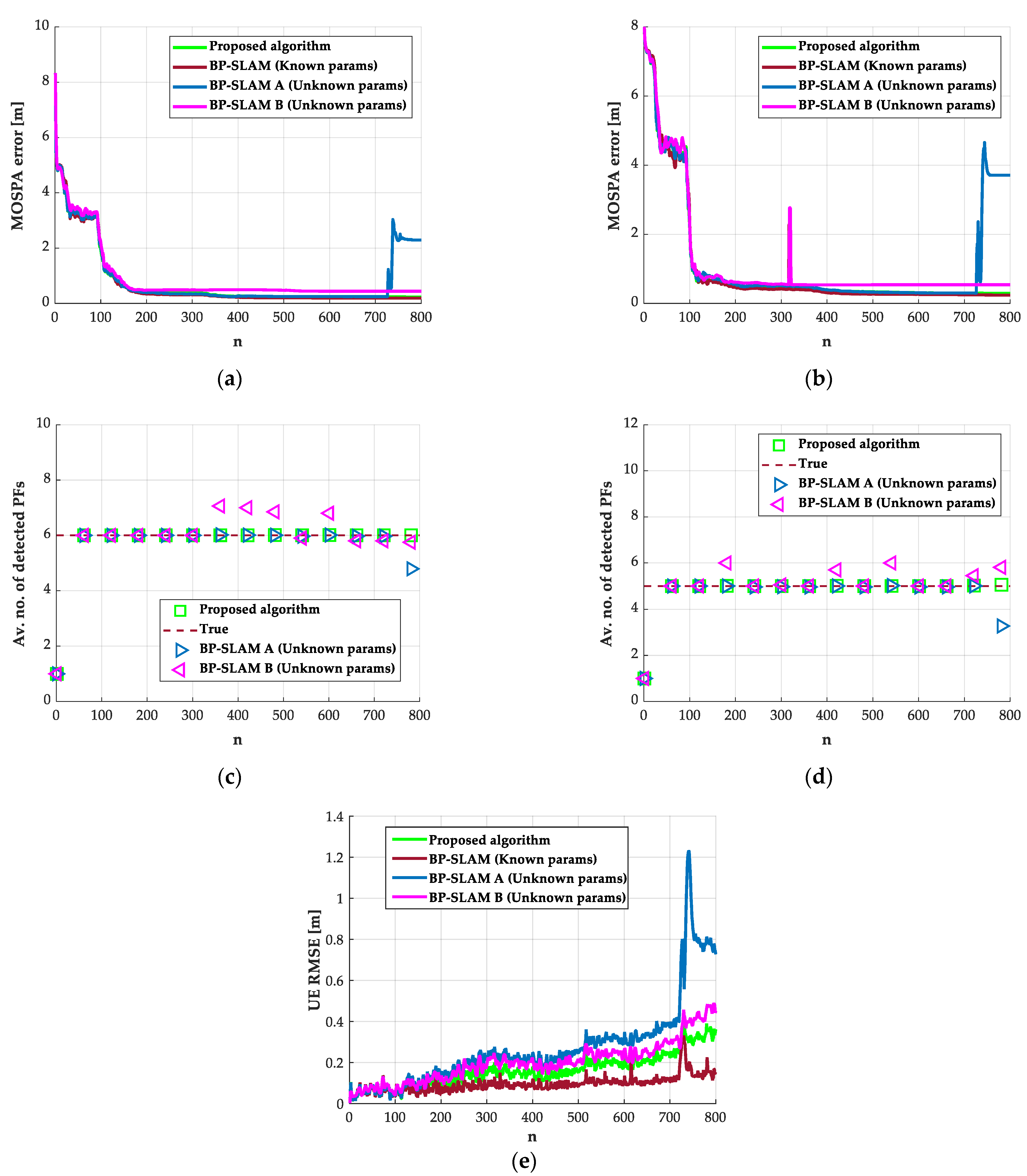
Figure 3 shows the performance of the proposed algorithm in the first scenario, which is obtained based on the average of 100 simulation runs. Figure 3a,b depict the mean optimal subpattern assignment (MOSPA) [45] errors for PT1 and PT2 and their associated VTs, respectively. The MOSPA error is based on Euclidean distance with a cutoff parameter of 5 m and order 1. The MOSPA error combines the estimation errors of correctly detected PFs and incorrectly detected PFs, which is often used as the standard to evaluate the mapping accuracy of multipath-assisted SLAM algorithms. In Figure 3a, period $n\in [0,720]$, the MOSPA error of BP-SLAM B for PT1 and its associated VTs is always higher than the other three algorithms. Then, when the UE process noise variance suddenly changes, i.e., $n\in [720,730]$, the MOSPA error of BP-SLAM A rises sharply with a maximum of more than 3 m. However, the MOSPA error of the proposed algorithm is always smaller than that of BP-SLAM A and BP-SLAM B in this period. This relationship still exists even after the UE returns to the normal motion state, i.e., $n\in [730,800]$. The MOSPA error for PT2 and its associated VTs shown in Figure 3b also have similar performance. Figure 3c,d describe the average number of detected PFs associated with PT1 and PT2, respectively. From these two figures, we can see that the average number of detected PFs for the proposed algorithm is always close to the actual number of features in the environment, namely, $L_n^{(1)}=6$ and $L_n^{(2)}=5$. However, the average number of detected PFs for BP-SLAM A deviates from the truth after 720 s, i.e., the UE process noise variance changes suddenly. The average number of detected PFs for BP-SLAM B deviates from the truth even when the UE process noise remains unchanged, i.e., $n\in [0,720]$. Figure 3e depicts the root mean square errors (RMSEs) of the UE position for the four algorithms. Figure 3e shows that in period $n\in [720,730]$, the UE position RMSE for BP-SLAM A rise sharply with a maximum of more than 1.2 m, while the UE position RMSE of the proposed algorithm is always less than 0.4 m in this period, which is close to the ideal BP-SLAM algorithm with known parameters. Although the UE position RMSE for BP-SLAM B has no sharp rise in this period, it is higher than that of the proposed algorithm all the time.

Table 2. Error statistics of different algorithms in the first scenario.

Algorithm	UE RMSE	MOSPA	No. of PFs
BP-SLAM A	0.2891 m	1.1143 m	0.1090
BP-SLAM B	0.1984 m	1.0442 m	0.2564
Proposed algorithm	0.1605 m	0.8759 m	0.0005
BP-SLAM (known params)	0.0949 m	0.7739 m	0 (True)

summarizes the error statistics of different algorithms in the first scenario within 800 s, including the average UE position RMSE, the average MOSPA error and the average error for the estimated number of detected PFs. The latter two errors are based on the average of PT1 and PT2 statistics. From Table 2, we can see that the statistical error of the proposed algorithm is significantly smaller than that of BP-SLAM A and BP-SLAM B, and close to the ideal BP-SLAM algorithm with known parameters. Therefore, Figure 3 and Table 2 both illustrate that the proposed algorithm is robust to the uncertainty of the process noise.

5.3. Second Scenario: Unknown Clutter Intensity Only

In the second scenario, we assume that only the clutter intensity parameter is unknown, which means that the UE does not have a sudden change in the dynamic model, with the process noise variance keeping ${\sigma }_p^2={0.01}^2$ during the movement. Therefore, it is unnecessary to consider the uncertainty of process noise in this scenario. The simulation time is also 800 s. Clutter is generated by a Poisson distribution with mean number ${\lambda }_{\mathrm{CL},n}^{(j)}=6$, and the spatial PDF of clutter is uniform in the ROI, i.e., $f_{\mathrm{CL}}(z_{m,n}^{(j)})=1/D$, where D is the area of the ROI. Thus, the clutter intensity can be expressed as $6/D$. We also compare the proposed algorithm with the conventional BP-SLAM algorithm with unknown parameters and the ideal BP-SLAM algorithm with known parameters in this scenario. Similar to the first scenario, we consider two parameter settings in the conventional BP-SLAM algorithm labeled BP-SLAM A and BP-SLAM B. They have no prior information on the true clutter intensity and just set this parameter by experience. BP-SLAM A and BP-SLAM B initialize the clutter intensity to $0.1/D$ and $12/D$, respectively. The ideal BP-SLAM algorithm with known parameters can obtain the prior information of the true clutter intensity in advance, which can also be used as the benchmark to evaluate the performance of our proposed algorithm in this scenario.

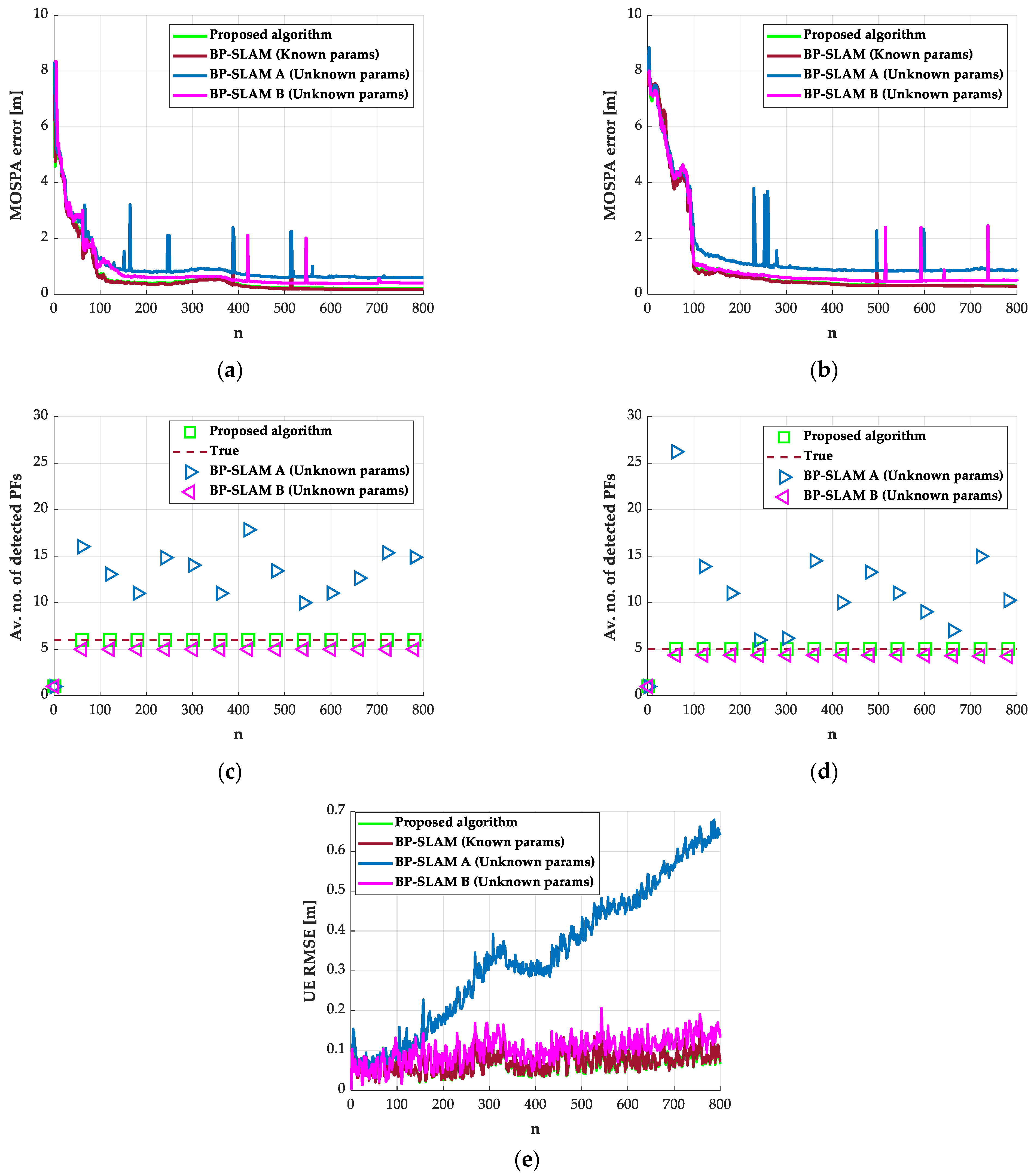
Figure 4 illustrates the simulation results of the proposed algorithm in the second scenario, which are also obtained based on the average of 100 simulation runs. Figure 4a,b show the MOSPA errors for PT1 and PT2 and their associated VTs, respectively. From Figure 4a, we see that the MOSPA errors of the four algorithms for PT1 all have a decreasing trend and finally reach steady states. The MOSPA errors for PT1 and the associated VTs of BP-SLAM A and BP-SLAM B converge at approximately 0.6 m and 0.4 m, respectively, while the performance of the proposed algorithm is better, converging near 0.2 m, which is close to the result of the BP-SLAM algorithm with known parameters. The results in Figure 4b are similar to those of Figure 4a. When the MOSPA error of the four algorithms becomes steady, the MOSPA error of the proposed algorithm is significantly smaller than that of BP-SLAM A and BP-SLAM B. Figure 4c,d describe the average number of detected PFs associated with PT1 and PT2 every 60 s, respectively. These two figures show that the average numbers of detected PFs by the proposed algorithm converge to the true values within 60 s, while the numbers of detected PFs by BP-SLAM A are always in a disordered state. Meanwhile, although the results for BP-SLAM B are convergent, they converge to the wrong number. Figure 4e depicts the UE position RMSEs for the four algorithms. Figure 4e shows that the position accuracy of the proposed algorithm is significantly better than that of BP-SLAM A and BP-SLAM B. During the simulation run time of 800 s, the RMSE of the proposed algorithm is always lower than 0.15 m, which is close to the performance of the BP-SLAM algorithm with known parameters. However, the UE position RMSE of BP-SLAM A increases rapidly in 800 s, and the maximum is more than 0.65 m. Although the performance of BP-SLAM B is relatively good, its position accuracy is lower than that of the proposed algorithm all the time.

Table 3. Error statistics of different algorithms in the second scenario.

Algorithm	UE RMSE	MOSPA	No. of PFs
BP-SLAM A	0.3768 m	1.2199 m	8.0151
BP-SLAM B	0.1083 m	1.0006 m	0.8329
Proposed algorithm	0.0741 m	0.7659 m	0.0678
BP-SLAM (known params)	0.0714 m	0.7376 m	0 (True)

summarizes the error statistics of different algorithms in the second scenario within 800 s. The MOSPA error and the error for the estimated number of detected PFs are also based on the average of PT1 and PT2 statistics. It can be seen from Table 3 that the statistical error of the proposed algorithm is significantly smaller than that of BP-SLAM A and BP-SLAM B, and close to the ideal BP-SLAM algorithm with known parameters. Therefore, Figure 4 and Table 3 both verify that the proposed algorithm is robust to the uncertainty of the clutter intensity.

5.4. Third Scenario: Unknown Process Noise and Clutter Intensity

In the third scenario, the uncertainty of the process noise and the clutter intensity are considered together, and the simulation time is 800 s. The variation in the UE process noise variance is the same as that in the first scenario. Most of the time, the UE process noise variance is ${\sigma }_{p_1}^2={0.01}^2$, but when $n\in [720,730]$, due to the sudden acceleration, the UE process noise variance changes to ${\sigma }_{p_2}^2={0.1}^2$. The BP-SLAM algorithm with unknown parameters considers that the UE process noise variance is fixed to ${\sigma }_p^2={\sigma }_{p_1}^2={0.01}^2$, while our proposed algorithm can adaptively switch between the two dynamic models with the transition matrix of the process noise variance the same as that in the first scenario. The generation mechanism of clutter is consistent with the second scenario. The true clutter intensity is $4/D$, but the proposed algorithm and the BP-SLAM algorithm with unknown parameters do not have this prior information. We also consider two parameter settings in the conventional BP-SLAM algorithm with unknown parameters in this scenario, labeled BP-SLAM A and BP-SLAM B. In BP-SLAM A, the UE process noise variance is fixed to ${\sigma }_p^2={\sigma }_{p_1}^2={0.01}^2$ and the clutter intensity is initialized to $0.1/D$ by experience. In BP-SLAM B, these two parameters are set to ${\sigma }_p^2={\sigma }_{p_2}^2={0.1}^2$ and $8/D$, respectively. In the third scenario, the BP-SLAM algorithm with known parameters can obtain the prior parameters of the process noise and the clutter intensity at each time in advance, which can still be used as the benchmark to evaluate the performance of the proposed algorithm.

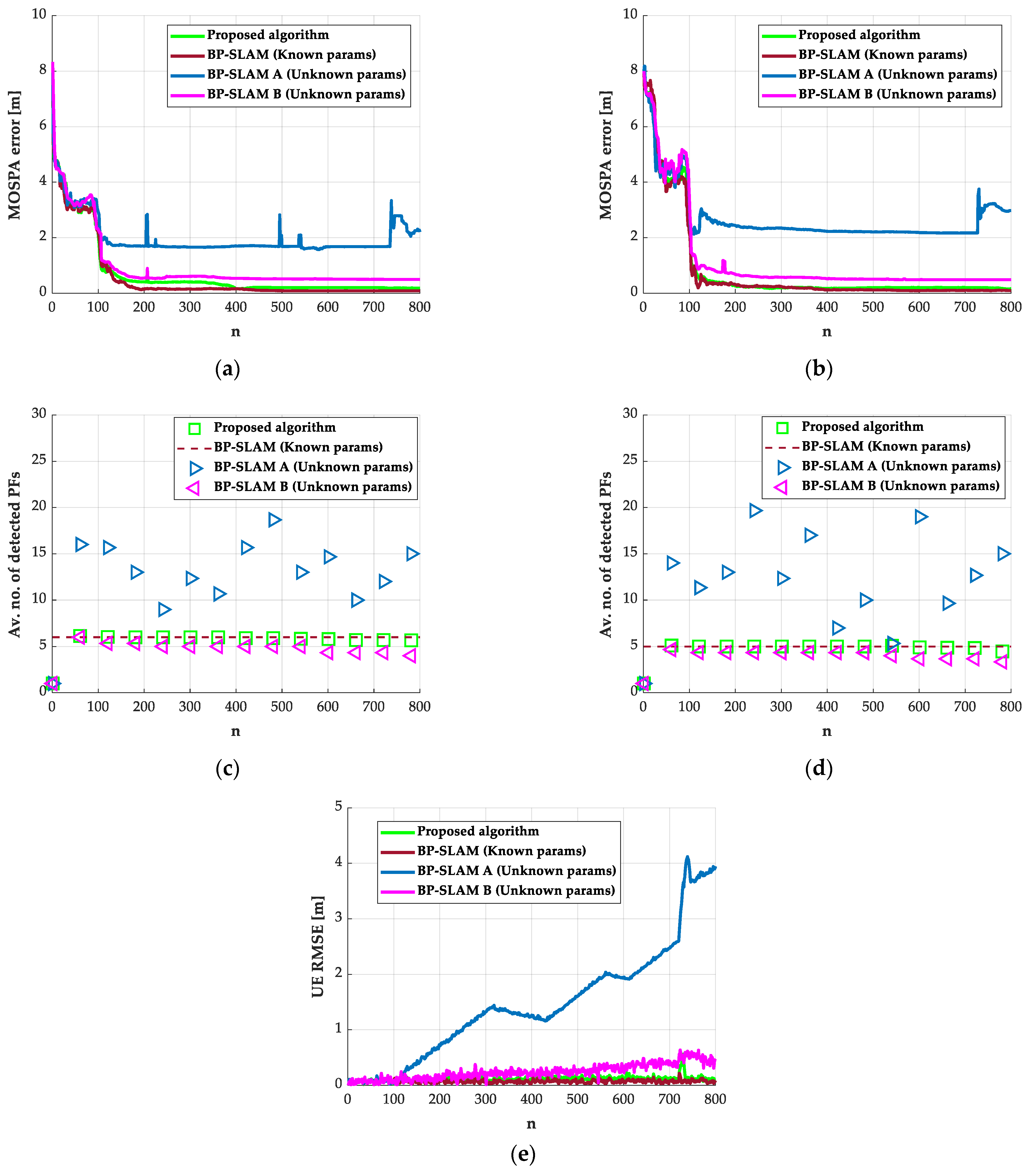
Figure 5 depicts the performance of the proposed algorithm in the third scenario, which is also obtained based on the average of 100 simulation runs. Figure 5a,b describe the MOSPA errors for PT1 and PT2 and their associated VTs, respectively. Figure 5a shows that the MOSPA errors of the four algorithms all reach steady states within approximately 150 s, and BP-SLAM A and BP-SLAM B are stable at approximately 1.8 m and 0.5 m, respectively. However, the performance of the proposed algorithm and the BP-SLAM algorithm with known parameters is obviously better with both below 0.3 m. In particular, the MOSPA error of BP-SLAM A rises sharply during the sudden change of the UE process noise variance, i.e., $n\in [720,730]$, and the maximum arrives near 3.2 m. The MOSPA errors of the proposed algorithm and the BP-SLAM algorithm with known parameters do not change significantly in this period. The MOSPA error for PT2 and the associated VTs described in Figure 5b has a similar performance to that in Figure 5a, i.e., regardless of whether the UE process noise changes, the performance of the proposed algorithm is better than that of BP-SLAM A and BP-SLAM B. Figure 5c,d show the average number of detected PFs associated with PT1 and PT2 every 60 s, respectively. These two figures show that the average numbers of detected PFs by the proposed algorithm are always near the true value, while the results of BP-SLAM A are not convergent. Although the results for BP-SLAM B are convergent, they converge on the wrong number. Therefore, in the third scenario, the estimation performance of the proposed algorithm for the average number of detected PFs is obviously better than that of BP-SLAM A and BP-SLAM B. Figure 5e describes the UE position RMSEs for the four algorithms in the third scenario. The time average RMSE of the proposed algorithm is 0.11 m within 800 s, while that of BP-SLAM A and BP-SLAM B are 1.46 m and 0.25 m, respectively. In particular, the time average RMSE of the proposed algorithm is 0.37 m when the UE process noise variance changes suddenly, i.e., $n\in [720,730]$, while BP-SLAM A and BP-SLAM B are 3.18 m and 0.55 m in this period. For the BP-SLAM algorithm with known parameters, the time average RMSE of the UE position is 0.07 m during 800 s and 0.11 m when $n\in [720,730]$. Based on the above data, the UE position accuracy of the proposed algorithm is significantly better than that of the BP-SLAM algorithm with unknown parameters and close to that of the BP-SLAM algorithm with known parameters.

Table 4. Error statistics of different algorithms in the third scenario.

Algorithm	UE RMSE	MOSPA	No. of PFs
BP-SLAM A	1.4636 m	2.2396 m	8.4696
BP-SLAM B	0.2452 m	1.0713 m	0.8099
Proposed algorithm	0.1121 m	0.7659 m	0.0628
BP-SLAM (known params)	0.0699 m	0.6738 m	0 (True)

summarizes the error statistics of different algorithms in the third scenario within 800 s. The MOSPA error and the error for the estimated number of detected PFs are also based on the average of PT1 and PT2 statistics. From Table 4, we can see that the statistical error of the proposed algorithm is significantly smaller than that of BP-SLAM A and BP-SLAM B, and close to the ideal BP-SLAM algorithm with known parameters. Therefore, Figure 5 and Table 4 show that the proposed algorithm is robust to both the clutter intensity and the process noise uncertainty.

5.5. Calculation Complexity Analysis

The computational complexity of the conventional BP-SLAM algorithm is proportional to $\mathcal{O}(N_{\mathrm{par}})$, where $N_{\mathrm{par}}$ is the number of particles [25]. The proposed algorithm adds the evolutions of the process noise variance and the clutter intensity to the Bayesian model compared with the conventional BP-SLAM algorithm; hence, its computational complexity is proportional to $\mathcal{O}(N_{\mathrm{par}}+N_b^2+N_g^2)$ [33], where $N_b$ and $N_g$ denote the number of process noise variances and clutter intensity, respectively. Considering that $N_b$ and $N_g$ are generally small compared to the number of particles $N_{\mathrm{par}}$, and therefore our proposed algorithm has nearly the same computational complexity as the conventional BP-SLAM algorithm. The average CPU run time consumed by each time step n in the third scenario is also used to compare the calculation complexity of different algorithms, where $N_{\mathrm{par}}=10000$, $N_b=2$ and $N_g=10$. The results of CPU run-time are based on 100 simulation runs and 800 time steps using a MATLAB implementation on an Intel Core i7-3632QM [email protected] GHz.

Table 5. Complexity comparison of different algorithms.

Algorithm	Complexity Order	CPU Run Time
BP-SLAM (unknown params)	$\mathcal{O}(N_{\mathrm{par}})$	0.0645 s
Proposed algorithm	$\mathcal{O}(N_{\mathrm{par}}+N_b^2+N_g^2)$	0.0761 s
BP-SLAM (known params)	$\mathcal{O}(N_{\mathrm{par}})$	0.0652 s

shows the complexity comparison of different algorithms in terms of both the complexity orders and the CPU run times. From Table 5, we can see that the proposed algorithm has almost the same calculation complexity as the conventional BP-SLAM algorithm with unknown parameters, but the performance of positioning and mapping accuracy is much better, close to the ideal BP-SLAM algorithm with known parameters. The reason is that the proposed algorithm considers the influence of the process noise and the clutter intensity uncertainty.

6. Conclusions

In multipath-assisted SLAM using radio signals, the estimation of the process noise and the clutter intensity is difficult in practice. Therefore, it is highly significant to study the multipath-assisted SLAM algorithm with the ability to adaptively estimate these unknown parameters. A robust multipath-assisted SLAM algorithm is proposed in this paper to solve the problem that the accuracy of the multipath-assisted SLAM algorithm decreases when the process noise and the clutter intensity are statistically uncertain. The proposed algorithm can still work with unknown time-varying parameters by continuously inferring an unknown parameter model, the states of the UE and environmental features. Specifically, we integrate the process noise variance and the clutter intensity into the factor graph representing the statistical structure of the SLAM problem and use the Markov chain model to describe the evolution of these unknown parameters. Finally, the BP message passing algorithm is performed to calculate the marginal posterior PDFs of each parameter to achieve the goal of simultaneous localization and mapping and adaptively learning the process noise variance and the clutter intensity.

The simulation results demonstrate that the proposed algorithm is superior to the conventional BP-SLAM algorithm in positioning and mapping accuracy with the uncertainty of the process noise and the clutter intensity. In particular, when the process noise and the clutter intensity are both unknown, the UE position time average RMSE at all times of the proposed algorithm is significantly less than that of the conventional BP-SLAM algorithm (0.11 m versus 1.46 m), and the performance in the MOSPA error and the average number of detected PFs is also obviously better than that of the conventional BP-SLAM algorithm (0.77 m versus 2.24 m and 0.06 versus 8.5, respectively), taking BP-SLAM A as an example. Therefore, the proposed algorithm can effectively restrain the impact of the process noise and the clutter intensity uncertainty on SLAM estimation accuracy and improve the robustness of a multipath-assisted SLAM system using radio signals.

We assume time synchronization between the transmitters and the UE in this paper. A promising direction for future research is the extension of our robust multipath-assisted SLAM algorithm to an unsynchronized sensor network.

References

1. Durrant-Whyte, H.; Bailey, T. Simultaneous localization and mapping: Part I. IEEE Robot. Autom. Mag. 2006, 13, 99–110. [Google Scholar] [CrossRef] [Green Version]
2. Bailey, T.; Durrant-Whyte, H. Simultaneous localization and mapping (SLAM): Part II. IEEE Robot. Autom. Mag. 2006, 13, 108–117. [Google Scholar] [CrossRef] [Green Version]
3. Lajoie, P.Y.; Ramtoula, B.; Chang, Y. DOOR-SLAM: Distributed, Online, and Outlier Resilient SLAM for Robotic Teams. IEEE Robot. Autom. Lett. 2020, 5, 1656–1663. [Google Scholar] [CrossRef] [Green Version]
4. Chiang, K.W.; Tsai, G.J.; Chu, H.J. Performance Enhancement of INS/GNSS/Refreshed-SLAM Integration for Acceptable Lane-Level Navigation Accuracy. IEEE Trans. Veh. Technol. 2020, 69, 2463–2476. [Google Scholar] [CrossRef]
5. Mendrzik, R.; Meyer, F.; Bauch, G. Enabling Situational Awareness in Millimeter Wave Massive MIMO Systems. IEEE J. Sel. Top. Signal Process. 2019, 13, 1196–1211. [Google Scholar] [CrossRef]
6. Chen, Z.; Zhu, G.; Wang, S. M3: Multipath Assisted Wi-Fi Localization with a Single Access Point. IEEE Trans. Mob. Comput. 2021, 20, 588–602. [Google Scholar] [CrossRef]
7. Ulmschneider, M.; Gentner, C.; Jost, T. Association of Transmitters in Multipath-Assisted Positioning. In Proceedings of the IEEE Global Communications Conference (GLOBECOM), Singapore, 4–8 December 2017. [Google Scholar]
8. Li, Z.; Tian, Z.; Wang, Z. Multipath-Assisted Indoor Localization Using a Single Receiver. IEEE Sens. J. 2021, 21, 692–705. [Google Scholar] [CrossRef]
9. Li, Z.; Tian, Z.; Wang, Z. Multipath-Assisted Indoor Localization: Turning Multipath Signal from Enemy to Friend. In Proceedings of the IEEE Global Communications Conference (GLOBECOM), Waikoloa, HI, USA, 9–13 December 2019. [Google Scholar]
10. Wielandt, S.; Strycker, L.D. Indoor Multipath Assisted Angle of Arrival Localization. Sensors 2017, 17, 2522. [Google Scholar] [CrossRef] [Green Version]
11. Witrisal, K.; Meissner, P.; Leitinger, E. High-accuracy localization for assisted living: 5G systems will turn multipath channels from foe to friend. IEEE Signal Process. Mag. 2016, 33, 59–70. [Google Scholar] [CrossRef]
12. Guidi, F.; Closas, P.; Dardari, D. Personal mobile radars with millimeter-wave massive arrays for indoor mapping. IEEE Trans. Mobile Comput. 2016, 15, 1471–1484. [Google Scholar] [CrossRef]
13. Guerra, A.; Guidi, F.; Dardari, D. Occupancy grid mapping for personal radar applications. In Proceedings of the IEEE Statistical Signal Processing Workshop (SSP), Freiburg, Germany, 10–13 June 2018. [Google Scholar]
14. Zhang, H.; Tan, S.Y. TOA based indoor localization and tracking via single-cluster PHD filtering. In Proceedings of the IEEE Global Communications Conference (GLOBECOM), Singapore, 4–8 December 2017. [Google Scholar]
15. Kim, H.; Granström, K.; Gao, L. 5G mmWave Cooperative Positioning and Mapping Using Multi-Model PHD Filter and Map Fusion. IEEE Trans. Wirel. Commun. 2020, 19, 3782–3795. [Google Scholar] [CrossRef] [Green Version]
16. Mendrzik, R.; Wymeersch, H.; Bauch, G. Joint Localization and Mapping through Millimeter Wave MIMO in 5G Systems. In Proceedings of the IEEE Global Communications Conference (GLOBECOM), Abu Dhabi, United Arab Emirates, 9–13 December 2018. [Google Scholar]
17. Leitinger, E.; Meissner, P.; Rudisser, C. Evaluation of position-related information in multipath components for indoor positioning. IEEE J. Sel. Areas Commun. 2015, 33, 2313–2328. [Google Scholar] [CrossRef] [Green Version]
18. Leitinger, E.; Meissner, P.; Witrisal, K. Simultaneous localization and mapping using multipath channel information. In Proceedings of the IEEE International Conference on Communication Workshop (ICCW), London, UK, 8–12 June 2015. [Google Scholar]
19. Gentner, C.; Ma, B.; Ulmschneider, M. Simultaneous localization and mapping in multipath environments. In Proceedings of the IEEE/ION Position, Location and Navigation Symposium (PLANS), Savannah, GA, USA, 11–14 April 2016. [Google Scholar]
20. Li, Z.; Tian, Z.; Wang, Z. WalkAround: Multipath-assisted Indoor Localization and Mapping Using a Single Receiver. In Proceedings of the IEEE International Conference on Communications (ICC), Dublin, Ireland, 7–11 June 2020. [Google Scholar]
21. Ulmschneider, M.; Gentner, C. Multipath assisted positioning for pedestrians using LTE signals. In Proceedings of the IEEE/ION Position, Location and Navigation Symposium (PLANS), Savannah, GA, USA, 11–14 April 2016. [Google Scholar]
22. Gentner, C.; Jost, T.; Wang, W. Multipath Assisted Positioning with Simultaneous Localization and Mapping. IEEE Trans. Wirel. Commun. 2016, 15, 6104–6117. [Google Scholar] [CrossRef] [Green Version]
23. Karásek, R.; Gentner, C. Stochastic Data Association for Multipath Assisted Positioning Using a Single Transmitter. IEEE Access 2020, 8, 46735–46752. [Google Scholar] [CrossRef]
24. Liu, Y.; Lian, B.; Zhou, T. Gaussian message pasing-based cooperative localization with node selection scheme in wireless networks. Signal Process. 2019, 156, 166–176. [Google Scholar] [CrossRef]
25. Leitinger, E.; Meyer, F.; Hlawatsch, F. A Belief Propagation Algorithm for Multipath-Based SLAM. IEEE Trans. Wirel. Commun. 2019, 18, 5613–5629. [Google Scholar] [CrossRef] [Green Version]
26. Leitinger, E.; Meyer, F.; Tufvesson, F. Factor Graph Based Simultaneous Localization and Mapping Using Multipath Channel Information. In Proceedings of the IEEE International Conference on Communications Workshops (ICC Workshops), Paris, France, 21–25 May 2017. [Google Scholar]
27. Leitinger, E.; Grebien, S.; Li, X. On the Use of Mpc Amplitude Information in Radio Signal Based SLAM. In Proceedings of the IEEE Statistical Signal Processing Workshop (SSP), Freiburg, Germany, 10–13 June 2018. [Google Scholar]
28. Leitinger, E.; Grebien, S.; Witrisal, K. Multipath-based SLAM Exploiting AoA and Amplitude Information. In Proceedings of the IEEE International Conference on Communications Workshops (ICC Workshops), Shanghai, China, 20–24 May 2019. [Google Scholar]
29. Bar-Shalom, Y.; Li, X.-R. Multitarget-Multisensor Tracking: Principles and Techniques; Yaakov Bar-Shalom: Storrs, CT, USA, 1995; pp. 1–4. [Google Scholar]
30. Mahler, R.P.S.; Vo, B.T.; Vo, B.N. CPHD Filtering with Unknown Clutter Rate and Detection Profile. IEEE Trans. Signal. Process. 2011, 59, 3497–3513. [Google Scholar] [CrossRef]
31. Vo, B.T.; Vo, B.N.; Hoseinnezhad, R. Robust multi-Bernoulli filtering. IEEE J. Sel. Top. Signal Process. 2013, 7, 399–409. [Google Scholar] [CrossRef]
32. Ristic, B.; Clark, D.; Vo, B.T.; Vo, B.N. Adaptive target birth intensity for PHD and CPHD filters. IEEE Trans. Aerosp. Electron. Syst. 2012, 48, 1656–1668. [Google Scholar] [CrossRef]
33. Soldi, G.; Meyer, F.; Braca, P.; Hlawatsch, F. Self-Tuning Algorithms for Multisensor-Multitarget Tracking Using Belief Propagation. IEEE Trans. Signal. Process. 2019, 67, 3922–3937. [Google Scholar] [CrossRef]
34. Kschischang, F.R.; Frey, B.J.; Loeliger, H.-A. Factor graphs and the sum-product algorithm. IEEE Trans. Inf. Theory 2001, 47, 498–519. [Google Scholar] [CrossRef] [Green Version]
35. Salmi, J.; Richter, A.; Koivunen, V. Detection and tracking of MIMO propagation path parameters using state-space approach. IEEE Trans. Signal. Process. 2009, 57, 1538–1550. [Google Scholar] [CrossRef] [Green Version]
36. Mahler, R.P.S. Statistical Multisource-Multitarget Information Fusion; Artech House: Norwood, MA, USA, 2007. [Google Scholar]
37. Jo, K.; Chu, K.; Sunwoo, M. Interacting Multiple Model Filter-Based Sensor Fusion of GPS With In-Vehicle Sensors for Real-Time Vehicle Positioning. IEEE Trans. Intell. Transp. 2012, 13, 329–343. [Google Scholar] [CrossRef]
38. Meyer, F.; Braca, P.; Willett, P.; Hlawatsch, F. A scalable algorithm for tracking an unknown number of targets using multiple sensors. IEEE Trans. Signal. Process. 2017, 65, 3478–3493. [Google Scholar] [CrossRef] [Green Version]
39. Wymeersch, H.; Seco-Granados, G. Adaptive Detection Probability for mmWave 5G SLAM. In Proceedings of the IEEE 2nd 6G Wireless Summit (6G SUMMIT), Levi, Finland, 17–20 March 2020. [Google Scholar]
40. Williams, J.L.; Lau, R. Approximate evaluation of marginal association probabilities with belief propagation. IEEE Trans. Aerosp. Electron. Syst. 2014, 50, 2942–2959. [Google Scholar] [CrossRef] [Green Version]
41. Meyer, F.; Kropfreiter, T.; Williams, J.L. Message passing algorithms for scalable multitarget tracking. Proc. IEEE 2018, 106, 221–259. [Google Scholar] [CrossRef]
42. Meyer, F.; Hlinka, O.; Wymeersch, H.; Hlawatsch, F. Distributed localization and tracking of mobile networks including noncooperative objects. IEEE Trans. Signal Inf. Process. Netw. 2016, 2, 57–71. [Google Scholar] [CrossRef] [Green Version]
43. Li, X.R.; Jilkov, V.P. Survey of maneuvering target tracking. part I. dynamic models. IEEE Trans. Aerosp. Electron. Syst. 2003, 39, 1333–1364. [Google Scholar] [CrossRef]
44. Horridge, P.; Maskell, S. Using a probabilistic hypothesis density filter to confirm tracks in a multi-target environment. In Proceedings of the Informatik Schafft Communities (INFORMATIK-11), Berlin, Germany, 4–7 July 2011. [Google Scholar]
45. Schuhmacher, D.; Vo, B.T.; Vo, B.N. A consistent metric for performance evaluation of multi-object filters. IEEE Trans. Signal Process. 2008, 56, 3447–3457. [Google Scholar] [CrossRef] [Green Version]
Figure 1. Example of an environment map.
Remotesensing 13 01625 g001
Figure 2. Factor graph representing the factorization of the joint posterior probability density function (PDF) in (30). All factor nodes, variable nodes and messages related to the user equipment (UE) augmented state are represented in red color, those related to legacy potential features (PF) states are represented in purple color, those related to new PF states are represented in blue color, and the section of the clutter intensity and the iterative data association (DA) are represented in orange color and green color, respectively. The abbreviations are defined as K K n ( j ) , M M n ( j ) , x x n , y _ k y _ k , n ( j ) , h k h k , n ( j ) , q m q m , n ( j ) , λ CL λ CL , n ( j ) , φ k , m φ ( h k , n ( j ) , q m , n ( j ) ) , c m c ( x n , a ¯ m , n ( j ) , e ¯ m , n ( j ) , q m , n ( j ) , λ CL , n ( j ) ; z n ( j ) ) , b k b ( x n , a _ k , n ( j ) , e _ k , n ( j ) , h k , n ( j ) , λ CL , n ( j ) ; z n ( j ) ) , f f ( x n | x n 1 ) , f k f ( y _ k , n ( j ) | y k , n 1 ( j ) ) , p p ( λ CL , n ( j ) | λ CL , n 1 ( j ) ) , α α ( x n ) , α k α k ( a _ k , n ( j ) , e _ k , n ( j ) ) , f f ( x n 1 ) , f f ( x n ) , f _ k f _ ( a k , n 1 ( j ) , e k , n 1 ( j ) ) , f _ k f _ ( a _ k , n ( j ) , e _ k , n ( j ) ) , f ¯ m f ¯ ( a ¯ m , n ( j ) , e ¯ m , n ( j ) ) , p p ( λ CL , n 1 ( j ) ) , p p ( λ CL , n ( j ) ) , β k β ( λ CL , n ( j ) ) , χ χ ( λ CL , n ( j ) ) , ε k ε ( h k , n ( j ) ) , ξ m ξ ( q m , n ( j ) ) , γ k γ ( h k , n ( j ) ) , ν m ν ( q m , n ( j ) ) , δ m , k δ m k ( t ) ( h k , n ( j ) ) , ς k , m ς k m ( t ) ( q m , n ( j ) ) , η k ( j ) η k ( j ) ( x n ) , η k η ( a _ k , n ( j ) , e _ k , n ( j ) ) , and μ m μ ( a ¯ m , n ( j ) , e ¯ m , n ( j ) ) .
Remotesensing 13 01625 g002
Figure 3. Results for the first scenario: (a) mean optimal subpattern assignment (MOSPA) error for physical transmitter (PT) 1 and the associated virtual transmitters (VTs); (b) MOSPA error for PT2 and the associated VTs; (c) average number of detected PFs associated with PT1 every 60 s; (d) average number of detected PFs associated with PT2 every 60 s; and (e) user equipment (UE) position root mean square errors (RMSEs).
Remotesensing 13 01625 g003
Figure 4. Results for the second scenario: (a) MOSPA error for PT1 and the associated VTs; (b) MOSPA error for PT2 and the associated VTs; (c) average number of detected PFs associated with PT1 every 60 s; (d) average number of detected PFs associated with PT2 every 60 s; and (e) UE position RMSE.
Remotesensing 13 01625 g004
Figure 5. Results for the third scenario: (a) MOSPA error for PT1 and the associated VTs; (b) MOSPA error for PT2 and the associated VTs; (c) average number of detected PFs associated with PT1 every 60 s; (d) average number of detected PFs associated with PT2 every 60 s; and (e) UE position RMSE.
Remotesensing 13 01625 g005