Abstract
Deep learning models have strong abilities in learning features and they have been successfully applied in hyperspectral images (HSIs). However, the training of most deep learning models requires labeled samples and the collection of labeled samples are labor-consuming in HSI. In addition, single-level features from a single layer are usually considered, which may result in the loss of some important information. Using multiple networks to obtain multi-level features is a solution, but at the cost of longer training time and computational complexity. To solve these problems, a novel unsupervised multi-level feature extraction framework that is based on a three dimensional convolutional autoencoder (3D-CAE) is proposed in this paper. The designed 3D-CAE is stacked by fully 3D convolutional layers and 3D deconvolutional layers, which allows for the spectral-spatial information of targets to be mined simultaneously. Besides, the 3D-CAE can be trained in an unsupervised way without involving labeled samples. Moreover, the multi-level features are directly obtained from the encoded layers with different scales and resolutions, which is more efficient than using multiple networks to get them. The effectiveness of the proposed multi-level features is verified on two hyperspectral data sets. The results demonstrate that the proposed method has great promise in unsupervised feature learning and can help us to further improve the hyperspectral classification when compared with single-level features.
1. Introduction
Hyperspectral images (HSIs) are collected by hyperspectral imaging sensors from the visible to the near-infrared wavelength ranges, which contains hundreds of spectral bands. HSIs are three-dimensional (3D) data providing not only spatial information, but also spectral information. Benefiting from these characteristics, HSIs have been applied in many fields and the ability to differentiate the interesting targets is improved when compared with two-dimensional (2D) images [1,2,3]. Feature extraction is a significant step in realizing these applications. Traditional manual feature extraction methods are time-consuming and susceptible to external influences. In recent years, deep learning models have shown great potential in mining data information automatically and flexibly, which has been successfully applied in image processing [4,5,6,7], natural language processing [8,9,10,11], and other fields [12,13,14,15]. Among the deep learning models, convolutional neural networks (CNNs) have attracted widespread attention due to their unique network structure and superior performance. Multi-dimensional data can be directly used as the input of CNN. Some models based on three-dimensional convolutional neural network (3D-CNN) have been designed to fully exploit the spectral-spatial features of HSIs and obtain good performance [16,17,18]. However, the training procedure of CNN is supervised and the network is optimized by minimizing the output and label error, which means that a large number of labeled samples are required to guarantee the network performance. Worse, the labeled samples are limited in HSIs and the collection is costly [19,20].
Fortunately, there are still some models that do not require labels for training. Generative adversarial networks (GANs) are trained in an adversarial way [21,22]. GAN mainly consist of two parts: a discriminator and generator. Generator captures the probability distributions of real data by mapping noise to synthetic data. Discriminator decides whether the input data are real or synthetic. The generator tries to generate images to fool the discriminator and the discriminator strives to distinguish the generated images. Through this adversarial training, the network is continuously optimized without labeled samples. Some of the unsupervised feature learning methods based on GAN have been developed in [23,24,25]. In addition, the autoencoder (AE) learns a representation for input data through an encoder and then decodes the representation to reconstruct data [26,27]. The AE can be optimized by minimizing the error between the reconstructed data and the input data, and no labels are involved, which is a typical unsupervised model. Because of these characteristics of AE, some unsupervised feature extraction methods that are based on AE have been introduced in HSIs and achieved some results [28,29,30,31].
However, when models are developed for unsupervised feature extraction, features from the single layer are usually considered, which will lose some useful information [32]. The image pyramid framework, which uses different-scale images to independently train multiple networks to obtain multi-level features is one of the solution [33], but training multiple networks increases the time and computational cost, which is unsatisfactory. The encoder of a AE and the discriminator of a GAN are hierarchical structures from bottom to top, and they are like feature pyramids. The bottom layer mainly corresponds to information, such as edges, texture, and contours, and the top layer mainly corresponds to semantic information. When considering the construction and training of AE is easier than GAN, an unsupervised multi-level feature extraction method based on a three dimensional convolutional autoencoder (3D-CAE) is proposed in this paper. The designed 3D-CAE is composed of 3D convolutional layers and 3D deconvoluional layers, combining the advantages of CNN and AE. The 3D-CAE can not only fully mine the spectral-spatial information with 3D data as input, but it also does not require the participation of labeled samples in the training process. In addition, multi-level features are directly obtained from different encoded layers of the optimized encoder, which is more efficient when compared to training multiple networks. The full use of the detail information at the bottom layer and semantic information at the top layer can achieve complementary advantages and improve the classification results.
The remainder of this paper is organized, as follows. Section 2 provides some basic knowledge of convolution and deconvolution operations. Section 3 describes the details of proposed multi-level features based on 3D-CAE. Section 4 provides an analysis and comparison of experimental results. Section 5 concludes this paper.
2. Preliminaries
2.1. Convolution Operation
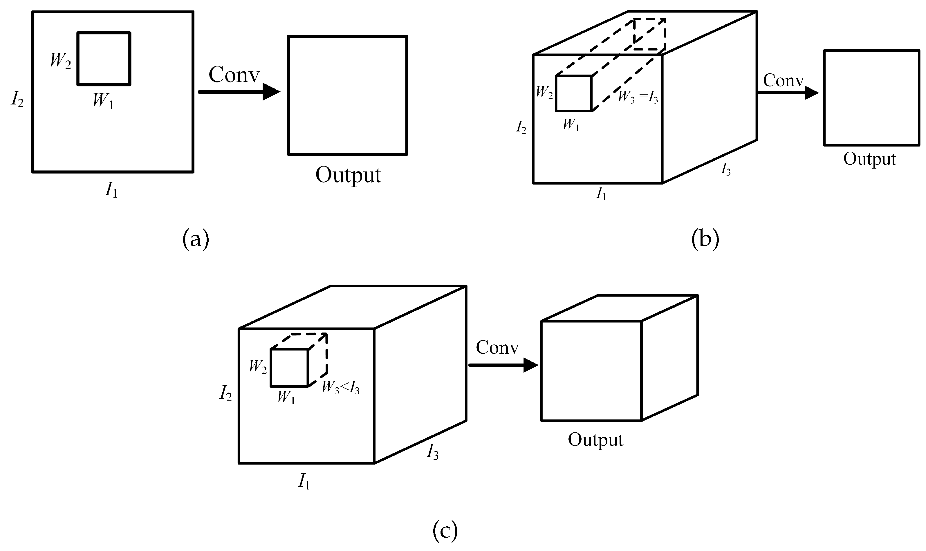
Convolution operations have been widely used in signal processing and image processing. They apply convolution kernels to an input image to produce feature maps, which shows great potential in feature extraction. There are three main ways of convolution operation [34]: 2D convolution for a single-channel, 2D convolution for multi-channel, and 3D convolution, as shown in Figure 1.
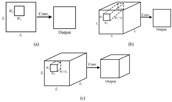
Figure 1.
Convolution operation: (a) 2D convolution for a single-channel, (b) 2D convolution for multi-channel, (c) 3D convolution.
It can be seen from Figure 1a that 2D convolution for a single-channel is performed on 2D input data, and a 2D output is obtained by sliding, which has great potential to retain the spatial information of the data. We can find, from Figure 1b,c, that both 2D convolution for multi-channel and 3D convolution can be performed on 3D data. However, since the depth of the convolution filter in 2D convolution for multi-channel is the same as the depth of the data, it can only move in two directions (width and height of the data) and obtain a 2D output. The 3D filter in 3D convolution can move in three directions (width, height, and depth of data) and each movement of the filter can obtain a value by element-wise multiplication and addition. The output of 3D convolution is a 3D data.
Taking 3D convolution as an example, when the input is I , the convolution kernel is W , and the stride is , its output is defined as:
where means the output at position , denotes the kernel value of position and b is the bias.
Each convolution kernel corresponds to an output (feature map), and different convolution kernels can extract different features.
2.2. Deconvolution Operation
Transposed convolution, which is also called deconvolution, is like the reverse process of convolution. Figure 2 shows an example of 2D convolution for a single-channel and its corresponding 2D deconvolution.
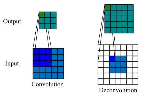
Figure 2.
2D convolution and 2D deconvolution.
It can be observed, from Figure 2, that, during the convolution process without padding, the output size is unusually less than the input size, while, in the deconvolution process, the output size is often larger. Because of this property of deconvolution, it is often used when generating or reconstructing images. Similar to the convolution mode, deconvolution operation also has three corresponding modes.
According to the characteristics of the target data, we can flexibly choose the convolution operation mode. For ordinary 2D data, 2D convolution for a single-channel is good for learning features and the computational complexity is relatively low. For multi-dimensional or high-dimensional data, the 3D convolution may have more potential in mining features.
3. Proposed Framework for Multi-Level Feature Extraction
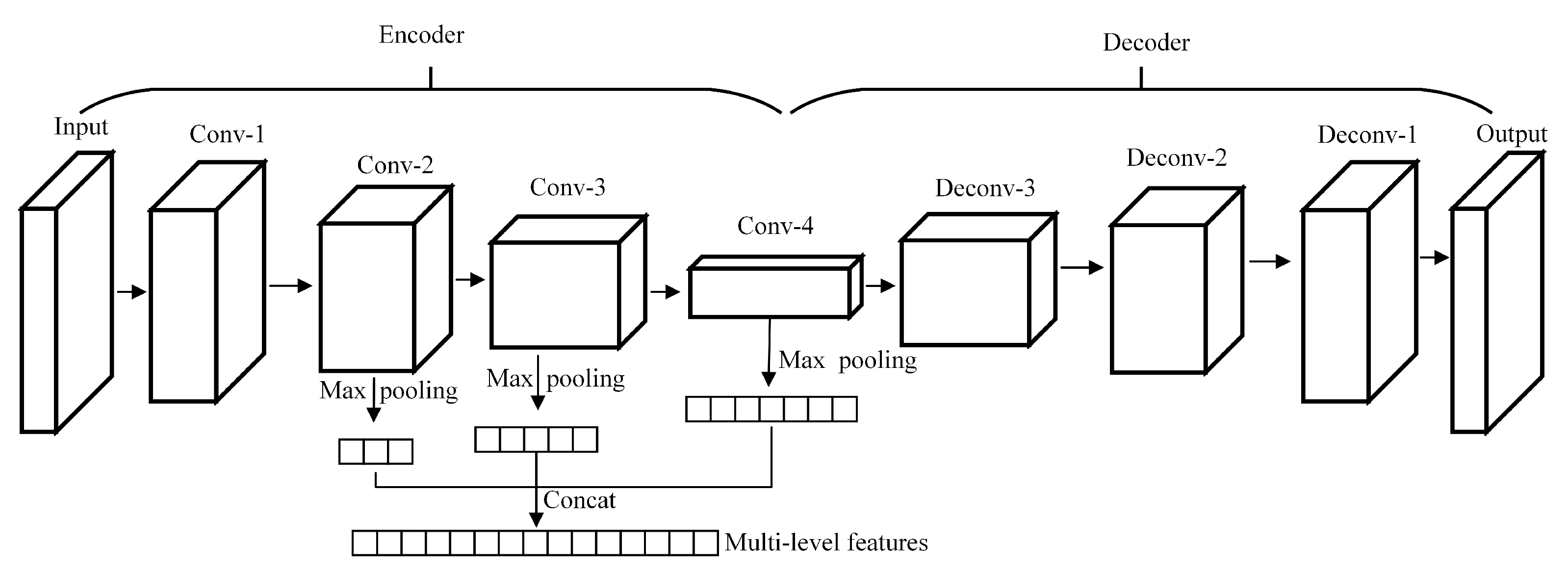
A traditional AE is usually composed of fully connected layers and it takes a one-dimensional (1D) vector as input, which destroys the original spatial structure of the data. This is because convolution-based operation has high flexibility in processing multi-dimensional data and has a strong ability in feature extraction. A 3D-CAE with convolutional layers instead of fully connected layers is designed in this paper, which makes the input form of the network more variable. HSIs are 3D tensor data containing hundreds of spectral bands, which can provide abundant spectral and spatial information. In order to better preserve the spatial and spectral characteristics of data, the designed 3D-CAE is established by fully 3D convolutional layers and 3D deconvolutional layers (see Figure 3), where Conv-n and Deconv-n mean the nth convolutional layer and the nth deconvolutional layer, respectively. For each pixel in HSIs, a 3D block centred on the current observed pixel is used as the input of 3D-CAE to learn its invariant characteristics.
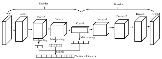
Figure 3.
The proposed framework for multi-level feature extraction.
The proposed framework for multi-level feature learning is mainly divided into three steps:
Firstly, a 3D-CAE is constructed. The 3D-CAE is designed as a symmetrical structure composed of 3D convolutional layers and deconvolutional layers, as shown in Figure 3. The size of feature map is gradually reduced, and the number of convolution kernels is gradually increased. The size of output is the same as the size of input.
Secondly, train and optimize the 3D-CAE network. The data are input into the 3D-CAE and encoded as a low-dimensional representation through the encoder. The decoder is responsible for recovering the original input data from the representation. The 3D-CAE is constantly adjusted by minimizing the error between the output () and input (), as described in Equation (2). When the network can reconstruct the input data well, we believe that the network has a strong ability to mine the useful information in the data.
Thirdly, obtain multi-level features from the optimized encoder. The hierarchical structure of the encoder from the bottom to top provides us with features of different levels and different scales. Max-pooling is introduced to reduce the feature dimension and increase feature invariance [35]. The filter size of max-pooling is set to equal to the size of the corresponding feature map. Through pooling operations, each layer can get a feature vector containing different information. The final features are concatenated by these feature vectors from multiple layers of encoder to make them contain more information and have high scale robustness. It is worth noting that the proposed multi-level features from a single network. When compared with training multiple networks to obtain multi-level features, the proposed method is more effective and saves training time. Our expectation is to make full use of the well-trained network to obtain as much information as possible, and then help to improve the subsequent classification accuracy.
4. Experiments
4.1. Data Set Description
In order to compare and study the performance of the proposed feature extraction method, experiments are performed on two real-world data sets: Pavia University (Figure 4a) and Indian Pines (Figure 4c). Pavia University data set is acquired by ROSIS sensor, which contains 103 spectral bands. There are 610 × 340 pixels covering nine categories. The Indian Pines data set collected by AVIRIS sensor consists of 145 × 145 pixels and 220 spectral bands after removing low-signal bands. This scene mainly contains agriculture and vegetation, and it is designated into sixteen classes. Figure 4b,d are the ground truth of the two data sets, respectively, and each color corresponds to a land-cover class of the current scene, where black represents the unlabeled area.
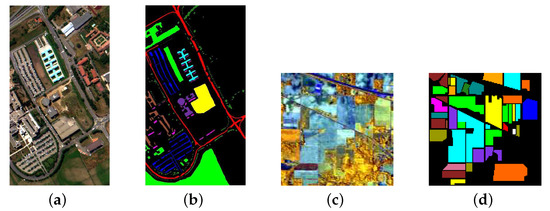
Figure 4.
Data sets: (a) Composite image of Pavia University, (b) Ground truth of Pavia University, (c) Composite image of Indian Pines, and (d) Ground truth of Indian Pines.
4.2. Network Construction
The bands of the two data sets are reduced to 10 by principal component analysis (PCA) in order to reduce the amount of calculation and improve the efficiency of network training [36,37]. For each pixel in HSIs, a 3D block with a size of centered on the observed pixel is selected as the input to construct the network, where represents the spatial neighborhood window around the observed pixel and L means the retained principal components. The network structure is given in Table 1 while taking as an example. When considering that the established 3D-CAE is symmetrical, only the parameter settings of the encoder are listed.

Table 1.
Network structures of encoder in proposed three dimensional convolutional autoencoder (3D-CAE).
In Table 1, Conv-n represents the nth convolutional layer and kernel of means that there are convolution kernels with kernel size being in the current layer. Besides, the stride is set to during the convolution operation. Rectified linear unit (ReLU) is mainly used as an activation function to introduce nonlinear mapping into the network, except for the last deconvolution layer with sigmoid. Adam is selected as the optimizer to update the weights [38].
4.3. Comparison and Analysis of Experimental Results
Classification results based on different features (single-level features and multi-level features) are considered for comparison to better evaluate the effectiveness of the multi-level features. The better the classification result, the better the corresponding features. In the experiment, support vector machine (SVM) is selected as the classifier. Overall accuracy (OA), average accuracy (AA), and kappa coefficient () are introduced to evaluate the classification results. If there are N classes in a data set and the number of samples in the n-th class is . Thus, the total number of samples is (). denotes the number of test samples that actually belong to the n-th class, and are also classified into n-th class. The OA, AA, and values can be defined as:
For each class in data sets, approximately 10% is used to train the classifier and the rest is used for testing. The details of the land-cover classes and the number of samples in Pavia University and Indian Pines are listed in Table 2 and Table 3, respectively, where each color corresponds to a land-cover class.

Table 2.
Land-cover classes and color coding in Pavia University.

Table 3.
Land-cover classes and color coding in Indian Pines.
At first, single-level features and multi-level features from three encoded layers are compared under the condition of input size being . When considering that the number of encoded layers used to form multi-level features may also affect the classification results, we will study the influence of this parameter on the results later. As shown in Figure 5, the feature map size in top three layers (third, fourth, and fifth) of encoder is , , and , respectively. Therefore, the filter size of max-pooling in the third and fourth layers is correspondingly set as and . The feature map size of the fifth layer is already , so we directly flatten the feature maps into a 1D vector. After max-pooling operation, three feature vectors are obtained with sizes of , , and . The three feature vectors are concatenated to obtain a final feature vector with the size being . These features are fed into the classifier, and the prediction results can be obtained, where Prediction I represents the predicted classification results based on the final multi-level features with a size of , Prediction II represents the results of single-level features from the fifth layer, Prediction III corresponds to the single-level features with a size of , and Prediction IV corresponds to the single-level features with a size of .
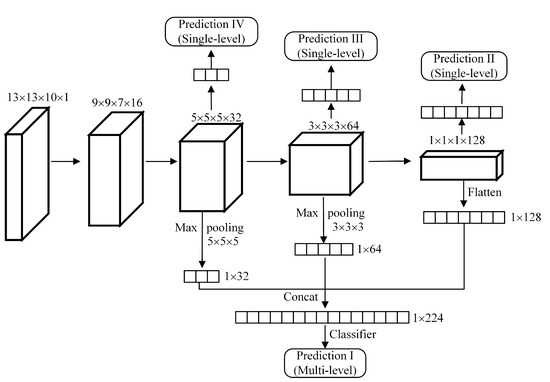
Figure 5.
Different features from the encoder of 3D-CAE for classification.
Table 4 and Table 5 list the classification results that are based on different features of Pavia University and Indian Pines.

Table 4.
The classification accuracy of Pavia University based on different features.

Table 5.
Classification accuracy of Indian Pines based on different features.
For the Pavia University data set, it can be observed from Table 4 that Prediction II based on features from top layer of encoder are better when compared with Prediction III and Prediction IV when only single-level features are considered. The classification accuracy of Class 2 (Meadows), Class 6 (Bare soil) and Class 7 (Bitumen) is less than 90% in Prediction III and Prediction IV, which is not satisfactory. Although the relevant results in Prediction II are improved, the classification accuracy of Class 6 (Bare soil) and Class 7 (Bitumen) is still not good. When multi-level features are used for classification, the classification accuracy of each category exceeds 90%. Moreover, the results of Prediction I are approximately 2% higher than Prediction II in OA, AA, and .
For Indian Pines data set, when single-level features are used for classification, it can be found from Table 5 that the performance of the single-level features (Prediction IV and Prediction III) from the third and fourth layers of encoder are not as good as that from top layer (the fifth layer) of encoder. Prediction II is the best among classification results based on single-level features, but the classification accuracy of Class 7 (Grass-pasture-mowed), Class 9 (Oats), Class 13 (Wheat) and Class 15 (Buildings-grass-trees) is less than 80%. When multi-level features are used for classification, the classification accuracy of these four targets are increased by 14%, 25%, 7%, and 7%, respectively. In addition, the highest OA, AA, and values are achieved when multi-level features are used. Prediction I outperforms any result based on single-level features, which proves that multi-level features allow us to obtain more useful information.
In general, it can be seen, from Table 4 and Table 5, that the proposed multi-level features obtain the highest OA, AA, and values for the two data sets and the classification accuracy of most land-cover classes is improved when compared to the results that were obtained by other features. However, the classification accuracy of some classes is always lower than other classes under different features, such as Class 7 (Bitumen) in Pavia University and Class 7 (Grass-pasture-mowed) and Class 13 (Wheat) in Indian Pines. From Table 2 and Table 3, we can see that the number of samples in these classes is relatively small. Besides, the within-class variation and inter-class similarity also reduce the classification accuracy. Because of the similarity of Class 1 (Asphalt) and Class 7 (Bitumen) in Pavia University, some pixels that belong to Class 7 are misclassified as Class 1 with more samples. Similarly, some pixels that belong to Class 13 (Wheat) are misclassified as Class 6 (Grass-trees) in Indian Pines. Therefore, the classification accuracy may be lower if the number of samples is small or there are similar classes in the current scene.
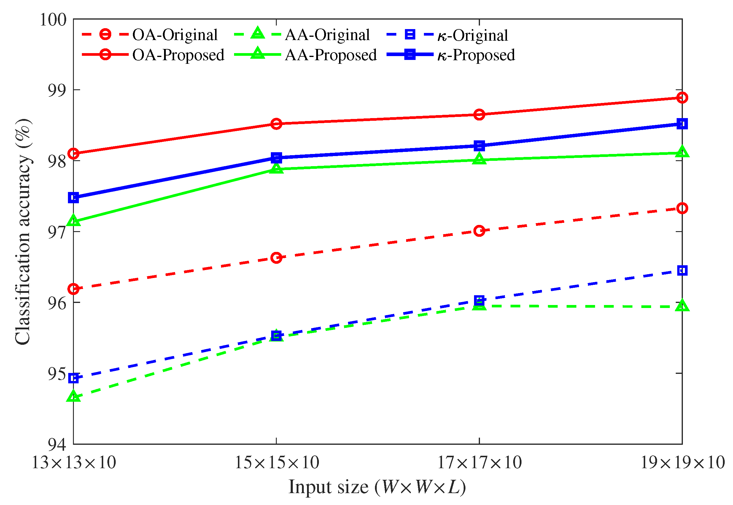
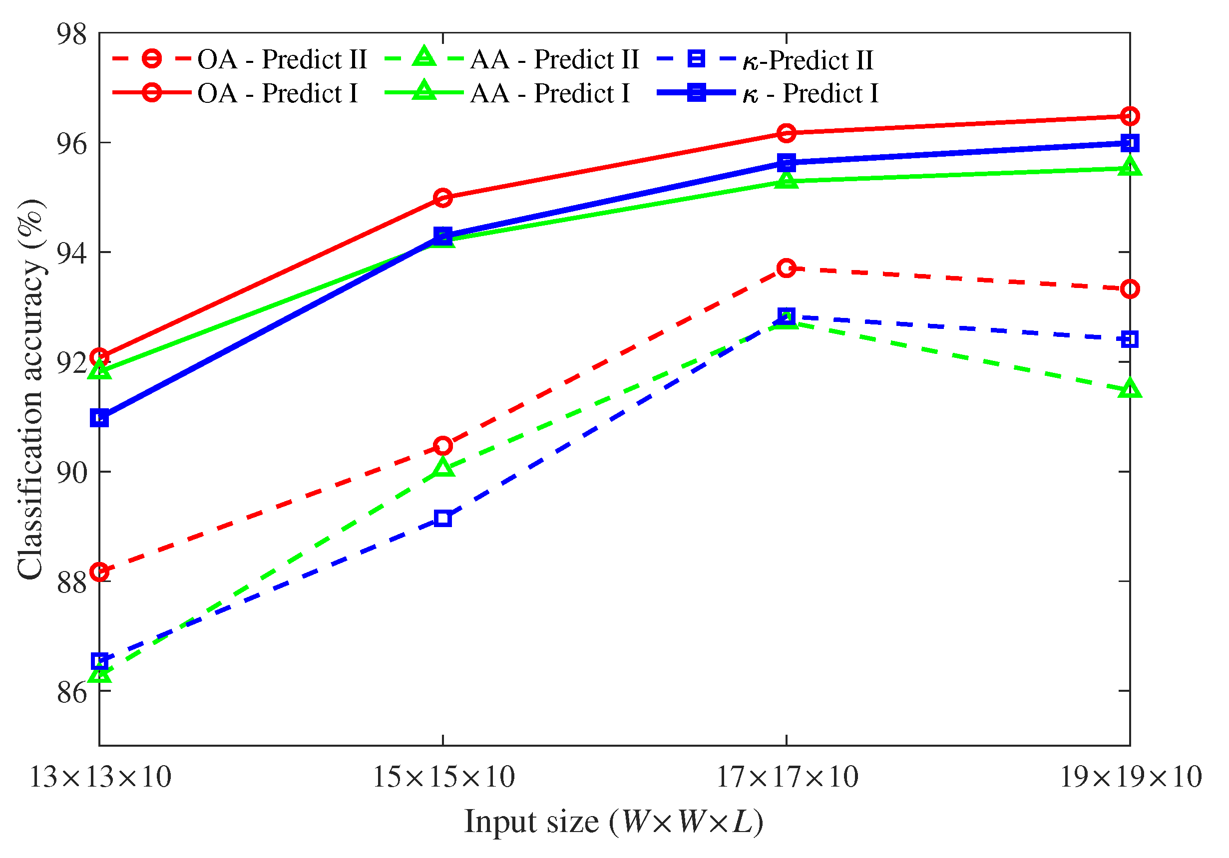
Both of the results shown in Table 4 and Table 5 are obtained under the condition that the input size is . When the input size changes from to , the classification accuracy based on single-level features from top encoded layer (Prediction II) and multi-level features (Prediction I) are compared. The comparison results of Pavia University and Indain Pines are depicted in Figure 6 and Figure 7, respectively.
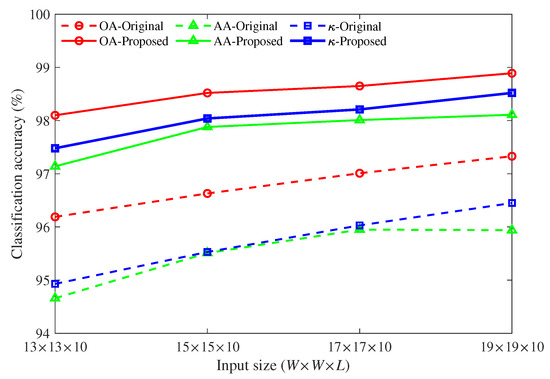
Figure 6.
Classification accuracy of Pavia University under different input sizes.
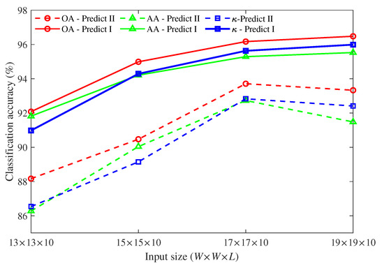
Figure 7.
The classification accuracy of Indian Pines under different input sizes.
For the Pavia University data set, we can find, from Figure 6, that when the input size increases from to , whether single-level features or multi-level features are used for classification, the OA, AA, and values gradually increase. But as the size increases, the amount of calculation and network training time will also increase. Moreover, the performance of multi-level features always outperforms single-level features. The OA, AA, and values increased by about 2% to 3% on average as compared with the results of single features.
For Indian Pines data set (Figure 7), when single-level features are used for classification, we find that the input size greatly affects the classification accuracy. The classification accuracy initially increases as the input size and it reaches a peak at , and then begins to decline. When multi-level features are used for classification, the classification accuracy is relatively stable except when the input size is . When the input size is fixed, the performance of multi-level features is much better than single-level features. When compared with the results of single-level features, the classification values improve about 2% to 5%. Even the peak value of a single-level features is about 2% lower than that of multi-level features.
In general, the results that are based on multi-level features are better than those of single-level features for both data sets, which proves that the multi-level features have more potential in hyperspectral classification.
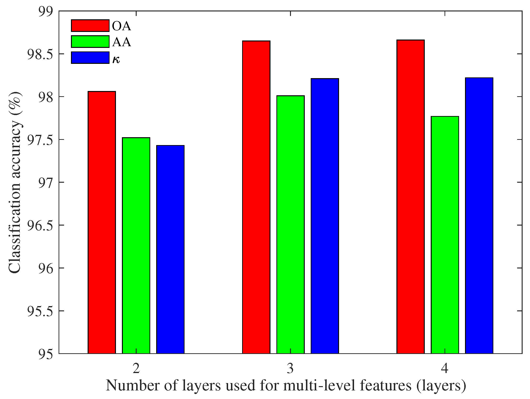
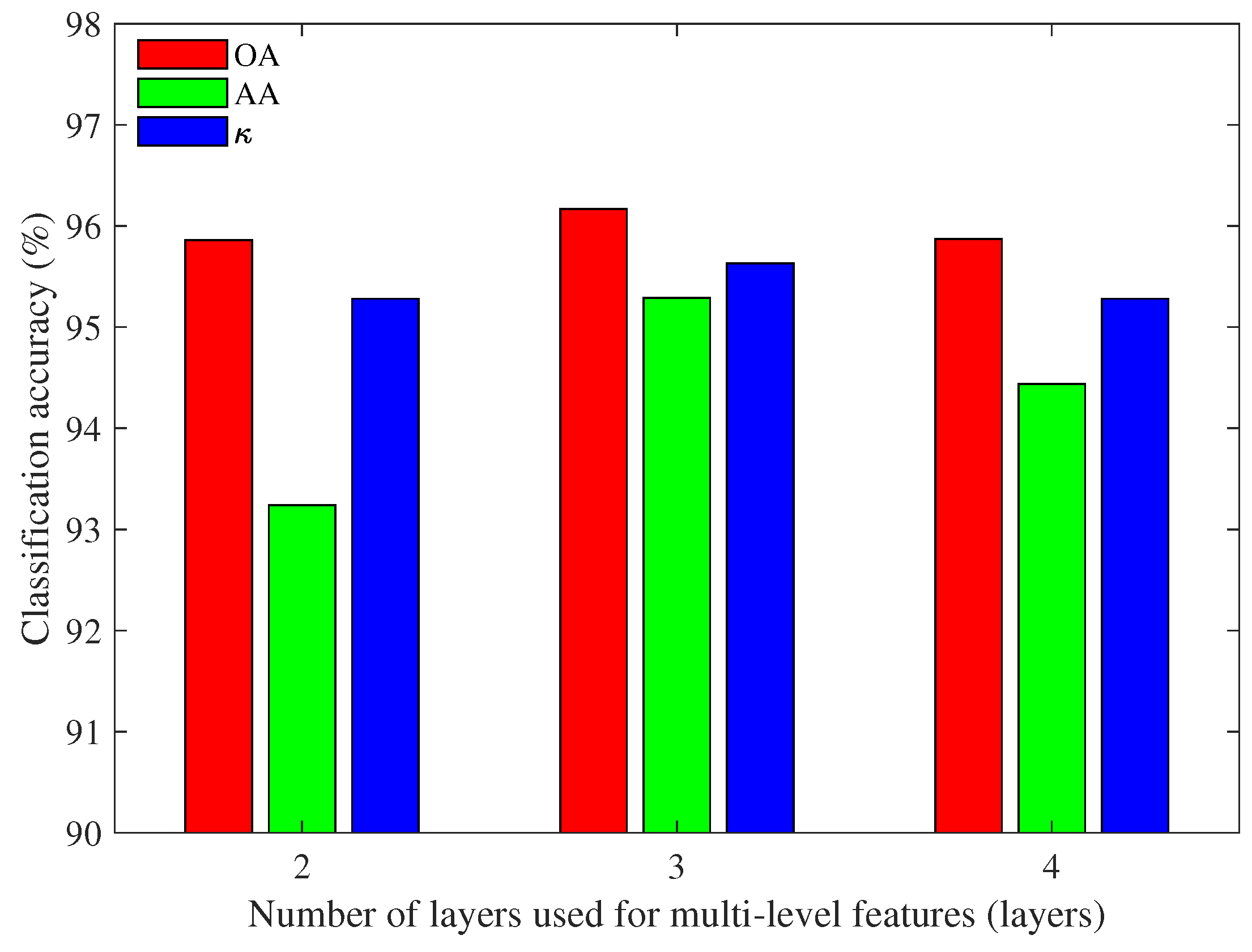
In the previous experiment, the multi-level features are obtained by concatenating the information of three encoded layers. In order to observe the impact of the number of encoded layers on the classification results, the multi-level features obtained from two, three, and four encoded layers are compared with input size being . The comparison results of Pavia University and Indian Pines data sets are shown in Figure 8 and Figure 9, respectively.
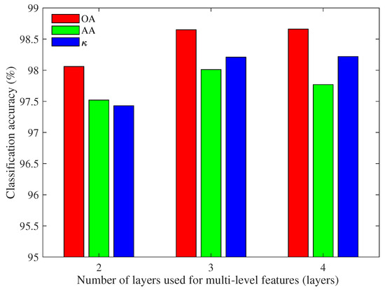
Figure 8.
Classification accuracy of Pavia University based on multi-level features with different numbers of encoded layers.
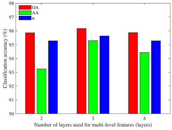
Figure 9.
Classification accuracy of Indian Pines based on multi-level features with different numbers of encoded layers.
It can be observed from Figure 8 that the performance of multi-level features obtained by using three and four encoded layers are better than that of two encoded layers. When considering that the results of three and four encoded layers are similar and the feature dimension obtained by three encoded layers is lower, three encoded layers used to concatenate features are more appropriate for Pavia University. Therefore, three is selected as the number of encoded layers for multi-level features in the subsequent experiments.
For the Indian Pines data set (Figure 9), the OA and values are slightly affected by the number of encoded layers. But the AA values based on two encoded layers and four encoded layer are relatively low. Therefore, three encoded layers are more suitable for obtaining multi-level features for Indian Pines.
Next, supervised feature extraction methods based on deep belief network (DBN), two dimensional convolutional neural network (2D-CNN), and unsupervised feature extraction method based on factor analysis (FA), stacked autoencoder (SAE) are considered for comparison to better evaluate the performance of the proposed method with the input size being and the number of encoded layers for multi-level features being three. DBN is composed of multiple layers of latent variables and it usually takes a 1D vector as input, which learns deep features via pretraining in a hierarchal manner [39,40,41]. 2D-CNN directly takes 2D data as input, which can better preserve the spatial structure of the target. FA is a linear statistical method that uses fewer numbers of factors to replace original data [42]. SAE is stacked by multiple AEs that can be used to learn a higher-level representation of input data [43,44]. The relevant results of Pavia University and Indian Pines under different methods are given in Table 6 and Table 7, where FE represents feature extraction.

Table 6.
Classification accuracy of Pavia University based on different feature extraction methods.

Table 7.
Classification accuracy of Indian Pines based on different feature extraction methods.
For the Pavia University data set, we can see from Table 6 that the OA, AA, and values of FA are the lowest, which reflects that deep learning models have more strong ability in feature extraction. When DBN and SAE are used for extracting features, the classification accuracy of Class 1 (Asphalt), 3 (Gravel) to 5 (Metal sheets) and 9 (Shadows) is relatively high. When 2D-CNN is introduced to obtain features, although the classification accuracy of Class 1 (Asphalt), 4 (Trees), and 9 (Shadows) is not as good as that of DBN and SAE, the accuracy of most other classes is improved, especially the OA value. This is because the inputs of DBN and SAE are one-dimensional (1D) vectors, while 2D-CNN can take 2D matrices as input, which can better retain the spatial information of the target. Among all of the deep models considered, the results based on 3D-CAE are more satisfactory. When compared with single-level features, multi-level features can help us to further improve the classification accuracy. Especially for Class 7 (Bitumen), the accuracy obtained by other feature extraction methods is less than 90%, but the introduction of multi-level features reaches 95%. Overall, the highest OA, AA, and values are obtained by the proposed multi-level features.
For Indian Pines data set, the classification results of FA are not good, and the classification accuracy of most classes is less than 90%. DBN and SAE help us to improve the classification accuracy to a certain extent, but it is still not satisfactory. The OA and values based on 2D-CNN and CAE-based model exceed 90%, which demonstrate that convolution-based operations are more flexible and have strong feature extraction capabilities. Besides, the OA, AA, and values that are based on multi-level features improved by about 3%, 1%, and 3% when compared with single-level features. Therefore, the proposed multi-level features can help us to further improve the classification.
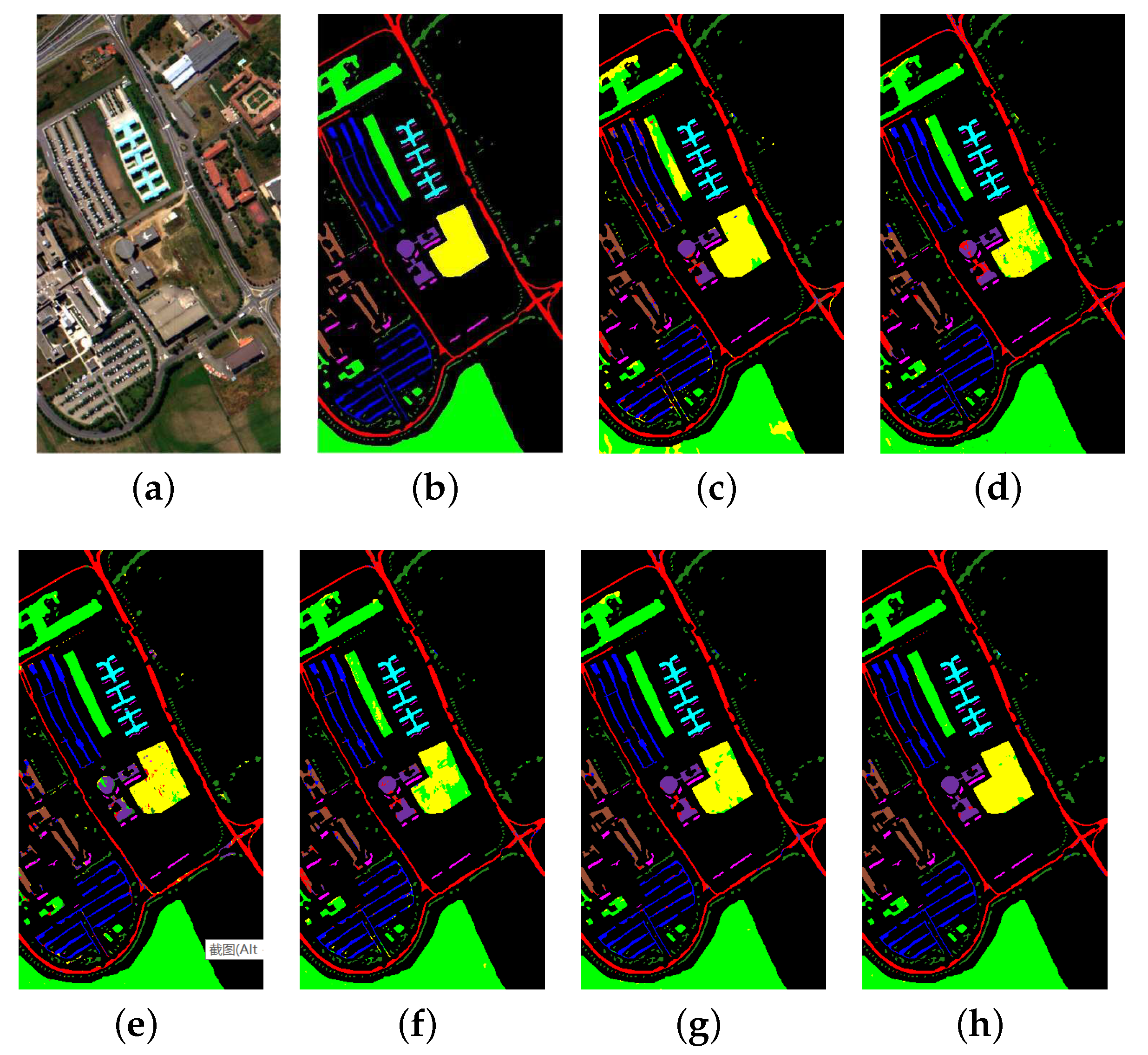
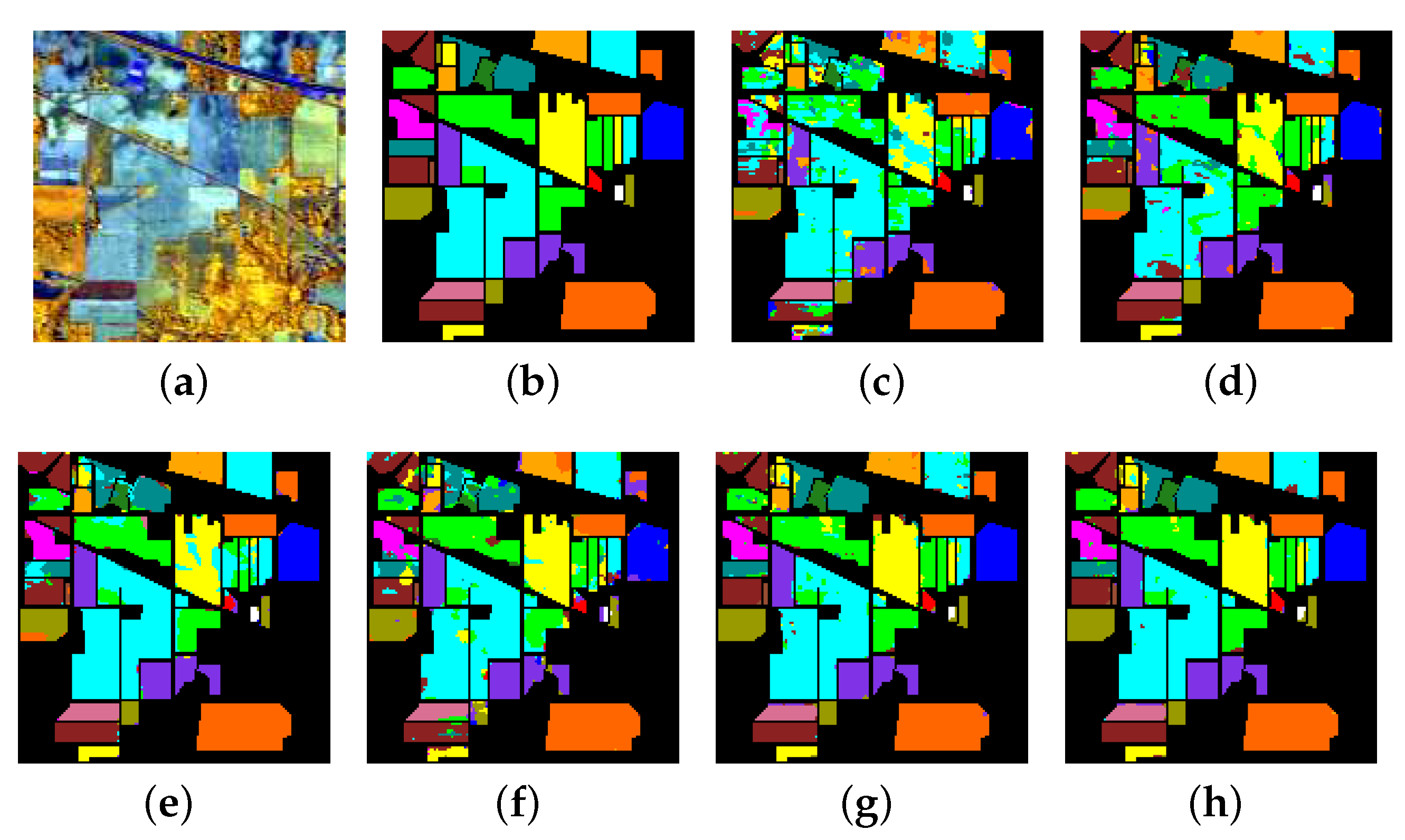
For better visual comparison, classification maps of Pavia University and Indian Pines obtained by different methods are depicted in Figure 10 and Figure 11, respectively.
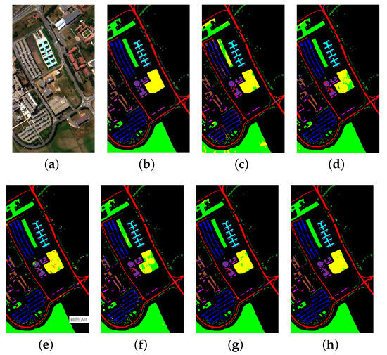
Figure 10.
Pavia University: (a) Composite image, (b) Ground truth, (c) FA, (d) DBN, (e) 2D-CNN, (f) SAE, (g) 3D-CAE (single-level features), and (h) 3D-CAE (multi-level features).

Figure 11.
Indian Pines: (a) Composite image, (b) Ground truth, (c) FA, (d) DBN, (e) 2D-CNN, (f) SAE, (g) 3D-CAE (single-level features), and (h) 3D-CAE (multi-level features).
For the Pavia University data set, it can be seen that there are many pixels in the green area that are incorrectly classified into the yellow. Some pixels in the sienna region are misclassified into the red in Figure 10c–e. Besides, the misclassified pixels in the green and sienna region are greatly reduced in Figure 10f,g, but some pixels in the purple region are still not correctly classified, especially in Figure 10e. Overall, the classification map in Figure 10h is the clearest.
For the Indian Pines data set, there are many misclassified pixels in Figure 11c,d,f,g, especially the upper left corner area. The classification maps in Figure 11e,f are better. Among all of the clasification maps, Figure 11f is the most satisfactory and it has the least number of misclassified pixels, which demonstrates the effectiveness of the proposed method.
5. Conclusions
In this paper, a 3D-CAE is designed to get rid of limitations of labeled samples. To fully exploit the spectral-spatial features of hyperspectral data, the 3D-CAE is stacked by 3D convolutional layers and 3D deconvolutional layers, so that 3D data blocks can be directly used as network input. Besides, multi-level features obtained from multiple encoded layers are developed to further improve classification accuracy in order to make full use of the well-trained network and retain as much feature information as possible.
Two commonly used hyperspectral data sets, Pavia University and Indian Pines, are used to verify the performance of the proposed method. Our experimental results show that single-level features from the top encoded layer perform better when compared to single-level features from other encoded layers. The performance of the proposed multi-level features exceeds any single-level features under different input sizes. The OA, AA, and values based on proposed multi-level features increased by about 2% to 3% for Pavia University and 2% to 5% for Indian Pines, as compared with single-level features from top encoded layer. Besides, we find that the number of layers used to form multi-level features also affects the feature performance. The more encoded layers are selected, the larger the dimension of the multi-level features. Our goal is to use low-dimensional features to obtain high accuracy. Based on our results, we choose three encoded layers for multi-layer features when the 3D-CAE has nine layers. Moreover, the proposed multi-level features are compared with the features obtained by supervised DBN and 2D-CNN, as well as unsupervised FA and SAE. The experimental results show that the proposed method outperforms the considered methods. The proposed multi-level features help us to obtain the highest classification accuracy, which demonstrates that they have huge potential in hyperspectral classification.
In summary, to solve the problem of limited labeled samples in HSIs, we design an unsupervised feature extraction network that is based on 3D-CAE. To make full use of the well-trained network and further improve feature quality, multi-level features are proposed to contain detail information and semantic information at the same time. The proposed multi-level features are directly obtained from different encoded layers of the optimized encoder, which is more efficient as compared to training multiple networks. It can also provide ideas for the full use of other deep learning models.
Author Contributions
Conceptualization, Q.S., X.L. and S.B.; Formal analysis, Q.S., X.L. and S.B.; Funding acquisition, X.L. and S.B.; Methodology, Q.S., X.L. and S.B.; Project administration, X.L. and S.B.; Software, Q.S.; Supervision, X.L. and S.B.; Validation, Q.S.; Writing—original draft, Q.S.; Writing—review and editing, X.L. and S.B. All authors have read and agreed to the published version of the manuscript.
Funding
This research was funded by the National Natural Science Foundation of China (Grant NO. 61971253, 61773227).
Institutional Review Board Statement
Not applicable.
Informed Consent Statement
Not applicable.
Data Availability Statement
Not applicable.
Acknowledgments
The authors would like to thank the reviewers for their careful reading and helpful comments which improve the quality of this paper.
Conflicts of Interest
The authors declare no conflict of interest.
References
- Scafutto, R.D.P.M.; de Souza Filho, C.R.; de Oliveira, W.J. Hyperspectral remote sensing detection of petroleum hydrocarbons in mixtures with mineral substrates: Implications for onshore exploration and monitoring. J. Photogramm. Remote Sens. 2017, 128, 146–157. [Google Scholar] [CrossRef]
- Delalieux, S.; Zarco-Tejada, P.J.; Tits, L.; Bello, M.Á.J.; Intrigliolo, D.S.; Somers, B. Unmixing-based fusion of hyperspatial and hyperspectral airborne imagery for early detection of vegetation stress. IEEE J. Sel. Top. Appl. Earth Observ. Remote Sens. 2014, 7, 2571–2582. [Google Scholar] [CrossRef]
- Chang, C.I. Hyperspectral Imaging: Techniques for Spectral Detection and Classification; Springer Science & Business Media: Berlin/Heidelberg, Germany, 2013. [Google Scholar]
- Tao, Y.; Xu, M.; Zhong, Y.; Cheng, Y. GAN-assisted two-stream neural network for high-resolution remote sensing image classification. Remote Sens. 2017, 9, 1328. [Google Scholar] [CrossRef]
- Anwar, S.M.; Majid, M.; Qayyum, A.; Awais, M.; Alnowami, M.; Khan, M.K. Medical image analysis using convolutional neural networks: A review. J. Med. Syst. 2018, 42, 226. [Google Scholar] [CrossRef]
- Gao, Q.; Lim, S.; Jia, X. Hyperspectral image classification using convolutional neural networks and multiple feature learning. Remote Sens. 2018, 10, 299. [Google Scholar] [CrossRef]
- Li, S.; Song, W.; Fang, L.; Chen, Y.; Ghamisi, P.; Benediktsson, J.A. Deep learning for hyperspectral image classification: An overview. IEEE Trans. Geosci. Remote Sens. 2019, 57, 6690–6709. [Google Scholar] [CrossRef]
- Otter, D.W.; Medina, J.R.; Kalita, J.K. A survey of the usages of deep learning for natural language processing. IEEE Trans. Neural Netw. Learn. Syst. 2020, 32, 604–624. [Google Scholar] [CrossRef]
- Guo, J.; He, H.; He, T.; Lausen, L.; Li, M.; Lin, H.; Shi, X.; Wang, C.; Xie, J.; Zha, S.; et al. GluonCV and GluonNLP: Deep Learning in Computer Vision and Natural Language Processing. J. Mach. Learn. Res. 2020, 21, 1–7. [Google Scholar]
- Young, T.; Hazarika, D.; Poria, S.; Cambria, E. Recent trends in deep learning based natural language processing. IEEE Comput. Intell. Mag. 2018, 13, 55–75. [Google Scholar] [CrossRef]
- Wu, S.; Roberts, K.; Datta, S.; Du, J.; Ji, Z.; Si, Y.; Soni, S.; Wang, Q.; Wei, Q.; Xiang, Y.; et al. Deep learning in clinical natural language processing: A methodical review. J. Am. Med. Inform. Assoc. 2020, 27, 457–470. [Google Scholar] [CrossRef] [PubMed]
- Zhao, Z.Q.; Zheng, P.; Xu, S.T.; Wu, X. Object detection with deep learning: A review. IEEE Trans. Neural Netw. Learn. Syst. 2019, 30, 3212–3232. [Google Scholar] [CrossRef]
- Yang, C.; Chen, J.; Li, Z.; Huang, Y. Structural Crack Detection and Recognition Based on Deep Learning. Appl. Sci. 2021, 11, 2868. [Google Scholar] [CrossRef]
- Li, K.; Zhang, K.; Zhang, Z.; Liu, Z.; Hua, S.; He, J. A UAV Maneuver Decision-Making Algorithm for Autonomous Airdrop Based on Deep Reinforcement Learning. Sensors 2021, 21, 2233. [Google Scholar] [CrossRef]
- Gadekallu, T.R.; Khare, N.; Bhattacharya, S.; Singh, S.; Reddy Maddikunta, P.K.; Ra, I.H.; Alazab, M. Early detection of diabetic retinopathy using PCA-firefly based deep learning model. Electronics 2020, 9, 274. [Google Scholar] [CrossRef]
- Li, Y.; Zhang, H.; Shen, Q. Spectral-spatial classification of hyperspectral imagery with 3D convolutional neural network. Remote Sens. 2017, 9, 67. [Google Scholar] [CrossRef]
- Chen, Y.; Jiang, H.; Li, C.; Jia, X.; Ghamisi, P. Deep feature extraction and classification of hyperspectral images based on convolutional neural networks. IEEE Trans. Geosci. Remote Sens. 2016, 54, 6232–6251. [Google Scholar] [CrossRef]
- Yu, C.; Han, R.; Song, M.; Liu, C.; Chang, C.I. A simplified 2D-3D CNN architecture for hyperspectral image classification based on spatial–spectral fusion. IEEE J. Sel. Top. Appl. Earth Observ. Remote Sens. 2020, 13, 2485–2501. [Google Scholar] [CrossRef]
- Zhan, Y.; Hu, D.; Wang, Y.; Yu, X. Semisupervised hyperspectral image classification based on generative adversarial networks. IEEE Geosci. Remote Sens. Lett. 2017, 15, 212–216. [Google Scholar] [CrossRef]
- Xie, F.; Gao, Q.; Jin, C.; Zhao, F. Hyperspectral Image Classification Based on Superpixel Pooling Convolutional Neural Network with Transfer Learning. Remote Sens. 2021, 13, 930. [Google Scholar] [CrossRef]
- Goodfellow, I.J.; Pouget-Abadie, J.; Mirza, M.; Xu, B.; Warde-Farley, D.; Ozair, S.; Courville, A.; Bengio, Y. Generative adversarial networks. arXiv 2014, arXiv:1406.2661. [Google Scholar]
- Liang, H.; Bao, W.; Shen, X. Adaptive Weighting Feature Fusion Approach Based on Generative Adversarial Network for Hyperspectral Image Classification. Remote Sens. 2021, 13, 198. [Google Scholar] [CrossRef]
- Radford, A.; Metz, L.; Chintala, S. Unsupervised representation learning with deep convolutional generative adversarial networks. arXiv 2015, arXiv:1511.06434. [Google Scholar]
- Zhang, M.; Gong, M.; Mao, Y.; Li, J.; Wu, Y. Unsupervised feature extraction in hyperspectral images based on wasserstein generative adversarial network. IEEE Trans. Geosci. Remote Sens. 2018, 57, 2669–2688. [Google Scholar] [CrossRef]
- Hu, A.; Xie, Z.; Xu, Y.; Xie, M.; Wu, L.; Qiu, Q. Unsupervised Haze Removal for High-Resolution Optical Remote-Sensing Images Based on Improved Generative Adversarial Networks. Remote Sens. 2020, 12, 4162. [Google Scholar] [CrossRef]
- Vincent, P.; Larochelle, H.; Lajoie, I.; Bengio, Y.; Manzagol, P.A.; Bottou, L. Stacked denoising autoencoders: Learning useful representations in a deep network with a local denoising criterion. J. Mach. Learn. Res. 2010, 11, 3371–3408. [Google Scholar]
- Protopapadakis, E.; Doulamis, A.; Doulamis, N.; Maltezos, E. Stacked Autoencoders Driven by Semi-Supervised Learning for Building Extraction from near Infrared Remote Sensing Imagery. Remote Sens. 2021, 13, 371. [Google Scholar] [CrossRef]
- Tao, C.; Pan, H.; Li, Y.; Zou, Z. Unsupervised spectral-spatial feature learning with stacked sparse autoencoder for hyperspectral imagery classification. IEEE Geosci. Remote Sens. Lett. 2015, 12, 2438–2442. [Google Scholar]
- Zhou, P.; Han, J.; Cheng, G.; Zhang, B. Learning compact and discriminative stacked autoencoder for hyperspectral image classification. IEEE Trans. Geosci. Remote Sens. 2019, 57, 4823–4833. [Google Scholar] [CrossRef]
- Zhang, X.; Liang, Y.; Li, C.; Huyan, N.; Jiao, L.; Zhou, H. Recursive autoencoders-based unsupervised feature learning for hyperspectral image classification. IEEE Geosci. Remote Sens. Lett. 2017, 14, 1928–1932. [Google Scholar] [CrossRef]
- Mei, S.; Ji, J.; Geng, Y.; Zhang, Z.; Li, X.; Du, Q. Unsupervised spatial–spectral feature learning by 3D convolutional autoencoder for hyperspectral classification. IEEE Trans. Geosci. Remote Sens. 2019, 57, 6808–6820. [Google Scholar] [CrossRef]
- Lin, T.Y.; Dollár, P.; Girshick, R.; He, K.; Hariharan, B.; Belongie, S. Feature pyramid networks for object detection. In Proceedings of the IEEE Conference on Computer Vision and Pattern Recognition, Honolulu, HI, USA, 21–26 July 2017; pp. 2117–2125. [Google Scholar]
- Adelson, E.H.; Anderson, C.H.; Bergen, J.R.; Burt, P.J.; Ogden, J.M. Pyramid methods in image processing. RCA Eng. 1984, 29, 33–41. [Google Scholar]
- Tran, D.; Bourdev, L.; Fergus, R.; Torresani, L.; Paluri, M. Learning spatiotemporal features with 3d convolutional networks. In Proceedings of the IEEE International Conference on Computer Vision, Santiago, Chile, 13–16 December 2015; pp. 4489–4497. [Google Scholar]
- Zuo, Z.; Shuai, B.; Wang, G.; Liu, X.; Wang, X.; Wang, B.; Chen, Y. Learning contextual dependence with convolutional hierarchical recurrent neural networks. IEEE Trans. Image Process. 2016, 25, 2983–2996. [Google Scholar] [CrossRef] [PubMed]
- Agarwal, A.; El-Ghazawi, T.; El-Askary, H.; Le-Moigne, J. Efficient hierarchical-PCA dimension reduction for hyperspectral imagery. In Proceedings of the IEEE International Symposium on Signal Processing and Information Technology, Giza, Egypt, 15–18 December 2007; pp. 353–356. [Google Scholar]
- Zhu, L.; Chen, Y.; Ghamisi, P.; Benediktsson, J.A. Generative adversarial networks for hyperspectral image classification. IEEE Trans. Geosci. Remote Sens. 2018, 56, 5046–5063. [Google Scholar] [CrossRef]
- Kingma, D.P.; Ba, J. Adam: A method for stochastic optimization. arXiv 2014, arXiv:1412.6980. [Google Scholar]
- Liu, Y.; Zhou, S.; Chen, Q. Discriminative deep belief networks for visual data classification. Pattern Recognit. 2011, 44, 2287–2296. [Google Scholar] [CrossRef]
- Abdel-Zaher, A.M.; Eldeib, A.M. Breast cancer classification using deep belief networks. Expert Syst. Appl. 2016, 46, 139–144. [Google Scholar] [CrossRef]
- Li, J.; Xi, B.; Li, Y.; Du, Q.; Wang, K. Hyperspectral classification based on texture feature enhancement and deep belief networks. Remote Sens. 2018, 10, 396. [Google Scholar] [CrossRef]
- Attias, H. Independent factor analysis. Neural Comput. 1999, 11, 803–851. [Google Scholar] [CrossRef]
- Kang, M.; Ji, K.; Leng, X.; Xing, X.; Zou, H. Synthetic aperture radar target recognition with feature fusion based on a stacked autoencoder. Sensors 2017, 17, 192. [Google Scholar] [CrossRef]
- Liang, P.; Shi, W.; Zhang, X. Remote sensing image classification based on stacked denoising autoencoder. Remote Sens. 2018, 10, 16. [Google Scholar] [CrossRef]
Publisher’s Note: MDPI stays neutral with regard to jurisdictional claims in published maps and institutional affiliations. |
© 2021 by the authors. Licensee MDPI, Basel, Switzerland. This article is an open access article distributed under the terms and conditions of the Creative Commons Attribution (CC BY) license (https://creativecommons.org/licenses/by/4.0/).

