Article

Tree Crowns Cause Border Effects in Area-Based Biomass Estimations from Remote Sensing

1
Department of Ecological Modelling, Helmholtz Centre for Environmental Research—UFZ, 04318 Leipzig, Germany
2
German Centre for Integrative Biodiversity Research (iDiv), Halle-Jena-Leipzig, 04103 Leipzig, Germany
3
Institute of Environmental Systems Research, University Osnabrück, 49076 Osnabrück, Germany
*
Author to whom correspondence should be addressed.
Remote Sens. 2021, 13(8), 1592; https://doi.org/10.3390/rs13081592
Submission received: 11 February 2021 / Revised: 11 March 2021 / Accepted: 14 April 2021 / Published: 20 April 2021
(This article belongs to the Special Issue Remote Sensing Models of Forest Structure, Composition, and Function)

Abstract

:
The estimation of forest biomass by remote sensing is constrained by different uncertainties. An important source of uncertainty is the border effect, as tree crowns are not constrained by plot borders. Lidar remote sensing systems record the canopy height within a certain area, while the ground-truth is commonly the aboveground biomass of inventory trees geolocated at their stem positions. Hence, tree crowns reaching out of or into the observed area are contributing to the uncertainty in canopy-height–based biomass estimation. In this study, forest inventory data and simulations of a tropical rainforest’s canopy were used to quantify the amount of incoming and outgoing canopy volume and surface at different plot sizes (10, 20, 50, and 100 m). This was performed with a bottom-up approach entirely based on forest inventory data and allometric relationships, from which idealized lidar canopy heights were simulated by representing the forest canopy as a 3D voxel space. In this voxel space, the position of each voxel is known, and it is also known to which tree each voxel belongs and where the stem of this tree is located. This knowledge was used to analyze the role of incoming and outgoing crowns. The contribution of the border effects to the biomass estimation uncertainty was quantified for the case of small-footprint lidar (a simulated canopy height model, CHM) and large-footprint lidar (simulated waveforms with footprint sizes of 23 and 65 m, corresponding to the GEDI and ICESat GLAS sensors). A strong effect of spatial scale was found: e.g., for 20-m plots, on average, 16% of the CHM surface belonged to trees located outside of the plots, while for 100-m plots this incoming CHM fraction was only 3%. The border effects accounted for 40% of the biomass estimation uncertainty at the 20-m scale, but had no contribution at the 100-m scale. For GEDI- and GLAS-based biomass estimates, the contributions of border effects were 23% and 6%, respectively. This study presents a novel approach for disentangling the sources of uncertainty in the remote sensing of forest structures using virtual canopy modeling.

Graphical Abstract

1. Introduction

Biomass maps derived from remote sensing methods are an effective way to conduct detailed, spatially explicit carbon accounting of vegetation over large areas. They are crucial for the understanding of the global carbon budget and for quantifying the CO2 sequestration by forests [1]. In recent years, considerable effort has been made to improve forest biomass mapping approaches and to generate maps with increasing spatial resolutions. A frequently applied method for aboveground biomass (AGB) estimation uses remote sensing data from active sensor systems, such as light detection and ranging (lidar) or synthetic aperture radar [2]. Such data are used to generate metrics of canopy height, which are linked to AGB via regression models [3]. Canopy height metrics and AGB are calculated in an area-based way, i.e., representing the whole forest over a certain area, and not at the individual tree level [4]. The area sizes used depend on the size of the available ground-truth plots for the calculation of the reference AGB, the footprint size of the lidar system, or the desired resolution of the produced AGB map [5].
The AGB of single trees in the ground-truth plots is commonly geolocated at their stem positions. This is done mostly for practical reasons, but it can also be justified structurally because most of a tree’s AGB is contained in the stem. The canopy height metrics, on the other hand, are calculated from the remote sensing signal, which results from reflections from the tree crowns. The tree crowns cover a certain spatial extent around the stem positions. Hence, there is a spatial mismatch between the remote sensing metrics and the ground-truth [6]. As long as the entire tree crown is contained within the considered plot area, this mismatch does not pose a problem. However, at the borders of plots, tree crowns can reach out of the plot (outgoing crowns) and crowns from outside trees can reach into the plot (incoming crowns). These outgoing and incoming crowns affect the values of the canopy height metrics calculated for the plot, while for the ground-truth AGB calculation the plot borders are strict borders, and only tree stems inside the plot are considered, independent of their crown extension [6,7]. The uncertainty in the height–biomass relationship caused by incoming and outgoing tree crowns is referred to as a ‘border effect’. Other studies have also called it an ‘edge effect’, but because this term in forest ecology is often understood as the effects leading to altered forest dynamics near forest edges [8], we chose here to use the term ‘border effect’ to avoid misunderstandings.
The proportion of incoming and outgoing tree crowns is expected to be larger the smaller the plot sizes are. In general, it has been found that uncertainties in biomass estimation at the single-plot level increase with decreasing plot size, which is usually observed as an increase in the root mean square error and a decrease in the R² for biomass estimates [5,6,9,10,11]. This means that area-based biomass maps cannot be produced at arbitrarily fine resolutions without generating large uncertainties at the level of the single estimates. Border effects are thought to be one major contribution to this uncertainty. In order to better understand their contribution, it is important to have an idea about the magnitude of the incoming and outgoing crown volume and surface. Quantifying these proportions with empirical data is difficult because it would require a large number of crown measurements. Alternatively, the proportions can be analyzed using allometric assumptions and simulations in combination with forest inventory data [7,11,12]. Simulations have the additional advantage that the border effects can be switched off in the biomass estimation in order to quantify the residual uncertainty in the height–biomass relationship in an ideal situation where border effects do not exist. This can be achieved by enforcing periodic boundary conditions on the simulated tree crowns. Periodic boundaries are a common concept in ecological modeling, which are used to avoid edge effects in simulations [13]. They imply that the modelled area corresponds to a torus, which cannot be left. If something leaves the modelled area on one side it reappears on the opposite side. For the simulated tree crowns in this study, this means that the crowns which leave the plot on one end reappear on the opposite side, while no crowns from trees which are outside the plot are allowed to enter. With this approach, idealized analyses can be conducted, wherein the simulated remote sensing signal is generated exclusively (no incoming crowns) and entirely (if outgoing, then reappearing) by the crowns of trees which have their stem position inside the plot. This idealized approach helps to investigate the pure influence of the border effect on lidar-derived biomass estimates.
In this study, such simulations were conducted for a tropical rainforest in Panama using different plot sizes and shapes, including the circular footprints of the spaceborne lidars ICESat GLAS (65 m diameter) [14,15] and GEDI (23 m diameter) [16], in order to answer the following two questions: (1) How large are the proportions of the incoming and outgoing crown volume and canopy surface at different scales? (2) What is the contribution of border effects to the uncertainty in AGB estimations at different scales?

2. Materials and Methods

2.1. Dataset and Allometric Assumptions

Data from the Barro Colorado Island (BCI) 50-ha plot were used [17,18,19,20,21]. Located in central Panama at 9.15°N and 79.85°W, BCI is a neotropical moist lowland old-growth forest site. It has served as a research site for tropical ecology for several decades. Because of the large continuous inventory dataset, several studies about forest structure and biomass estimation from lidar have been conducted for BCI [6,22,23,24]. In this study, the census data from 2010 were used, which comprises 246,913 trees with a minimum diameter at breast height (DBH) of 1 cm. For each tree, the position within the plot was recorded. The tree height, crown diameter and aboveground biomass were calculated for each tree as follows. The tree height H was calculated from DBH (in m units) using a Michaelis–Menten Equation (1).
H = 57.4 · DBH 0.43 + DBH
The crown diameter CD was calculated from DBH using a power law Equation (2).
CD = 15.55 · DBH 0.68
The parameters for Equations (1) and (2) were derived by fitting regression models to a dataset of 12,348 neotropical trees with measured attributes [25] (subset: functional type “Angio”, biogeographic zone “Neotropic”, biome “Tropical forests”). In order to analyze how the variability in the crown diameter allometry might affect the results, we repeated parts of the analysis with randomly altered crown diameters according to Equation (3).
CD = 15.55 · DBH 0.68 · ( 1 + ε ) ;   ε   ~   Norm ( μ = 0 ,   σ = 0.39 )
The random variability ε was modelled as a normal distribution, for which the standard deviation (σ = 0.39) was derived from the residuals of Equation (2) with respect to the 12,348 trees in the dataset [25]. The normal distribution was truncated at the 95% prediction intervals (±1.96·σ) in order to avoid negative and unrealistically large crown diameter values. The crown length was calculated as 0.4 times tree height [11]. For each tree, a leaf area index of 2 was assumed, which—in combination with the crown volume—allowed the calculation of the leaf area density. These assumptions about crown length and leaf area density have proven suitable for forest and lidar simulations for BCI before [11]. The aboveground biomass of each single tree (AGBtree) was calculated using a generic tropical tree biomass allometry (Equation (4) corresponding to “Model 5” from [26]) with the DBH, estimated tree height H, and wood density WD of the species [27] as inputs.
AGB tree = 0.559 ·   DBH 2   ·   H   ·   WD

2.2. Voxel Forest Generation

The geometrical information of every tree was used to construct a three-dimensional representation of the forest stand assuming spheroid tree crowns (equally elongated in the X and Y directions but different in the Z direction) based on the inventory dataset. The spatial resolution of the voxels in 3D space was 1 m × 1 m × 1 m. The voxel forest was stored as a data table with rows representing tree crown voxels. The columns contained the X, Y and Z coordinates of the voxels, the leaf area density, and additional information about the tree to which the voxel belongs (e.g., tree ID, X and Y position of the stem). Knowing, for each voxel, the coordinates and also the position of the associated stem was a requirement for the later analysis of incoming and outgoing crowns.
A subset of the data table was stored representing only the upper surfaces of the tree crowns which are visible from above (i.e., the voxel with the maximal Z value for each unique combination of X and Y). Raster representations of the upper canopy surface are commonly called canopy height models (CHM). They can be derived from lidar point clouds, photogrammetry, or radar. CHMs from airborne lidar are commonly derived with a simple point-to-raster method for dense point clouds, or via interpolation methods for less dense point clouds [28]. Hence, rasterizing the maximal Z value for each unique X and Y combination in our 3D voxel space leads to a simulated CHM of 1-m resolution, which is entirely based on the inventory data and allometric relationships. Because, for the simulated lidar, there is no geolocation error with respect to the inventory, the pure border effect can be studied.

2.3. Crown Space Quantification

For different plot sizes, it was analyzed which proportion of the tree crowns over a plot is incoming (i.e., belongs to trees that stand outside the plot area) and which proportion of tree crowns of the trees on the plot is outgoing (i.e., falls outside the plot area). For this purpose, the 50-ha plot was divided into subplots with side lengths of 10, 20, 50 and 100 m, respectively. For each plot size, each voxel was labeled with (a) a plot ID of the voxel’s X and Y position, and (b) a plot ID of the corresponding tree stem’s X- and Y-position. This allowed us to easily distinguish between voxels which are located over the same plot as their tree stems and voxels which are located over a plot other than the plot of their tree stems.
For each plot at each scale, the following quantities were computed by counting the respective numbers of 1-m³ voxels: (1) the total crown volume of all of the trees standing inside a plot (CVt); (2) the total crown volume that is exactly above the plot (CVp); (3) the crown volume that fulfills both of the previous conditions, i.e., the voxel is above the plot and the tree stem is inside the plot (CVt&p); (4) the incoming crown volume (CVin = CVp − CVt&p); (5) the outgoing crown volume (CVout = CVt − CVt&p); (6) the total canopy surface of all trees standing on a plot (CSt); (7) the total canopy surface that is exactly above the plot (CSp); (8) the canopy surface that fulfills both of the previous conditions, i.e., the surface is above the plot and the tree stem is inside the plot (CSt&p); (9) the incoming canopy surface (CSin = CSp − CSt&p); (10) the outgoing canopy surface (CSout = CSt − CSt&p). The means and ranges of these quantities were calculated for each spatial scale. Figure 1 illustrates some of these quantities.

2.4. Biomass Estimation Using Square Plots and CHM

The area-based biomass estimation from simulated lidar CHMs was tested at the different plot sizes. The AGB per plot was calculated as the AGB sum of all of the trees standing inside each square-shaped plot of 10, 20, 50 and 100 m side length, and was rescaled to t ha−1 units. The subset of voxels which represent the canopy surface was interpreted as a 1-m resolution CHM (as typically derived from small footprint discrete return lidar). The mean top-of-canopy height (TCH) was calculated by averaging the heights of all of the CHM pixels over each plot. Power law regression models describing AGB as a function of TCH (Equation (5)) were fitted using maximum likelihood estimation in R [29].
AGB = a   ·   TCH b

2.5. Biomass Estimation Using Large-Footprint Lidar

Large-footprint lidar waveforms were simulated to derive the mean canopy profile height (MCH) and link it to the AGB in the footprint. Unlike in the case of the CHM, in which only the voxels of the canopy surface were considered, for the waveform simulations all of the canopy voxels and also the ground voxels falling into the circular footprint areas were considered. The contribution of a voxel to the simulated waveform depended on three factors: (1) the number of crown voxels above, to account for light extinction in the canopy; (2) the distance to the footprint center, to account for the Gaussian energy distribution within a laser beam; and (3) the fact of whether the voxel was located in the canopy or on the ground. Figure 2 illustrates the waveform simulation for an example transect across a 65-m diameter footprint. Equation (6) describes the calculation of the lidar intensity I of each voxel (i.e., its contribution to the lidar waveform) mathematically. A voxel at the canopy surface and in the center of the footprint is assumed to contribute the highest possible intensity. If a voxel is further down in the canopy or more distant from the footprint center, its contribution to the reflected signal is reduced.
I = e k   ·   LAI + d 2 2   ·   SD 2
Light extinction was modelled using Beer–Lambert’s law, with e being the base of the natural logarithm. The light extinction coefficient k was set to 0.2 [11]. LAI is the leaf area index above the voxel, calculated as the sum of the leaf area densities of all of the voxels lying directly above (same X and Y coordinate). The Gaussian energy distribution was modelled by the quotient term in the exponent of Equation (6), where d is the distance of the voxel to the footprint center in the XY-plane, and SD is the standard deviation of the Gaussian distribution, which was set to 0.5 times the footprint radius [30]. The reflectance of the forest ground voxels was down-weighted by dividing by 2.5 in order to account for the lower reflectivity of the ground vs. vegetation [31]. The reflected intensities of all of the voxels in each 1-m height layer were summed up and the waveforms were standardized to have a total sum of one (Figure 2).
Waveforms were simulated for footprints of 23 m (GEDI) and 65 m (ICESat GLAS) diameters. A total of 171 footprints of each type were placed at 50 m regular spacing inside the 50-ha plot (Figure A1). The AGB per footprint was calculated as the AGB sum of all of the trees standing inside the footprint circle. The mean canopy profile height (MCH) was calculated as the intensity-weighted mean height of the waveform. Power law regression models describing AGB as a function of MCH (Equation (7)) were fitted using maximum likelihood estimation in R.
AGB = a   ·   MCH b

2.6. Uncertainty Quantification

The uncertainty in the AGB estimation was quantified by comparing predictions (AGBpred) derived from the power law regression models against observations (AGBobs). AGBobs were the plot-level sums over all of the AGBtree (Equation (4)) values of the trees inside a plot. The AGBobs were rescaled to t ha−1 units for all of the plot sizes. The calculated statistics were the coefficient of determination (R²), the root mean square error (RMSE, Equation (8)) and the normalized root mean square error (nRMSE, Equation (9)), with i representing each plot and n representing the total number of plots.
RMSE = 1 n · i = 1 n ( AGB pred ,   i AGB obs ,   i ) 2
nRMSE = 1 n × i = 1 n ( AGB pred ,   i   AGB obs ,   i ) 2 1 n · i = 1 n AGB obs ,   i

2.7. Periodic Boundary Conditions

In order to quantify the contribution of border effects to the uncertainty in AGB estimation, periodic boundary conditions were applied to the plots (Figure 3). Under these conditions, all of the original incoming voxels, i.e., the voxels belonging to trees which have their stem outside of the focal plot, were removed. On the other hand, outgoing voxels—i.e., voxels belonging to trees which have their stem inside the focal plot, but are themselves outside the plot—were shifted to the opposite side of the plot. Hence, the new incoming crown voxels are the ones which are outgoing on the other side. As a visual example, consider the large orange colored tree located in the middle of the 1-ha forest area displayed in Figure 3c. Its stem (and crown center) is located in the central 20-m plot, but parts of its crown are outgoing, i.e., they extend into three other plots (the left, top and top-left neighbor). After enforcing periodic boundaries, these crown parts reappear in the focal plot (from the right and bottom side and bottom-right corner, respectively; Figure 3d). For the straight borders of the square-shaped plots, the establishment of the periodic boundaries was realized by adding (left or bottom border) or subtracting (right or top border) one plot width from the X or Y coordinates of the outgoing crown voxels, respectively. For the curved borders of circular footprints there is no exact correspondence. The following solution was applied in order to generate quasi-periodic boundaries for the circular footprints: for all of the trees with stems inside the circle, virtual twins were created by copying them to exist a second time outside of the circle at the position opposite to the circle center and with the same distance to the boundary, but outwards. Then, the crown voxels falling into the circle area were selected to simulate the waveforms, as described in Section 2.5 and Figure 2.
The uncertainty in the biomass estimation was quantified for the different plot sizes and shapes. Firstly, the uncertainty was quantified under normal conditions, where incoming and outgoing crowns disturb the height–biomass relationship. Secondly, the uncertainty was quantified under periodic boundary conditions, where border effects are non-existent. The difference in the nRMSE between the normal and periodic boundary conditions was used to quantify the contribution of the border effect. When this difference is divided by the overall nRMSE, the relative contribution of the border effect can be obtained. Please note, both quantities—nRMSE and the relative contribution of the border effect to the nRMSE—are given in %-units.

3. Results

3.1. Proportions of Incoming and Outgoing Crowns

The analysis showed that, in small forest plots, a considerable proportion of the crown space was either incoming or outgoing. As expected, this proportion decreased with an increasing plot size. Table 1 summarizes the observed mean and maximum values for different proportions at the investigated spatial scales (standard deviations are given in Table A1). The outgoing crown volume is presented as a proportion of the crown volume of all of the trees with stems on the plot (CVout/CVt). The incoming crown volume is likewise presented as proportion of the crown volume of all of the trees with stems on the plot (CVin/CVt). This ratio can be larger than one, and can take on quite high values, because (unlike CVout) CVin is not a subset of CVt. Thus, it is more meaningful to quantify the incoming volume as a proportion of the crown volume which is exactly located above the plot (CVin/CVp). The canopy surface areas CSin and CSout are both presented as proportions of the plot area.
There was a close similarity between the proportions of the incoming/outgoing crown volume and the incoming/outgoing canopy surface. At the 10-m scale, ~30% of CV and CS were incoming and outgoing, respectively. The proportions decreased to half the size (~15%) when doubling the plot side length (20 m) and decreased to one tenth (~3%) for the ten-fold plot side length (100 m, 1-ha plots).
The maxima of the incoming/outgoing crown volume were quite large. At the 10-m scale, in the most extreme cases, CVin contributed up to 95% of CVp and exceeded CVt by a factor 16. Such cases occur if the focal plot contains only very small trees with a small total crown volume and large trees from a neighboring plot dominate the canopy over the focal plot.
In the case of the canopy surface, at a 10-m scale, the CHM of the plot can be entirely formed by the incoming surface, and the outgoing canopy surface can exceed the plot size by a factor 6 due to the fact that single-tree crown projection areas can be far larger than the plot size (the maximum crown diameter 28.8 m corresponding to a 652 m² crown projection area). At the 100-m scale, the maxima of all of the investigated proportions were ≤7%.
When the variability in the crown diameters was included in the analysis (using Equation (3) instead of (2)), most of the proportions listed in Table 1 slightly increased (Table 2). This was expected, because introducing variability to crown diameters will lead to more crown volume overall, as the three-dimensional volumes are calculated based on the one-dimensional diameters. There are two concerns about including the variability: Firstly, it represents the variability of neotropical broadleaf rainforest trees in the database by [25], which is expected to be higher than the variability on BCI alone. Secondly, the variability in the crown shape is largely driven by competition for space among tree individuals, which was not accounted for in the simulations. For all of the further analyses, the crown diameters from the average allometry (Equation (2)) were used.

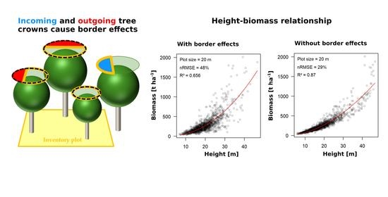
3.2. Biomass Estimation Results Using Square Plots and CHM

The biomass estimation uncertainty decreased strongly with the increasing plot size. The contribution of border effects also decreased with increasing plot size (Figure 4). At the 10-m scale, the overall nRMSE was 121%, with a contribution of 53% caused by border effects, and a residual nRMSE of 68% when border effects were excluded by periodic boundary conditions. At the 20-m scale, the overall nRMSE was 48%, of which 19% could be attributed to border effects and 29% was residual uncertainty. At the 50-m scale, the overall nRMSE was 17%, with 5% being contributed by border effects and 12% being residual uncertainty. At the 100-m scale, border effects became negligible, with an overall nRMSE of 7%, which did not decrease under periodic boundary conditions. Hence, the relative contributions of the border effect to the overall uncertainty were 44%, 40%, 29% and 0% at the 10-, 20-, 50- and 100-m scales, respectively (Table 3). The R² values increased from 0.49 to 0.86 with the increasing scale, while under periodic boundary conditions they were ≥0.85 at all of the scales.

3.3. Biomass Estimation Results Using Large-Footprint Lidar

The effect of spatial scale could also be observed for the waveform-based biomass estimations in the circular footprints. A larger footprint size resulted in a smaller overall uncertainty in the biomass estimation, as well as a smaller contribution of the border effect (Figure 5). At the scale of a GEDI footprint (23 m), the overall nRMSE was 52%, with 12% being attributable to border effects and 40% being residual uncertainty. At the scale of an ICESat GLAS footprint (65 m), the overall nRMSE was 15%, with only 1% being attributable to border effects and 14% being residual uncertainty. Hence, the relative contributions of the border effect to the overall uncertainty were 23% at the GEDI scale and 6% at the GLAS scale (Table 3). The R² values were 0.54 and 0.7 at the GEDI and GLAS scales, respectively, while under periodic boundary conditions they were ≥0.72 in both cases.
The scaling behavior of the nRMSE for the different approaches is summarized in Figure 6. The distances between the black filled and grey open symbols show the contributions of the border effect to the AGB estimation at the different spatial scales, and where the waveform-based estimates lie in comparison to the CHM-based estimates at similar scales.

3.4. Effects of the Gaussian Energy Distribution

The Gaussian horizontal energy distribution within the laser beam has the effect that the tree crowns in the margins of the footprints contribute less to the signal than the tree crowns in the center. In order to test the magnitude of this effect, the simulations were also conducted without Gaussian weighting (Figure A2). Without Gaussian weighting, the relative contributions of the border effect to the overall uncertainty were 28% (instead of 23%) for GEDI and 17% (instead of 6%) for GLAS (Table 3).
Please note that, under periodic boundary conditions, the R2 values were almost equal across all of the scales. Hence, despite the observed scale dependence of the uncertainties (nRMSE), the strengths of the relationships between the predicted and observed biomass were scale independent in the absence of border effects. These R2 values were larger for the CHM-based estimates on square plots (~0.85, Figure 4b,d,f,h) than for the large-footprint waveform-based estimates (~0.72, Figure 5b,d). The weaker R2 for the waveform-based estimates can be explained by the fact that, for CHM-based estimates, the positions of the trees per se do not play a role. The CHM is a continuous and homogeneous sample of the canopy across the whole plot area. On the contrary, in the case of Gaussian energy distribution within a large lidar footprint, the signal contribution of each tree strongly depends on its position. Trees in the center of the footprint contribute more to the signal than trees near the border of the footprint. These differences are not considered in the calculation of the ground-truth AGB. This interpretation is in line with the fact that the R2 became higher when Gaussian weighting was switched off (0.75 and 0.87, Figure A2b,d). Hence, in biomass estimation from large-footprint lidar, the Gaussian weighting has two effects: it reduces the uncertainty due to border effects, but increases the uncertainty due to the unequal signal contribution from the central and marginal parts of the footprint. This explains why, at the small scale of GEDI footprints, where border effects are strong, the nRMSE increased slightly when Gaussian weighting was switched off (from 52 to 53%, Table 3). At the larger scale of the GLAS footprint, at which border effects are weak, the nRMSE decreased slightly when Gaussian weighting was switched off (from 15 to 12%, Table 3) because of the equal signal contribution from the entire footprint area.

4. Discussion

The role of border effects in forest remote sensing was investigated for a tropical forest in Panama. We quantified what proportion of the tree crown volume and observed canopy surface does not belong to trees standing inside plots, and how this proportion depends on the plot size. While at small scales, e.g., 10 m, on average, large proportions of the canopy volume and surface were incoming and outgoing (~30%), these average proportions became small at the 100-m scale (~3%). This is explained by the smaller perimeter-to-area ratio of the larger plots.
We further analyzed the ways in which border effects affect biomass estimation based on a CHM or large-footprint lidar waveforms. The incoming and outgoing tree crowns influence the quality of the derived relationship between the canopy height and the biomass. Hence, the smaller the proportion of incoming and outgoing crowns, i.e., the larger the plot area, the smaller the uncertainty in the biomass estimations should be. The observed uncertainties in the biomass estimations decreased with increasing plot sizes. While at 10- and 20-m scale, the border effect was responsible for ≥40% of the overall uncertainty, it had a contribution of 29% at the 50-m scale, and it had zero contribution at the 100-m scale. For the spaceborne large-footprint lidar systems, the border effect was responsible for 23% of the uncertainty in GEDI-based biomass estimates, and for 6% of the uncertainty in the ICESat GLAS-based biomass estimates.
The trend of increasing uncertainty with decreasing plot size was reported in previous studies [5,6,9,10,11]. It has partly been attributed to geolocation errors, which have smaller impacts if the plots are large [7,33], but this source of error can be ruled out in controlled simulation experiments. It is partly an effect of spatial averaging, i.e., the variability of individual trees becomes less important when aggregating over larger areas. It was found that the perimeter-to-area ratio of the plots/footprints, rather than their area alone, is a major factor in this trend [34]. The explanation behind this is the border effect, which is supported by our results.
The strengths of the border effects are influenced by several factors, including the size and shape of plots/footprints and the energy distribution within them. Under the assumption of an equal square plot and footprint size, it is expected that the border effects are smaller for the large-footprint lidar for two reasons: (1) the smaller perimeter-to-area ratio of circles compared to squares, and (2) the Gaussian horizontal energy distribution within the laser beam, which lowers the contribution of the canopy space in the footprint margins. In this study, CHM-based and waveform-based estimation were not compared directly using equal plot sizes, but the described effect becomes obvious when comparing the results of the 50-m plots (2500 m2 area) to the ones of the much smaller GEDI footprints (415 m2 area) and the only slightly larger GLAS footprints (3318 m2 area). The overall biomass uncertainty between 50-m square plots and GLAS was similar (18% and 15% nRMSE) but the relative contribution of border effects was much stronger for the 50-m square plots (29% vs. 6%). Even for the much smaller GEDI footprints, for which the overall uncertainty was three times higher (52% nRMSE), the relative contribution of the border effect was smaller (23%) than for the 50-m square plots (29%). Switching off the Gaussian energy distribution increased the contributions of border effects (from 23% to 28% for GEDI; from 6% to 17% for GLAS). Thus, the Gaussian energy distribution can be considered beneficial in the sense that it reduces the magnitude of border effects, but at the same time the unequal signal contribution of trees inside the footprint (central vs. marginal position) leads to a weaker height–biomass relationship, as was shown by the R2 values. These findings can provide guidance about choosing the proper scales for minimizing border effects in biomass mapping. However, choices are constrained, because wall-to-wall maps by definition have square-shaped pixels (or in rare cases hexagonal [35], but never circular pixels) and laser beams, by design, have circular cross-sectional areas with Gaussian energy distribution.
It should be mentioned that the results of this study were derived using general allometries for neotropical trees [25]. Because these trees can grow to very large crown sizes, and because the site is an old growth forest, the reported incoming and outgoing crown fractions and the border effect contributions are probably at the high end of values when compared with other forest types worldwide. In temperate and boreal forests—particularly those with coniferous trees, which often have more slender crowns—these fractions and contributions may be smaller. On the other hand, the experiment regarding the introduction of variability into the crown allometry has shown that border effects might even be slightly stronger than those derived by using the average allometric relation.
The finding that border effects no longer play a role at scales ≥1 ha is in accordance with previous work. Mascaro et al. [6] drew similar conclusions using a different approach, wherein they introduced the concept of crown-distributed—instead of stem-localized—biomass for the reference ground truth. For high-resolution discrete lidar data, border effects could be avoided by using biomass estimation methods based on individual tree crown delineation. Such approaches allow us to produce very high (e.g., 1-m) resolution biomass maps from lidar that closely resemble crown-distributed biomass maps from ground inventory [36]. However, individual-based approaches are not applicable over large areas with current technology, due to limitations in data acquisition and distribution and computational capacities [37]; in particular, the waveforms produced by spaceborne lidar systems require area-based interpretations.
Simulation studies, like the one presented here, can help to disentangle the contributions of various sources of uncertainty in remote sensing interpretation, including the border effect, but also others. Previous studies using similar approaches have already analyzed geolocation-induced uncertainty [7] and allometry-induced and structure-induced uncertainty [38]. Future studies could include all of these aspects simultaneously in order to analyze the combined uncertainty and then partition it into its components. More generally, such simulations may serve as a method for the fusion of remote sensing data with dynamic forest models [39], which enables new interpretations of remote sensing products for forest structure [40] and new possibilities for model and allometry calibration [12,41].

5. Conclusions

Quantifying the fractions of incoming and outgoing canopy space over forest plots is difficult, and hence their contributions to biomass estimation uncertainty are hard to separate from other sources of uncertainty. In this study, these fractions were determined for a tropical rainforest in BCI, Panama, using a bottom-up simulation approach, in which remote sensing data were simulated from field inventory and allometric assumptions. The largest fractions of incoming and outgoing crown surfaces (30%) were found at the smallest investigated scale (10-m), and the smallest fraction (3%) was found at the largest investigated scale (100-m). The contributions of border effects to biomass estimation uncertainty were quantified by applying periodic boundary conditions to the individual forest plots. At the 10-m scale, the border effects accounted for 44% of the total RMSE, while they had no influence (0% of RMSE) at the 100-m scale. For ICESat GLAS (65 m) and GEDI (23 m), the contributions of border effects to the footprint-level biomass estimates were 6% and 23%, respectively. The differences in the strengths of border effects between CHM-based biomass estimates for square-shaped plots and waveform-based biomass estimates for circular footprints are caused by two factors: (1) the different perimeter-to-area ratios of squares and circles, and (2) the low signal contribution of the canopy in the margins of a footprint due to the Gaussian energy distribution in the laser beam. The values obtained for plots of different sizes and for data of different sensor types (CHMs and large-footprint waveforms) provide guidance for the choice of biomass mapping resolutions and for the understanding of the compositions of uncertainties. The simulation approach bears the potential to analyze other sources of uncertainties in the future.

Author Contributions

Conceptualization, N.K., A.H. and R.F.; methodology, N.K., A.H. and R.F.; software N.K.; formal analysis, N.K.; writing—original draft preparation, N.K.; writing—review and editing, N.K., A.H. and R.F.; visualization, N.K. All authors have read and agreed to the published version of the manuscript.

Funding

This study was conducted with funding from the German Federal Ministry for Economic Affairs and Energy (BMWi) under the funding reference 50EE1416, and with funding from the Helmholtz Association of German Research Centres (HGF, grant number ZT-I-0010) in the Reduced Complexity Models project (RedMod). A.H. and R.F. were supported by the HGF-Helmholtz Alliance “Remote Sensing and Earth System Dynamics” HA-310 under the funding reference RA37012.

Data Availability Statement

A publicly available forest inventory dataset was analyzed in this study. It can be found on Dryad: https://datadryad.org/stash/dataset/doi:10.15146/5xcp-0d46.

Acknowledgments

The BCI forest dynamics research project was made possible by National Science Foundation grants to Stephen P. Hubbell: DEB-0640386, DEB-0425651, DEB-0346488, DEB-0129874, DEB-00753102, DEB-9909347, DEB-9615226, DEB-9615226, DEB-9405933, DEB-9221033, DEB-9100058, DEB-8906869, DEB-8605042, DEB-8206992, DEB-7922197, support from the Center for Tropical Forest Science, the Smithsonian Tropical Research Institute, the John D. and Catherine T. MacArthur Foundation, the Mellon Foundation, the Small World Institute Fund, and numerous private individuals, and through the hard work of over 100 people from 10 countries over the past two decades. The plot project is part of the Forest Global Earth Observatory (ForestGEO), a global network of large-scale demographic tree plots. We thank Tommaso Jucker for providing the global allometric database and all the people who contributed to the database. We thank the three anonymous reviewers and the editors for their constructive comments on the manuscript.

Conflicts of Interest

The authors declare no conflict of interest.

Appendix A

Figure A1. Center positions (black crosses) and footprints of simulated GEDI (black circles) and ICESat (white circles) pulses. The positions were placed at 50-m spacing inside the 50-ha plot.
Remotesensing 13 01592 g0a1
Table A1. Standard deviations of the proportions of the crown volume (CV) and visible canopy surface (CS) for different plot sizes observed in the 50-ha investigation area.
Standard Deviation
Plot Side Length [m]102050100
CVin/CVp0.220.110.030.01
CVin/CVt10.190.040.01
CVout/CVt0.140.080.030.01
CSin/plot area0.220.10.030.01
CSout/plot area0.450.140.030.01
in = incoming; out = outgoing; p = exactly above the plot; t = belonging to trees standing inside the plot.
Figure A2. Height–biomass relationship for large lidar footprints with the Gaussian horizontal energy distribution within the laser beam switched off. The scatterplots show the aboveground biomass (AGB) plotted over the mean canopy profile height (MCH derived from waveform simulations) at the footprint sizes of the GEDI (a,b) and ICESat GLAS (c,d) sensor systems. The red lines represent the best-fitting regression models. The left hand side shows the normal conditions with border effects (a,c). The right hand side shows the relationships derived from the data with the border effects switched off, using periodic boundaries (b,d).
Remotesensing 13 01592 g0a2

References

  1. Mitchard, E.T.A. The tropical forest carbon cycle and climate change. Nat. Cell Biol. 2018, 559, 527–534. [Google Scholar] [CrossRef]
  2. Lu, D.; Chen, Q.; Wang, G.; Liu, L.; Li, G.; Moran, E. A survey of remote sensing-based aboveground biomass estimation methods in forest ecosystems. Int. J. Digit. Earth 2014, 9, 63–105. [Google Scholar] [CrossRef]
  3. Goetz, S.; Dubayah, R. Advances in remote sensing technology and implications for measuring and monitoring forest carbon stocks and change. Carbon Manag. 2011, 2, 231–244. [Google Scholar] [CrossRef]
  4. Coomes, D.A.; Dalponte, M.; Jucker, T.; Asner, G.P.; Banin, L.F.; Burslem, D.F.; Lewis, S.L.; Nilus, R.; Phillips, O.L.; Phua, M.-H.; et al. Area-based vs tree-centric approaches to mapping forest carbon in Southeast Asian forests from airborne laser scanning data. Remote Sens. Environ. 2017, 194, 77–88. [Google Scholar] [CrossRef] [Green Version]
  5. Réjou-Méchain, M.; Muller-Landau, H.C.; Detto, M.; Thomas, S.C.; Le Toan, T.; Saatchi, S.S.; Barreto-Silva, J.S.; Bourg, N.A.; Bunyavejchewin, S.; Butt, N.; et al. Local spatial structure of forest biomass and its consequences for remote sensing of carbon stocks. Biogeosciences 2014, 11, 6827–6840. [Google Scholar] [CrossRef] [Green Version]
  6. Mascaro, J.; Detto, M.; Asner, G.P.; Muller-Landau, H.C. Evaluating uncertainty in mapping forest carbon with airborne LiDAR. Remote Sens. Environ. 2011, 115, 3770–3774. [Google Scholar] [CrossRef]
  7. Frazer, G.; Magnussen, S.; Wulder, M.; Niemann, K. Simulated impact of sample plot size and co-registration error on the accuracy and uncertainty of LiDAR-derived estimates of forest stand biomass. Remote Sens. Environ. 2011, 115, 636–649. [Google Scholar] [CrossRef]
  8. Brinck, K.; Fischer, R.; Groeneveld, J.; Lehmann, S.; De Paula, M.D.; Pütz, S.; Sexton, J.O.; Song, D.; Huth, A. High resolution analysis of tropical forest fragmentation and its impact on the global carbon cycle. Nat. Commun. 2017, 8, 14855. [Google Scholar] [CrossRef] [PubMed] [Green Version]
  9. Huang, W.; Sun, G.; Dubayah, R.; Cook, B.; Montesano, P.; Ni, W.; Zhang, Z. Mapping biomass change after forest disturbance: Applying LiDAR footprint-derived models at key map scales. Remote Sens. Environ. 2013, 134, 319–332. [Google Scholar] [CrossRef]
  10. Zolkos, S.; Goetz, S.; Dubayah, R. A meta-analysis of terrestrial aboveground biomass estimation using lidar remote sensing. Remote Sens. Environ. 2013, 128, 289–298. [Google Scholar] [CrossRef]
  11. Knapp, N.; Fischer, R.; Huth, A. Linking lidar and forest modeling to assess biomass estimation across scales and disturbance states. Remote Sens. Environ. 2018, 205, 199–209. [Google Scholar] [CrossRef]
  12. Fischer, F.J.; Labrière, N.; Vincent, G.; Hérault, B.; Alonso, A.; Memiaghe, H.; Bissiengou, P.; Kenfack, D.; Saatchi, S.; Chave, J. A simulation method to infer tree allometry and forest structure from airborne laser scanning and forest inventories. Remote Sens. Environ. 2020, 251, 112056. [Google Scholar] [CrossRef]
  13. Durrett, R.; Levin, S.A. Stochastic spatial models: A user’s guide to ecological applications. Philos. Trans. R. Soc. B: Biol. Sci. 1994, 343, 329–350. [Google Scholar] [CrossRef]
  14. Schutz, B.E.; Zwally, H.J.; Shuman, C.A.; Hancock, D.; DiMarzio, J.P. Overview of the ICESat mission. Geophys. Res. Lett. 2005, 32, 14. [Google Scholar] [CrossRef] [Green Version]
  15. Los, S.O.; Rosette, J.A.B.; Kljun, N.; North, P.R.J.; Chasmer, L.; Suárez, J.C.; Hopkinson, C.; Hill, R.A.; Van Gorsel, E.; Mahoney, C.; et al. Vegetation height and cover fraction between 60° S and 60° N from ICESat GLAS data. Geosci. Model Dev. 2012, 5, 413–432. [Google Scholar] [CrossRef] [Green Version]
  16. Dubayah, R.; Blair, J.B.; Goetz, S.; Fatoyinbo, L.; Hansen, M.; Healey, S.; Hofton, M.; Hurtt, G.; Kellner, J.; Luthcke, S.; et al. The global ecosystem dynamics investigation: High-resolution laser ranging of the Earth’s forests and topography. Sci. Remote Sens. 2020, 1, 100002. [Google Scholar] [CrossRef]
  17. Condit, R. Tropical Forest Census Plots; Springer: Berlin, Germany; R. G. Landes Company: George Town, TX, USA, 1998; ISBN 3540641440. [Google Scholar]
  18. Hubbell, S.P.; Foster, R.B.; O’Brien, S.T.; Harms, K.E.; Condit, R.; Wechsler, B.; Wright, S.J.; De Lao, S.L. Light-gap disturbances, recruitment limitation, and tree diversity in a neotropical forest. Science 1999, 283, 554–557. [Google Scholar] [CrossRef] [PubMed] [Green Version]
  19. Condit, R.; Hubbell, S.P.; Foster, R.B. Mortality rates of 205 neotropical tree and shrub species and the impact of a severe drought. Ecol. Monogr. 1995, 65, 419–439. [Google Scholar] [CrossRef]
  20. Condit, R.; Lao, S.; Pérez, R.; Dolins, S.B.; Foster, R.; Hubbell, S. Barro colorado forest census plot data (version 2012). Cent. Trop. For. Sci. Databases 2013. [Google Scholar] [CrossRef]
  21. Condit, R.; Pérez, R.; Aguilar, S.; Lao, S.; Foster, R.; Hubbell, S. Complete Data from the Barro Colorado 50-ha Plot: 423617 Trees, 35 Years; Dryad: Walnut Creek, CA, USA, 2019. [Google Scholar] [CrossRef]
  22. Meyer, V.; Saatchi, S.S.; Chave, J.; Dalling, J.W.; Bohlman, S.A.; Fricker, G.A.; Robinson, C.B.; Neumann, M.M.; Hubbell, S.P. Detecting tropical forest biomass dynamics from repeated airborne lidar measurements. Biogeosciences 2013, 10, 5421–5438. [Google Scholar] [CrossRef] [Green Version]
  23. Lobo, E.; Dalling, J.W. Spatial scale and sampling resolution affect measures of gap disturbance in a lowland tropical forest: Implications for understanding forest regeneration and carbon storage. Proc. R. Soc. B: Boil. Sci. 2014, 281, 20133218. [Google Scholar] [CrossRef] [Green Version]
  24. Knapp, N.; Fischer, R.; Cazcarra-Bes, V.; Huth, A. Structure metrics to generalize biomass estimation from lidar across forest types from different continents. Remote Sens. Environ. 2020, 237, 111597. [Google Scholar] [CrossRef]
  25. Jucker, T.; Caspersen, J.; Chave, J.; Antin, C.; Barbier, N.; Bongers, F.; Dalponte, M.; Van Ewijk, K.Y.; Forrester, D.I.; Haeni, M.; et al. Allometric equations for integrating remote sensing imagery into forest monitoring programmes. Glob. Chang. Biol. 2016, 23, 177–190. [Google Scholar] [CrossRef] [PubMed]
  26. Chave, J.; Réjou-Méchain, M.; Búrquez, A.; Chidumayo, E.; Colgan, M.S.; Delitti, W.B.; Duque, A.; Eid, T.; Fearnside, P.M.; Goodman, R.C.; et al. Improved allometric models to estimate the aboveground biomass of tropical trees. Glob. Chang. Biol. 2014, 20, 3177–3190. [Google Scholar] [CrossRef] [PubMed]
  27. CTFS Wood Density Database. Available online: http://ctfs.si.edu/Public/Datasets/CTFSWoodDensity/ (accessed on 24 May 2017).
  28. Roussel, J.-R.; Auty, D.; Coops, N.C.; Tompalski, P.; Goodbody, T.R.; Meador, A.S.; Bourdon, J.-F.; de Boissieu, F.; Achim, A. lidR: An R package for analysis of Airborne Laser Scanning (ALS) data. Remote Sens. Environ. 2020, 251, 112061. [Google Scholar] [CrossRef]
  29. A Language and Environment for Statistical Computing; R Core Team: Vienna, Austria, 2020.
  30. Hancock, S.; Armston, J.; Hofton, M.; Sun, X.; Tang, H.; Duncanson, L.I.; Kellner, J.R.; Dubayah, R. The GEDI simulator: A large-footprint waveform lidar simulator for calibration and validation of spaceborne missions. Earth Space Sci. 2019, 6, 294–310. [Google Scholar] [CrossRef] [PubMed]
  31. Tang, H.; Ganguly, S.; Zhang, G.; Hofton, M.A.; Nelson, R.F.; Dubayah, R. Characterizing leaf area index (LAI) and Vertical Foliage Profile (VFP) characterizing leaf area index (LAI) and vertical foliage profile (VFP) over the United States. BGD Biogeosciences Discuss 2015, 12, 13675–13710. [Google Scholar] [CrossRef] [Green Version]
  32. Asner, G.P.; Powell, G.V.N.; Mascaro, J.; Knapp, D.E.; Clark, J.K.; Jacobson, J.; Kennedy-Bowdoin, T.; Balaji, A.; Paez-Acosta, G.; Victoria, E.; et al. High-resolution forest carbon stocks and emissions in the Amazon. Proc. Natl. Acad. Sci. USA 2010, 107, 16738–16742. [Google Scholar] [CrossRef] [Green Version]
  33. Hernández-Stefanoni, J.L.; Reyes-Palomeque, G.; Castillo-Santiago, M. Ángel; George-Chacón, S.P.; Huechacona-Ruiz, A.H.; Tun-Dzul, F.; Rondon-Rivera, D.; Dupuy, J.M. Effects of sample plot size and GPS location errors on aboveground biomass estimates from LiDAR in tropical dry forests. Remote Sens. 2018, 10, 1586. [Google Scholar] [CrossRef] [Green Version]
  34. Hernández-Stefanoni, J.L.; Dupuy, J.M.; Johnson, K.D.; Birdsey, R.; Tun-Dzul, F.; Peduzzi, A.; Caamal-Sosa, J.P.; Sánchez-Santos, G.; López-Merlín, D. Improving species diversity and biomass estimates of tropical dry forests using airborne LiDAR. Remote Sens. 2014, 6, 4741–4763. [Google Scholar] [CrossRef] [Green Version]
  35. Dalponte, M.; Jucker, T.; Liu, S.; Frizzera, L.; Gianelle, D. Characterizing forest carbon dynamics using multi-temporal lidar data. Remote Sens. Environ. 2019, 224, 412–420. [Google Scholar] [CrossRef]
  36. Ferraz, A.; Saatchi, S.; Mallet, C.; Meyer, V. Lidar detection of individual tree size in tropical forests. Remote Sens. Environ. 2016, 183, 318–333. [Google Scholar] [CrossRef]
  37. Ferraz, A.; Saatchi, S.S.; Longo, M.; Clark, D.B. Tropical tree size-frequency distributions from airborne lidar. Ecol. Appl. 2020, 30, 1–18. [Google Scholar] [CrossRef] [PubMed]
  38. Rödig, E.; Knapp, N.; Fischer, R.; Bohn, F.J.; Dubayah, R.; Tang, H.; Huth, A. From small-scale forest structure to Amazon-wide carbon estimates. Nat. Commun. 2019, 10, 1–7. [Google Scholar] [CrossRef]
  39. Shugart, H.H.; Asner, G.P.; Fischer, R.; Huth, A.; Knapp, N.; Le Toan, T.; Shuman, J.K. Computer and remote-sensing infrastructure to enhance large-scale testing of individual-based forest models. Front. Ecol. Environ. 2015, 13, 503–511. [Google Scholar] [CrossRef] [Green Version]
  40. Fischer, R.; Knapp, N.; Bohn, F.; Shugart, H.H.; Huth, A. The relevance of forest structure for biomass and productivity in temperate forests: New perspectives for remote sensing. Surv. Geophys. 2019, 40, 709–734. [Google Scholar] [CrossRef]
  41. Fischer, F.J.; Maréchaux, I.; Chave, J. Improving plant allometry by fusing forest models and remote sensing. New Phytol. 2019, 223, 1159–1165. [Google Scholar] [CrossRef] [PubMed] [Green Version]
Figure 1. Illustration of the crown surface fractions. The plot area is indicated by the yellow square. The transparent green circles above the trees indicate the crown projection areas. The coloring marks the outgoing (red) and incoming (blue) parts of the crowns, as well as the crown surface exactly above the plot (orange border) and the crown surface belonging to trees in the plot (black dashed border).
Remotesensing 13 01592 g001
Figure 2. Workflow of the lidar waveform simulation. Shown is a 100 m-long transect (slice) across the voxel forest (a), for which a waveform with a 65 m wide footprint (ICESat GLAS) is simulated. Dashed lines mark footprint borders. The approach involves the calculation of the cumulative leaf area index (b), the calculation of light extinction (c), Gaussian weighting around the footprint center (d) and aggregation to derive the waveform (e) from which the mean canopy height (MCH) is calculated.
Remotesensing 13 01592 g002
Figure 3. Derivation of the simulated canopy height model (CHM) from the inventory data of the Barro Colorado Island plot. (a) The positions of the trees in the 50-ha plot with point sizes proportional to the DBH (only trees with a DBH >10 cm are displayed). (b) The upper surface of the voxel forest, which is the simulated CHM. (c) A 1-ha example area with a 20-m grid overlay. (d) The same example area with periodic boundaries enforced such that the tree crowns, instead of leaving the 20-m plots, reappear at the opposite sides of the plots.
Remotesensing 13 01592 g003
Figure 4. Height–biomass relationship for square-shaped plots of different sizes. The scatterplots show the aboveground biomass (AGB) plotted over the mean top-of-canopy height (TCH derived from simulated canopy height models). The red lines represent the best-fitting regression models. The left-hand side shows the normal conditions with border effects (a,c,e,g). The right-hand side shows the relationships derived from the data with the border effects switched off, using periodic boundaries (b,d,f,h).
Remotesensing 13 01592 g004
Figure 5. Height–biomass relationship for large lidar footprints. The scatterplots show the aboveground biomass (AGB) plotted over the mean canopy profile height (MCH derived from waveform simulations) at the footprint sizes of the GEDI (a,b) and ICESat GLAS (c,d) sensor systems. The red lines represent the best-fitting regression models. The left-hand side shows the normal conditions with border effects (a,c). The right-hand side shows the relationships derived from the data with the border effects switched off, using periodic boundaries (b,d).
Remotesensing 13 01592 g005
Figure 6. Summary of the ways in which the normalized root mean square error (nRMSE) scales for biomass estimations from CHM (squares) and large-footprint waveforms (circles) with border effects (black filled) and without border effects (grey open). The curves represent the theoretical scaling behavior according to which the errors decline by (plot area)−1/2 or (plot side length)−1 [32]. The curves were drawn to match the nRMSE at the 20-m scale exactly, and they approximate the observed nRMSE at the other scales well.
Remotesensing 13 01592 g006
Table 1. Proportions of the crown volume (CV) and visible canopy surface (CS) for different plot sizes. The values represent the means and maxima observed in the 50-ha investigation area.
MeanMaximum
Plot Side Length [m]102050100102050100
CVin/CVp0.330.180.070.03 0.950.610.250.07
CVin/CVt0.640.210.070.04 16.231.440.310.07
CVout/CVt0.250.150.070.03 0.790.520.20.06
CSin/plot area0.30.160.070.03 10.660.260.06
CSout/plot area0.30.160.070.035.971.290.20.06
in = incoming; out = outgoing; p = exactly above the plot; t = belonging to trees standing inside the plot.
Table 2. Proportions of the crown volume (CV) and visible canopy surface (CS) for different plot sizes in the case of random variability in the crown diameter allometry. The values represent the means and maxima observed in the 50-ha investigation area.
MeanMaximum
Plot Side Length [m]102050100102050100
CVin/CVp0.370.20.080.04 0.980.770.290.09
CVin/CVt0.80.250.090.04 38.022.780.390.1
CVout/CVt0.270.170.080.04 0.850.560.270.07
CSin/plot area0.360.20.080.04 10.760.330.08
CSout/plot area0.360.20.080.0410.251.860.320.07
in = incoming; out = outgoing; p = exactly above the plot; t = belonging to trees standing inside the plot.
Table 3. Summary of all of the normalized root mean square errors (nRMSE) and R²-values for the different plot sizes and footprints with and without border effects. The difference between the nRMSE with and without borders is called ΔnRMSE. If the ΔnRMSE is divided by nRMSE with border effects, the relative contribution is obtained.
Plot Size/FootprintPerimeter-to-Area RatioWith Border EffectsWithout Border EffectsContribution of Border Effects
nRMSEnRMSEΔnRMSERelative
10 m0.4121%0.4968%0.8653%44%
20 m0.248%0.6629%0.8719%40%
50 m0.0817%0.7212%0.875%29%
100 m0.047%0.867%0.850%0%
GEDI (23 m)0.17452%0.5440%0.7212%23%
GLAS (65 m)0.06215%0.714%0.741%6%
GEDI * (23 m)0.17453%0.538%0.7515%28%
GLAS * (65 m)0.06212%0.810%0.872%17%
* Gaussian energy weighting switched off.
Publisher’s Note: MDPI stays neutral with regard to jurisdictional claims in published maps and institutional affiliations.

