Spectral Derivatives of Optical Depth for Partitioning Aerosol Type and Loading

Abstract

Quantifying aerosol compositions (e.g., type, loading) from remotely sensed measurements by spaceborne, suborbital and ground-based platforms is a challenging task. In this study, the first and second-order spectral derivatives of aerosol optical depth (AOD) with respect to wavelength are explored to determine the partitions of the major components of aerosols based on the spectral dependence of their particle optical size and complex refractive index. With theoretical simulations from the Second Simulation of a Satellite Signal in the Solar Spectrum (6S) model, AOD spectral derivatives are characterized for collective models of aerosol types, such as mineral dust (DS) particles, biomass-burning (BB) aerosols and anthropogenic pollutants (AP), as well as stretching out to the mixtures among them. Based on the intrinsic values from normalized spectral derivatives, referenced as the Normalized Derivative Aerosol Index (NDAI), a unique pattern is clearly exhibited for bounding the major aerosol components; in turn, fractions of the total AOD (fAOD) for major aerosol components can be extracted. The subtlety of this NDAI method is examined by using measurements of typical aerosol cases identified carefully by the ground-based Aerosol Robotic Network (AERONET) sun–sky spectroradiometer. The results may be highly practicable for quantifying fAOD among mixed-type aerosols by means of the normalized AOD spectral derivatives.

1. Introduction

The Fifth Assessment Report of the Intergovernmental Panel on Climate Change (IPCC, 2013) stated that the variation (−0.85 to +0.15 Wm⁻²) of aerosol radiative forcing is relatively significant compared with its counterpart (2.54 to 3.12 Wm⁻²) of well-mixed greenhouse gases [1]. The large fluctuation in radiative forcing (RF) is primarily related to the poor characterization of the microphysical and optical properties of atmospheric aerosols [2,3]. These results also suggest that each type of aerosol does not weigh equally with regard to the total amount of RF. For example, black carbon (the main component of biomass burning (BB)) exhibits a positive RF (0.0 ± 0.2 Wm⁻²) in the atmosphere, while the RFs of sulfate and nitrate (the main components of anthropogenic pollutants (AP)) are negative (−0.4 ± 0.2 Wm⁻²). During its lifecycle, however, some degree of aerosol mixing frequently occurs, which further increases the complexity of quantifying aerosol properties [4,5,6] and impacts the accuracy of RF assessments [7,8,9].

In the advent of satellite remote sensing, the generation and migration of aerosols on a regional and/or global scale can be observed/monitored efficiently [7,10,11,12,13]. Since the 1990s, many international programs have been productively operating series of low-Earth-orbit (LEO) satellites, particularly the NASA’s Earth Observing System (EOS), to further the monitoring and understanding of the Earth’s atmospheric system. King et al. [14] showed that an enabling roadmap for the remote sensing of tropospheric aerosols from space continues to enhance the accuracy of the impact assessments of natural and anthropogenic aerosols on the ecosystem. In the next wave of second-generation sensors aboard geostationary (GEO) platforms, which largely evolved from mature LEO predecessors [15,16,17], we envision that these LEO/GEO sensors will continue to enable the retrieval of a growing number of aerosol parameters, such as spectral aerosol optical depth (AOD), single-scattering albedo (SSA) particle size (in the form of fine/coarse modes and Ångström exponents (AE)) and indications of particle shape (e.g., the depolarization of backscatter). In turn, making optimal use of these data products for classifying/clustering aerosol types (e.g., urban–industrial, biomass burning, mineral dust and maritime) observed from space (see [5,18] and references therein) helps to quantify aerosol properties near source regions and along transport pathways to sink areas, as well as radiative forcing calculations and other applications during their lifecycle.

Ever since the era of EOS, sun-photometry measurements from ground-based network have advanced in lockstep with spaceborne observations. Operating under a unified protocol, Aerosol Robotic Network (AERONET) [19,20,21], together with many collaborating networks (see https://aeronet.gsfc.nasa.gov/ (accessed on 14 April 2021) for details), is utilized worldwide to examine the properties of major types of aerosols [22,23,24]. The long-term observations of aerosol properties demonstrate that aerosol types can be well identified in terms of their characteristics in optical/microphysical/radiative properties, such as particle size (or AE), SSA and AOD [25,26,27,28,29,30]. Based on in-situ measurements [31], for example, the SSA ranges of BB and AP, exhibiting largely similar particle size distributions (or AE values), are about 0.87 ± 0.06 and 0.95 ± 0.05, respectively, implying that BB is in a category of strong absorption as opposed to that of AP. In addition, the spectral dependency of the SSA, showing generally a decreasing trend for BB/AP but increasing for mineral dust (DS) aerosols [32,33,34], further suggested the use of the absorption Ångström exponent (AAE, a combination of SSA and AE) to categorize aerosol types [35,36]. Thus, the accuracy of the derived SSA is the utmost critical factor reported by Loeb and Su [37], who retrieved aerosol properties bounded in the systematic uncertainty range of AERONET, a 3% variation in SSA resulted in RF changes of ~0.5–1.0 Wm⁻². Furthermore, establishing a dynamic range for categorizing aerosols [38,39,40] from ground-based (dense network) measurements is very challenging due to the embedded strength of their high-temporal or spatial resolution. Effective analyses of high-spectral observations would greatly aid in identifying the composition of aerosol mixtures.

Based on the in-situ measurements, the multispectral optical properties can not only provide information on particle size distribution [41] but also can calculate aerosol fine and coarse mode scattering and extinction coefficients by means of the extended spectral deconvolution algorithm (DSA+) methodology provided by Kaku et al. [42]. To enhance subtle spectral features, derivative spectroscopy methods (see [43] for a recent review) on the basis of nth-order derivatives have been applied to the investigation of pharmacology, medical biology and satellite oceanography [44,45,46,47,48,49,50]. Hansell et al. [51] successfully partitioned the relative contributions of AOD between BB aerosols and thin cirrus clouds, using spectral derivative analysis for solar spectroradiometric measurements. Moreover, in a series of papers, Fuller et al., [52] showed that the scattering and absorption processes of aerosol mixtures, as major extensions beyond the Lorenz–Mie theory for single spheres, are associated not only with their particle size and material (i.e., refractive indices) but also additional particulate morphologies and fractions. Thus, derivative spectroscopy can be applied to correlate spectral AODs with major aerosol types [53], largely based on the differences in the spectral gradient of AOD across the visible and near-infrared wavelengths between DS, AP and BB aerosols [54,55,56].

In this study, we explore the weighting of the first and second-order spectral derivatives of AOD, related to the two prime variables of particle size and complex refractive index in Lorenz–Mie theory, to the partitioning the type and loading of aerosol mixtures. With the theoretical simulations from the Second Simulation of a Satellite Signal in the Solar Spectrum (6S) model, AOD spectral derivatives are characterized for three major aerosol types (i.e., DS for mineral dust particles, BB for biomass-burning aerosols and AP for anthropogenic pollutants) and stretched out for mixtures of them. The Normalized Derivative Aerosol Index (NDAI) is accordingly proposed with normalized first and second-order derivatives for the AOD fraction (fAOD) determination of major components. To examine the performance of the proposed NDAI approach, we conducted an experiment in East Asia to validate the results for aerosol partitioning with theoretical simulations (6S model) and in-situ measurements (aerosol products of AERONET).

2. Methodology

2.1. Experiment of Theoretical Simulation

The 6S radiative transfer code is an open-source code that uses computing equipment to implement an atmospheric radiation algorithm for specific sensors [57,58]. Kotchenova et al. [59] demonstrated good overall agreement with Coulson’s tabulated values within a 0.22% difference, while for Monte Carlo simulations, the molecular and the aerosol atmosphere differences were 0.4% and 0.9%, respectively. The accuracy of remote sensing results from MODIS in terms of atmospheric correction was also improved by the usage of the 6S model and resulted in a better retrieval of aerosol properties by means of a refined internal aerosol inversion algorithm ([59] and references therein). It is also well recognized that many forms of aerosol compositions exist in the real atmosphere. Thus, in this study, the 6SV1.1 version (vector, version 1.1) was employed simply for practical reasons to compute the spectral AODs by utilizing the recommended collective aerosol modes from the World Meteorological Organization (WMO) [60,61] to represent AP, DS and BB categories.

In the microphysics menu of 6S, multiple options (e.g., sole, composite, user-defined) of aerosol models are provided with choice of a modified gamma, Junge power law or multimodal lognormal (up to four modes) size distribution. For the 6S simulations, a multimodal lognormal size distribution is selected, in which the size distribution is separated into several ranges to accommodate each component of atmospheric aerosols [62,63]. With the user-defined microphysical model, the values of the complex index of refraction (n_r and n_i, in real and imaginary parts), geometric mean radius (R_mean in μm) and geometric standard deviation (σ), referring to WMO datasets, are listed in

Table 1. Spectral complex indices of refraction and parameters of lognormal size distributions used for DS, AP and BB aerosols from the World Meteorological Organization (WMO)’s recommendations (WMO-WCP112, the experiment dataset in this study) DS: mineral dust; AP: anthropogenic pollutants; BB: biomass burning.

λ (μm)	DS		AP		BB
	nr	ni	nr	ni	nr	ni
0.400	1.53	8.00 × 10−3	1.53	5.00 × 10−3	1.75	0.46
0.488	1.53	8.00 × 10−3	1.53	5.00 × 10−3	1.75	0.45
0.515	1.53	8.00 × 10−3	1.53	5.00 × 10−3	1.75	0.45
0.550	1.53	8.00 × 10−3	1.53	6.00 × 10−3	1.75	0.44
0.633	1.53	8.00 × 10−3	1.53	6.00 × 10−3	1.75	0.43
0.694	1.53	8.00 × 10−3	1.53	7.00 × 10−3	1.75	0.43
0.860	1.52	8.00 × 10−3	1.52	1.20 × 10−3	1.75	0.43
1.536	1.4	8.00 × 10−3	1.51	2.30 × 10−3	1.77	0.46
2.250	1.22	9.00 × 10−3	1.42	1.00 × 10−3	1.81	0.50
3.750	1.27	1.10 × 10−2	1.452	4.00 × 10−3	1.90	0.57
Rmean (μm)	0.50		0.005		0.0118
Rstd (σ)	2.99		2.99		2.00

as the experimental dataset in this study. Thus, the characteristics of spectral AODs can be derived to explore the spectral patterns of DS, AP and BB aerosols in multiple perspectives.

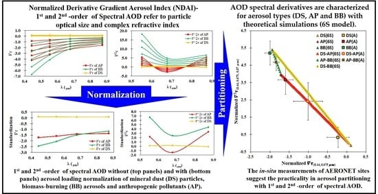
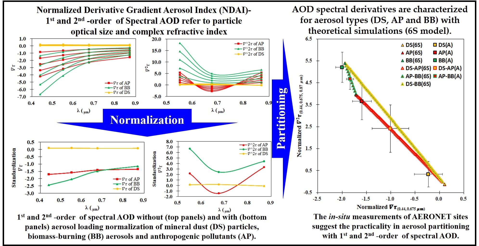
2.2. Spectral Derivatives of AOD

The radiometric differences in the spectral character between aerosols are principally associated with particle size and the imaginary part of the complex refractive index ([51] and references therein). The spectral derivative of optical properties can be further linked to the characteristics of suspended particles in scattering and absorption processes. Regarding spectral characteristics, the optical properties of aerosols are generally wavelength-dependent; for instance, the SSA of DS aerosols increases as the wavelength increases, while those of AP and BB aerosols decrease. Discrepancies in spectral behavior associated with SSA magnitudes can be used as a proxy for discriminating the presented aerosol types [33,36,54]. However, the large-scale identification of aerosol types by means of SSA properties becomes challenging due to insufficient satellite retrievals. Furthermore, regions of mixed aerosols present another constraint for the application of satellite data. On the contrary, the dissimilarities of the spectral AOD between aerosol types indicate the discriminatory potential of AOD gradients; in particular, between BB and AP aerosols. The related studies of the spectral derivative analysis of solar spectroradiometric measurements have also illustrated the differences of radiometric properties in derivative spectra ([51,53] and references therein).

Referencing the Ångström empirical formula [64], the first-order derivative of AOD (∇τ) between the λ₁ and λ₂ interval can be computed as shown in Equation (1) [53],

$$\frac{\partial \tau }{\partial \lambda }\approx \nabla {\tau }_{({\lambda }_1,{\lambda }_2)}=\frac{{\tau }_{{\lambda }_1}-{\tau }_{{\lambda }_2}}{\Delta \lambda }={\tau }_{{\lambda }_2}\times (1-A^{\alpha })\times B,$$

(1)

where $\Delta \lambda ={\lambda }_2-{\lambda }_1$, $A={\lambda }_2/{\lambda }_1$ and $B=1/({\lambda }_2-{\lambda }_1)$ are the constants for the specific spectral bands. λ is the wavelength (μm) and α is the AE (Ångström exponent, related to particle size distribution). Equation (1) shows that the first-order derivative ($\nabla {\tau }_{({\lambda }_1,{\lambda }_2)}$) is a function of particle size distribution (α variable) and aerosol loading (AOD, which is not an intrinsic property of aerosols). Thus, the value of the first-order derivative will vary with aerosol loading, even for the same type. To eliminate the effect of aerosol loadings on the characteristics of the intrinsic property between aerosol types, the spectral derivative is normalized by an AOD loading reference (${\tau }_{{\lambda }_{ref}}$), as shown in Equation (2).

$${\mathrm{NDAI}}_{({\lambda }_1,{\lambda }_2)}\equiv \nabla {\tau }_{({\lambda }_1,{\lambda }_2)}/{\tau }_{{\lambda }_{ref}},$$

(2)

where ${\tau }_{{\lambda }_{ref}}$ can be selected from either ${\tau }_{{\lambda }_1}$, ${\tau }_{{\lambda }_2}$ or another relevant parameter (${\tau }_{{\lambda }_3}$) to bind the dynamic range to the spectral derivative of each type. More importantly, this normalized first-order derivative (named the Normalized Derivative Aerosol Index, NDAI, as defined in Equation (2)) is the most significant intrinsic property for partitioning the AOD fractions (fAOD) of major components in mixed aerosols (see also Section 2.3). Throughout this study, the AOD at the blue band (0.44μm), AOD_(0.44μm), was selected as the normalization reference of aerosol loading (i.e., ${\tau }_{{\lambda }_{ref}}$) for each type. In addition, since the remote sensing and retrievals are ill-posed problems [65], multiple solutions may be involved in the close range of ${\mathrm{NDAI}}_{({\lambda }_1,{\lambda }_2)}$ values (e.g., similar effective particle sizes but different types of pure and/or mixed type aerosols). Thus, the major components needed to be identified before the determination of the fAOD_(NDAI) within mixtures. In terms of the essential properties of scattering and absorption between aerosol types (DS, AP and BB), the second-order derivative of AOD (≅${\nabla }^2{\tau }_{({\lambda }_1,{\lambda }_2,{\lambda }_3)}$) related to the imaginary part of the refractive index [51] was exploited to help identify the major components of mixtures. The second-order derivative of spectral AOD without and with a referenced AOD (${\tau }_{{\lambda }_{ref}}$) normalization can be expressed as Equations (3) and (4), respectively, by approximating the spectrum interval (i.e., λ₂ − λ₁ ≅ λ₃ − λ₂). The wavelengths at 0.44, 0.675 and 0.87μm are selected for ${\lambda }_1,{\lambda }_2,{\lambda }_3$ in above equations, respectively.

$$\frac{{\partial }^2\tau }{\partial {\lambda }^2}\cong {\nabla }^2{\tau }_{({\lambda }_1,{\lambda }_2,{\lambda }_3)}=\frac{({\tau }_{{\lambda }_1}-2{\tau }_{{\lambda }_2}+{\tau }_{{\lambda }_3})}{({\lambda }_1-{\lambda }_2\left)\right({\lambda }_2-{\lambda }_3)}$$

(3)

$$\frac{{\partial }^2\tau }{\partial {\lambda }^2}/{\tau }_{{\lambda }_{ref}}\cong {\nabla }^2{\tau }_{({\lambda }_1,{\lambda }_2,{\lambda }_3)}/{\tau }_{{\lambda }_{ref}}=\frac{({\tau }_{{\lambda }_1}-2{\tau }_{{\lambda }_2}+{\tau }_{{\lambda }_3})/{\tau }_{{\lambda }_{ref}}}{({\lambda }_1-{\lambda }_2\left)\right({\lambda }_2-{\lambda }_3)},$$

(4)

2.3. AOD Partitioning in Aerosol Mixtures

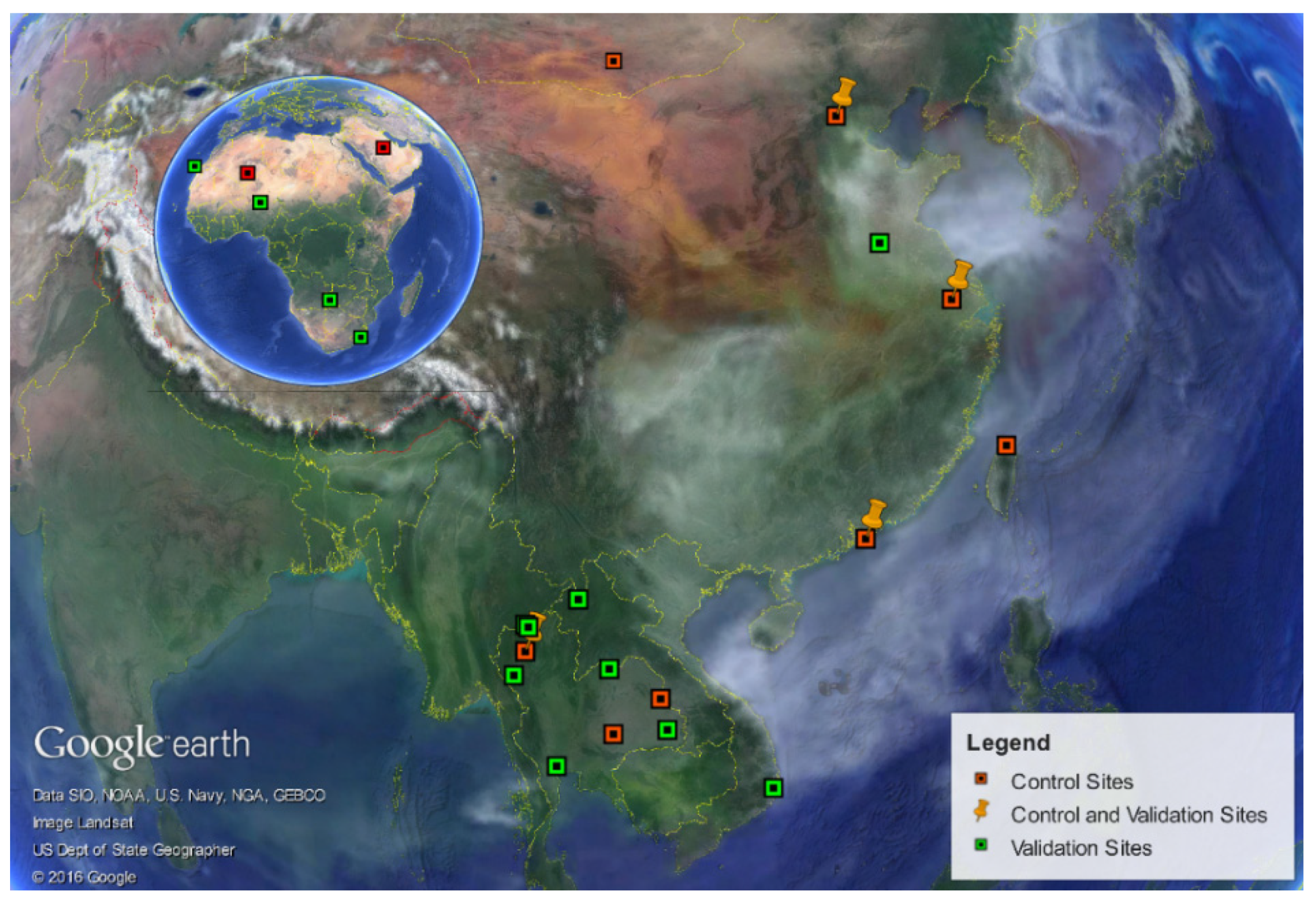
For a dual-type mixture with major components of type A and type B, the change of AOD ($\Delta {\tau }_{({\lambda }_1,{\lambda }_2)}^{ABmixed}$) depends on the AOD fraction (fAOD) of each component, which is described as

$$\Delta {\tau }_{({\lambda }_1,{\lambda }_2)}^{ABmixed}=f_{AOD}^A\Delta {\tau }_{({\lambda }_1,{\lambda }_2)}^A+f_{AOD}^B\Delta {\tau }_{({\lambda }_1,{\lambda }_2)}^B,$$

(5)

where $f_{AOD}^A$ and $f_{AOD}^B$ represent the fAOD_(NDAI) in spectra (${\lambda }_1,{\lambda }_2$) of type A and B aerosols of the mixture, and $f_{AOD}^A+f_{AOD}^B=1$. Based on Equation (2), Equation (5) can be further derived in terms of NDAI as Equation (6).

$${\mathrm{NDAI}}_{({\lambda }_1,{\lambda }_2)}^{ABmixed}=\nabla {\tau }_{({\lambda }_1,{\lambda }_2)}^{ABmixed}/{\tau }_{ref}=f_{AOD}^A{\mathrm{NDAI}}_{({\lambda }_1,{\lambda }_2)}^A+f_{AOD}^B{\mathrm{NDAI}}_{({\lambda }_1,{\lambda }_2)}^B$$

(6)

Equation (6) shows that the ${\mathrm{NDAI}}_{({\lambda }_1,{\lambda }_2)}$ value of a dual-type mixture is a linear composition of NDAI with the AOD fraction of each component, indicating the potential of ${\mathrm{NDAI}}_{({\lambda }_1,{\lambda }_2)}$ in determining the fAOD_(NDAI) of aerosol mixtures. Associated with the intrinsic NDAI property of each type, the fAOD_(NDAI) of dual-type aerosols can be obtained as follows:

$$f_{AO{D}_{}}^A=\frac{\mathrm{NDA}{\mathrm{I}}_{({\lambda }_1,{\lambda }_2)}^{mean-A}-{\mathrm{NDAI}}_{({\lambda }_1,{\lambda }_2)}^{ABmixed}}{{\mathrm{NDAI}}_{({\lambda }_1,{\lambda }_2)}^{mean-A}-{\mathrm{NDAI}}_{({\lambda }_1,{\lambda }_2)}^{mean-B}}$$

(7)

where ${\mathrm{NDAI}}_{({\lambda }_1,{\lambda }_2)}^{mean-A}$ and ${\mathrm{NDAI}}_{({\lambda }_1,{\lambda }_2)}^{mean-B}$ are the intrinsic ${\mathrm{NDAI}}_{({\lambda }_1,{\lambda }_2)}$ values of aerosol type A and type B, while ${\mathrm{NDAI}}_{({\lambda }_1,{\lambda }_2)}^{ABmixed}$ is the ${\mathrm{NDAI}}_{({\lambda }_1,{\lambda }_2)}$ value of type A–B mixtures (see also Figure S1). A similar algorithm for the spectral derivative has been constructed for partitioning relative contributions of aerosols and clouds in spectral fluxes by Hansell et al. [53].

3. Measurements

Using unified, well-maintained and calibrated ground-based sun photometers, AERONET [19] is a globally distributed aerosol observation network whose retrieved aerosol properties have become benchmark references for validating various satellite aerosol retrievals. In this study, all available Level 1.5 and Level 2.0 cloud screened data from 24 stations (Figure 1) during the period from 1997 to 2016 were collected. The spectral AOD and SSA at the wavelengths of 0.44, 0.675, 0.87 and 1.02μm were used to distinguish the optical characteristics for aerosol types. The aerosol particle size distribution (α in Equation (1)) was computed from AODs at the wavelengths of 0.44 µm and 0.675 µm for further analysis in this study. Primary considerations for the AERONET sites selected in this study included (1) the source regions of aerosol emission for DS, BB and AP types, (2) the temporal completeness of data during the study periods and (3) the prior investigations related to aerosol types from AERONET measurements. Figure 1 shows the locations of the selected AERONET sites associated with simulations of AP plumes over East Asia, DS plumes around Central Asia and AP–BB mixed plumes in Southeast Asia.

The in-situ measurements from AERONET sites used in this study include the source regions of DS, AP and BB emissions. The sites of Tamanrasset and the Solar Village stations are located in the DS storm region of Northern Africa and Middle East and were selected for the analysis of DS particles during the wet season (April–September) [8,33,35]. Beijing is located in northwestern China and is on the frequent path of DS plumes transported from the Takalamkan and Gobi deserts to eastern Asia. Accordingly, the measurement from Beijing station provides a unique chance to better understand the optical properties of DS aerosols in Asia. Therefore, observations from Beijing, Solar Village and Tamanrasset stations were used as the reference of DS aerosol properties. Since urban and industrial areas are generally the source regions of AP emission, references of AP aerosols were collected from the stations located in urban areas (e.g., Taihu, Taipei, Beijing and Hong Kong) during air pollution episodes. To exclude the influence of DS or BB aerosols in Asia, the observations were only collected in August and September for AP properties. BB events occur frequently in Indochina and southeast China during springtime and summertime, respectively. During these seasons, the deliberate burning of forest, crops and rice bran to reclaim agricultural land produces large amounts of BB aerosols [66,67,68,69]. The AERONET in Pimai, Mukdahan, Chiang Mai was thus selected as the source region of BB optical properties. The data listed in

Table 2. The control dataset and validation dataset from source regions of AERONET sites for aerosol type identification during the periods from 1997 to 2012 and 2014 to 2016, respectively. NDAI: normalized difference aerosol index.

Control dataset (for NDAI approach construction).
DS	BB	AP
April–May	March–May	August–September
Beijing (39N,116E) 2001–2012	Chiang Mai (18N,98E) 2006–2012	Beijing (39N,116E) 2001–2012
Dalanzadgad (43N,104E) 1997–2012	Mukdahan (16N,104E) 2003–2010	Hong Kong (22N,114E) 2005–2012
Solar Village (24N,46E) 1998–2012	Pimai (15N,102E) 2003–2008	Taihu (31N,120E) 2005–2012
Tamanrasset (22N,5E) 2006–2012		Taipei (25N,121E) 2002–2012
Validation dataset (for NDAI product validation)
DS	BB	AP
April–May(2014–2016)	March–May(2014–2016)	August–September(2014–2016)
Beijing (39N,116E)	Chiang Mai (18N,98E)	Beijing (39N,116E)
La Laguna (28N,16W)	Doi Ang Khang (19N,99E)	Durban UKZN (30S, 31 E)
XuZhou (34N,117E)	Luang Namtha (20N,101E)	Hong Kong (22N,114E)
Zinder Airport (14N, 9E)	Maeson (19N,99E)	La Laguna (28N,16W)
	Mongu Inn (15S, 23E)	Mongu Inn (15S, 23E)
	NhaTrang (12N,109E)	Taihu (31N,120E)
	Omkoi (17N,98E)	Taipei (25N,121E)
	Silpakorn Univ (13N,100E)	XuZhou (34N,117E)
	Ubon Ratchathani (15N,104E)
	Vientiane (17N,102E)

were collected under manual supervision from each AERONET site with an AOD larger than 0.4 for the control dataset and validation dataset, respectively. The optical properties of each type (DS, BB and AP) were characterized based on the control dataset for the NDAI approach, while the validation dataset was employed to evaluate the performance of the NDAI approach.

4. Results and Analysis

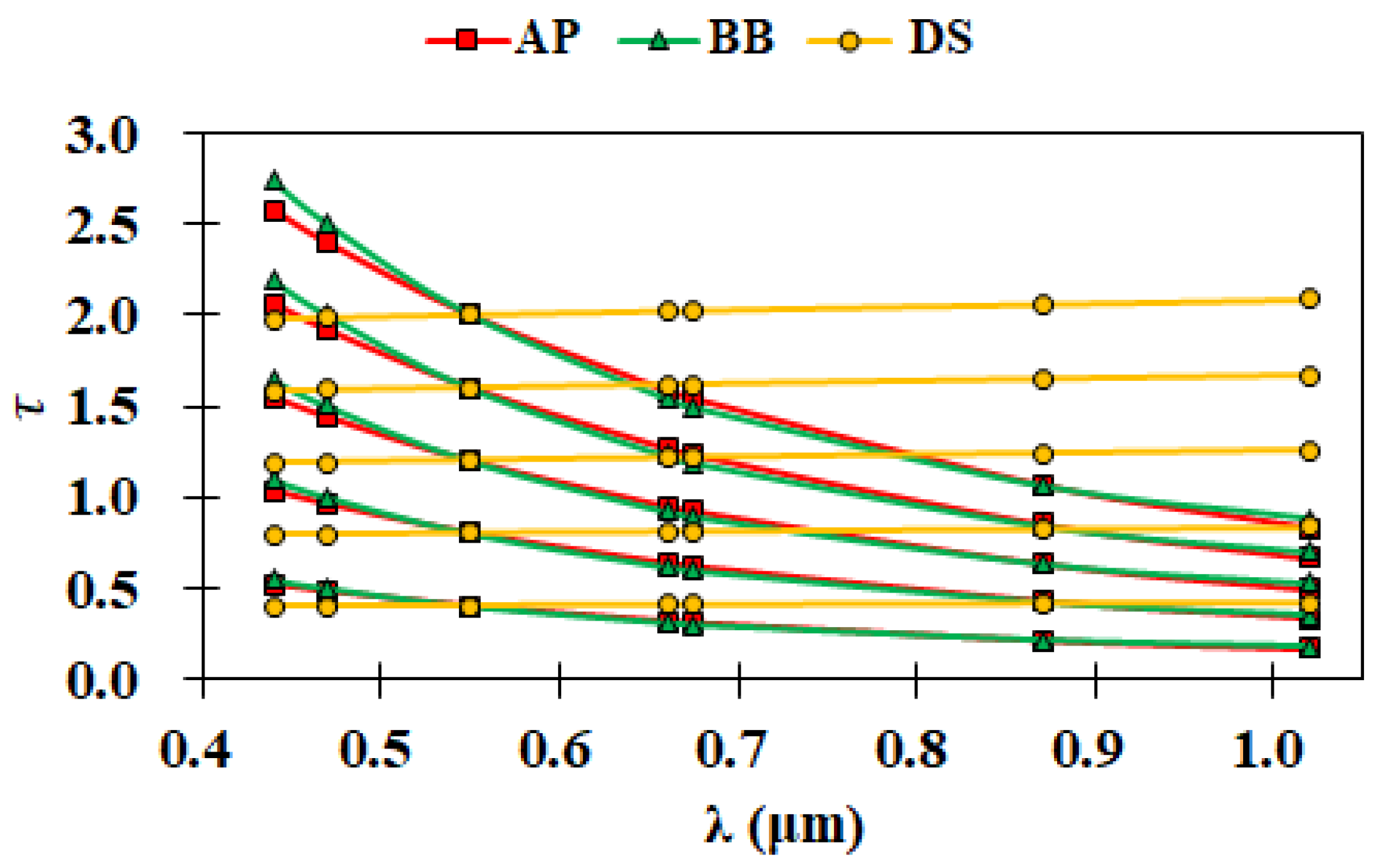
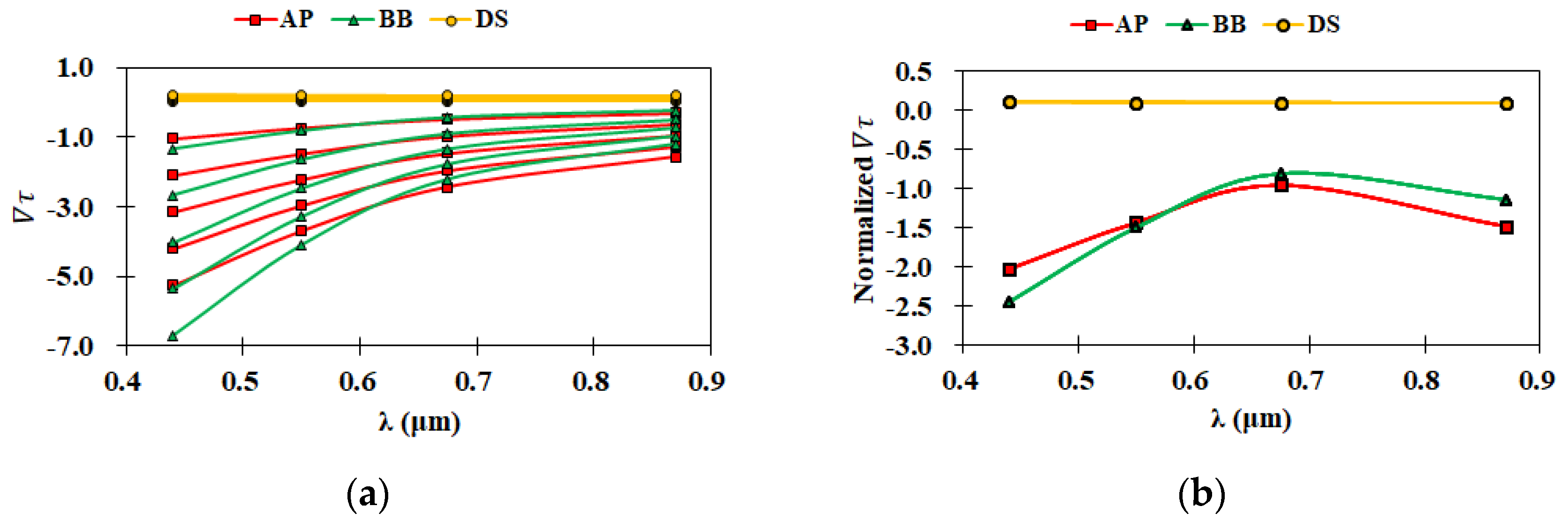
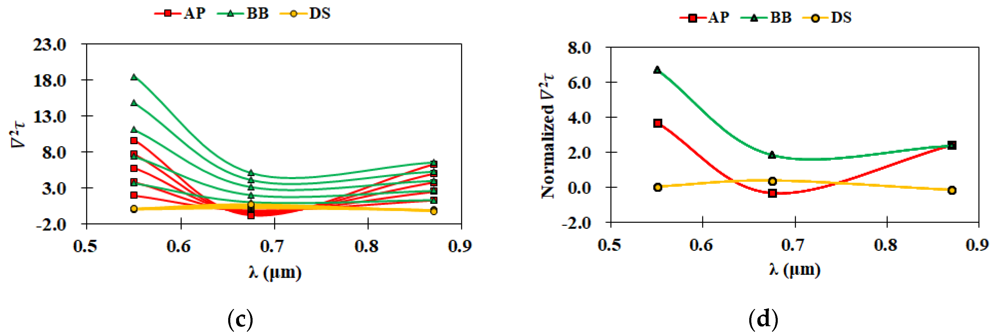
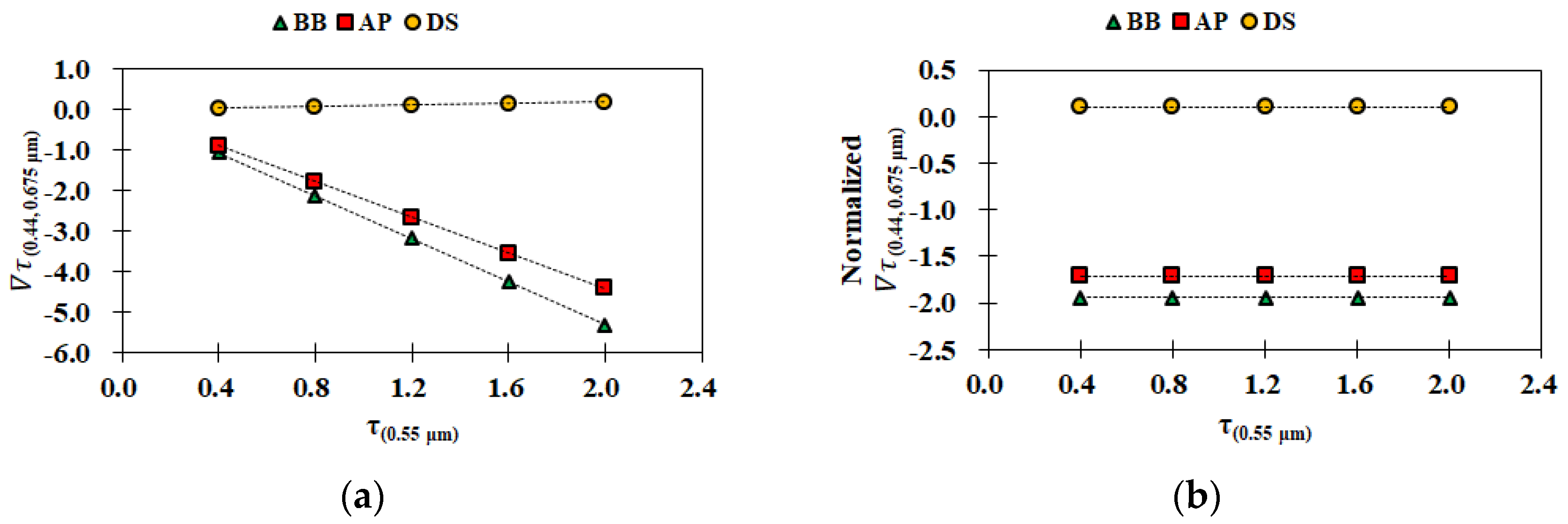
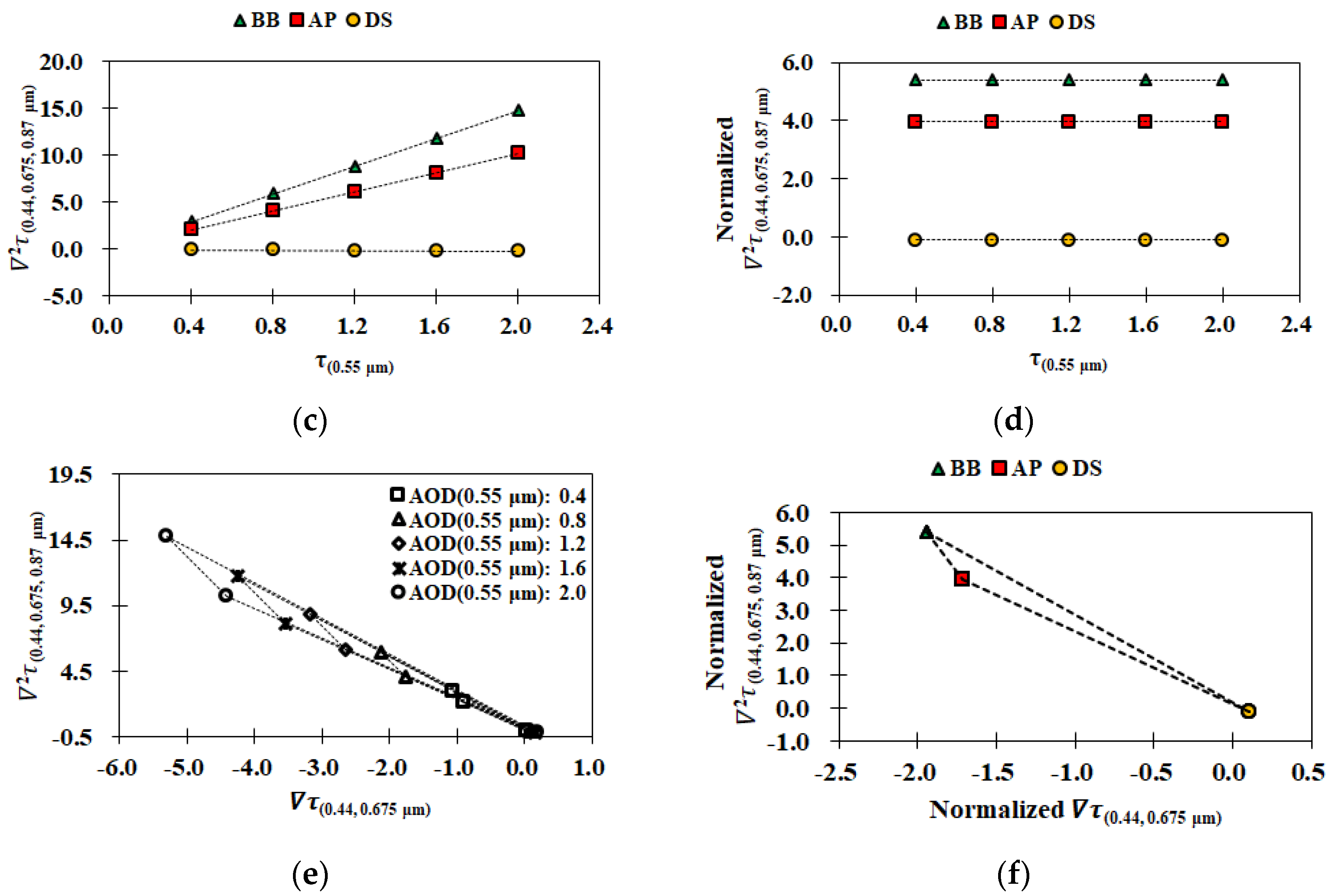
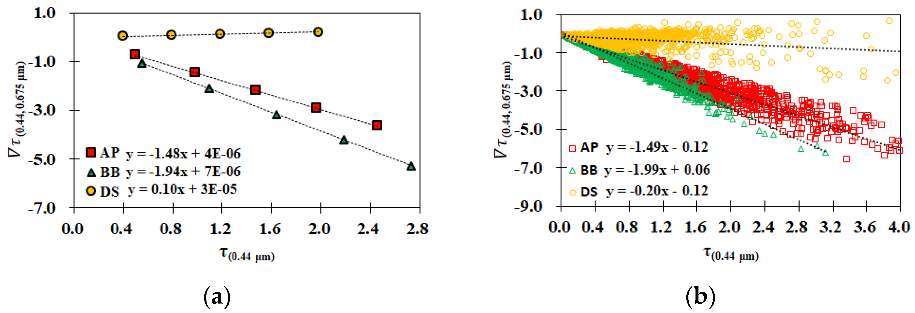
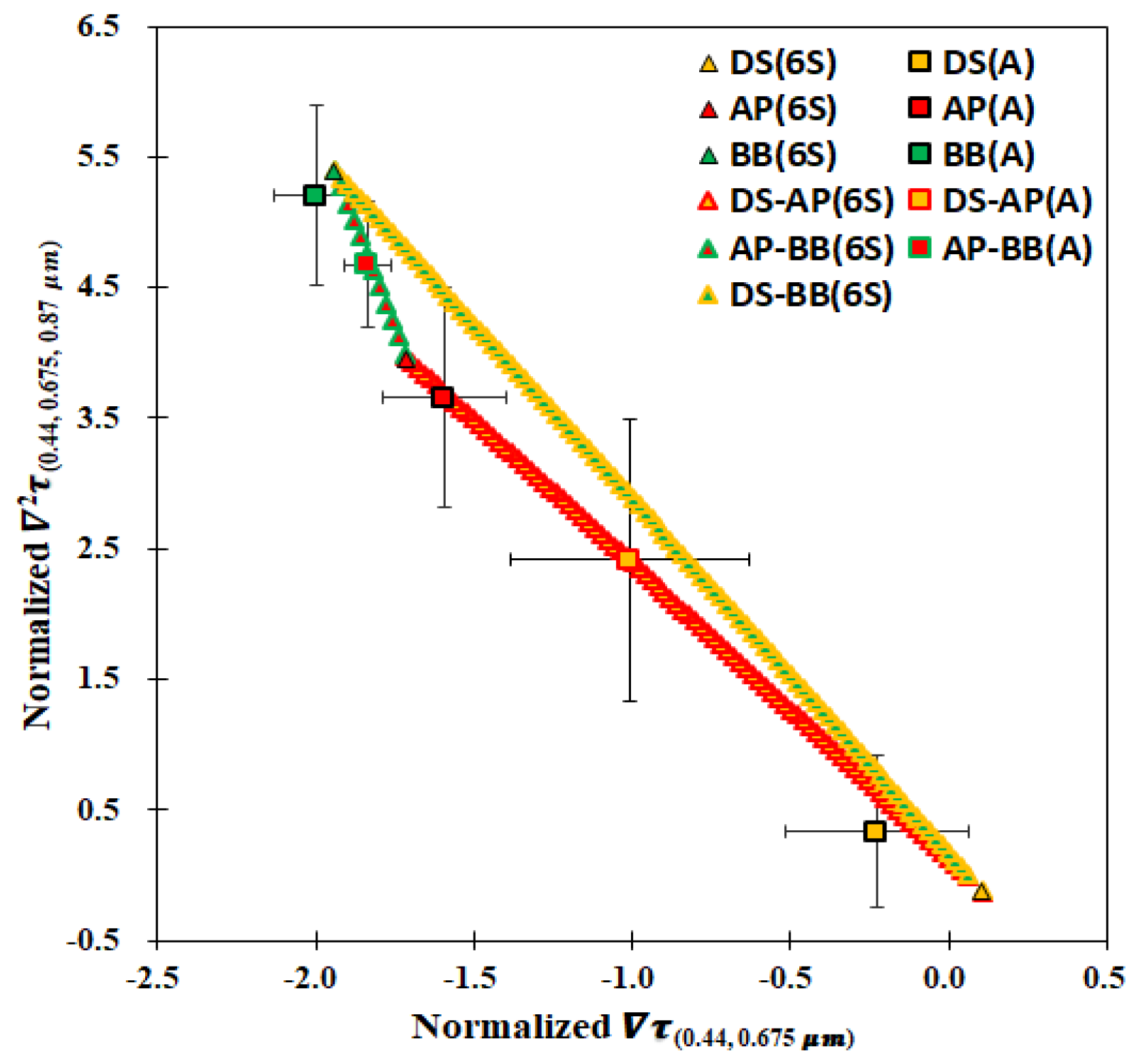
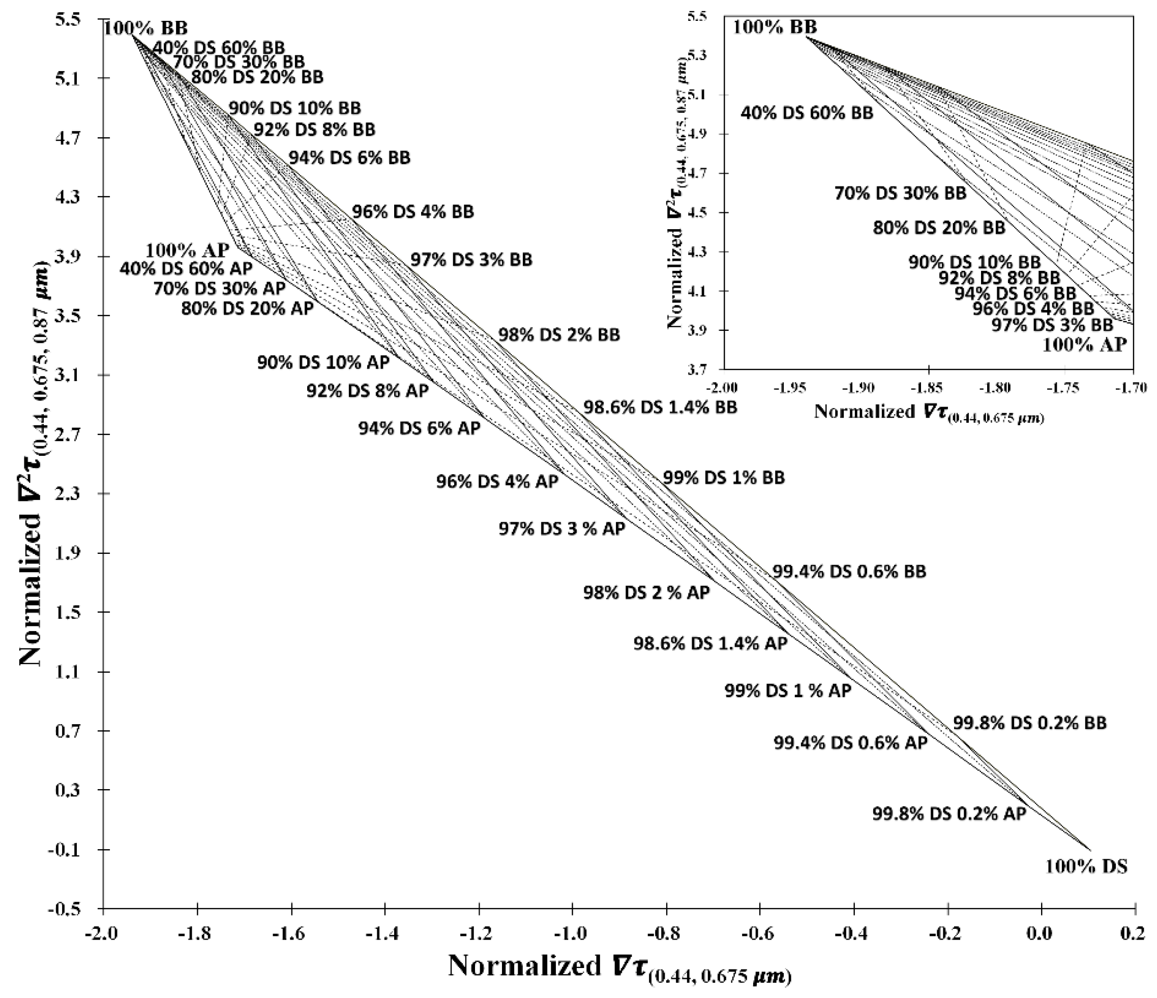
4.1. Theoretical Spectral AOD Derivatives

The spectral distributions of AOD at specific wavelengths (0.44, 0.47, 0.55, 0.66, 0.675, 0.87 and 1.02 μm) for various aerosol loadings were simulated from 6S with the experimental dataset (Table 1) for each aerosol type and are presented in Figure 2. Applying the Bezier curve method, the discrete points were connected. The spectral distribution of DS particles (yellow lines) revealed a flat trend with small increases correlated with wavelength, while AP and BB aerosols (red and green lines) tended to decrease constantly, which were similar results to previous studies [56,70]. As the Ångström exponent showed, the spectral gradient was primarily related to the particle size information, indicating that the radius of DS particles was much greater than the counterparts of AP and BBs. Although a similar particle size may have raised the difficulty in discriminating AP from BB, their spectral gradients were still slightly different. In addition, it is worthy of notice that the gradient of spectral AOD could vary with aerosol loading (AOD_(0.55µm) value of 0.4, 0.8, 1.2, 1.6 and 2.0) even for the same type.

Detailed changes in simulated spectral AODs can be difficult to discern between AP and BB particles in a zeroth-order spectrum, as shown in Figure 2. However, spectral derivatives can facilitate the identification of subtle changes in AOD resulting from different scattering and absorption processes. Thus, spectral derivatives could be a potential link to particle size and complex refractive indexes to enhance the intrinsic characters of particles, as also suggested by Hansell et al. [51]. Based on the data shown in Figure 2, Figure 3a depicts the first-order derivative of AOD,$\nabla {\tau }_{({\lambda }_1,{\lambda }_2)}$, derived from the spectral pairs of 0.44–0.55, 0.55–0.675, 0.675–0.87 and 0.87–1.02 (μm) for DS, AP and BB aerosols, respectively. Different curves in the same color stand for the AOD_(0.55µm) values of 0.4, 0.8, 1.2, 1.6 and 2.0 respectively. The values of $\nabla {\tau }_{({\lambda }_1,{\lambda }_2)}$ for DS aerosols became almost flat (i.e., they all tended to zero) with wavelength. It is obvious that the gaps in $\nabla {\tau }_{({\lambda }_1,{\lambda }_2)}$ between AP and BB aerosols altering and deviating with aerosol loading become more pronounced in shorter wavelength spectra except for DS (due to the flat distribution of spectral AOD). For the second-order derivative of AOD before loading normalization, three sets of DS, AP and BB aerosols each with three sequential spectral AODs (0.44–0.55–0.675, 0.55–0.675–0.87 and 0.675–0.87–1.02 μm) are examined, as shown in Figure 3b. Although the difference between AP and BB aerosols can be more enlarged in terms of ∇²τ, the value of the second-order derivative is still loading-dependent, in a similar manner to the situation of $\nabla {\tau }_{({\lambda }_1,{\lambda }_2)}$, as shown in Figure 3a. Both first and second-order derivatives indicated the importance of normalization if an intrinsic character is required. After normalizing with the AOD_(0.44μm), as shown in Figure 3c,d, the curves of each type in different loadings began to merge together into their own intrinsic spectrums. The loading effect was efficiently eliminated in the intrinsic values of DS, AP and BB aerosols.

Visible bands are most sensitive to atmospheric aerosols, which could result in significant differences in spectral derivatives. However, it is not clear how to identify the aerosol types with the values of first and second-order derivatives ($\nabla {\tau }_{(0.44,0.675)}$ and ${\nabla }^2{\tau }_{(0.44,0.675,0.87)}$) in the conditions of slight aerosol loading, as illustrated in Figure 4a,c. On the contrary, the intrinsic characteristics of each aerosol type from normalized derivatives are shown to be independent to the loading effect (Figure 4b,d). The constant value even with obviously dissimilar intrinsic derivatives between types facilitates the identification of aerosol types with more confidence.

Table 3. The optical properties of AP, BB and DS aerosols from AERONET measurements and 6S simulations from the experimental dataset. The AERONET dataset is screened with an AOD_(0.44μm) of more than 0.8 with the single-scattering albedo (SSA)_(0.675μm) criterion. AE: Ångström exponents.

Data Source	Aerosol Intrinsic Property	DS (n = 205)	AP (n = 394)	BB (n = 85)
Instrument observation (AERONET)	AOD(0.44μm)	1.24 ± 0.55	1.47 ± 0.66	1.33 ± 0.38
	AE(0.44, 0.675μm)	0.25 ± 0.21	1.12 ± 0.16	1.54 ± 0.12
	SSA(0.675μm)	0.95 ± 0.01	0.93 ± 0.01	0.89 ± 0.01
	NDAI(0.44, 0.675, τ(ref)=0.44μm)	−0.27 ± 0.26	−1.62 ± 0.18	−2.05 ± 0.11
	NDAI(0.44, 0.675, τ(ref) = 0.675μm)	−0.31 ± 0.32	−2.65 ± 0.46	−3.98 ± 0.43
	NDAI(0.44, 0.675, τ(ref)=0.87μm)	−0.33 ± 0.34	−3.73 ± 0.80	−6.22 ± 0.75
	NDAI(0.44, 0.675, τ(ref)=1.02μm)	−0.35 ± 0.36	−4.71 ± 1.14	−8.60 ± 1.34
Theoretical simulation (6S model and experiment dataset)	AOD(0.44μm)	1.19 ± 0.40	1.48 ± 0.49	1.64 ± 0.55
	AE(0.44, 0.675μm)	0.16	1.05	1.50
	SSA(0.675μm)	0.95	0.95	0.87
	NDAI(0.44, 0.675, τ(ref)=0.44μm)	−0.28	−1.58	−2.07
	NDAI(0.44, 0.675, τ(ref)=0.675μm)	−0.30	−2.81	−4.39
	NDAI(0.44, 0.675, τ(ref)=0.87μm)	−0.30	−3.86	−6.19
	NDAI(0.44, 0.675, τ(ref)=1.02μm)	−0.30	−4.84	−7.48

summarizes the optical properties for DS, AP and BB aerosols based on 6S simulations. However, most of the cases we faced were not merely of the pure type; the optical properties usually diversified after the types mixed. The application of intrinsic properties from the pure type was therefore limited. Thus, the dynamic ranges caused by the mixing effect between DS, AP and BB were explored in terms of first and second-order derivatives. The discrepancy of intrinsic values between each pure type was recognizable in the domain of spectral derivatives, as shown by the symbols located in Figure 4e,f. It was obvious that the spectral derivatives of AP and BB varied with aerosol loading (Figure 4e) but converged after normalization (Figure 4f). The chained lines between symbols, respectively, indicate the dynamic ranges of DS–AP, DS–BB and AP–BB mixtures and demonstrate the weighting potentials among the major components.

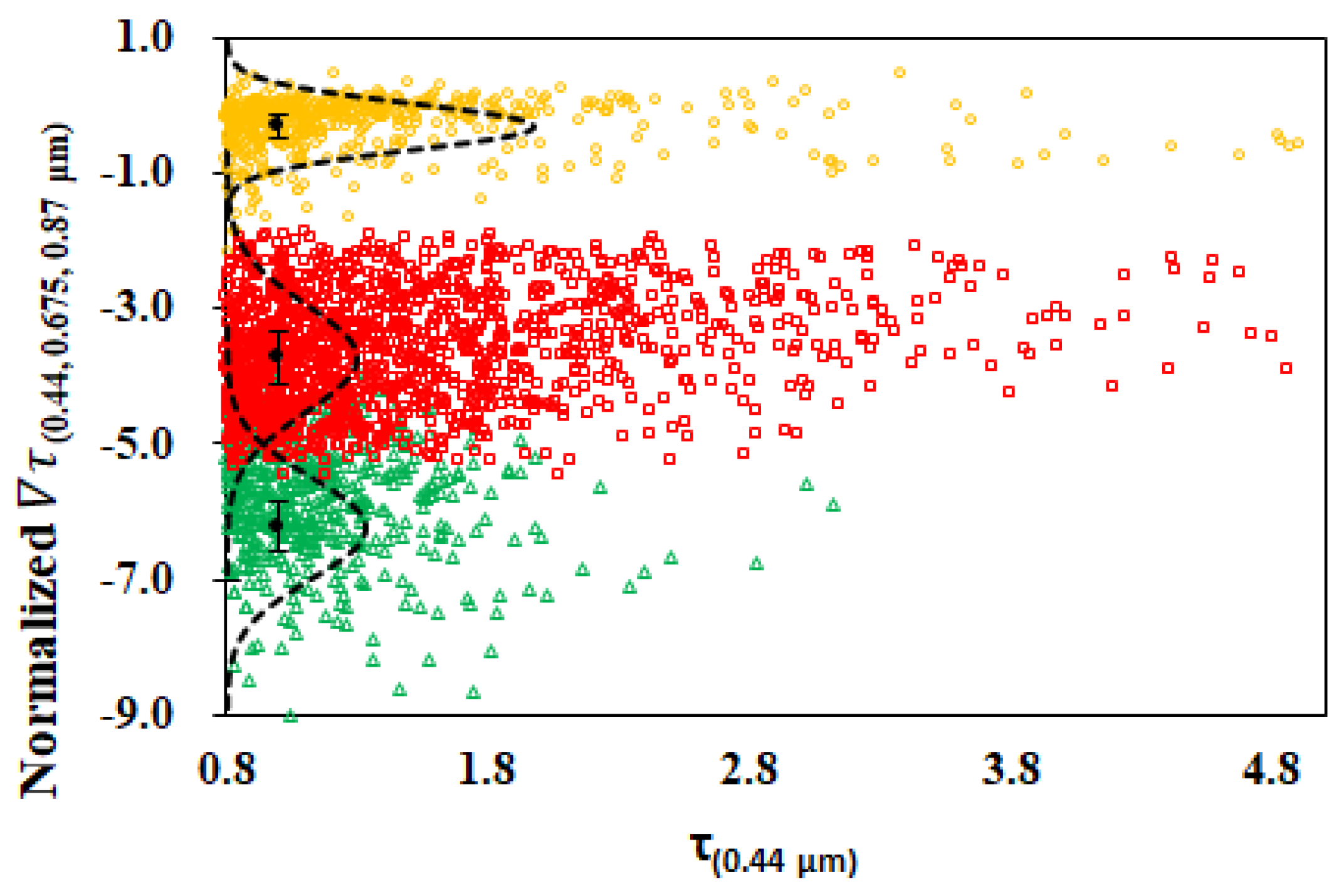
4.2. Measurements for Spectral AOD Derivatives

To ensure data quality, the measurements were generally checked with and AOD_(0.44μm) larger than 0.8 for further applications [33,54,71]. In this study, the severer criteria (AOD_(0.44μm) > 0.8) with confident parameters (e.g., SSA) were considered for preferable data filtering. As a result, a total of 684 AERONET data points were selected (i.e., the control dataset in Table 2) for the optical characteristics of each aerosol type that dominated in source regions. The optical properties exhibited by each type are summarized in Table 3, including AOD_(0.55μm), AE_{(0.44, 0.675μm)}, SSA_(0.675μm) as well as NDAI. The AOD values of different aerosol types (DS, BB and AP) indicated a kind of concentration loading of aerosols emitted around the selected source regions. Since the value of AE_DS differed from the others (AE_BB and AE_AP), the AE value was utilized to distinguish between DS and non-DS aerosols over land.

In comparison with in-situ measurements, the simulated 6S spectral distributions of AODs were appropriate, especially the patterns of AP and BB aerosols. Since in-situ measurements of pure DS aerosols are extremely rare, the simulated AE value (0.16) of DS was reasonably different from that of AERONET (0.25). Owing to the strong absorption, the SSA of BB aerosols was significantly smaller than DS and AP aerosols. The values of SSA_DS (0.95 ± 0.01), SSA_BB (0.89 ± 0.01) and SSA_AP (0.93 ± 0.01) in Table 3 were consistent with previous studies [31,72,73,74,75,76]. The derived values of AOD_(0.55µm), AE_{(0.44, 0.675μm)} and NDAIs were also consistent with AERONET measurements. Furthermore, the discrepancies of DS, AP and BB aerosols in NDAI_{(0.44, 0.675, 0.44μm)} values between AERONET and the 6S model (theoretical simulations) were 4%, 2% and 1%, respectively, supporting the proposed NDAI approach, with high potential for aerosol type discrimination and also confirming the appropriateness of site selection for dominant aerosol types.

As the first-order derivative of spectral AODs(_{(0.44, 0.675)}) demonstrates, both model simulations (Figure 5a) and AERONET measurements (Figure 5b) revealed the variabilities in particle size (α) and aerosol loading (τ). Moreover, the slope of each aerosol type from theoretical simulations was even more consistent with the in-situ measurements, strongly supporting the proposed NDAI approach in this study. However, the gradients of AP and BB groups were apparently overlaid when the aerosol loading became small, even AOD value higher than 1.0 as Figure 5b shows, which would cause confusion in aerosol type identification.

After normalization with aerosol loading using the NDAI, as defined by Equation (2), the dynamic range of the first-order derivatives of spectral AODs for each aerosol type was clearly separated. Generally, the performance of normalization with different spectra is similar after examinations (see Figure S2 for results using four spectral AOD normalizations). While, in Figure 6, the first-order derivative normalized with AOD_(0.87μm) was selected from Figure S2 since its normal distribution mapping was relatively better than other reference wavelengths. The results largely conformed to the theoretical simulations (Figure 4b). For the case normalized by the aerosol loading of _(0.87μm), the NDAI values of DS, AP and BB aerosols ranged within −0.33 ± 0.34, −3.73 ± 0.80 and −6.22 ± 0.75, respectively, facilitating the discrimination of aerosol types. The results also indicated that the particle size distribution of BB aerosols could be discriminated from the counterparts of AP aerosols after AOD normalization. It is worth noting that the intrinsic properties were generally independent of loading (i.e., AOD), implying the results after normalization are also available to the cases of AOD smaller than 0.8. The intervals of the normalized ∇τ (NDAI values) outside the dynamic ranges of pure aerosol types were initially considered to correspond to the situations of mixed types or other aerosols, known as the overlapping regions in the first-order derivative of spectral AODs, such as the intervals between DS–AP, AP–BB and DS–BB. The NDAI within the DS–BB interval may be confused with the overlap of DS–AP mixtures. Thus, the major components of mixtures should be identified before fAOD partitioning.

Based on the discrepancy of each aerosol type in scattering and absorption (i.e., refractive index), the second-order derivative of the spectral AOD (∇²τ) is explored to identify the major components of mixtures. Firstly, the second-order derivative (normalized ∇²τ) versus the first-order derivative (normalized ∇τ) simulated from the 6S model was examined with a fine level (0.01) of mixing weight of volume density for the mixtures with two major components. The relationship between first and second-order spectral derivatives basically followed a quadratic polynomial along with the mixing weight of components, but it also could be well described by the linear relationship within 0.44–0.87 µm spectra, as Figure 7 shows. Theoretically, the curves of these relationships could be considered as the boundary of dual-type mixtures (i.e., DS–AP, DS–BB and AP–BB) in the spectral derivative domain, and the locations inside the triangle region composed by these curves were mixtures between the three major types presented (see also Figure 10 in Section 5). The results exhibited that the mean value of DS–BB in the value of the normalized ∇²τ was much higher than the value of DS–AP mixtures. Furthermore, the overlapping interval in the first-order derivative (normalized ∇τ) among DS–BB mixtures and AP aerosols, as Figure 6 shows, can be properly discerned as well. The first and second-order spectral derivatives of DS, AP, BB, DS–AP, DS–BB and AP–BB aerosols from in-situ measurements of AERONET sites also suggested the practicality in aerosol partitioning, as shown in Figure 7. Therefore, the normalized first-order derivative (known as NDAI value) associated with the second-order derivative was eventually found for aerosol partition in pure type and major components, including DS, AP, BB, DS–AP, DS–BB and AP–BB species in this study. It is important to emphasize the capability of discriminating AP from BB aerosols in the spectral derivative domain, even for the mixtures. Associated with the intrinsic spectral derivatives of major components (Table 3), the AOD fractions of mixtures can be further partitioned according to the NDAI value (normalized ∇τ) of the mixture.

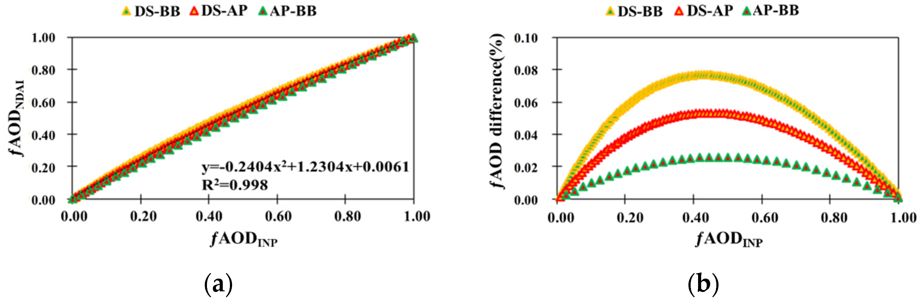
4.3. Verification of AOD Fraction from NDAI

After the major components of mixtures could be potentially identified, two datasets were used to examine the usefulness of the NDAI approach for AOD fractions, named “fAOD_NDAI” and “fAOD_INP”. The AOD fractions partitioned by the proposed NDAI approach according to the simulated spectral AOD are denoted as the fAOD_NDAI dataset, while the AOD fractions (fAOD_INP) derived from inputs of mixing weights were taken as the reference of fAOD_NDAI evaluation (see also Section 2.3). The results of all dual-component mixtures demonstrated high consistency (R² = 0.998) between fAOD_NDAI and fAOD_INP, as Figure 8a shows. The differences of AOD fraction determined by NDAI approach (fAOD_NDAI) from initial inputs (fAOD_INP) are less than 0.08% after detailed comparison as shown in Figure 8b. The maximum discrepancies occurred at the fractioned value of 0.5 and were principally caused by the linear assumption in fAOD determination from a quadratic polynomial distribution alike, as shown in Figure 8a. Furthermore, the particle size could be the other factor leading to larger uncertainty (e.g., DS–AP and DS–BB in Figure 8b) due to the NDAI being defined as a function of particle size distribution (e.g., α value). For instance, a larger DS particle may result in more fluctuation than the smaller particles (AP and BB), demonstrating the size effect according to Mie scattering theory. The overall results, nevertheless, still exhibit the capability of the NDAI approach in partitioning aerosols.

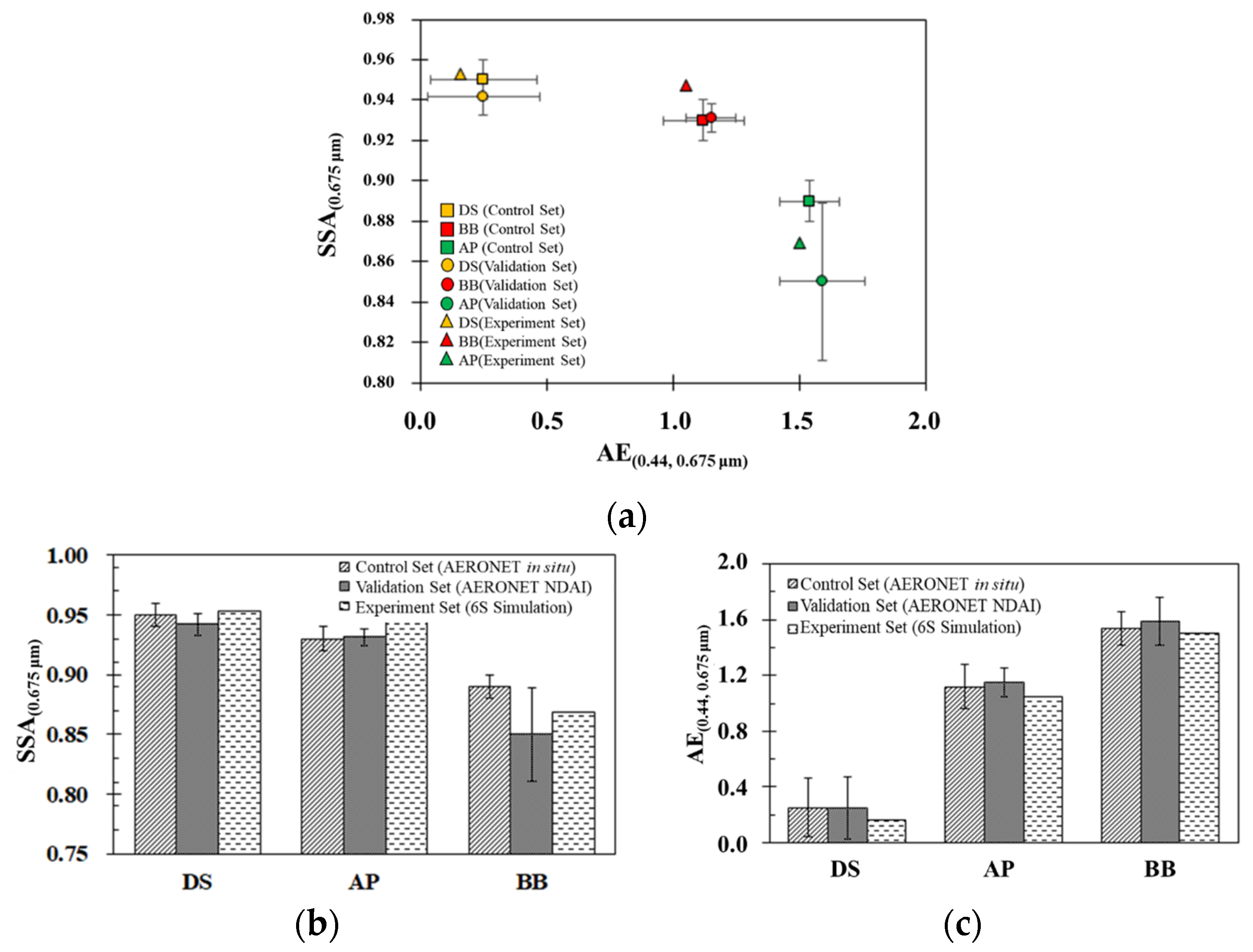
4.4. Validation of Aerosol Type with In-Situ Measurement

In Southeast and Eastern Asia, the seasons of March–May, April–May and August–September are favorable to the emission of BB, DS and AP aerosols, respectively. As a significant property to distinguish different clusters of aerosols, the SSA and AE parameters were used to validate and confirm whether the NDAI method contained information of aerosol absorption. For aerosol type identification and validation by the NDAI approach, in-situ measurements of 18 AERONET sites principally located nearby the source regions (cf. Figure 1) were examined according to the validation dataset in Table 2. A total of 190-point measurements with heavy loading (AOD > 0.8) corresponding with AERONET data from 2014 to 2016 were selected manually for the examination of the NDAI approach to aerosol type identification.

Corresponding to the in-situ measurements of AERONET, Figure 9a depicts the SSA_(0.675μm) and AE_{(0.44, 0.675μm)} mean value of each type (DS,AP and BB) of aerosol based on NDAI categorization from the validation dataset (from 2014 to 2016) and experiment dataset of the 6S model in comparison with the counterparts of the control dataset (from 1997 to 2012). The overall SSA_(0.675μm) and AE_{(0.44, 0.675μm)} results of aerosol categorization based on the NDAI method exhibit high similarity between 6S model simulations and in-situ measurements of the control dataset, as shown in Figure 9a. The detailed difference between validation (AERONET NDAI) and control (AERONET in situ) datasets in SSA_(0.675μm) were 0.86%, 0.13% and 4.5% for DS, AP and BB, respectively, while the differences between control and experiment datasets in SSA_(0.675μm) were 0.32%, 1.83% and 2.36% for DS, AP and BB, respectively (see Figure 9b). Because more AERONET sites were included in the validation dataset (Table 2), the difference of the by aerosol type in SSA_(0.675μm) between validation and control datasets might be caused from the burning materials related to regional land use/land cover; for example, agricultural wastes and forest fire. Nevertheless, the overall results of SSA_(0.675μm) were similar to the control dataset. The overall AE_{(0.47, 0.66μm)} results of aerosol categorization from AERONET NDAI reveal high similarity between 6S-modeled simulations and in-situ measurements, as Figure 9c illustrates, strongly supporting the high potential for aerosol type discrimination of the NDAI approach.

5. Discussion

With the employment of the current NDAI approach, the fractions of mixed aerosol types that frequently appear over Central Africa, East and Southeast Asia can be potentially partitioned/synthesized in terms of their optical properties. For the application of the NDAI approach in reality, atmospheric aerosols usually include all of the three types (i.e., DS, AP and BB). Indeed, as demonstrated in Figure 10, based on the experimental dataset, the first and second-order derivatives of the spectral AOD may have high potential for the partitioning of triple-type mixtures on the basis of the database constructed with three-model mixtures. In Figure 10, the first-order derivatives (∇τ) are calculated from 0.44 and 0.675 µm for the optical properties of particle size distribution, with steps of 0.01 from 0.00 to 1.00 for the mixture of the weights of the volume density. In contrast, the second-order derivatives (∇²τ) are calculated from 0.44, 0.675 and 0.87 µm for the optical properties related to the refractive index. The results indicate the potential of three-model mixtures partitioning (i.e., DS, AP and BB aerosols). Nevertheless, the extension of this application to cover more real-world cases, the required database with in-situ measurements have to be constructed; in particular, the differences of regional aerosol properties in terms of particle size distribution and the complex index of refraction cannot be neglected.

It is well understood that the first derivative of spectral optical depth (or Angstrom exponent) reveals the size dependence, particularly the normalized one (Figure 3c) in separating the fine-mode (AP and BB) from coarse-mode (DS) aerosols. Furthermore, the second derivative of spectral optical depth, with respective to the normalized one that major contribution of size parameter to the optical depth been suppressed, enhances the subtle influence of refractive index between AP and BB (Figure 3d). These analyses form the basis for constructing the principle of partition shown in Figure 4. Thus, it was not the intension of this study to resolve completely the issues incurred in aerosol retrievals; instead, we demonstrated an effective yet simple method for partitioning aerosol type and loading under current setup and assumptions. It is our intension to continue fine-tuning the method and relaxing assumptions involved.

6. Conclusions and Future Work

Considering the intrinsic characteristics of optical size distribution, spectral absorption and scattering, the spectral derivatives of AOD for partitioning aerosol types among dust (DS), anthropogenic pollutant (AP) and biomass burning (BB) particles in AOD fraction are proposed and demonstrated in this study. Based on the theoretical simulations (6S model) and in situ measurements (AERONET) near source regions, the first and second-order AOD derivatives are shown to be highly sensitive to the aerosol particle size distribution and complex index of refraction (SSA). With the discrepancies of BB, AP and DS aerosols in the derivatives of spectral AODs, an approach—namely the Normalized Derivative Aerosol Index (NDAI)—is introduced to partition the AOD components of mixed aerosol types. The theoretical 6S simulations with the NDAI approach agreed well with in-situ measurements from AERONET (with a discrepancy less than 10%). This investigation also delivers an aerosol index for the discrimination of BB from AP aerosols to circumvent the constraint of insufficient SSA data, which reveals high potential for the application of the approach to satellite observations. In summary, the potential contribution of the NDAI approach could be expected to be as follows: (1) to partition the major components of aerosol types based on their multi-spectral optical depth; (2) to potentially map out the spatial distribution of AOD dominated by DS, BB and AP aerosols by means of satellite observations; and (3) to optimistically compensate for the lack of SSA measurements while assessing aerosol radiative forcing. It is also noted that the concept of approach proposed for aerosol partition could be more significant than its further applications in this study.

However, there are two issues related to the effect of surface reflectivity on AOD retrieval and the spectral characteristics of sea salt aerosols when applying the NDAI approach to satellite observations to partition aerosol types and loadings. The NDAI approach at present is only suitable to applications over land due to the lack of sea salt spectral optical properties over ocean areas. For land areas, the accuracy of spectral AODs retrieved from satellite observation is still affected by the uncertainty of surface reflectivity. Therefore, it is anticipated that the above issues will be addressed for the application of our approach to satellite observations, including the partitioning of tri-component aerosols over land and sea salt species discrimination over oceanic regions in the follow-up research works. Once the satellite observations are available for the partitioning of aerosol types and loadings in quantifying aerosol properties over a regional or global scale, the spatiotemporal variations of aerosol radiative forcing can be reasonably mapped to facilitate the further analysis of global warming and climate changes.

References

1. Myhre, G.; Shindell, D.; Bréon, F.; Collins, W.; Fuglestvedt, J.; Huang, J.; Koch, D.; Lamarque, J.; Lee, D.; Mendoza, B.; et al. Anthropogenic and natural radiative forcing. In Climate Change 2013: The Physical Science Basis. Contribution of Working Group I to the Fifth Assessment Report of the Intergovernmental Panel on Climate Change, 5th ed.; Stocker, T.F., Qin, D., Plattner, G.-K., Tignor, M., Allen, S.K., Boschung, J., Nauels, A., Xia, Y., Bex, V., Midgley, P.M., Eds.; Cambridge University Press: Cambridge, UK; New York, NY, USA, 2013; pp. 659–740. [Google Scholar]
2. Haywood, J.; Shine, K. The effect of anthropogenic sulfate and soot aerosol on the clear sky planetary radiation budget. Geophys. Res. Lett. 1995, 22, 603–606. [Google Scholar] [CrossRef]
3. Feng, N.; Christopher, S.A. Clear sky direct radiative effects of aerosols over Southeast Asia based on satellite observations and radiative transfer calculations. Remote Sens. Environ. 2014, 152, 333–344. [Google Scholar] [CrossRef]
4. Lin, T.-H.; Yang, P.; Yi, B. Effect of black carbon on dust property retrievals from satellite observations. J. Appl. Remote Sens. 2013, 7, 073568. [Google Scholar] [CrossRef] [Green Version]
5. Kahn, R.A.; Gaitley, B.J. An analysis of global aerosol type as retrieved by MISR. J. Geophys. Res. Atmos. 2015, 120, 4248–4281. [Google Scholar] [CrossRef]
6. Chang, K.-E.; Hsiao, T.-C.; Hsu, N.-Y.; Wang, S.-H.; Lin, N.-H.; Liu, G.-R.; Liu, C.; Lin, T. Mixing weight determination for retrieving optical property of polluted dust with MODIS and AERONET data. Environ. Res. Lett. 2016, 11, 085002. [Google Scholar] [CrossRef] [Green Version]
7. Kim, J.; Lee, J.; Lee, H.C.; Higurashi, A.; Takemura, T.; Song, C.H. Consistency of the aerosol type classification from satellite remote sensing during the Atmospheric Brown Cloud–East Asia Regional Experiment campaign. J. Geophys. Res. Atmos. 2007, 112, D22S33. [Google Scholar] [CrossRef]
8. Lee, J.; Kim, J.; Song, C.; Kim, S.; Chun, Y.; Sohn, B.; Holben, B. Characteristics of aerosol types from AERONET sunphotometer measurements. Atmos. Environ. 2010, 44, 3110–3117. [Google Scholar] [CrossRef]
9. Eck, T.F.; Holben, B.N.; Sinyuk, A.; Pinker, R.T.; Goloub, P.; Chen, H.; Chatenet, B.; Li, Z.; Singh, R.P.; Tripathi, S.N.; et al. Climatological aspects of the optical properties of fine/coarse mode aerosol mixtures. J. Geophys. Res. 2010, 115, D19205. [Google Scholar] [CrossRef] [Green Version]
10. Barnaba, F.; Gobbi, G. Aerosol seasonal variability over the Mediterranean region and relative impact of maritime, continental and Saharan dust particles over the basin from MODIS data in the year 2001. Atmos. Chem. Phys. 2004, 4, 2367–2391. [Google Scholar] [CrossRef] [Green Version]
11. Higurashi, A.; Nakajima, T. Detection of aerosol types over the East China Sea near Japan from four-channel satellite data. Geophys. Res. Lett. 2002, 29, 17-1–17-4. [Google Scholar] [CrossRef]
12. Kaufman, Y.; Boucher, O.; Tanré, D.; Chin, M.; Remer, L.; Takemura, T. Aerosol anthropogenic component estimated from satellite data. Geophys. Res. Lett. 2005, 32, L17804. [Google Scholar] [CrossRef]
13. Kaskaoutis, D.; Kosmopoulos, P.; Kambezidis, H.; Nastos, P. Aerosol climatology and discrimination of different types over Athens, Greece, based on MODIS data. Atmos. Environ. 2007, 41, 7315–7329. [Google Scholar] [CrossRef]
14. King, M.D.; Kaufman, Y.J.; Tanré, D.; Nakajima, T. Remote sensing of tropospheric aerosols from space: Past, present, and future. Bull. Am. Meteorol. Soc. 1999, 80, 2229–2259. [Google Scholar] [CrossRef] [Green Version]
15. Ingmann, P.; Veihelmann, B.; Langen, J.; Lamarre, D.; Stark, H.; Courreges-Lacoste, G.B. Requirements for the GMES Atmosphere Service and ESA’s implementation concept: Sentinels-4/-5 and -5p. Remote Sens. Environ. 2012, 120, 58–69. [Google Scholar] [CrossRef]
16. Tsay, S.-C.; Maring, H.B.; Lin, N.-H.; Buntoung, S.; Chantara, S.; Chuang, H.-C.; Gabriel, P.M.; Goodloe, C.S.; Holben, B.N.; Hsiao, T.; et al. Satellite-surface perspectives of air quality and aerosol-cloud effects on the environment: An overview of 7-SEAS/BASELInE. Aerosol Air Qual. Res. 2016, 16, 2581–2602. [Google Scholar] [CrossRef] [Green Version]
17. Zoogman, P.; Liu, X.; Suleiman, R.M.; Pennington, W.F.; Flittner, D.E.; Al-Saadi, J.A.; Hilton, B.B.; Nicks, D.K.; Newchurch, M.J.; Carr, J.L.; et al. Tropospheric emissions: Monitoring of pollution (TEMPO). J. Quant. Spectrosc. Radiat. Transf. 2017, 186, 17–39. [Google Scholar] [CrossRef] [Green Version]
18. Russell, P.B.; Kacenelenbogen, M.; Livingston, J.M.; Hasekamp, O.P.; Burton, S.P.; Schuster, G.L.; Johnson, M.S.; Knobelspiesse, K.D.; Redemann, J.; Ramachandran, S.; et al. A multiparameter aerosol classification method and its application to retrievals fromspaceborne polarimetry. J. Geophys. Res. Atmos. 2014, 119, 9838–9863. [Google Scholar] [CrossRef]
19. Holben, B.; Eck, T.; Slutsker, I.; Tanre, D.; Buis, J.; Setzer, A.; Vermote, E.; Reagan, J.A.; Kaufman, Y.J.; Nakajima, T.; et al. AERONET—A federated instrument network and data archive for aerosol characterization. Remote Sens. Environ. 1998, 66, 1–16. [Google Scholar] [CrossRef]
20. Holben, B.; Tanre, D.; Smirnov, A.; Eck, T.; Slutsker, I.; Abuhassan, N.; Newcomb, W.W.; Schafer, J.S.; Chatenet, B.; Lavenu, F.; et al. An emerging ground-based aerosol climatology: Aerosol optical depth from AERONET. J. Geophys. Res. Atmos. 2001, 106, 12067–12097. [Google Scholar] [CrossRef]
21. Giles, D.M.; Sinyuk, A.; Sorokin, M.G.; Schafer, J.S.; Smirnov, A.; Slutsker, I.; Eck, T.F.; Holben, B.N.; Lewis, J.R.; Campbell, J.R.; et al. Advancements in the Aerosol Robotic Network (AERONET) Version 3 database—Automated near-real-time quality control algorithm with improved cloud screening for Sun photometer aerosol optical depth (AOD) measurements. Atmos. Meas. Tech. 2019, 12, 169–209. [Google Scholar] [CrossRef] [Green Version]
22. Eck, T.F.; Holben, B.N.; Ward, D.E.; Dubovik, O.; Reid, J.S.; Smirnov, A.; Mukelabai, M.M.; Hsu, N.C.; O’Neill, N.T.; Slutsker, I. Characterization of the optical properties of biomass burning aerosols in Zambia during the 1997 ZIBBEE field campaign. J. Geophys. Res. Atmos. 2001, 106, 3425–3448. [Google Scholar] [CrossRef]
23. O’Neill, N.T.; Eck, T.F.; Holben, B.N.; Smirnov, A.; Royer, A.; Li, Z. Optical properties of boreal forest fire smoke derived from Sun photometry. J. Geophys. Res. Atmos. 2002, 107. [Google Scholar] [CrossRef]
24. O’Neill, N.T.; Eck, T.F.; Reid, J.S.; Smirnov, A.; Pancrati, A. Coarse mode optical information retrievable using ultraviolet to short-wave infrared Sun photometry: Application to United Arab Emirates Unified Aerosol Experiment data. J. Geophys. Res. Atmos. 2008, 113, D05212. [Google Scholar] [CrossRef]
25. Balarabe, M.; Abdullah, K.; Nawawi, M. Seasonal Variations of Aerosol Optical Properties and Identification of Different Aerosol Types Based on AERONET Data over Sub-Sahara West-Africa. Atmos. Clim. Sci. 2015, 6, 13–28. [Google Scholar] [CrossRef] [Green Version]
26. Boselli, A.; Caggiano, R.; Cornacchia, C.; Madonna, F.; Mona, L.; Macchiato, M.; Pappalardo, G.; Trippetta, S. Multi year sun-photometer measurements for aerosol characterization in a Central Mediterranean site. Atmos. Res. 2012, 104, 98–110. [Google Scholar] [CrossRef]
27. Eck, T.; Holben, B.; Reid, J.; Dubovik, O.; Smirnov, A.; O’neill, N.; Slutsker, I.; Kinne, S. Wavelength dependence of the optical depth of biomass burning, urban, and desert dust aerosols. J. Geophys. Res. Atmos. 1999, 104, 31333–31349. [Google Scholar] [CrossRef]
28. Kalapureddy, M.; Kaskaoutis, D.; Ernest Raj, P.; Devara, P.; Kambezidis, H.; Kosmopoulos, P.; Nastos, P. Identification of aerosol type over the Arabian Sea in the premonsoon season during the Integrated Campaign for Aerosols, Gases and Radiation Budget (ICARB). J. Geophys. Res. Atmos. 2009, 114, D17203. [Google Scholar] [CrossRef] [Green Version]
29. Kannemadugu, H.B.S.; Varghese, A.O.; Mukkara, S.R.; Joshi, A.K.; Moharil, S.V. Discrimination of Aerosol Types and Validation of MODIS Aerosol and Water Vapour Products Using a Sun Photometer over Central India. Aerosol Air Qual. Res. 2015, 15, 682–693. [Google Scholar] [CrossRef] [Green Version]
30. Pace, G.; di Sarra, A.; Meloni, D.; Piacentino, S.; Chamard, P. Aerosol optical properties at Lampedusa (Central Mediterranean). 1. Influence of transport and identification of different aerosol types. Atmos. Chem. Phys. 2006, 6, 697–713. [Google Scholar] [CrossRef] [Green Version]
31. Griggs, D.J.; Noguer, M. Climate change 2001: The scientific basis. Contribution of working group I to the third assessment report of the intergovernmental panel on climate change. Weather 2002, 57, 267–269. [Google Scholar] [CrossRef]
32. Bergstrom, R.W.; Russell, P.B.; Hignett, P. Wavelength dependence of the absorption of black carbon particles: Predictions and results from the TARFOX experiment and implications for the aerosol single scattering albedo. J. Atmos. Sci. 2002, 59, 567–577. [Google Scholar] [CrossRef] [Green Version]
33. Dubovik, O.; Holben, B.; Eck, T.F.; Smirnov, A.; Kaufman, Y.J.; King, M.D.; Tanré, D.; Slutsker, I. Variability of absorption and optical properties of key aerosol types observed in worldwide locations. J. Atmos. Sci. 2002, 59, 590–608. [Google Scholar] [CrossRef]
34. Höller, R.; Ito, K.; Tohno, S.; Kasahara, M. Wavelength-dependent aerosol single-scattering albedo: Measurements and model calculations for a coastal site near the Sea of Japan during ACE-Asia. J. Geophys. Res. Atmos. 2003, 108, 8648. [Google Scholar] [CrossRef]
35. Giles, D.; Holben, B.; Eck, T.F.; Sinyuk, A.; Smirnov, A.; Slutsker, I.; Dickerson, R.R.; Thompson, A.M.; Schafer, J.S. An analysis of AERONET aerosol absorption properties and classifications representative of aerosol source regions. J. Geophys. Res. Atmos. 2012, 117, D17203. [Google Scholar] [CrossRef] [Green Version]
36. Russell, P.; Bergstrom, R.; Shinozuka, Y.; Clarke, A.; DeCarlo, P.; Jimenez, J.; Livingston, J.M.; Redemann, J.; Dubovik, O.; Strawa, A. Absorption Ångström Exponent in AERONET and related data as an indicator of aerosol composition. Atmos. Chem. Phys. 2010, 10, 1155–1169. [Google Scholar] [CrossRef] [Green Version]
37. Loeb, N.G.; Su, W. Direct aerosol radiative forcing uncertainty based on a radiative perturbation analysis. J. Clim. 2010, 23, 5288–5293. [Google Scholar] [CrossRef]
38. Kaskaoutis, D.; Kambezidis, H.; Hatzianastassiou, N.; Kosmopoulos, P.; Badarinath, K. Aerosol climatology: On the discrimination of aerosol types over four AERONET sites. Atmos. Chem. Phys. Discuss. 2007, 7, 6357–6411. [Google Scholar]
39. Kumar, K.R.; Yin, Y.; Sivakumar, V.; Kang, N.; Yu, X.; Diao, Y.; Adesina, A.J.; Reddy, R.R. Aerosol climatology and discrimination of aerosol types retrieved from MODIS, MISR and OMI over Durban (29.88° S, 31.02° E), South Africa. Atmos. Environ. 2015, 117, 9–18. [Google Scholar] [CrossRef]
40. Verma, S.; Prakash, D.; Ricaud, P.; Payra, S.; Attié, J.-L.; Soni, M. A New Classification of Aerosol Sources and Types as Measured over Jaipur, India. Aerosol Air Qual. Res. 2015, 15, 985–993. [Google Scholar] [CrossRef]
41. Atkinson, D.B.; Pekour, M.; Chand, D.; Radney, J.G.; Kolesar, K.R.; Zhang, Q.; Setyan, A.; O’Neill, N.T.; Cappa, C.D. Using spectral methods to obtain particle size information from optical data: Applications to measurements from CARES 2010. Atmos. Chem. Phys. 2018, 18, 5499–5514. [Google Scholar] [CrossRef] [Green Version]
42. Kaku, K.C.; Reid, J.S.; O’Neill, N.T.; Quinn, P.K.; Coffman, D.J.; Eck, T.F. Verification and application of the extended spectral deconvolution algorithm (SDA+) methodology to estimate aerosol fine and coarse mode extinction coefficients in the marine boundary layer. Atmos. Meas. Tech. 2014, 7, 3399–3412. [Google Scholar] [CrossRef] [Green Version]
43. Emberton, S.; Chittka, L.; Cavallaro, A.; Wang, M. Sensor capability and atmospheric correction in ocean colour remote sensing. Remote Sens. 2016, 8, 1. [Google Scholar] [CrossRef] [Green Version]
44. Holden, H.; LeDrew, E. Spectral discrimination of healthy and non-healthy corals based on cluster analysis, principal components analysis, and derivative spectroscopy. Remote Sens. Environ. 1998, 65, 217–224. [Google Scholar] [CrossRef]
45. Louchard, E.M.; Reid, R.P.; Stephens, C.F.; Davis, C.O.; Leathers, R.A.; Downes, T.V.; Maffione, R. Derivative analysis of absorption features in hyperspectral remote sensing data of carbonate sediments. Opt. Express 2002, 10, 1573–1584. [Google Scholar] [CrossRef] [PubMed]
46. Estep, L.; Carter, G.A. Derivative analysis of AVIRIS data for crop stress detection. Photogramm. Eng. Remote Sens. 2005, 71, 1417–1421. [Google Scholar] [CrossRef] [Green Version]
47. Lubac, B.; Loisel, H.; Guiselin, N.; Astoreca, R.; Felipe Artigas, L.; Mériaux, X. Hyperspectral and multispectral ocean color inversions to detect Phaeocystis globosa blooms in coastal waters. J. Geophys. Res. Ocean. 2008, 113, C06026. [Google Scholar] [CrossRef]
48. Hunter, P.D.; Tyler, A.N.; Présing, M.; Kovács, A.W.; Preston, T. Spectral discrimination of phytoplankton colour groups: The effect of suspended particulate matter and sensor spectral resolution. Remote Sens. Environ. 2008, 112, 1527–1544. [Google Scholar] [CrossRef]
49. Bellisola, G.; Sorio, C. Infrared spectroscopy and microscopy in cancer research and diagnosis. Am. J. Cancer Res. 2012, 2, 1–21. [Google Scholar]
50. Tufillaro, N.B.; Davis, C.O. Derivative spectroscopy with HICO®. OSA Technical Digest (Optical Society of America). Imaging Appl. Opt. Tech. Pap. 2012. [Google Scholar] [CrossRef]
51. Hansell, R.A.; Tsay, S.-C.; Pantina, P.; Lewis, J.R.; Ji, Q.; Herman, J.R. Spectral derivative analysis of solar spectroradiometric measurements: Theoretical basis. J. Geophys. Res. Atmos. 2014, 119, 8908–8924. [Google Scholar] [CrossRef]
52. Fuller, K.A.; Malm, W.C.; Kreidenweis, S.M. Effects of mixing on extinction by carbonaceous particles. J. Geophys. Res. Atmos. 1999, 104, 15941–15954. [Google Scholar] [CrossRef]
53. Lin, T.-H.; Liu, G.-R.; Liu, C.-Y. A novel index for atmospheric aerosol types categorization with spectral optical depths from satellite retrieval. In Proceedings of the XXIII ISPRS Congress, Prague, Czech Republic, 12–19 July 2016; Volume XLI-B8. [Google Scholar]
54. Satheesh, S.; Srinivasan, J. A method to estimate aerosol radiative forcing from spectral optical depths. J. Atmos. Sci. 2006, 63, 1082–1092. [Google Scholar] [CrossRef]
55. De Graaf, M.; Bellouin, N.; Tilstra, L.G.; Haywood, J.; Stammes, P. Aerosol direct radiative effect of smoke over clouds over the southeast Atlantic Ocean from 2006 to 2009. Geophys. Res. Lett. 2014, 41, 7723–7730. [Google Scholar] [CrossRef] [Green Version]
56. Zhuang, B.L.; Wang, T.J.; Li, S.; Liu, J.; Talbot, R.; Mao, H.T.; Yang, X.Q.; Fu, C.B.; Yin, C.Q.; Zhu, J.L. Optical properties and radiative forcing of urban aerosols in Nanjing, China. Atmos. Environ. 2014, 83, 43–52. [Google Scholar] [CrossRef] [Green Version]
57. Vermote, E.; Tanré, D.; Deuze, J.L.; Herman, M.; Morcrette, J.J.; Kotchenova, S.Y.; Miura, T. Second simulation of the satellite signal in the solar spectrum (6S). In 6S User’s Guide Version 2; NASA Goddard Space Flight Center: Greenbelt, MD, USA, 1997. [Google Scholar]
58. Vermote, E.F.; Kotchenova, S. Atmospheric correction for the monitoring of land surfaces. J. Geophys. Res. Atmos. 2008, 113, D23S90. [Google Scholar] [CrossRef]
59. Kotchenova, S.Y.; Vermote, E.F.; Levy, R.; Lyapustin, A. Radiative transfer codes for atmospheric correction and aerosol retrieval: Intercomparison study. Appl. Opt. 2008, 47, 2215–2226. [Google Scholar] [CrossRef] [PubMed] [Green Version]
60. Deepak, A.; Gerber, H.E. Report of the Experts Meeting on Aerosols and Their Climatic Effects; World Climate Programme; World Meteorological Organization: Geneva, Switzerland, 1983; Volume 55. [Google Scholar]
61. McClatchey, R.A.; Bolle, H.J.; Kondratyev, K.Y.; Joseph, J.H.; McCormick, M.P.; Raschke, E.; Pollack, J.B.; Spankuch, D.; Mateer, C.; Shettle, E.; et al. A Preliminary Cloudless Standard Atmosphere for Radiation Computation; World Meteorological Organization: Geneva, Switzerland; National Center for Atmospheric Research: Boulder, CO, USA, 1984. [Google Scholar]
62. Raabe, O.G. Particle size analysis utilizing grouped data and the log-normal distribution. J. Aerosol Sci. 1971, 2, 289–303. [Google Scholar] [CrossRef]
63. Hinds, W.C. Aerosol Technology: Properties, Behavior, and Measurement of Airborne Particles; John Wiley & Sons: New York, NY, USA, 2012. [Google Scholar]
64. Ångström, A. The parameters of atmospheric turbidity. Tellus 1964, 16, 64–75. [Google Scholar] [CrossRef] [Green Version]
65. Twomey, S. The Influence of Pollution on the Shortwave Albedo of Clouds. J. Atmos. Sci. 1977, 34, 1149–1152. [Google Scholar] [CrossRef] [Green Version]
66. Sabbah, I.; Hasan, F.M. Remote sensing of aerosols over the Solar Village, Saudi Arabia. Atmos. Res. 2008, 90, 170–179. [Google Scholar] [CrossRef]
67. Guirado, C.; Cuevas, E.; Cachorro, V.; Toledano, C.; Alonso-Pérez, S.; Bustos, J.; Basart, S.; Romero, P.M.; Camino, C.; Mimouni, M.; et al. Aerosol characterization at the Saharan AERONET site Tamanrasset. Atmos. Chem. Phys. 2014, 14, 11753–11773. [Google Scholar] [CrossRef] [Green Version]
68. Jacobson, M.Z. Strong radiative heating due to the mixing state of black carbon in atmospheric aerosols. Nature 2001, 409, 695–697. [Google Scholar] [CrossRef] [PubMed]
69. Hsu, N.C.; Herman, J.R.; Tsay, S.-C. Radiative impacts from biomass burning in the presence of clouds during boreal spring in southeast Asia. Geophys. Res. Lett. 2003, 30, 1224. [Google Scholar] [CrossRef] [Green Version]
70. Kondo, Y.; Morino, Y.; Takegawa, N.; Koike, M.; Kita, K.; Miyazaki, Y.; Sachse, G.W.; Vay, S.A.; Avery, M.A.; Flocke, F.; et al. Impacts of biomass burning in Southeast Asia on ozone and reactive nitrogen over the western Pacific in spring. J. Geophys. Res. Atmos. 2004, 109, D15S12. [Google Scholar] [CrossRef] [Green Version]
71. Tsay, S.-C.; Hsu, N.C.; Lau, W.K.M.; Li, C.; Gabriel, P.M.; Ji, Q.; Holben, B.N.; Welton, E.J.; Nguyen, A.X.; Janjai, S.; et al. From BASE-ASIA toward 7-SEAS: A satellite-surface perspective of boreal spring biomass-burning aerosols and clouds in Southeast Asia. Atmos. Environ. 2013, 78, 20–34. [Google Scholar] [CrossRef] [Green Version]
72. Hsu, N.C.; Tsay, S.-C.; King, M.D.; Herman, J.R. Deep blue retrievals of Asian aerosol properties during ACE-Asia. IEEE Trans. Geosci. Remote Sens. 2006, 44, 3180–3195. [Google Scholar] [CrossRef]
73. Schafer, J.S.; Eck, T.F.; Holben, B.N.; Artaxo, P.; Duarte, A.F. Characterization of the optical properties of atmospheric aerosols in Amazonia from long-term AERONET monitoring (1993–1995 and 1999–2006). J. Geophys. Res. Atmos. 2008, 113, D04204. [Google Scholar] [CrossRef] [Green Version]
74. Ge, J.M.; Su, J.; Ackerman, T.P.; Fu, Q.; Huang, J.P.; Shi, J.S. Dust aerosol optical properties retrieval and radiative forcing over northwestern China during the 2008 China-US joint field experiment. J. Geophys. Res. Atmos. 2010, 115, D00K12. [Google Scholar] [CrossRef] [Green Version]
75. Kim, M.; Kim, J.; Jeong, U.; Kim, W.; Hong, H.; Holben, B.; Eck, T.F.; Lim, J.H.; Song, C.K.; Lee, S.; et al. Aerosol optical properties derived from the DRAGON-NE Asia campaign, and implications for a single-channel algorithm to retrieve aerosol optical depth in spring from Meteorological Imager (MI) on-board the Communication, Ocean, and Meteorological Satellite (COMS). Atmos. Chem. Phys. 2016, 16, 1789–1808. [Google Scholar]
76. Anderson, T.L.; Masonis, S.J.; Covert, D.S.; Ahlquist, N.C.; Howell, S.G.; Clarke, A.D.; McNaughton, C.S. Variability of aerosol optical properties derived from in situ aircraft measurements during ACE-Asia. J. Geophys. Res. 2003, 108, 8647. [Google Scholar] [CrossRef] [Green Version]
Figure 1. Location of the Aerosol Robotic Network (AERONET) sites including control sites (red squares) and validation sites (green squares) overlaid on the simulated extinction thickness of DS (red), organic/black carbon (green), sulfates (white) and sea salt (blue) from NASA Goddard Earth Observing System (GEOS-5) and the Goddard Chemistry Aerosol Radiation and Transport (GOCART) models. The figure is reproduced from the image provided on http://svs.gsfc.nasa.gov/30017 website (accessed on 21 February 2018) with the Google Earth utility.
Remotesensing 13 01544 g001
Figure 2. The simulated spectral aerosol optical depths (AODs) at 0.44, 0.47, 0.55, 0.66, 0.675, 0.87 and 1.02 μm for DS (yellow), BB (green) and AP (red) aerosols under AOD(0.55µm) values of 0.4, 0.8, 1.2, 1.6 and 2.0 from the 6S (Second Simulation of a Satellite Signal in the Solar Spectrum) model with the experimental dataset.
Remotesensing 13 01544 g002
Figure 3. The first and second–order derivatives of spectral AOD before (panel a,b) and after (panel c,d) optical depth normalization along with the wavelength for DS (yellow), BB (green) and AP (red) aerosols. Each curve is fitted using the Bezier curve method.
Remotesensing 13 01544 g003aRemotesensing 13 01544 g003b
Figure 4. The comparisons of first and second–order derivatives versus aerosol loading ( τ 0 . 44 μ m ) between values before (panel a,c) and after (panel b,d) normalization based on spectral AODs at 0.44, 0.675 and 0.87 μm. The domain locations of BB (triangle symbol), AP (square symbol) and DS (circle symbol) aerosols in first and second–order derivatives before (panel e) and after (panel f) normalization are also demonstrated. The chained lines between symbols represent potentially the dynamic ranges of DS-AP, DS–BB and AP–BB mixtures, respectively.
Remotesensing 13 01544 g004aRemotesensing 13 01544 g004b
Figure 5. AOD gradients ((0.44, 0.675μm)) of DS (yellow), BB (green) and AP (red) aerosols along with AOD(0.44μm) from (a) 6S model simulation and (b) AERONET measurements.
Remotesensing 13 01544 g005
Figure 6. Based on the dataset used for Figure 5b, the result after screening of AOD(0.44μm) > 0.8 with confident single scattering albedo, and normalized by AOD(0.87μm) is shown. Furthermore, mappings (dashed curves) with normal distribution and mean values (black dots) are denoted.
Remotesensing 13 01544 g006
Figure 7. The second–order derivative (normalized ∇2τ) versus first–order derivative (normalized ∇τ) of dual–component mixtures (DS–BB, DS–AP and AP–BB, denoted as “6S”) simulated with 0.01 step from 0.00 to 1.00 in mixing weights of volume density from the 6S model. The measurements of AERONET sites (denoted as “A”) are collocated together with the mean value and standard deviation of spectral derivatives for DS, AP, BB, DS–AP, DS–BB and AP–BB aerosols.
Remotesensing 13 01544 g007
Figure 8. (a) The comparison of the derived fAOD from the NDAI approach (fAODNDAI) with the input mixing weight of the simulation (with fAODINP as the reference). The yellow triangles denote that the AOD fraction of BB in DS–BB mixtures increased from 0.0 to 1.0 along the X–axis, while AOD fraction of DS decreased from 1.0 to 0.0 accordingly. The same illustrations are displayed for the mixtures of DS–AP (red triangles) and AP–BB (green triangles). (b) The difference between fAODNDAI and fAODINP is shown as a percentage.
Remotesensing 13 01544 g008
Figure 9. (a) Comparisons of SSA(0.675μm) and AE(0.44, 0.675μm) for DS (yellow), BB (green) and AP (red) aerosol types between the results of the validation dataset from the NDAI approach (circle) and the control dataset (square) in Table 2 and 6S model simulations (triangle). The detailed comparisons are shown in a bar chart format for the validation dataset from the NDAI approach (dense–dot) and the control dataset (slashed) and 6S model simulations (dashed) in (b) SSA(0.675μm) and (c) AE(0.44, 0.675μm), respectively.
Remotesensing 13 01544 g009
Figure 10. The second–order derivative (∇2τ with 0.44, 0.675 and 0.87 µm related to the refractive index) against the first–order derivative (∇τ with 0.44 and 0.675 µm related to size distribution) normalized by AOD(0.47μm) simulated with a step of 0.01 from 0.00 to 1.00 when mixing the weights of volume density from the 6S model for triple–component mixtures (i.e., DS, AP and BB aerosols).
Remotesensing 13 01544 g010