Abstract
Satellite sensors have been extremely useful and are in massive demand in the understanding of the Earth’s surface and monitoring of changes. For quantitative analysis and acquiring consistent measurements, absolute radiometric calibration is necessary. The most common vicarious approach of radiometric calibration is cross-calibration, which helps to tie all the sensors to a common radiometric scale for consistent measurement. One of the traditional methods of cross-calibration is performed using temporally and spectrally stable pseudo-invariant calibration sites (PICS). This technique is limited by adequate cloud-free acquisitions for cross-calibration which would require a longer time to study the differences in sensor measurements. To address the limitation of traditional PICS-based approaches and to increase the cross-calibration opportunity for quickly achieving high-quality results, the approach presented here is based on using extended pseudo invariant calibration sites (EPICS) over North Africa. With the EPICS-based approach, the area of extent of the cross-calibration site covers a large portion of the North African continent. With targets this large, many sensors should image some portion of EPICS nearlydaily, allowing for evaluation of performance with much greater frequency. By using these near-daily measurements, trends of the sensor’s performance are then used to evaluate sensor-to-sensor daily cross-calibration. With the use of the proposed methodology, the dataset for cross-calibration is increased by an order of magnitude compared to traditional approaches, resulting in the differences between any two sensors being detected within a much shorter time. Using this new trend in trend cross-calibration approaches, gains were evaluated for Landsat 7/8 and Sentinel 2A/B, with the results showing that the sensors are calibrated within 2.5% (within less than 8% uncertainty) or better for all sensor pairs, which is consistent with what the traditional PICS-based approach detects. The proposed cross-calibration technique is useful to cross-calibrate any two sensors without the requirement of any coincident or near-coincident scene pairs, while still achieving results similar to traditional approaches in a short time.
1. Introduction
A large number of satellites have been launched to observe and study the Earth’s surface. As life on orbit goes on, these satellites are affected by degradation processes throughout their operational life due to mechanical stress, cosmic and ultraviolet radiation, outgassing, etc. [1,2]. This degradation of the satellite’s performance impacts the pre-launch radiometric calibration of the satellite, which also continues to change over time. Consequently, to acquire accurate and consistent measurements for quantitative analysis and monitoring of the Earth from satellite imagery, continuous monitoring of radiometric calibration is crucial. Various approaches have been performed to obtain calibration parameters after the satellite is launched. One standard approach is the use of an on-board calibrator (OBC) device, which uses the on-board sources, such as lamps or a solar diffusers, that directly provide a signal to the sensor to obtain frequent sensor calibration in flight [3]. Since not all the instruments are equipped with on-board sources, and even the ones with built-in capabilities need monitoring, vicarious calibration is vitally important. A post-launch calibration technique, called vicarious calibration, utilizes locations on the Earth as a reference sources for monitoring and evaluating the satellite sensor’s calibration [3]. This technique can be achieved through reflectance, radiance, or irradiance-based approaches of in-situ measurements and modelling-based approaches such as Rayleigh, deep convective clouds (DCC), deserts, etc. [4]. Measurements from stable and predictable Pseudo-Invariant Calibration Sites (PICS) are most widely used to achieve vicarious calibration [5].
The most widely used vicarious calibration method is the technique referred to as cross-calibration, in which the calibration of a reference sensor is transferred to another less well calibrated sensor. This is done using a common ground target (coincident or near coincident) scene pairs acquired by two sensors. The following sections explain the requirements of the cross-calibration along with the limitations of the globally accepted traditional cross-calibration approach in detail, and provide insights into the new approach to cross-calibration.
1.1. Cross-Calibration and Its Requirements
As mentioned earlier, cross-calibration is a process that transfers the calibration of a well-calibrated sensor to an uncalibrated sensor. To establish consistency between different sensor measurements and to tie them into a common radiometric scale, cross-calibration is a critical step [6]. The basic “ideal” requirement of cross-calibration is that two sensors should observe the same target at the same time with the same viewing geometry. Even if the sensors achieve these criteria, the response of the sensor can be significantly different because of the difference in their relative spectral responses (RSRs). These differences between the RSR must be characterized, for which a hyperspectral profile is needed; a potential source of hyperspectral data is Hyperion [6,7].
1.2. PICS-Based Cross-Calibration of Sensors
For an ideal cross-calibration, any spot on the globe observed by both satellites at the same time, and same-view geometry can be used. Since most of the surface of the Earth is not stable enough for calibration, and it is very rare for two satellites to observe the same target at the same time with the same angle, the angular differences between these two sensors in the viewing and solar geometry should be corrected. If the cross-calibration needs to be performed using the same target observed by two sensors on different days, then the target should be a very stable site in all spatial, temporal and spectral aspects, or there must be a way to correct the variabilities of the site over time. A site that matches these criteria is referred to as PICS because they are spatially uniform, spectrally stable, and time-invariant terrestrial sites that are used to monitor the long-term radiometric calibration of optical satellite sensors. Twenty desert sites, 100 × 100 km2 in size, were selected by Cosnefroy et al. [5] in North Africa and Saudi Arabia, which were then revisited, and the relevant nature of the sites after 20 years was shown by Bacour et al. [8]. The Committee on Earth Observation Satellites (CEOS) has endorsed six sites, namely, Algeria 3, Algeria 5, Libya 1, Libya 4, and Mauritania 1 and 2, among the selected sites, as the most suitable sites for calibration. An automated approach of identifying stable locations on Earth’s surface has also been developed, which found six sites in the Sahara Desert and Middle East with the temporal uncertainty range of 2% in all channels and 3% in the SWIR channel [9]. Bacour et al. have also suggested four new sites in Algeria, Sudan, Arabia, and Namibia to be considered for future implementation. PICS has been commonly used for the cross-calibration of two sensors, based on a “scene to scene” comparison where a region of interest (ROI) is chosen. In this approach, coincident or near-coincident scene pairs for the two sensors to be cross-calibrated are acquired, their RSR is matched and the cross-calibration is performed. The near coincident pairs are usually the scene pairs that are 3 days apart, as, within this short temporal period, the Earth’s surface properties are not considered to be changed and affected by the atmosphere. The Libya 4 Centre National d’Etudes Spatiales (CNES) ROI has been shown to be stable over a six-day span by Barsi et al. [10], and hence this Libya 4 ROI scene, acquired by two sensors within six days, can be considered as near-coincident acquisition for cross-calibration.
1.3. Limitations of PICS-Based Approach
While the PICS-based approach allows us to expand cross-calibration to include not only coincident, but also near-coincident, there are still some limitations. As the PICS-based approach is based on a comparison of the same scene (coincident/near-coincident scene pairs) acquired by the sensors from the PICS’ ROI, one of the main constraints of this approach is in finding an adequate number of these scene pairs for effective calibration. The two sensors used for cross-calibration have their own revisit cycle and, due to this, with both the sensors capturing the same target without the cloud cover, it would take several years to obtain a usable dataset for calibration. Cross-calibration of the Landsat 7 Enhanced Thematic Mapper Plus (ETM+) and Terra Moderate Resolution Imaging Spectroradiometer (MODIS) was performed by Chander et al. [6] using Libya 4 with nine coincident acquisitions (30 min apart) over a five-year time period. Farhad [11] obtained only eight coincident scene pairs in three years to cross-calibrate the Landsat 8 Operational Land Ianager (OLI) and Sentinel 2A Multispectral Instrument (MSI). Cross-calibration using a single coincident scene pair can also be performed, as described by Pinto et al. [12], where OLI and the China-Brazil Earth Resources Satellite (CBERS)-4 Multispectral Camera (MUXCAM) and Wide-Field Imager (WFI) were cross-calibrated using a single scene pair (within 26 min apart). However, better calibration with fewer errors can be achieved with a larger number of datasets [13].
1.4. The New Approach of Cluster-Based Cross-Calibration
In order to obtain more data, PICS needs to be larger, so that they are acquired more frequently by the satellite. For this, Vuppula [14] combined multiple PICS’ images from Landsat 8 into a single dataset called “Super PICS” and increased the data frequency by three or four times using a technique called “PICS Normalization Process”. Shrestha et al. [15] identified 19 distinct regions, “clusters,” with similar spectral characteristics across North Africa, which potentially provide cloud-free imaging on a nearly daily basis. Shrestha et al. [16] used “Cluster 13,” which also includes Libya 4, to cross-calibrate Landsat 8 and Sentinel 2A with the data acquired in a year, where they found 11 coincident cloud-free scene pairs and 108 near-coincident acquisitions. Cross-calibration using Libya 4 was also performed, where only four coincident scene pairs were obtained. Cluster-based cross-calibration, therefore, increases the opportunities for cross-calibration, consistent with the traditional PICS-based approach [16].
A new approach to performing a daily evaluation of sensor-to-sensor performance using these continental-scale clusters is described in this paper. Daily coincident/near coincident acquisitions of the two sensors are obtained, which are used to identify the trends to evaluate their daily cross-calibration performance, also capturing their variability at different timepoints. The cross-calibration obtained using the trends of the two sensors is again validated with the traditional PICS-based approach. This analysis is performed for different sets of sensors, including Landsat 8, Sentinel 2A, Sentinel 2B, and Landsat 7. Cross-calibration for all the sensor’s combinations is performed, and the results for a few of the combinations are compared with the traditional cross-calibration approach.
This paper is structured as follows. Section 1 gives a basic overview of the topic. Section 2 gives the description of the sensors used. Section 3 describes the methodology for the analysis. Section 4 shows the results of the new approach and analyzes the results obtained. Section 5 validates the new trend-to-trend cluster-based approach with the traditional PICS-based cross-calibration approach. Section 6 discusses the results and the future aspects of the research and Section 7 concludes the analysis.
2. Sensor Descriptions
Landsat and Sentinel MSI sensors have been acquiring data for many years and have been frequently used for calibration purposes. Cross-calibration of each possible sensor pair was performed using Landsat 8, Landsat 7, and Sentinel 2A and Sentinel 2B. A comparison of all the sensors used for this work is shown in Table 1 as a summary.

Table 1.
Comparison of Landsat enhanced thematic mapper plus (ETM)+, Landsat operational land manager (OLI) and Sentinel multispectral imaging (MSI).
2.1. Landsat 8 OLI
Landsat 8, launched on 11 February 2013, is a satellite consisting of the Operational Land Imager (OLI) and the Thermal Infrared Sensor (TIRS) instruments. It is located at an altitude of 705 km on a sun-synchronous orbit, and completes its orbital cycle every 16 days. The OLI measures solar reflectance at spatial resolutions of 30 m in eight spectral bands, and at the spatial resolution of 15 m in the panchromatic band. The focal plane contains over 69,000 detectors are spread through 14 separate modules as designed in its push-broom architecture, enabling it to image a large swath of 185 km corresponding to a field of view of 15 degrees [17,18].
2.2. Landsat 7 ETM+
The Landsat-7Enhanced Thematic Mapper Plus (ETM+) has been acquiring images since April 1999. It also images Earth with a repeating cycle of 16 days in eight spectral bands, seven bands with a spatial resolution of 30 m, and the panchromatic band with a resolution of 15 m [19]. Landsat 7 has had a problem with the scan line corrector (SLC) since May 2003, causing scenes collected since then to have wedge-shaped data gaps [20].
2.3. Sentinel 2A/2B MSI
The Sentinel 2 mission is a constellation of two satellites phased at 180 degrees to each other and placed at an altitude of 786 km in a sun-synchronous orbit. Sentinel 2A, launched on 23 June 2015, and 2B, launched on 7 March 2017, consists of a multispectral instrument (MSI) which is a push-broom sensor, measuring solar reflectance across 13 spectral bands with spatial resolutions 10 m, 20 m, and 60 m. The two sensors together complete one rotation of the Earth in 5 days. The MSI focal plane detectors are spread across 12 separate modules, allowing it to image a 290 km swath width at 20.6° field of view [21,22].
3. Methodology
A new method of cross-calibration using cluster has been proposed in this paper, and this section explains the overall process followed for this approach. A comparison of this extended pseudo invariant site (EPICS)-based approach of cross-calibration was also done with the traditionally accepted PICS-based approach, for which an EPICS location comparable to a PICS location was selected. After the selection of the cluster, the data observed for the same cluster through various satellites were processed for outlier removal and correction and cross-calibration was achieved, described in the following sections.
3.1. EPICS Selection
Among the 19 distinct clusters identified by performing an unsupervised classification of North Africa, Cluster 13 was selected for the cluster-based cross-calibration [15]. As Cluster 13 is widely distributed across North Africa, it allows the satellite to cover the area on a nearly daily basis, limiting the impact of any one portion of the globe, and therefore increasing the number of scene pairs acquired for the sensors. This cluster is comparatively more contiguous, exhibiting a spatial uncertainty of less than 5% across all bands, and also includes Libya 4 and Egypt1 PICS sites, which provide greater hyperspectral data used for compensating the spectral response differences in the sensors. Kaewmanee [23] also used these sites to perform cross-calibration of sensors for the traditional PICS-based approach, which makes it more reasonable to choose Cluster 13 to compare the results of the two approaches of cross-calibration. Shrestha’s Classification was further evaluated by Hasan et al. [24], using Landsat 8 OLI, Landsat 7 ETM+, Sentinel 2A, and Sentinel 2B MSI sensors’ data, which showed that, with the 16 world reference system-2(WRS-2) Path/Row(s) intersecting Cluster 13 across North Africa, Landsat was able to acquire daily cloud-free acquisitions. These 16 path/row(s) data were stable and comparable to traditional PICS, which meant that the pixels within these paths/row(s) were considered. Out of 16 path/row(s), data from path/row 178/47 were discarded, since this site is affected by storms and showed instability in the acquired images. Cluster 13 pixels over North Africa for the remaining 15 paths/rows, along with the footprints of Landsat 8 and Sentinel 2A, are shown in Figure 1.
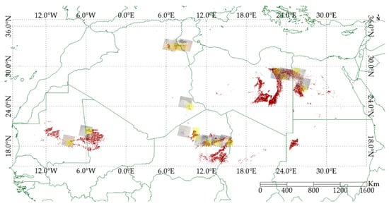
Figure 1.
Cluster 13 pixels across North Africa. The red color represents Cluster 13 pixels, the yellow box represents Sentinel image footprint and the images lying on the Cluster 13 pixels are the Landsat 8 images for 15 path/row(s).
3.2. Process
After the selection of the cluster, the data of the selected cluster from two sensors for cross-calibration were acquired and filtered for cloud pixels. Digital Number (DN) values given by Landsat and the TOA reflectance form Sentinel Level 1 product data were converted and scaled, respectively, to obtain the top of atmosphere (TOA) reflectance values for each sensor. One of two sensors was selected as a reference sensor for calibrating the other one and the spectral response of these two sensors was matched by calculating the spectral band adjustment factor (SBAF) and applying it on the sensor undergoing calibration. After the SBAF correction, both the sensors were normalized to minimize the bidirectional reflectance distribution function (BRDF) effect, and the data trend for both the sensor was determined and the cross-calibration gain was estimated, which is described as follows.
3.2.1. Cloud Filtering and Outlier Removal
OLI and ETM+ image data were acquired and the images with more than 40% cloudy and shadowed pixels were discarded for further analysis, similar for the MSI (Sentinel2A and Sentinel 2B) image data. For Landsat 7 and Landsat 8, band quality assessment (BQA) data were used to create a binary mask to filter out the outliers and, for Sentinel data, a binary cloud mask was implemented for each resolution. A few images which behaved as outliers were further filtered by visual inspection. Out of the 16 path/row(s) suggested by Hasan [24], path/row 178/47 was discarded, as images for this path/row showed persistent storms. Cluster 13 zone-specific binary masks were created, as explained by Hasan, and pixels of the filtered images that did not lie on Cluster 13 pixels within the selected 15 path/row(s) were excluded.
3.2.2. Conversion of Image Data to TOA Reflectance
OLI and ETM+ image data were converted to TOA reflectance using the rescaling coefficients obtained in the metadata file, as given by Equation (1)
where is the Landsat level 1 product TOA reflectance with solar zenith angle cosine correction; and are the band-specific multiplicative and additive scaling factors, respectively, obtained from the metadata file; is the quantized and calibrated standard product pixel value (DN); and is the solar zenith angle per pixel, as extracted from the associated product solar angle band.
Similarly, the reflectance for the filtered MSI images was calculated by using Equation (2)
where is the MSI Level 1 product TOA reflectance, is the quantized and calibrated standard product pixel value (DN), and k is the reflectance scaling factor (quantization value) obtained from the metadata file.
3.2.3. Estimation of Spectral Band Adjustment Factor
Each of the sensors has a different spectral response, which needs to be compensated by some factor so that the reflectance of any of the two sensors can be compared with each other. The compensating factor for cross-calibration is described in this section.
The satellite sensors used for cross-calibration have different spectral responses even when the sensors look at the same target through similar spectral regions. These differences in spectral response can contribute to a systematic band offset when cross-calibration is performed. Therefore, compensation for these differences should be accounted for better cross-calibration, for which we require prior knowledge of the spectral signature of the target. This compensating factor is known as the spectral band adjustment factor (SBAF), which considers the spectral profile of the target and the relative spectral response (RSR) of the sensor [6].
In this work, six different combinations of cross-calibration were used. For each combination, one sensor was chosen as a “reference” sensor, which was assumed to be well-calibrated, and another as the sensor “to be calibrated”. The SBAF was applied to the latter sensor to match its spectral response with the response of the reference sensor, and is given by
where and are, respectively, the simulated TOA reflectances for the reference sensor and the sensor to be calibrated; is the hyperspectral profile of the surface; and and is the relative spectral response of the reference sensor and the sensor to be calibrated.
The simulated TOA reflectance was obtained by integrating the RSR of the multispectral sensor with the hyperspectral profile of the target at each sampled wavelength, as shown in Equation (3).
The TOA reflectance of the sensor to be calibrated was converted to the corresponding reflectance of the reference sensor using Equation (4)
where is the TOA reflectance of the sensor to be calibrated which is equivalent to the TOA reflectance of the reference sensor, and is the original TOA reflectance of the sensor to be calibrated.
The spectral profile of the target is derived from EO-1 Hyperion hyperspectral data acquired from United States Geological Survey (USGS) EarthExplorer (https://earthexplorer.usgs.gov, accessed on 1 December 2018) over Cluster 13, and pixels containing more than 10 percent of cloud pixels are discarded, along with t images with a 5 degrees look angle or greater, as described by Shrestha et al. [25]. A total of 213 hyperspectral images were obtained and were drift-corrected, along with absolute gain and bias correction [26]. Figure 2 shows the hyperspectral profiles extracted from Hyperion to estimate the hyperspectral profile of Cluster 13, where the yellow dots represent the mean hyperspectral signature.
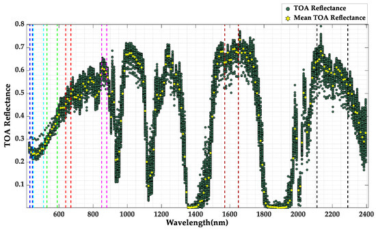
Figure 2.
Hyperspectral Data of Cluster 13. The vertical dashed lines represent the wavelength ranges of Coastal Aerosol, Blue, Green, Red, NIR, SWIR 1, and SWIR 2bands.
The SBAF corrected data were further normalized using the 15 coefficients quadratic model derived from four angles, which were also used to normalize the TOA reflectance of all the sensors, as described in the next section.
3.2.4. Bidirectional Reflectance Distribution Function Normalization
The TOA reflectance of the Earth’s surface varies with respect to the solar and viewing geometry as the surface of the Earth is non-Lambertian in nature. This effect is referred to as the Bidirectional Reflectance Distribution Function (BRDF) effect, which is contributed by the solar position that changes significantly over the season. The effect also increases as the field of view of the sensor increases and can also occur due to variations in orientation among the multiple sensors imaging the same target with the same solar position. Although OLI, ETM+, and MSI, with a narrower field of view, have lesser BRDF effects, this needs to be normalized for further analysis.
An absolute calibration BRDF model deriving linear and quadratic functions of the solar zenith angle was developed [27] using Libya 4. To fully account for the complexity of the BRDF effects, the BRDF model was developed including all the four angles as derived by Farhad et al. [28] This model converts the view and solar angles from a spherical coordinate basis to a linear Cartesian basis and obtains a TOA reflectance of the surface as a continuous function of independent variables. Kaewmanee [29] further extended the model developed by Farhad et al., using an interaction term, which characterized the BRDF model well, with better uncertainty after normalization. This 15-coefficient quadratic model has been used for this work, which is given by Equation (5)
where , , , …. are the model coefficients. Y1, X1, Y2, X2 are Cartesian coordinates representing the planar projections of the solar and sensor angles originally given in spherical coordinates.
where SZA, SAA, VZA, and VAA are the solar zenith, solar azimuth, view zenith, and view azimuth angles, respectively. The BRDF-normalized TOA reflectance for each sensor was calculated using Equation (10)
Here, is the observed mean TOA reflectance from each scene. is the model-predicted TOA reflectance, and is the TOA reflectance with respect to a set of “reference” solar and sensor position angles; for this analysis, the reference SZA, SAA, VZA, and VAA angles were chosen from the common geometry of all the sensors.
3.2.5. Data Smoothening and Trend Identification Using Modified Savitzky–Golay Filter
The proposed approach aims to utilize the cluster to understand the differences between the two sensors acquiring the data on a day-to-day basis. For this, the trend line of the data was determined after all the correction and normalization processes by applying the modified Savitzky–Golay filter. The Savitzky–Golay filter is a time-domain technique of data smoothing by low-pass filtering proposed by Savitzky and Golay, which is based on local least-squares polynomial approximation [30]. The polynomial function is given by Equation (11)
where n is the degree of the polynomial and c is the set of coefficients. The filter fits a polynomial to the sets of data in a specified window and produces an output which is the value of the polynomial in the central point of the window. For the next point, the window shifts by one day, and the process is repeated.
A moving window size of 60 days and polynomial fit of order 3 was chosen for this work, as it gave the best approximation of the data trend over time. The overall trend of the TOA reflectance of each sensor was determined and changes in trend and shifts in momentum were observed. The Savitzky–Golay filter has the peak preservation property and generates the data trend which helps to examine the patterns of the data throughout the specific period. Thus, the obtained trends were used to calculate the cross-calibration gain of the two sensors, as explained in the next step.
3.2.6. Trend-to-Trend Cross-Calibration Gain
When the measurements of two sensors corrected for SBAF and BRDF were obtained, the sensor calibration difference was evaluated using the sensor trends, which are simply obtained as the trend ratio of the two sensors, as given by Equation (12)
where is the cross-calibration gain for day, and are TOA reflectance for the two sensors for day after the application of the modified Savitzky–Golay filter.
3.2.7. Uncertainty Analysis
The cross-calibration accuracy of two sensors can be influenced by several sources of uncertainty acquired from the inherent variability in the sensors and data itself, or from the process and techniques involved in the measurement. This step accounts for these various sources of uncertainty for effective cross-calibration. For this analysis, uncertainty associated with variability of site and sensor over time, SBAF uncertainty, and BRDF uncertainty were considered as the primary sources of uncertainty. This section shows the process used to determine each source of uncertainty.
For the temporal uncertainty ), the temporal variability of the site and the temporal drift of the sensor were considered. The standard deviation of the mean TOA reflectance of each scene from each path/row was calculated for OLI and ETM+ sensors, and also for each tile of MSI images. The temporal uncertainty was then estimated as the mean of the obtained standard deviation for each sensor.
To calculate the uncertainty due to the non-uniformity of the site (variability between WRS path/row within Cluster 13), also known as the spatial uncertainty (, the temporal standard deviation of the whole cluster ( data was calculated, which would consist of the temporal component as well as the spatial variability of the site. The temporal component ) from this calculated standard deviation ( was excluded, as shown in Equation (13).
The uncertainty that occurred due to the BRDF model applied on the dataset for normalization was also considered, which is the root mean square error (RMSE) of the model to predict the surface. The difference between the measured TOA reflectance and the TOA reflectance predicted by the model is the BRDF error, as given by Equation (14). The BRDF error was calculated for each data point, and then the root mean square of these errors was estimated as the BRDF uncertainty .
Here, is the observed mean TOA reflectance from each scene. is the model-predicted TOA reflectance.
The SBAF uncertainty was determined by calculating the standard deviation of 213 SBAF values derived from the hyperspectral data of Cluster 13.
The overall uncertainty of the gain, including the calibration uncertainty ( of each sensor, was calculated by using Equation (15), and each source of uncertainty calculated for the sensor pairs is further discussed in Section 4.4.
4. Results
This section shows the result of each step explained in the methodology. Cross-calibration of each pair of the sensor was performed and is shown here. First, this compares the SBAF values derived for each pair of cross-calibration and shows how SBAF significantly adjusts the two sensor’s RSR mismatch. Then, the outcome of the implementation of the full BRDF model is discussed. Then, the following subsection shows the trends identified with the implementation of the modified Savitzky–Golay filter to cross-calibrate the two sensors. Finally, it gives the summary of the cross-calibration gains for each pair of sensors, along with the uncertainty associated with the cross-calibration gains.
4.1. Spectral Band Adjustment Factor for Cluster 13
Sets of SBAFs were estimated from 213 hyperspectral profiles derived from Cluster 13, and the average SBAF estimated for each pair of the sensors is as shown in Figure 3. The SBAF values shown are the compensating factor for all the sensors to be calibrated according to the reference sensor.
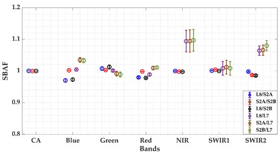
Figure 3.
Spectral Band Adjustment Factors derived from the hyperspectral profile of Cluster 13 for each sensor pair (error bars represents the standard deviation at k = 2. The sensor in the numerator is the reference sensor for each combination).
The SBAFs values derived for MSI-A and MSI-B are closer to unity, since the relative spectral response of these sensors is very similar, as seen in Figure 4. There is a small deviation of about 1.3% for the SWIR 2 band because there is a relative shift in the RSR of MSI-A and MSI-B sensors for SWIR 2 bands when compared to the other bands. Similarly, the SBAF values obtained for Landsat 8 OLI paired with Sentinel 2A exhibited similar SBAF values when compared to the SBAF for OLI and MSI-B pair, since the RSR mismatch of MSI A and MSI B with OLI is similar for the corresponding bands. It can be observed from the RSR plot for Landsat 8 OLI and Sentinel MSI that the blue, green, and red bands have a relative shift in RSR, because of which the SBAF for these two bands highly deviates from the unity, up to 3%. A larger deviation from unity is observed for the pairs involving the Landsat 7 ETM+ sensor. When comparing the RSR of the Landsat 8 OLI sensor and Landsat 7 ETM+ sensor, for NIR, SWIR1 and SWIR 2 channel, the spectral response of ETM+ is significantly wider than the OLI sensor. The RSR of ETM+ is wider when compared to all the other remaining sensors, which caused the SBAF values to highly deviate from one. This high deviation is observed in the NIR band, which is as large as 9% for all the sensor pairs with Landsat 7. Additionally, the error bars for these bands are larger because of the RSR shift and width mismatch of RSR between the two sensors.
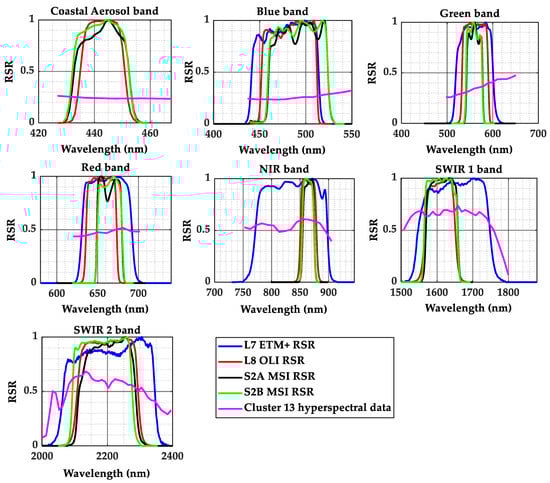
Figure 4.
Relative Spectral Response (RSR) of Landsat 7 ETM+, Landsat 8 OLI, Sentinel 2A MSI, Sentinel 2B MSI and the derived hyperspectral profile of Cluster 13.
The calculated SBAF was applied to all the corresponding sensors that were to be calibrated, to match them with their respective reference sensor. As an example, the SBAF-corrected mean TOA reflectance of Landsat 7, to match it with Sentinel 2A, is shown in Figure 5. The observed mean TOA reflectance of Landsat 7 represented by the blue symbol slightly deviates from the observed TOA reflectance of Sentinel 2A, which is represented by the black symbol. Particularly, when comparing this to the NIR band, the mean TOA reflectance of Landsat 7 does not cross the error bars of the mean TOA reflectance of Sentinel 2A and differs by 0.05 reflectance units. Similarly, there is a difference in the SWIR 2 band by 0.02 reflectance units. These differences are due to the RSR mismatch of the two sensors, which is compensated by SBAF. After the SBAF correction, the mean TOA reflectance of Landsat 7 represented by red dots is similar to the TOA reflectance of Sentinel 2A. The mean values are within the error bars, which shows that the RSR mismatch has been compensated by the implementation of the spectral band adjustment factor.
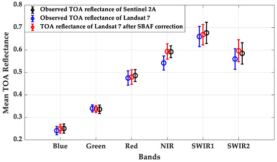
Figure 5.
Comparison of TOA reflectance of Landsat 7 before and after the SBAF correction for the cross-calibration combination of Sentinel 2A and Landsat 7. (The error bars represent the standard deviation, k = 2).
4.2. BRDF Normalization of the TOA Reflectance of the Sensor
Since the directional effect is related to the target, a single BRDF model was used to predict Cluster 13. For this, a set of common reference angles was selected in such a way that the TOA reflectance of the sensors is scaled to a common level. Thus, the selected reference solar zenith, solar azimuth, view zenith, and view azimuth angles are , , and 1 respectively. These angles were used to determine the polar projections of the view and solar angles to calculate the reference reflectance of the dataset. Similarly, the model-predicted TOA reflectance was calculated using the angles of the corresponding scene. Figure 6 demonstrates an example of the BRDF model, predicting the TOA reflectance where the BRDF model predicting the TOA reflectance of the Sentinel 2A for the NIR band is shown. It can be seen from the figure that the model predicts the data well, with the mean residual error of −0.0672%. For all the sensor data, the model predicted the nature of the target well, with residual errors very close to zero.
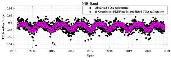
Figure 6.
Comparison of the observed top of atmosphere (TOA) reflectance and the TOA reflectance predicted by the BRDF model.
After the generation of the model, the BRDF-normalized TOA reflectance was obtained by scaling the reference reflectance. Figure 7 shows how the directional effects of the site were improved after applying the model on the data by comparing the observed TOA reflectance and the normalized TOA reflectance for Sentinel 2A, the NIR band. It can be observed from the figure that the seasonal oscillatory pattern of the TOA reflectance of Sentinel has substantially reduced.
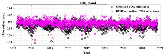
Figure 7.
Comparison of the observed TOA reflectance and the bidirectional reflectance distribution function (BRDF)-normalized TOA reflectance of Sentinel 2A.
4.3. Data Trend Identification with Daily Coincident Acquisitions
Figure 8 and Figure 9 show the TOA reflectance of daily coincident observation obtained from Landsat 8 and Sentinel 2A for the red band, which is represented by red dots. These data represent the trend line detected by the Savitzky–Golay filter and the data interpolated every day throughout the 5 years. The detected trend follows the corrected TOA reflectance data of Landsat 8 and Sentinel 2A, represented by the black dots. With the proper window size of 60 and the polynomial order of 3, some of the outliers have been filtered out, maintaining the original trend of the data.
Figure 8.
Landsat 8 trend with the daily acquisition (red dots represent the trend line detected by the Savitzky–Golay filter applied on the black dots, which is the BRDF-normalized TOA reflectance of Landsat 8).
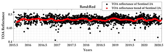
Figure 9.
Sentinel 2A trend with the daily acquisition (red dots represent the trend line detected by the Savitzky–Golay filter applied on the black dots, which is the spectral band adjusted factor (SBAF)-corrected and BRDF-normalized TOA reflectance of Sentinel 2A).
Figure 10 shows a comparison of the trends of Landsat 8 and Sentinel 2A for all the bands. Since Sentinel 2A accounted for the compensation of RSR mismatch with Landsat 8 after SBAF correction, the TOA reflectance of the two sensors is expected to be similar for the same target.
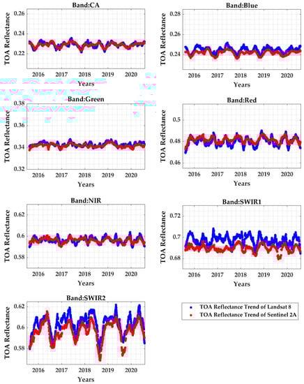
Figure 10.
Comparison of Landsat 8 OLI and Sentinel 2A MSI TOA reflectance trend.
As expected, TOA reflectance for both of the sensors follows a similar pattern, and they also lie on top of each other, especially in coastal aerosol, green and NIR band. Landsat 8 and Sentinel 2A are believed to be well-calibrated sensors and, therefore, an excellent agreement can be seen between these two sensor’s data trends. The best agreement is seen in the green band, where the TOA reflectance of the two sensors lies approximately within 0.2%.
Even after the application of the smoothing filter, and using the methodology on a day-to-day basis, some data spreads are detected in the trend line because of the lower amount of data contained within the specified window for interpolation. Few outliers within the sliding window contributed to some high and low peaks in the trend. This can be seen more clearly in the SWIR 2 channel in the middle of every year, for both of the sensors, where the trend line has a low peak because of the few low datapoints within the Savitzky–Golay window. There are variations in the order of 2 to 3 reflectance units observed throughout the year on the cluster, which are captured by both the sensors. Therefore, the two sensors are closely tracking each other using data from a different portion of the continent.
Similar trends were captured with the use of a modified Savitzky–Golay filter for all the sensors, and for all the bands. The trends of all the sensors were then used to detect the differences between the sensor pairs.
4.4. Cross-Calibration Gain with Their Uncertainties
The instantaneous ratio of the trends in the sensor data was obtained for each pair of OLI, ETM+, and MSI sensors, and the obtained values are shown in this section. The cross-calibration gain for different combinations of sensors is estimated, which is shown in Figure 11, Figure 12, Figure 13, Figure 14, Figure 15 and Figure 16. The cross-calibration gain is centered around one, and the sensors for each pair agree to better than 2.5% for all the bands. Landsat 8 and Sentinel 2A were considered as highly calibrated sensors and, with this approach, the difference between these two sensors is found to be within 1% for all the bands. Similarly, the difference between the twin satellite sensors MSI-A and MSI-B is found to be within 1%, since these two sensors are identical sensors orbiting in the same orbit. The cross-calibration results of Landsat 8 and Sentinel 2B show that these two sensors agree to better than 1% in all the bands, except for the blue band, which is around 2%. Furthermore, the cross-calibration of the ETM+ sensor with the other three sensors shows agreement within 2.5%.
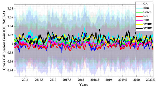
Figure 11.
The trend-to-trend cross-calibration gain of Landsat 8 OLI and Sentinel 2A MSI. The shaded region is the uncertainty for individual bands.
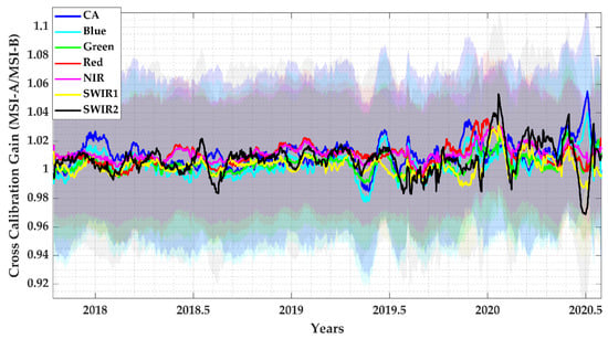
Figure 12.
The trend-to-trend cross-calibration gain of Sentinel 2A MSI and Sentinel 2B MSI. The shaded region is the uncertainty for individual bands.
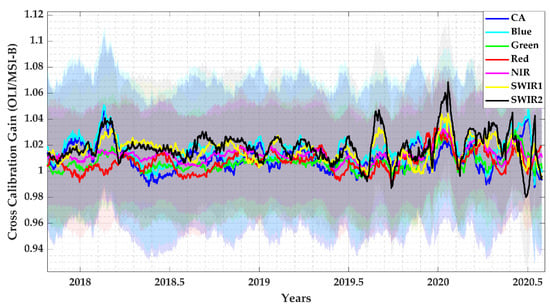
Figure 13.
The trend-to-trend cross-calibration gain of Landsat 8 OLI and Sentinel 2B MSI. The shaded region is the uncertainty for individual bands.
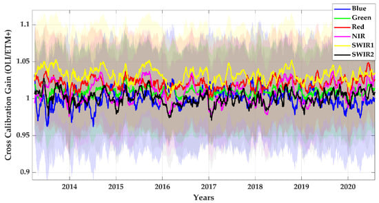
Figure 14.
The trend-to-trend cross-calibration gain of Landsat 8 OLI and Landsat 7 ETM+. The shaded region is the uncertainty for individual band.
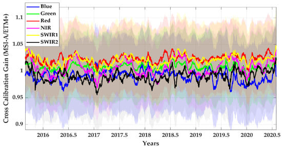
Figure 15.
The trend-to-trend cross-calibration gain of Sentinel 2A MSI and Landsat 7 ETM+. The shaded region is the uncertainty for individual bands.
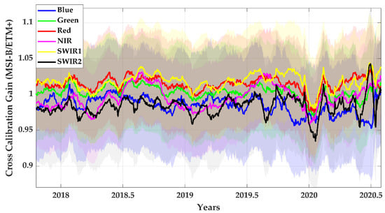
Figure 16.
The trend-to-trend cross-calibration gain of Sentinel 2B MSI and Landsat 7 ETM+. The shaded region is the uncertainty for individual bands.
The shaded region on the graphs shows the uncertainty for each band. As mentioned earlier, different sources of uncertainty were computed and, as an example, the sources of uncertainty calculated for the cross-calibration of Landsat 8 and Sentinel 2A are shown in Table 2. For this cross-calibration pair, the major contributor to the type A uncertainty is the BRDF model uncertainty, which is around 3.5% for the coastal aerosol and blue band. Since BRDF normalization primarily considers the ground-level effects, the changes in the sky are not modeled as well; thus, normalization is not as effective in the blue channel contributing to the larger uncertainty source in these channels. This case is similar to all the other sensor pairs. The uncertainty in the SBAF values is lower, no more than 0.3%. The temporal and the spatial uncertainty of the cluster is similar for all the sensor pairs. The temporal uncertainty changes with the temporal standard deviation of the sensor for other cross-calibration pairs. The overall uncertainty is also affected by the calibration uncertainty for each cross-calibration pair. For OLI and MSI-A pair, the total uncertainty was within 6%.
Table 2.
Sources of uncertainty for the cross-calibration of Landsat 8 and Sentinel 2A.
Similarly, for other sensor combinations, the highest uncertainty is observed in shorter wavelengths, which were within 6–8%. The uncertainty for the cross-calibration of Landsat 7 is higher because of the calibration uncertainty of Landsat 7, which is around 5% [31]. Additionally, the SWIR channel has a higher uncertainty, similar to the shorter wavelength bands, since the TOA reflectance for the two sensors varies in this bands. NIR band has the lowest uncertainty among all the bands for all the combinations, which range from 3 to 7%. The gains, along with their uncertainties, are summarized in Table 3.
Table 3.
The trend-to-trend cross-calibration summary.
Despite the larger uncertainties, the overall cross-calibration gain is within an accuracy of 2.5%. Additionally, the ratio of the trends of the data from a different portion of North Africa shows the differences in the satellite, not the differences which contributed to looking at different parts of the continent, since the variations in the sites are captured by both the sensors.
5. Validation of the New Cluster-Based Approach
This section validates the new approach of the trend-to-trend cross-calibration by comparing this approach with the traditionally accepted PICS-based cross-calibration. The cross-calibration of Landsat 8 and Sentinel 2A is shown as an example, since these sensors are highly effective for data interoperability. Kaewmanee [23] performed the cross-calibration of Landsat 8 and Sentinel 2A using Libya 4 CNES ROI, with coincident and near-coincident scene pairs deriving the hyperspectral profile of Libya 4 without considering the drift and bias correction of the Hyperion data. For the validation purposes, this work utilizes the result of the traditional PICS-based approach performed by Kaewmanee after updating the hyperspectral data using the same Libya 4 CNES ROI, comparing it with the new cluster-based approach. The results of the traditional PICS used for the comparison are obtained via communication with the author.
For the cross-calibration of Landsat 8 and Sentinel 2A, the data from both the satellites were considered, since the launch of Sentinel 2A. The total number of cloud-free acquisitions obtained for Landsat 8 was 1142 and for sentinel 2A was 1582. The TOA reflectance of each sensor was determined and the SBAF was calculated for MSI, considering Landsat 8 as the reference sensor for the cross-calibration.
5.1. Spectral Band Adjustment Factor for Libya 4 ROI and Cluster 13
For the PICS-based approach using Libya 4, sets of SBAF were derived using 360 hyperspectral data profiles, and, for Cluster 13, sets of SBAFs were estimated from 213 hyperspectral profiles. Since Libya 4 is a part of Cluster 13, similar results of the hyperspectral profile are expected. Therefore, SBAF values retrieved from similar hyperspectral profiles are also expected to be similar. The average SBAF estimated for both approaches is shown in Figure 17.
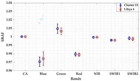
Figure 17.
Spectral Band Adjustment Factor (SBAF) for Sentinel 2A MSI for Libya 4 ROI and Cluster 13 (error bars represent the standard deviation, k = 2).
The SBAFs derived from the hyperspectral signature of Libya 4 and Cluster 13 are similar to each other. The SBAF values of coastal aerosol, NIR, SWIR1, and SWIR2 bands are close to 1, since their RSRs are similar to each other. For blue, green, and red bands, a relative shift in RSR can be observed, meaning that the SBAF for these two bands highly deviates from unity. Comparing the SBAF obtained from Libya 4 ROI and Cluster 13, the SBAF values are equal for all the bands, except for the blue and green band, where the observed differences in the two approaches are around 0.37% and 0.30%. These differences could be due to the differences in the hyperspectral profile of Libya 4 ROI and Cluster 13, and also due to the width difference of the RSR. Additionally, the error bars for blue, green, and red bands are larger because of the RSR shift and width mismatch of RSR between the two sensors. The coefficient of variation of red bands is similar for both Cluster 13 and Libya 4, which was approximately 1.11%, whereas, for the green band, the coefficient of variation for Cluster 13 is 0.29%, and for Libya 4 ROI was 0.2%.
5.2. Cluster-Based Trend Totrend Cross-Calibration vs. Traditional PICS-Based Cross-Calibration Gain along with the Associated Uncertainty
Using the trend of the TOA reflectance of the two sensors, as shown in Figure 10, the cross-calibration gain was calculated as the ratio of the OLI TOA reflectance trend to the MSI TOA reflectance trend. The resulting gain values are shown in Figure 18. Since Libya 4 is included within Cluster 13, the cluster-based trend-to-trend cross-calibration gain ratio is similar to the PICS-based coincident scene pair approach. The gain values derived from the traditional PICS-based cross-calibration seem to have more stability throughout time. Additionally, the uncertainty of Libya 4 is less than that of Cluster 13, which causes lower scatteredness in the gain derived from Libya 4. However, the cross-calibration gain seems to follow a similar pattern, lying on top of each other. The cross-calibration gain for blue, green, red, and NIR band has gain values near unity, since the TOA reflectance of the two sensors for these bands have a better agreement. The cross-calibration gain derived from Libya 4 and Cluster 13 are also equal for the green, red, and NIR bands and lies inside the uncertainty range. The relative difference between the gain derived from Libya 4 and Cluster 13 is larger in the coastal aerosol and blue band, which is approximately within 2%.
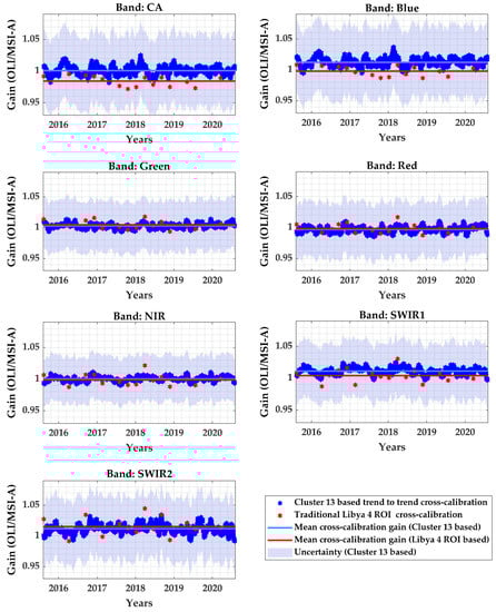
Figure 18.
Comparison of Landsat 8 and Sentinel 2A MSI cross-calibration gain ratio with cluster and PICS-based approach.
The sources of uncertainty were defined for the calculation of the cross-calibration gain, as discussed earlier in Section 4.4, and the gain obtained with the traditional approach of cross-calibration, was compared, as shown in Figure 18. The summary of type A and type B uncertainties sources for the cross-calibration of Landsat 8 and Sentinel 2A is shown in Table 2. The type A uncertainty source includes the temporal, spatial, BRDF, and SBAF uncertainty, and the type B uncertainty is the calibration uncertainties associated with the sensors. The calibration uncertainties of OLI and MSI are 2% [18] and 2.5% [10], respectively, which are the major contributors to the final uncertainty. The total uncertainty calculated for the cross-calibration between OLI and MSI-A sensor is within 5.8% for all the bands.
Figure 19 shows the mean cross-calibration gain ratio and the associated standard deviation derived for the previous and current approach to cross-calibration. The mean cross-calibration for the trend-to-trend approach was calculated by taking an average of the blue data in Figure 18 and, for the Libya 4 coincident scene, pairs approaching the mean cross-calibration gain were calculated by taking the average of the red datapoints in Figure 18. The black data in Figure 19 were derived by Farhad et al. [28] for the cross-calibration of OLI and MSI sensors using PICS, where the error bars represent the uncertainty derived, which was approximately 6.8%. For two perfectly calibrated sesnors, the value of the cross-calibration gain ratio is expected to be unity. However, for some bands, the cross-calibration ratios deviate from unity due to various factors, such as the uncertainties associated with SBAF correction, BRDF normalization, sensor instability, and the atmosphere. As a whole, both approaches showed consistent estimation of the cross-calibration ratios, since the error bars cross the mean values. The cross-calibration gain derived from Cluster 13 shows higher uncertainties than the Libya 4 ROI-derived cross-calibration gain. Since Farhad et al. also derived the cross-calibration gain, combining various PICS locations, the uncertainty is much larger than the other two cross-calibration ratios. The uncertainty from the cluster-based approach has a larger uncertainties in the coastal aerosol and blue band, which is approximately 6%, and has the lowest uncertainty for the NIR band, which is within 4%. The SWIR channel has a larger uncertainty for both approaches, since the TOA reflectance of Landsat 8 and Sentinel 2A has more variation in these channels.
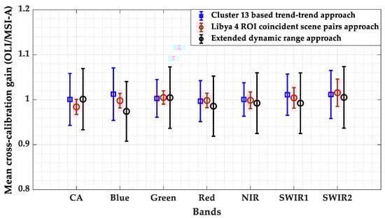
Figure 19.
Cross-calibration gains comparison of Landsat 8 OLI and Sentinel 2A MSI using a traditional ROI-based approach and the cluster-based approach. (Blue and black bars represents the uncertainty and the red bar is the associated standard deviation at k = 2).
These cross-calibration results show a comparison of traditional and current approaches to the cross-calibration of Landsat 8 and Sentinel 2A, which exhibited consistent results, within 2%, and the gains derived from Libya 4 ROI and Cluster 13 are very close to each other. Coincident scene pairs of Landsat 8 and Sentinel 2A were used for the traditional cross-calibration, which shows that traditional cross-calibration is achieved well with the coincident scenes. Considering the higher uncertainties of the cluster-based approach, both the previous and the proposed methods provide consistent results of cross-calibration and they are statistically equal.
Similarly, sensor pairs that are out-of-phase and unable to achieve coincident scene pairs can be cross-calibrated using near-coincident scene pairs [8]. To compare the current approach with the traditional cross-calibration using near-coincident scene pairs, the comparison of cross-calibration results of Sentinel 2A and Sentinel 2B was also made, as shown in Figure 20. The cross-calibration gain obtained with the scene pairs of Libya 4 ROI (5 days apart) from the MSI-A sensor and MSI-B sensor is represented by the red dots and the cross-calibration gain, with the cluster-based trend-to-trend approach represented by the blue dots. The red data, from the traditional PICS approach, were obtained via personal communication with the author [23]. The black line represents the cross-calibration result obtained by Charlotte Revel et al. [32], with the cross-calibration over desert sites. Comparing the mean values of all the three approaches, it can be seen that the mean values of the previous cross-calibration lie within the uncertainty range of the proposed Cluster 13-based approach. From the graph, it can be observed that the gain obtained from near coincident scene pairs has more variability than the one where coincident scene pairs were used. However, results obtained from the new trend-to-trend approach with cluster showed consistent results with the near-coincident scene pair approach for the cross-calibration of Sentinel 2A and Sentinel 2B, which is within 1% for all the bands and 2.5% for the coastal aerosol band. This shows the major advantage of the proposed approach when it comes to cross-calibrating two sensors that cannot acquire coincident scenes.
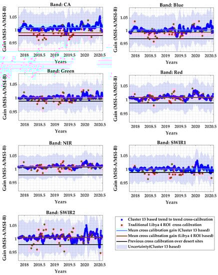
Figure 20.
Comparison of Sentinel 2A and Sentinel 2B MSI cross-calibration gain ratio with cluster- and PICS-based approach.
6. Discussion
The cross-calibration of satellites is performed to provide accurate and consistent results between multiple sensors over the land surface. It plays an important role in putting sensors into a common radiometric level for mission continuity and interoperability [6]. Traditionally, coincident scene/near-coincident scene pairs from various PICS locations have been used to cross-calibrate any two sensors. This PICS-based approach can possibly obtain Landsat 8 and Sentinel 2A coincident acquisitions every 80 days, because of the difference in the respective satellite orbital patterns [22]. Among the few available locations on Earth, Libya 4 can provide these acquisitions. For cross-calibration based on the coincident scene pair approach of Landsat 8 and Sentinel 2A, only 15 coincident scene pairs were acquired over 5 years. Shrestha et al. [16] used clusters to increase the frequency of datasets used for cross-calibration and obtained only 11 coincident scene pairs in a year. With this trend-to-trend cross-calibration approach, applying the Savitzky-Golay filter and interpolating it each day, for a period randing 2015 to 2020, 1815 daily coincident scene pairs were obtained, and the differences between Landsat 8 and Sentinel 2A were better observed at a frequency greater than 80 days. Therefore, within a shorter period, trend-to-trend cross-calibration helps in understanding the sensor’s differences, making it possible to detect and correct these changes in a shorter time frame. This method is highly useful when calibrating a newly launched satellite whose calibration needs to be done within a shorter calibration time, and where enough coincident or near-coincident scene pairs cannot be achieved within the calibration period.
The Savitzky–Golay filter was used to determine the trend of the TOA reflectance of Cluster 13 for this work, which seems to predict the trend more accurately if there are enough data within the Savitzky–Golay window span. Missing data or data gaps in the TOA reflectance could produce more spreads and variations in the detected trend. In Figure 20, a spread of about 0.08 reflectance can be observed in SWIR 2 band since, for Sentinel 2B, there were only four datapoints within the 60 day window, which produced the high data spread at around the end of the year 2019. Additionally, the analysis is based on the time domain filter, which can be further analyzed with different techniques of time-domain and frequency-domain filtering processes. Even more accurate and real trends can be identified with better smoothing filters.
The proposed technique of cross-calibration showed that the cross-calibration results of Landsat 8 and Sentinel 2A are within 1% and consistent with the results obtained from Libya 4 CNES ROI using coincident scenes. From Figure 20, it can be observed that the gain obtained from near-coincident scene pairs has more variability than the one where coincident scene pairs were used. However, results obtained from the new trend-to-trend approach with cluster showed consistent results for the cross-calibration of Sentinel 2A and Sentinel 2B. The result is within 2% when compared to the traditional Libya 4 ROI cross-calibration results. This shows the major advantage of the proposed system when it comes to cross-calibrating two sensors whose coincident scene pairs cannot be achieved.
7. Conclusions
Since Cluster 13 provides higher temporally frequent sets of data for the cross-calibration of two sensors, the proposed trend-to-trend cross-calibration technique further amplifies this opportunity. The purpose of this EPICS-based trend-to-trend cross-calibration is to illustrate the technique of using the cluster to cross-calibrate two satellite sensors without needing coincident or near-coincident acquisitions. The obtained results have been shown and compared to the previously accepted approach, which showed consistent and statistically equal results. Out of all the other bands for all the combinations of sensors for cross-calibration, the NIR band showed a better agreement when compared to the coincident, near-coincident scene pair approach, which was within 1%. Maximum offsets were observed in coastal aerosol, blue and SWIR1 channels, and were within 2.5%. The uncertainties in these bands were higher, which was mostly due to the spatial uncertainty of Cluster 13, the calibration uncertainty, and the BRDF effects’ uncertainty. However, the overall cross-calibration is comparable to the traditional approach. Based on the results of EPICS based cross-calibration, it can be concluded that any portion of cluster 13 can be used for cross calibrating two sensors in much shorter time, using the trends of two sensors, with the same level of accuracy as provided by the traditional PICS-based method that utilizes coincident or near coincident scene pairs.
Author Contributions
Conceptualization, P.K. and L.L.; Formal analysis, M.K. and C.T.P.; Funding acquisition, L.L.; Methodology, P.K.; Supervision, L.L.; Validation, P.K. and M.K.; Visualization, L.L.; Writing—original draft, P.K.; Writing—review and editing, L.L. All authors have read and agreed to the published version of the manuscript.
Funding
USGS EROS (grant number G19AS00001).
Data Availability Statement
Landsat 8 and Landsat 7 courtesy of the US Geological Survey Collection 2 Landsat 8-9 OLI/TIRS Digital Object Identifier (DOI) number: /10.5066/P975CC9B. Sentinel 2A and Sentinel 2B image courtesy of the US Geological Survey. Sentinel-2 Digital Object Identifier (DOI) number: /10.5066/F76W992G.
Acknowledgments
The authors would like to thank all the members of the Image Processing lab, SDSU for their continuous support and guidance.
Conflicts of Interest
The authors declare no conflict of interest.
References
- Barrientos, C.; Mattar, C.; Nakos, T.; Perez, W. Radiometric Cross-Calibration of the Chilean Satellite FASat-C Using RapidEye and EO-1 Hyperion Data and a Simultaneous Nadir Overpass Approach. Remote Sens. 2016, 8, 612. [Google Scholar] [CrossRef]
- Wang, D.; Morton, D.; Masek, J.; Wu, A.; Nagol, J.; Xiong, X.; Levy, R.; Vermote, E.; Wolfe, R. Impact of sensor degradation on the MODIS NDVI time series. Remote Sens. Environ. 2012, 119, 55–61. [Google Scholar] [CrossRef]
- Dinguirard, M.; Slater, P.N. Calibration of space-multispectral imaging sensors: A review. Remote Sens. Environ. 1999, 68, 194–205. [Google Scholar] [CrossRef]
- Sterckx, S.; Livens, S.; Adriaensen, S. Rayleigh, deep convective clouds, and cross-sensor desert vicarious calibration validation for the PROBA-V mission. IEEE Trans. Geosci. Remote Sens. 2013, 51, 1437–1452. [Google Scholar] [CrossRef]
- Cosnefroy, H.; Leroy, M.; Briottet, X. Selection and characterization of Saharan and Arabian desert sites for the calibration of optical satellite sensors. Remote Sens. Environ. 1996, 58, 101–114. [Google Scholar] [CrossRef]
- Chander, G.; Mishra, N.; Helder, D.L.; Aaron, D.B.; Angal, A.; Choi, T.; Xiong, X.; Doelling, D.R. Applications of spectral band adjustment factors (SBAF) for cross-calibration. IEEE Trans. Geosci. Remote Sens. 2012, 51, 1267–1281. [Google Scholar] [CrossRef]
- Chander, G.; Mishra, N.; Helder, D.L.; Aaron, D.; Choi, T.; Angal, A.; Xiong, X. Use of EO-1 Hyperion data to calculate spectral band adjustment factors (SBAF) between the L7 ETM+ and Terra MODIS sensors. In Proceedings of the 2010 IEEE International Geoscience and Remote Sensing Symposium, Piscataway, NJ, USA, 25–30 July; pp. 1667–1670.
- Bacour, C.; Briottet, X.; Bréon, F.-M.; Viallefont-Robinet, F.; Bouvet, M. Revisiting Pseudo Invariant Calibration Sites (PICS) over sand deserts for vicarious calibration of optical imagers at 20 km and 100 km scales. Remote Sens. 2019, 11, 1166. [Google Scholar] [CrossRef]
- Helder, D.L.; Basnet, B.; Morstad, D.L. Optimized identification of worldwide radiometric pseudo-invariant calibration sites. Can. J. Remote Sens. 2010, 36, 527–539. [Google Scholar] [CrossRef]
- Barsi, J.A.; Alhammoud, B.; Czapla-Myers, J.; Gascon, F.; Haque, M.O.; Kaewmanee, M.; Leigh, L.; Markham, B.L. Sentinel-2A MSI and Landsat-8 OLI radiometric cross comparison over desert sites. Eur. J. Remote Sens. 2018, 51, 822–837. [Google Scholar] [CrossRef]
- Farhad, M. Cross Calibration and Validation of Landsat 8 OLI and Sentinel 2A MSI. Master’s Thesis, South Dakota State University, Brookings, SD, USA, 2018. Available online: https://openprairie.sdstate.edu/etd/2687/ (accessed on 15 April 2021).
- Pinto, C.; Ponzoni, F.; Castro, R.; Leigh, L.; Mishra, N.; Aaron, D.; Helder, D. First in-flight radiometric calibration of MUX and WFI on-board CBERS-4. Remote Sens. 2016, 8, 405. [Google Scholar] [CrossRef]
- Doelling, D.; Helder, D.; Schott, J.; Stone, T.; Pinto, C. Vicarious calibration and validation. In Reference Module in Earth Systems and Environmental Sciences. Comprehensive Remote Sensing; Elsevier: Amsterdam, The Netherlands, 2018; Volume 1, pp. 475–518. [Google Scholar]
- Vuppula, H. Normalization of Pseudo-Invariant Calibration Sites for Increasing the Temporal Resolution and Long-Term Trending. Master’s Thesis, South Dakota State University, Brookings, SD, USA, 2017. Available online: https://openprairie.sdstate.edu/etd/2180/ (accessed on 15 April 2021).
- Shrestha, M.; Leigh, L.; Helder, D. Classification of North Africa for Use as an Extended Pseudo Invariant Calibration Sites (EPICS) for Radiometric Calibration and Stability Monitoring of Optical Satellite Sensors. Remote Sens. 2019, 11, 875. [Google Scholar] [CrossRef]
- Shrestha, M.; Hasan, M.; Leigh, L.; Helder, D. Extended Pseudo Invariant Calibration Sites (EPICS) for the Cross-Calibration of Optical Satellite Sensors. Remote Sens. 2019, 11, 1676. [Google Scholar] [CrossRef]
- Irons, J.R.; Dwyer, J.L.; Barsi, J.A. The next Landsat satellite: The Landsat data continuity mission. Remote Sens. Environ. 2012, 122, 11–21. [Google Scholar] [CrossRef]
- Markham, B.; Barsi, J.; Kvaran, G.; Ong, L.; Kaita, E.; Biggar, S.; Czapla-Myers, J.; Mishra, N.; Helder, D. Landsat-8 operational land imager radiometric calibration and stability. Remote Sens. 2014, 6, 12275–12308. [Google Scholar] [CrossRef]
- Goward, S.N.; Masek, J.G.; Williams, D.L.; Irons, J.R.; Thompson, R. The Landsat 7 mission: Terrestrial research and applications for the 21st century. Remote Sens. Environ. 2001, 78, 3–12. [Google Scholar] [CrossRef]
- Andrefouet, S.; Bindschadler, R.; Brown.d.Colstoun, E.; Choate, M.; Chomentowski, W.; Christopherson, J.; Doorn, B.; Hall, D.; Holifield, C.; Howard, S. Preliminary Assessment of the Value of Landsat-7 ETM+ Data Following Scan Line Corrector Malfunction. United States Geological Survey (USGS), 2003. Available online: https://www.usgs.gov/media/files/preliminary-assessment-value-landsat-7-etm-slc-data (accessed on 15 April 2021).
- Drusch, M.; del Bello, U.; Carlier, S.; Colin, O.; Fernandez, V.; Gascon, F.; Hoersch, B.; Isola, C.; Laberinti, P.; Martimort, P. Sentinel-2: ESA’s optical high-resolution mission for GMES operational services. Remote Sens. Environ. 2012, 120, 25–36. [Google Scholar] [CrossRef]
- Li, J.; Roy, D.P. A global analysis of Sentinel-2A, Sentinel-2B and Landsat-8 data revisit intervals and implications for terrestrial monitoring. Remote Sens. 2017, 9, 902. [Google Scholar]
- Kaewmanee, M. PICS Trending Analysis: S2A, S2B. Presented at the Landsat 8th Technical Interchange Meeting [Online]. January 2020. [Google Scholar]
- Hasan, M.N.; Shrestha, M.; Leigh, L.; Helder, D. Evaluation of an Extended PICS (EPICS) for Calibration and Stability Monitoring of Optical Satellite Sensors. Remote Sens. 2019, 11, 1755. [Google Scholar] [CrossRef]
- Shrestha, M.; Hasan, N.; Leigh, L.; Helder, D. Derivation of Hyperspectral Profile of Extended Pseudo Invariant Calibration Sites (EPICS) for Use in Sensor Calibration. Remote Sens. 2019, 11, 2279. [Google Scholar] [CrossRef]
- Jing, X.; Leigh, L.; Helder, D.; Pinto, C.T.; Aaron, D. Lifetime Absolute Calibration of the EO-1 Hyperion Sensor and Its Validation. IEEE Trans. Geosci. Remote Sens. 2019, 57, 9466–9475. [Google Scholar] [CrossRef]
- Helder, D.; Thome, K.J.; Mishra, N.; Chander, G.; Xiong, X.; Angal, A.; Choi, T. Absolute radiometric calibration of Landsat using a pseudo invariant calibration site. IEEE Trans. Geosci. Remote Sens. 2013, 51, 1360–1369. [Google Scholar] [CrossRef]
- Farhad, M.; Kaewmanee, M.; Leigh, L.; Helder, D. Radiometric Cross Calibration and Validation Using 4 Angle BRDF Model between Landsat 8 and Sentinel 2A. Remote Sens. 2020, 12, 806. [Google Scholar] [CrossRef]
- Kaewmanee, M. Pseudo Invariant Calibration Sites: PICS Evolution. In Proceedings of the CALCON 2018, Utah State University, Logan, UT, USA, 18–20 June 2018. [Google Scholar]
- Savitzky, A.; Golay, M.J. Smoothing and differentiation of data by simplified least squares procedures. Anal. Chem. 1964, 36, 1627–1639. [Google Scholar] [CrossRef]
- Barsi, J.A.; Markham, B.L.; Czapla-Myers, J.S.; Helder, D.L.; Hook, S.J.; Schott, J.R.; Haque, M.O. Landsat-7 ETM+ radiometric Calibration Status. In Proceedings of the Earth Observing Systems XXI, Event: SPIE Optical Engineering + Applications, San Diego, CA, USA, 19 September 2016; p. 99720C. [Google Scholar]
- Revel, C.; Lonjou, V.; Marcq, S.; Desjardins, C.; Fougnie, B.; Coppolani-Delle Luche, C.; Guilleminot, N.; Lacamp, A.-S.; Lourme, E.; Miquel, C. Sentinel-2A and 2B absolute calibration monitoring. Eur. J. Remote Sens. 2019, 52, 122–137. [Google Scholar] [CrossRef]


Publisher’s Note: MDPI stays neutral with regard to jurisdictional claims in published maps and institutional affiliations. |
© 2021 by the authors. Licensee MDPI, Basel, Switzerland. This article is an open access article distributed under the terms and conditions of the Creative Commons Attribution (CC BY) license (https://creativecommons.org/licenses/by/4.0/).