High-Resolution Mangrove Forests Classification with Machine Learning Using Worldview and UAV Hyperspectral Data

Abstract

Mangrove forests, as important ecological and economic resources, have suffered a loss in the area due to natural and human activities. Monitoring the distribution of and obtaining accurate information on mangrove species is necessary for ameliorating the damage and protecting and restoring mangrove forests. In this study, we compared the performance of UAV Rikola hyperspectral images, WorldView-2 (WV-2) satellite-based multispectral images, and a fusion of data from both in the classification of mangrove species. We first used recursive feature elimination‒random forest (RFE-RF) to select the vegetation’s spectral and texture feature variables, and then implemented random forest (RF) and support vector machine (SVM) algorithms as classifiers. The results showed that the accuracy of the combined data was higher than that of UAV and WV-2 data; the vegetation index features of UAV hyperspectral data and texture index of WV-2 data played dominant roles; the overall accuracy of the RF algorithm was 95.89% with a Kappa coefficient of 0.95, which is more accurate and efficient than SVM. The use of combined data and RF methods for the classification of mangrove species could be useful in biomass estimation and breeding cultivation.

1. Introduction

Ecosystems are the natural environmental conditions on which all organisms in the natural world depend, rendering many important services and continuously maintaining species and genetic diversity [1]. The Earth’s three major ecosystems are wetlands, forests, and oceans, which are known as the “kidneys of the Earth,” “natural reservoirs” and “treasure troves of species,” respectively. The mangrove ecosystem is one of the most important subsystems of global wetland ecosystems and one of the most biologically rich ecosystems on Earth, so it plays a highly important function in shallow wetland ecosystems [2,3]. Mangroves are tidal wetland woody biomes consisting of evergreen shrubs or trees with mangrove plants growing in tropical and subtropical coastal intertidal zones, and are globally recognized as carbon stock-rich ecosystems that provide irreplaceable social, economic, environmental, and ecological services to humans and coastal organisms [4,5]. In terms of social and economic aspects, the mangrove is increasingly valued by decision-makers from governments, NGOs, and the general public. Growing awareness has led to numerous ecotourism sites, and mangrove museums have been established to facilitate educational and scientific research endeavors while promoting socioeconomic development. The unique biochemical properties of mangroves enable them to produce a variety of unique natural products that have high medicinal value [6]. In terms of environmental and ecological aspects, mangroves have high primary productivity and can play multiple roles such as flood and tide resistance, coastal erosion prevention, pollutant filtration, seawater purification, carbon sink, ecological improvement, and biodiversity maintenance [7,8], and are known as “natural coastal guardians,” “wave-cancelling pioneers,” and a “biological purification sieve” [9,10]. In 2000, the total global mangrove area was estimated to be 13.77 million hm², accounting for 0.7% of the world’s tropical forest area, distributed in 118 countries and regions [11]; however, according to a recent NASA study [12], the global mangrove area decreased by more than 3300 km², about 2% of the total mangrove area, by 2016, mainly due to the impact of human activities. The high population pressure in coastal areas has led to the conversion of mangroves into construction land and aquaculture ponds, one of the major reasons for the loss of mangroves [11,13,14]. According to a report by the Global Mangrove Alliance (a collective of international NGOs), the degradation of mangrove forests will continue until 2030 [15]. The global decline of mangroves will be slowed by the “Mangroves for the Future program” launched by the International Union for Conservation of Nature (IUCN) and the United Nations Development Program. Recognizing the importance of mangrove protection, the Chinese government issued a Special Action Plan for Mangrove Protection and Restoration (2020‒2025) to organize the protection and restoration of mangroves in five provinces/autonomous regions, one of which is Hainan Province, in order to safeguard the service functions and social benefits provided by mangroves in the country. As sensitive ecological indicators, mangroves require monitoring, analysis, and species distribution mapping to help us understand the ecological changes along the coastal zone and provide a theoretical basis for resource planning [16] and the prevention of the invasion of exotic species.

Mangroves grow in intertidal zones, where the complex topographic conditions pose considerable challenges to traditional forestry statistics, while the use of remote sensing images for species classification mapping can effectively diminish the field workload of foresters and the risk of accidents. In the 1970s, Lorenzo et al. first used Landsat images for mangrove monitoring [17]. Since 1986, as the resolution of SPOT remote sensing images exceeded 10 m, satellite remote sensing images have been used for mangrove monitoring [18,19,20]; however, the accuracy of mangrove species classification is not satisfactory due to the limitations of spectral resolution and the spatial resolution of satellite images [21]. Later, with the enhanced resolution of new sensors, the gradual development of hyperspectral and radar technologies, and the widespread promotion of unmanned aircraft remote sensing platforms, we have made breakthroughs in the species classification of mangroves. At present, the main satellite-based sensors used in mangrove species classification studies are the WorldView series [22,23,24], Pleiades series [25,26], Quickbird [27,28], Ikonos [27,29], and Sentinel-1 [30,31]. Many scholars have been trying to improve the accuracy of mangrove species classification by introducing new remote sensing data sources and combining multisource remote sensing data. Chen et al. [31] and Pham et al. [32] experimentally combined Sentinel-1 radar data with optical remote sensing data to overcome the influence of cloudy and rainy weather and have obtained more accurate three-dimensional information on the spatial structure of mangrove communities [30].

Unmanned aerial vehicle (UAV) platforms have rapidly emerged in the field of mangrove species classification as an aid for accuracy verification [33] and the primary data source for species classification [23,34], with the advantages of very high spatial resolution and flexible acquisition cycles. Kuenzer et al. successfully used Airborne Visible/Infrared Imaging Spectrometer (AVIRIS) data to improve the upper limit of mangrove classification accuracy [35]. Cao et al. used images acquired by an unmanned aircraft with a UHD 185 hyperspectral sensor combined with Digital Surface Model (DSM) data and support vector machine (SVM) classification algorithm to finely classify mangroves and achieve an accuracy of 88.66% [36]. The machine learning-based approach has grown the mainstream algorithm in the field of tree species classification, with the advantage of being able to effectively mine and utilize detailed information such as spatial structure [37]. Franklin et al. applied the random forest (RF) algorithm to classify hardwood forests and achieved an accuracy of 78% [38]. Li et al. compared RF and SVM algorithms for the classification of mangrove species in Hong Kong based on WV-3 and LiDAR data and achieved an accuracy of 88% [24]. Wang et al. compared decision tree (DT), RF, and SVM methods for species classification of artificial mangroves; the object-based RF algorithm had the highest accuracy of 82.40% [25].

In summary, the main remote sensing data sources applied to achieve good results in mangrove species classification up to now are single data sources, with high spatial resolution or high spectral resolution UAV remote sensing images combined with radar data; however, few studies have used fused images of multisource optical remote sensing data for mangrove species classification, especially high spatial resolution and hyperspectral images. The use of fusion technology to combine the advantages and complementarity of UAV hyperspectral images with WorldView-2 satellite images can significantly improve visual interpretation, reduce uncertainties and errors, present sufficient space for data analysis to play, and is conducive to improving the capability and accuracy of environmental dynamic monitoring. The great contribution of rich spectral information of UAV hyperspectral data to species classification of mangroves has also been confirmed, but only a few scholars have invested in the research because high-quality data are difficult to obtain. The fusion of UAV hyperspectral images and WorldView-2 satellite images can make up for the lack of a blue band of UAV images and obtain remote sensing images with high spatial resolution, which will lead to greater accuracy and wide application to species classification of mangroves.

This study explored the capacity of UAV hyperspectral imagery, WV-2 satellite imagery, and the combined data of both in mangrove species classification and compared the classification performance of two machine learning algorithms, RF and SVM. The objectives of this study are (1) to improve the accuracy of mangrove species classification by using WV-2 images in combination with UAV hyperspectral images; (2) to test the most favorable spectral bands, vegetation indices, and texture features for mangrove species classification; and (3) to evaluate the performance of RF and SVM classifiers.

2. Materials and Methods

2.1. Study Area

Hainan, as the province with the largest number of mangrove species and the richest biodiversity in China [39], has as many as 26 species of true mangrove plants and 12 species of semi-mangrove plants, as well as more than 40 species of mangrove-associated plants growing in or on the forest edge and some associated plants on the landward side of the mangrove [40]. The Qinglan Harbor Mangrove Reserve on Hainan Island was established in 1981, is the second-largest mangrove nature reserve established in China, and belongs to the provincial-level nature reserve in China. It is also one of the best developed and most abundant mangrove forests in China, belonging to a typical oriental taxon with the largest continuous distribution area and the most numerous and typical mangrove species in China, with a relatively common mixed growth phenomenon and trees up to 15 m or more in height. It has high research and ornamental value [41].

The study area (shown in Figure 1) is located in the southern part of Qinglan Harbor Mangrove Reserve, with a geographical location of 110°47′22.70″–35.65″E, 19°37′33.46″–39.65″N, covering an area of 3 hm². The area has a tropical monsoon island climate, with an average annual temperature of 23.9 °C and abundant rainfall. The average annual precipitation is 1650 mm. The soil is mostly alluvial and chalky clay, the terrain is flat, and the average tidal difference is about 0.89 m [42].

The four dominant mangrove species in the study area are Rhizophora apiculata Blume (RB), Bruguiera sexangula (BS), Hibiscus tiliaceus Linn. (HL), and Sonneratia caseolaris (SC), which, mixed with coconut trees and fish vines, lead to a complex community structure, in line with the typical oriental taxon characteristics of the distribution of mangrove species in Hainan mangrove communities.

2.2. Field Survey and Data Collection

The field surveys were conducted in the southern area of Qinglan Harbor Mangrove Reserve from 18–23 August 2019, 27 December 2019 to 8 January 2020, and on 23 October 2020. The distribution of mangrove species was mapped, assisted by the use of a handheld Global Positioning System-Real-Time Kinematic (GPS-RTK) device (Trimble GEO 6000XH) with a horizontal positioning accuracy of 1 cm + 1 ppm to record the precise location of 73 mangrove samples. Since the interior of the study area is swampy, it is difficult to conduct tree species surveys, so the surveys were mainly conducted along paths reached by narrow dirt roads in the study area. To enrich the training and validation sample sets, multiple collections were made for each tree species to ensure valid and usable samples. The final tree species distribution information was determined to provide a reference for the selection of training and validation samples for classification. According to the field survey, BS is the dominant tree species in the area, SC is mainly distributed on the seaside, and Derris trifoliata will grow around the trunks and canopies of HL, BS, and RB.

As shown in

Table 1. Vegetation types and their samples for image classification.

Vegetation Types	Training		Testing		GPS Point
	Samples	Pixels	Samples	Pixels
Bruguiera sexangula (BS)	66	250	66	100	16
Sonneratia caseolaris (SC)	76	146	76	54	7
Hibiscus tiliaceus Linn. (HL)	54	194	54	106	9
Rhizophora apiculata Blume (RB)	51	168	51	82	18
Coconut palm (CP)	40	66	40	34	7
Impervious surface (IS)	49	150	49	50	6
Water	92	267	92	133	10
Total	428	1241	428	559	73

, with reference to the mangrove species distribution map of the field survey, a total of 1800 sample points were selected from the study area by visual interpretation, based roughly on the percentage of area in each class. To determine the stability of the classification model, the mangrove species categories were divided into training and validation samples at a ratio of 7:3, as shown in Table 1. The complex and inaccessible topography in the northeastern part of the study area resulted in poor uniformity of sample distribution, but the available samples covered all mangrove tree species in the study area.

After the classification results were obtained, field verification was conducted again on 23 October 2020, and the field sample data of GPS points in the study area continued to be collected, with a total of 73 GPS points, as shown in Table 1.

2.3. Remotely Sensed Data and Preprocessing

2.3.1. UAV Hyperspectral Image

Mangroves are best observed during early spring and winter in the tropical monsoonal island climate of Hainan, which can increase the difficulty of species classification due to the similarity of spectral characteristics of mangroves during the peak growth period [43]. The high-resolution hyperspectral image data were acquired from 8:00 to 10:00 a.m. on 30 December 2019, during the low tide (24‒38 cm) in Qinglan Harbor when cloud cover was scarce and the vegetation was in the growing season. The DJI UAV M600Pro was equipped with a Rikola hyperspectral camera to receive data. The flight altitude was set to 120 m and the speed was 4.5 m/s. The hyperspectral sensor can capture 45 spectral bands with a spectral interval of 9 nm, among which bands 1‒31 are visible and bands 32‒45 are near-infrared. The main parameters are provided by the manufacturer, as shown in

Table 2. Rikola camera: specifications and selected sensor settings for this experiment.

Parameters	Specification
Weight	720 g
FOV	36.5°
Physical pixel size	5.5 μm
Focal length	9 mm
Spectral range	500‒900 nm
Bands	45
FWHM	5‒13 nm
Power supply	LIPO battery
Data storage	Flash memory
Quantized value	12 bit

.

Systematic error arising from the limitations of the instrument itself and the measurement method is inevitable in the process of acquiring hyperspectral images with a UAV platform, so corrections are required. Based on the characteristics of Rikola hyperspectral images, systematic correction of hyperspectral images was carried out based on image quality checks. Through radiometric calibration, the DN value of the original image was converted into the reflectance of the feature, which can truly reflect the spectral properties of the feature. Dark current correction eliminated the phenomenon of the CMOS sensor unit causing a dark current even without light due to process defects. Lens vignetting correction deals with the off-axis light incident at the edges producing different degrees of attenuation due to the influence of the lens, coupled with the lens vignetting effect caused by the unevenness of the CMOS light-sensitive unit. In addition, the hyperspectral images were preprocessed, including band-to-band registration, atmospheric correction, and spectral noise reduction processing, which obtains spectral images with more refined information and better quality, obviously improves the highly similar spectral curves of some dominant tree species, and guarantees adequate sample selection and classification processing in the later stages.

2.3.2. WorldView-2 Images

To ensure a high degree of consistency with the spatial distribution of mangrove forests at the time of UAV photography, the WorldView-2 (WV-2) satellite optical image used in this study was acquired on 8 May 2020, when the study area was at low tide with no cloud coverage. The WV-2 image has one 0.5-m spatial resolution panchromatic band and eight 2-m spatial resolution multispectral bands in the wavelength range of 400‒1040 nm [44]. In addition to the blue, green, red, and near-infrared bands, WV-2 has three special bands: coastal blue, yellow, and red-edge. The blue band of the WV image can compensate for the limitations in UAV hyperspectral images. The green, yellow, and red-edge bands are more sensitive to chlorophyll and contribute to the species classification of mangroves [24,45].

The WV-2 images were successively processed through radiometric correction and atmospheric correction steps [46], and the image DN values were converted to radiance and then to top-of-atmosphere reflectance concerning the sensor specifications released by DigitalGlobe, to remove image noise generated during transmission [45]. The image was also geometrically corrected according to the GPS coordinates of landmark features collected in the field at Qinglan Harbor, georeferenced to the World Geodetic System (WGS84) 1984 datum and the Universal Transverse Mercator (UTM) zone 49 N projection, with an error control of 2 pixels.

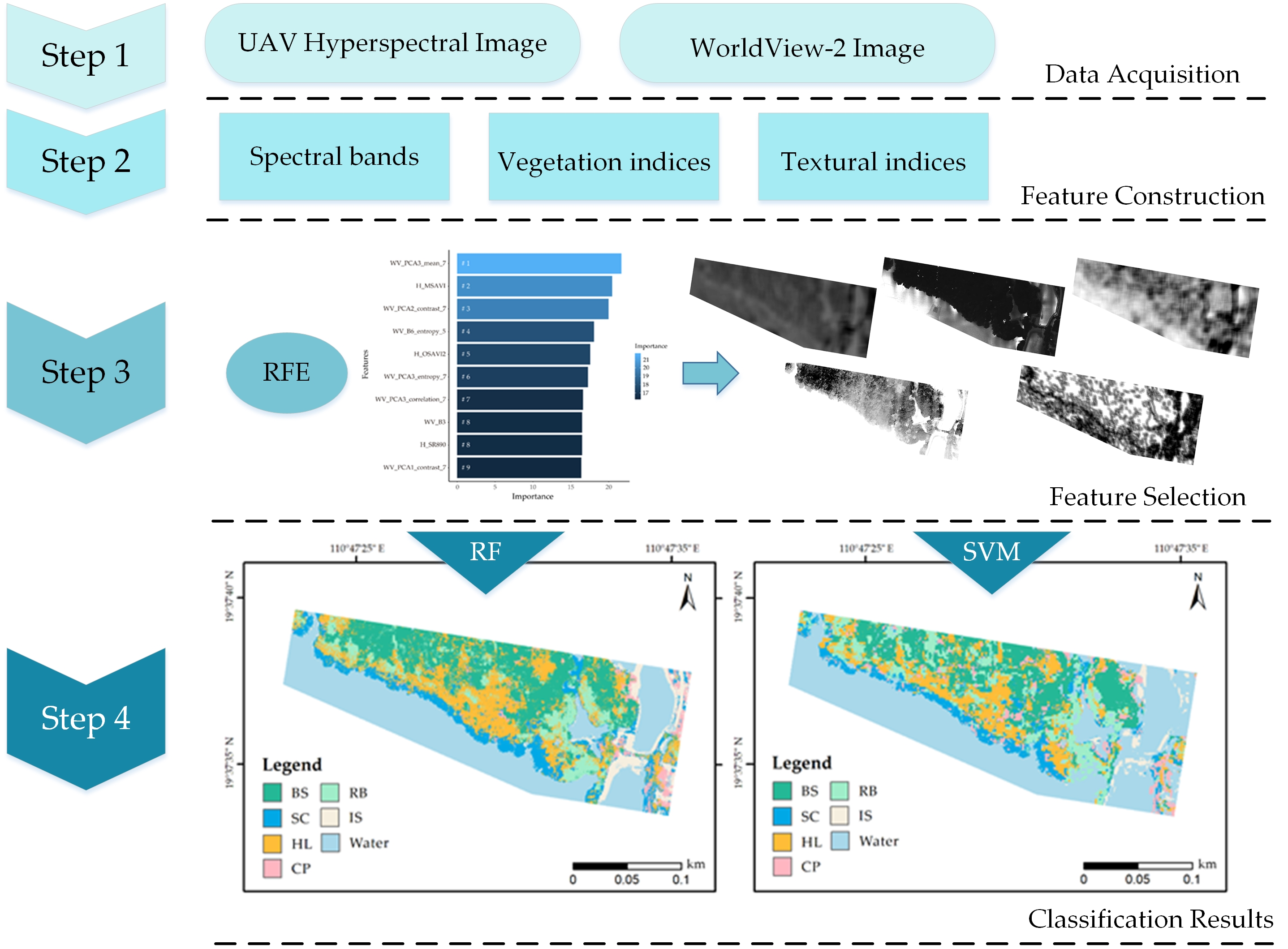
2.4. Feature Construction and Selection Method

The rich data from hyperspectral and multispectral images make it possible to classify mangrove species; however, if the raw data are not extracted and preferred, the large amount of redundant information will provoke a dimensional disaster, and thus overfitting will occur in the image classification process. Therefore, dimensionality reduction through techniques such as feature extraction and feature selection is critical. With the improvement of image spectral resolution, spectral feature extraction has become a research hotspot in the field of computer vision, and the curve features, similarity metric features, operations, and transformation methods of spectra are gradually developed. At present, there are more than 50 kinds of vegetation indices applied in vegetation classification research [47,48]. The vegetation indices are indirectly related to ecological factors such as soil and water in the environment. According to vegetation indices, we can reflect biological parameters such as the number of photosynthetic activity products, leaf area index, and primary productivity of vegetation, and the differences of biological parameters among different kinds of vegetation provide an entry point for the application of vegetation indices for species classification [49]. The texture structure is characterized by the reflectance values between image elements, which can take into account the macroscopic and microscopic structures of the images [50]. The differences in texture features between different mangrove species provide an important basis for target identification and classification, and the addition of textural information can greatly improve the classification accuracy.

Numerous studies have proven that vegetation index features and texture features are beneficial for mangrove species classification, and the performance of feature extraction determines the effectiveness of image classification [36,51]. In this study, based on the original spectral bands of unmanned aerial vehicle hyperspectral images and WV-2 images, respectively, a series of processing steps was conducted: (1) Thirty-eight vegetation indices were extracted by a mathematical transformation method, as shown in

Table A1. Vegetation index extracted for classification.

Index	Abbreviation	Formula	Reference
By WV-2 Image
Atmospherically Resistant Vegetation Index 2	ARVI2	$-0.18+1.17\times \left(\frac{R_{Nir}-R_{Red}}{R_{Nir}+R_{Red}}\right)$	[64]
Blue-wide Dynamic Range Vegetation Index	BWDRVI	$\frac{0.1R_{Nir}-R_{Blue}}{0.1R_{Nir}+R_{Blue}}$	[65]
Canopy Chlorophyll Content Index	CCCI	$\frac{R_{Nir}-R_{Rededge}}{R_{Nir}+R_{Rededge}}/\frac{R_{Nir}-R_{Red}}{R_{Nir}+R_{Red}}$	[66]
Corrected Transformed Vegetation Index	CTVI	$\frac{NDVI+0.5}{\left|NDVI+0.5\right|}\sqrt{\left|\left(NDVI\right)+0.5\right|}$	[67]
Chlorophyll vegetation index	CVI	$R_{Nir}\times \frac{R_{Red}}{R_{Green}{}^2}$	[68]
Differenced Vegetation Index 75	DVI75	$R_{Nir}-R_{Red}$	[69]
Differenced Vegetation Index 85	DVI85	$R_{Nir\_B8}-R_{Red}$	[69]
Differenced Vegetation Index 73	DVI73	$R_{Nir}-R_{Green}$	[70]
Enhanced Vegetation Index	EVI	$2.5\frac{R_{Nir}-R_{Red}}{R_{Nir}+6R_{Red}-7.5R_{Blue}+1}$	[71]
Enhanced Vegetation Index 2	EVI2	$2.5\frac{R_{Nir}-R_{Red}}{R_{Nir}+2.4R_{Red}+1}$	[72]
Green atmospherically resistant vegetation index	GARI	$\frac{R_{Nir}-\left(R_{Green}-\left(R_{Blue}-R_{Red}\right)\right)}{R_{Nir}-\left(R_{Green}+\left(R_{Blue}-R_{Red}\right)\right)}$	[73]
Global Environment Monitoring Index	GEMI	$n\left(1-0.25n\right)\times \frac{R_{Red}-0.125}{1-R_{Red}}$ $\mathrm{n}=\frac{\left(2\right(R_{Nir}{}^2-R_{Red}{}^2)+1.5R_{Nir}+0.5R_{Red})}{R_{Nir}+R_{Red}+0.5}$	[48]
Ideal vegetation index	IVI	$\frac{R_{Nir}-b}{a\times R_{Red}}$	[74]
Log Ratio	LogR	$\log \left(\frac{R_{Nir}}{R_{Red}}\right)$	[75]
Normalized Difference Vegetation Index 75	NDVI75	$\frac{R_{Nir}-R_{Red}}{R_{Nir}+R_{Red}}$	[76]
Normalized Difference Vegetation Index 85	NDVI85	$\frac{R_{Nir2}-R_{Red}}{R_{Nir2}+R_{Red}}$	[76]
Normalized Difference Vegetation Index 86	NDVI86	$\frac{R_{Nir2}-R_{Rededge}}{R_{Nir2}+R_{Rededge}}$	[77]
Normalized Difference Vegetation Index 83	NDVI83	$\frac{R_{Nir2}-R_{Green}}{R_{Nir2}+R_{Green}}$	[78]
Normalized Difference Water Index 37	NDWI37	$\frac{R_{Green}-R_{Nir}}{R_{Green}+R_{Nir}}$	[79]
Normalized Difference Water Index 38	NDWI38	$\frac{R_{Green}-R_{Nir2}}{R_{Green}+R_{Nir2}}$	[79]
Simple Ratio 75	SR75	$R_{Nir}/R_{Red}$	[80]
Simple Ratio 85	SR85	$R_{Nir2}/R_{Red}$	[79]
Transformed Soil Adjusted Vegetation Index	TSAVI	$\frac{s\left(R_{Nir}-s\times R_{Red}-a\right)}{a\times R_{Nir}+R_{Red}-a\times s+X\left(1+s^2\right)}$	[81,82,83]
By UAV Hyperspectral Image
Bow Curvature Reflectance Index	BCRI	$\frac{R_{550}+R_{650}}{2}-R_{670}$	[84]
Carotenoid Reflectance Index 1	CRI1	$\frac{1}{R_{510}}-\frac{1}{R_{550}}$	[85]
Carotenoid Reflectance Index 2	CRI2	$\frac{1}{R_{510}}-\frac{1}{R_{700}}$	[85]
Gitelson2	Gitelson2	$\left(R_{750}+R_{800}/R_{695}+R_{740}\right)-1$	[86]
Modified Soil Adjusted Vegetation Index	MSAVI	$0.5\left(2R_{800}+1-\sqrt{{\left(2R_{800}+1\right)}^2-8\left(R_{800}-R_{670}\right)}\right)$	[87,88]
Normalized Difference Vegetation Index 750	NDVI750	$\frac{R_{750}-R_{705}}{R_{750}+R_{705}}$	[77]
Normalized Difference Vegetation Index 800	NDVI800	$\frac{R_{Nir}+R_{Red}}{R_{Nir}+R_{Red}}$	[76]
Optimized Soil Adjusted Vegetation Index 2	OSAVI2	$\left(1+0.16\right)\times \left(R_{750}+R_{705}\right)/\left(R_{750}+R_{705}+0.16\right)$	[89]
Renormalized Difference Vegetation Index	RDVI	$\frac{R_{800}+R_{670}}{\sqrt{\left(R_{800}+R_{670}\right)}}$	[90]
Red Edge Position Index	REP	$695+45\left(\frac{R_{Re}+R_{695}}{R_{740}+R_{695}}\right)$	[91]
Reflectance at the inflexion point	Rre	$\left(R_{665}+R_{786}\right)/2$	[91]
Red‒Green Ratio Index	RG	$R_{710}/R_{540}$	[92]
Photochemical Reflectance Index	PRI	$\frac{R_{531}-R_{570}}{R_{531}+R_{570}}$	[93]
Simple Ratio 750	SR750	$R_{750}/R_{700}$	[94]
Simple Ratio 890	SR890	$R_{Nir}/R_{Red}$	[80]

s = the soil line slope; a = the soil line intercept; X = an adjustment factor that is set to minimize soil noise.

, which enhanced the vegetation information and amplified the differences between vegetation classes. (2) Eight texture measures for each band were calculated using a gray level concurrence matrix (GLCM), including mean, variance, homogeneity, angular second moment (SM), contrast, dissimilarity, entropy, and correlation, as shown in

Table A2. Textural features extracted for classification.

Textural Features	Formulation	Reference
Mean	${\mu }_i={\displaystyle {\displaystyle \sum }_i}{\displaystyle {\displaystyle \sum }_j}iP\left[i,j\right]$	[36]
Variance	${\displaystyle {\displaystyle \sum }_i}{\displaystyle {\displaystyle \sum }_j}{\left(i-{\mu }_i\right)}^{2}P\left[i,j\right]$	[95]
Homogeneity	${\displaystyle {\displaystyle \sum }_i}{\displaystyle {\displaystyle \sum }_j}\frac{P\left[i,j\right]}{1+\left|i-j\right|}$	[36]
Angular Second Moment	${\displaystyle {\displaystyle \sum }_i}{\displaystyle {\displaystyle \sum }_j}P{\left[i,j\right]}^2$	[51]
Contrast	${\displaystyle {\displaystyle \sum }_i}{\displaystyle {\displaystyle \sum }_j}{\left(i-j\right)}^{2}P\left[i,j\right]$	[51]
Dissimilarity	${\displaystyle {\displaystyle \sum }_i}{\displaystyle {\displaystyle \sum }_j}P\left[i,j\right]$	[51]
Entropy	${\displaystyle {\displaystyle \sum }_i}{\displaystyle {\displaystyle \sum }_j}P\left[i,j\right]\ln P\left[i,j\right]$	[96]
Correlation	$\frac{{{\displaystyle \sum }}_i{{\displaystyle \sum }}_{j}ijP\left[i,j\right]-{\mu }_i{\mu }_j}{{\sigma }_i{\sigma }_j}$	[96]

Notes: i is the row number of the image; j is the column number of the image; P[i,j] represents the relative frequency of two neighboring pixels. ${\mu }_i={\displaystyle \sum }_i{\displaystyle \sum }_{j}iP\left[i,j\right]·$ ${\mu }_j={\displaystyle \sum }_i{\displaystyle \sum }_{j}jP\left[i,j\right]·$ ${\sigma }_i$ and ${\sigma }_j$ are the standard deviation of values for i and j references, respectively.

, where the moving windows are 3 × 3, 5 × 5, and 7 × 7, the moving step is 1, and the moving direction is 0°. (3) A principal component analysis was performed on the image, the first three components with more than 90% of the information were extracted, and eight texture measures were extracted for each component. Together with the spectral reflectance features of the image bands, a total of 799 hyperspectral image features and 153 WV-2 image features were finally extracted, as shown in

Table 3. Object features extracted for classification *.

Object Features	UAV Hyperspectral Image	WV-2 Image
Spectral bands	45 Spectral bands	8 Spectral bands
	The first three bands obtained by PCA	The first three bands obtained by PCA
Vegetation indices	BCRI, CRI1, CRI2, Gitelson2, MSAVI, NDVI750, NDVI800, OSAVI2, PRI, RDVI, REP, RG, Rre, SR750, SR890	ARVI2, BWDRVI, CCCI, CTVI, CVI, DVI75, DVI85, DVI73, EVI, EVI2, GARI, GEMI, IVI, LogR, NDVI75, NDVI85, NDVI83, NDVI86, NDWI37, NDWI38, SR75, SR85, TSAVI
Textural index	contrast, correlation, dissimilarity, entropy, homogeneity, mean, sm, variance	contrast, correlation, dissimilarity, entropy, homogeneity, mean, sm, variance

* See Appendix A for detailed definitions.

.

For feature preference, this study first eliminated features with correlations greater than 85%, and then implemented recursive feature elimination in a random forest algorithm (RFE-RF) to initialize the set of desired features to the entire dataset, and performed backward sequential selection from the full set, eliminating one feature at a time with the lowest ranking criterion score until a subset of features that are most important for the classification is formed, which can effectively improve the stability of variable selection [52].

2.5. Classification and Validation

A pixel-based mangrove species classification and accuracy comparison uses UAV hyperspectral images, WV-2 multispectral images, and fusion images of both. Based on the RFE-RF algorithm for feature selection and determination of five features and the algorithms of random forest (RF) and support vector machine (SVM), which are accurate and efficient in the field of mangrove species classification, we classified and tuned the model parameters. To determine the stability of the classification model, 70% of the samples were randomly selected as training data and 30% as validation data. The overall accuracy, Kappa, and confusion matrix were used to estimate the accuracy of the classification results.

2.5.1. Random Forest Classifier

The RF algorithm, proposed by Breiman et al. in 2001 [53], is a classifier consisting of multiple independent decision trees for category prediction of randomly selected sample information. In constructing decision trees, data are extracted from the training sample set by the bootstrap sampling method, and each decision tree is composed of numerous binary trees, which are recursively split from the root node to bifurcate the training sample set according to the principle of minimum node purity [54]. Each decision tree is a classifier; numerous independent decision trees integrate the RF algorithm model and the random forest votes on the classification result of each decision tree to decide the final classification result. The RF algorithm has the advantages of being insensitive to parameters, being less prone to overfitting, fast training, and performing well on interspecies classification problems.

The parameters that need to be modified in the classification modeling process of the random forest algorithm are mtry (number of variables randomly sampled as candidates at each split) and ntree (number of trees to grow). To reduce the chance due to single division of the training and validation sets and to improve the generalization ability, we used a 10-fold cross-validation method, randomly partitioning the original sample into 10 equal size subsamples. Of the 10 subsamples, a single subsample is retained as the validation data for testing the model, and the remaining 9 subsamples are used as training data; the cross-validation process is then repeated 10 times. The whole process is implemented through the Caret package (https://topepo.github.io/caret/, accessed on 12 December 2020) of R/RStudio. In this study, the optimal ntree is 500 and mtry is 1 using the grid search method (https://machinelearningmastery.com/tune-machine-learning-algorithms-in-r/, accessed on 12 December 2020).

2.5.2. Support Vector Machine Classifier

Support vector machine (SVM) is a binary classification model based on statistical learning theory, which was submitted by Vapnik et al. (1964) and received widespread attention in the 1990s [55]. The learning strategy of the SVM algorithm is to find the optimal hyperplane in the feature space, minimizing the intraclass interval and maximizing the interclass interval, which can be formally understood as solving a linearly constrained convex quadratic programming problem [56]. With the escalation of user requirements, SVM has been gradually extended from applying only to binary classification problems to multiclassification aspects. One of the more common methods is to construct multiple binary classifiers and combine them in some way to achieve multiclass classification [24]. This algorithm has been widely used in hyperspectral fields due to its strong robustness and outstanding generalization ability in the processing of high-dimensional data.

The main parameters that need to be modified by the support vector machine algorithm in the classification modeling process are the kernel function, cost (regularization parameter of the error term), and gamma (handling nonlinear classification hyperparameter). Based on research experience and preliminary experimental results, it is known that the radial basis function (RBF) has the highest accuracy when applied to mangrove studies [57], so in this study the most generalized form of the SVM algorithm, RBF, is used. By calling the tune function (https://www.rdocumentation.org/packages/e1071/versions/1.7-5/topics/tune, accessed on 13 December 2020) in the e1071 package in the R/RStudio project, the optimal cost and gamma of RBF are 64 and 1, respectively, obtained in parallel and efficiently using the grid search method.

2.5.3. Accuracy Assessment

The verification samples were elected based on the distribution map of tree species distribution blocks in the field survey in 2019. To balance the influence of the accuracy component of each category on the overall accuracy, 1800 sample points were selected according to the area ratio of each class; 70% were randomly selected for classifier modeling, and 30% were randomly selected for independent accuracy verification. Due to the complicated terrain and inaccessible factors in the northeast of the study area, the distribution uniformity of samples was inadequate, but the existing samples covered all the dominant tree species in the study area. By calculating the overall accuracy, Kappa coefficient, and confusion matrix of the fine classification results of mangrove tree species, we carried out a parallel precision evaluation and analysis.

As the point selection of the traditional precision verification method is based on visual interpretation, there will be confusion between the single wood edge and the mixed area of the tree species with similar characteristics. To ensure the accuracy of classification results, 73 GPS waypoints collected on 27 December 2019 and 23 October 2020 were also used for independent validation in this study, and the confusion matrix method was adopted to improve the accuracy of the evaluation.

3. Results and Discussion

3.1. Feature Selection and Applicability Analysis

The 952 feature sets, consisting of UAV hyperspectral images and WV-2 images, were created using the RFE-RF method. After several iterations, as shown in Figure 2, when the number of variables is five, the overall accuracy reaches 95.47% and the kappa is 0.94; the classification accuracy is improved by 6.36% compared with when there are four variables. Considering that the redundancy of features causes problems with accuracy degradation and overfitting, the five most important features in the set are selected to form the feature model for classification.

The 10 variables with the greatest power in the classification were identified by the statistical feature importance index, as shown in Figure 3, where the top five selected features were WV_PCA3_mean_7, H_MSAVI, WV_PCA2_contrast_7, WV_B6_entropy_5, and H_OSAVI2. Texture features, vegetation indices, and spectral bands all performed well in the specific classification of mangroves. In general, texture features were more important than vegetation indices and spectral bands. The most important feature (WV_PCA3_mean_7) was obtained by performing a principal component analysis based on the WV-2 images and extracting the mean texture operator for the third principal component, with a 7 × 7 moving window. The most important vegetation index is the modified soil adjusted vegetation index (MSAVI).

Correlations were estimated based on the 10 features that were preferentially selected, as shown in Figure 4. All features had correlations lower than 70%, and the correlations of the top five features selected for this study were lower than 50%. The low autocorrelation property between features ensures that information is not duplicated and can effectively avoid the overfitting phenomenon. In general, most of the features extracted from different images have a negative or no correlation with each other, while most of the features extracted from the same data sources have a positive correlation.

When comparing the contributions of the two data sources to mangrove species classification, we found that only vegetation indices performed well among the features extracted from the UAV hyperspectral imagery, while the WV-2 satellite-based image data, in contrast, had better performance in texture features and spectral band features. More textural features were extracted in the study, but the contribution was relatively small, which caused serious redundancy and reduced the efficiency of feature preference. Among the eight texture feature operators, mean, dissimilarity, and entropy values can effectively improve the accuracy of mangrove interspecies classification, while contrast, correlation, homogeneity, SM, and variance had relatively poor effects. Therefore, the performance of textural features in the classification of mangrove species is decreasing with the increase of image spatial resolution and spectral resolution, while the role of vegetation index features is increasing. Overall, the use of UAV hyperspectral images and WV-2 satellite-based multispectral images, combined with vegetation index features and texture features, is beneficial to improve the classification of mangrove species.

Here, the classification accuracy and mean decrease accuracy (MDA), which represents the degree of anti-perturbation in prediction accuracy, were estimated for the seven most important features, as shown in Figure 5, and it can be seen that the classification accuracy was higher than 80% for all categories. It is worth noting that for the top five most critical features selected in this study, the importance is negatively correlated with the single-category accuracy, and the MDA is positively correlated with the single-category accuracy, indicating that, in the process of feature preference, the contribution of features to the model construction does not depend entirely on the classification accuracy, but also takes into account the degree of anti-perturbation of the classifier prediction accuracy, the impact of features on classifier impurity impact, and computational speed [58,59].

We also counted the basic spectral bands utilized for the 10 most important features and found that the red, near-infrared, red-edge, and green bands were the most used, with the narrowband channel being more useful than the wideband channel. The advantages of red and near-infrared bands for species classification are widely recognized. The red band has a longer spectral range compared to other visible bands and therefore can reflect differences among vegetation species more intuitively through spectral reflectance. Some studies have pointed out that red-band spectral reflectance can also indirectly reflect the intensity of photosynthesis in leaves [60]. The near-infrared band is a sensitive indicator of moisture content, mainly controlled by the cellular structure within the leaves [61]. The green- and red-edge bands are highly correlated with chlorophyll-a (Chl-a) concentrations, and for mangroves, chlorophyll concentrations are closely related to environmental factors such as temperature, solar radiation, salinity, and water, and different mangrove species have specific tolerances to environmental factors [60]; the variability they exhibit offers the possibility of species classification of mangroves.

3.2. Accuracy Assessment

The accuracy of RF and SVM machine learning algorithms in mangrove species classification results was verified using sample points confirmed by UAV images. As shown in

Table 4. Confusion matrix for mangrove classification with combining UAV and WV-2 image samples.

RF		Overall Accuracy: 95.89%								Kappa Coefficient: 0.95
SVM		Overall Accuracy: 95.35%								Kappa Coefficient: 0.94
	SVM	BS		SC		HL		RB		CP		IS		Water		UA
RF
BS		100	100	0	0	2	2	5	2	1	0	0	0	0	0	0.93	0.96
SC		0	0	54	51	1	0	1	3	2	1	0	0	0	0	0.93	0.93
HL		0	0	0	0	101	102	6	2	0	0	0	0	0	0	0.94	0.98
RB		0	0	0	0	2	2	70	73	1	0	0	0	0	0	0.96	0.97
CP		0	0	0	3	0	0	0	2	30	31	0	0	0	0	1	0.86
IS		0	0	0	0	0	0	0	0	0	0	49	43	1	0	0.98	1.00
Water		0	0	0	0	0	0	0	0	0	2	1	7	132	133	0.99	0.94
PA		1	1	1	0.94	0.95	0.96	0.85	0.89	0.88	0.91	0.98	0.86	0.99	1

, the overall accuracy of the RF algorithm was 95.89% and the kappa coefficient was 0.95, and the overall accuracy of the SVM algorithm was 95.35% and the kappa coefficient was 0.94. Overall, the two machine learning algorithms performed well in the classification of mangrove species.

As shown in

Table 5. Confusion matrix for mangrove classification with GPS waypoints.

RF		Overall Accuracy: 91.78%								Kappa Coefficient: 0.90
SVM		Overall Accuracy: 84.93%								Kappa Coefficient: 0.82
	SVM	BS		SC		HL		RB		CP		IS		Water		UA
RF
BS		14	12	0	0	1	0	2	1	0	1	0	0	0	0	0.82	0.86
SC		0	0	7	7	0	0	0	0	0	0	0	0	0	0	1	1
HL		1	2	0	0	8	8	0	1	1	1	0	0	0	0	0.80	0.67
RB		1	2	0	0	0	1	16	16	0	0	0	0	0	0	0.94	0.84
CP		0	0	0	0	0	0	0	0	6	5	0	0	0	0	1	1
IS		0	0	0	0	0	0	0	0	0	0	6	5	0	1	1	0.83
Water		0	0	0	0	0	0	0	0	0	0	0	1	10	9	1	0.90
PA		0.88	0.75	1	1	0.89	0.89	0.89	0.89	0.86	0.71	1	0.83	1	0.90

, the overall accuracy of the RF algorithm was 91.78% and the kappa coefficient was 0.90, which was 4.11% lower than the accuracy of the sample point validation. The results of the two validation methods had high consistency, indicating that the RF algorithm has a more far-reaching application in the classification of mangrove species. As for RF, the overall accuracy was 84.93% and the kappa coefficient was 0.82, which was 10.42% lower than the sample point validation accuracy. The results of the two validation methods were very different, indicating that the SVM algorithm led to overfitting in the process of mangrove species classification.

In the field of mangrove species classification, the RF algorithm has good mapping and high classification accuracy, making it more worthwhile than the SVM algorithm. In terms of individual types of classification accuracy, as shown in Figure 6, the RF’s validation accuracy performance was stable, while the SVM accuracy for different types of classification was more variable. The accuracy of GPS waypoint validation is generally lower than that of sample points validation, which is closer to the actual situation. There are extremes in the GPS waypoint verification accuracy results, which are mainly caused by the small number of waypoints collected for some cover types. Among the four species of mangrove, SC had the best divisibility and showed a spatial location distribution pattern consistent with the fact that SC often grows at the border between mangroves and seawater. Tree species with low classification accuracy in mangroves are RB, HL, and BS, mainly because Derris trifoliata gets tangled up with the trunk and canopy of RB, HL, and BS. As a result, training samples of different mangrove species will have less information on Derris trifoliata, which confuses the training and validation samples of classification and interferes with the construction of classification models, resulting in lower classification accuracy. The canopy leaf shapes of RB and BS are similar, and the effectiveness of texture features is diminished, leading to serious misclassification on the mixed border of RB and BS leaves. In addition, factors such as differences in spectral information between new, old, and diseased leaves of mangroves can cause a reduction in the fine classification accuracy of tree species.

3.3. Comparison of Mangrove Mapping and Analysis of Drivers

To investigate the potential of UAV hyperspectral imagery in the field of mangrove species classification, this study used two machine learning algorithms, RF and SVM, to investigate the finer classification of mangroves based on integrated features, including 799 features extracted from UAV hyperspectral images and 153 features extracted from WV-2 images.

As shown in Figure 7, the accuracy of mangrove species classification using UAV hyperspectral imagery is significantly higher than that using WV-2 imagery, and the accuracy of integrated UAV hyperspectral imagery and WV-2 multispectral imagery is slightly improved compared with that of UAV hyperspectral imagery. This indicates that, in the field of fine-grained interspecies classification, the higher the spatial resolution, the higher the classification accuracy. As the resolution increases, the spatial correlation between adjacent image element values of all feature classes decreases [50], which is consistent with the findings of the image resolution on the classification accuracy of features. In 2019, Penghua Qiu used the UAV LIDAR and WorldView-2 data from the same study area of Qinglan Harbor Mangrove Reserve for species classification of mangroves with an overall accuracy of 86.08% [42], which was 9.81% lower compared to the results of this study. Different resolution optical images have great potential to be explored, and studies that simply introduce different types of remote sensing data without trying to explore the value of the data in depth are blind. In the field of mangrove species classification, the RF algorithm outperformed the SVM algorithm in terms of the accuracy performance for all three different data sources. From the independent validation results of GPS waypoints, RF is more well-built than SVM, while the two validation results of the SVM algorithm have a large gap and overfitting phenomenon, which is related to the large similarity of spectral information of mangrove tree species. As shown in Figure 6, RF has a higher balance of interspecies classification accuracy than SVM, which is more suitable for distinguishing multiple classes, while the SVM has high recognition accuracy for SC and low recognition accuracy for IS with poor model comprehensibility, which is more suitable for dichotomous classification problems. Both the RF and SVM algorithms are insensitive to the recognition of RB and CP, which is related to their large range of intraclass spectral value distribution, which is not conducive to distinguishing them from other tree species.

As shown in Figure 8, based on the combined data with the highest accuracy, the classification results of mangrove forests in the study area of Qinglan Harbor, Hainan Province, were classified using RF and SVM methods. The figure includes a total of seven land types, including Rhizophora apiculata Blume (RB), Bruguiera sexangula (BS), Hibiscus tiliaceus Linn. (HL), Sonneratia caseolaris (SC), coconut palm (CP), impervious surface (IS), and water. Comparing Figure 8a,b, we see that there are small areas of misclassification in the classification result map of the SVM method; for example, there is no CP distribution in the vegetation area in the west, and some areas of RB and BS are confused with each other. The RF method has better classification enforcement than the SVM method, which is consistent with the spatial distribution pattern of mangrove growth in the study area. In addition, we found that the RF algorithm is insensitive to parameters and the classification process is more efficient, while the SVM algorithm takes a long time and is relatively less efficient in the parameter preference process.

We also investigated the source of errors during the mangrove species classification process. (1) When using UAV to capture images, avoid direct sunlight on mangroves at noon as it generates a lot of noise and affects the overall quality of images; the best periods are generally from 8:30 to 9:30 a.m. and from 3:00 to 4:00 p.m. Affected by the angle of sunlight, some areas of the images will be covered with shadows, making the heterogeneity of the same tree species increase and the similarity of different types of tree species increase, which makes the classification work more difficult. (2) Due to differences in capture time, meteorological conditions, and spatial resolution of different data, as well as the systematic errors of sensors, there are inconsistencies in the spatial distribution of mangroves from different data sources in some areas, and although this study has been carefully screened by visual interpretation during the experiment, some sample points may still have errors corresponding to the information of multiple species. (3) In addition, when the GPS fixation survey marked mangrove species information, the local field of view was obscured and it was more difficult to obtain a real-time accurate global field of view information, which could lead to misjudging the canopy mangrove species information of some points taken vertically by remote sensing images. (4) The richness of mangrove species in the study area, the high density of mixed species, the staggering growth and distribution of different tree species, and some of the mangrove trees with high height and sparse leaves often having another species of mangrove growing underneath, which greatly reduces the purity of image pixels [62] (called the mixed pixel effect) increase the difficulty of drawing visual distinctions between tree species, as shown by the overestimation of the verification accuracy of classification results contrasted with the actual distribution.

4. Conclusions

In this study, we used UAV Rikola hyperspectral images and WV-2 satellite-based multispectral images to classify mangroves in Qinglan Harbor and investigated the feasibility and limitations of different types of high-resolution sensors for vegetation classification. The results showed that the combined data accuracy (95.89%) is higher than that of UAV (94.21%) and WV-2 (73.59%) data individually. The vegetation index features of UAV hyperspectral image and texture index of satellite-based multispectral image play a prominent role, and their source spectral bands are red, near-infrared, red-edge, and green bands. The RF algorithm was applied to the combined data with the highest accuracy (95.89%) and also outperformed the SVM algorithm in terms of stability and adaptability. Besides, it was also explored that the main causes of errors were spatial misalignment of mangroves on different spatial resolution images and the complex natural environment in the field, resulting in impure sample information that interfered with the classifier modelling.

Human overexploitation and mismanagement of mangroves are leading to a rapid decline in mangrove forests worldwide [63], and the feasibility and development potential of mangrove species classification was confirmed by using high-quality data. Additionally, based on the study of two different spatial resolution images, the object-based method could not be implemented, but its application to UAV hyperspectral images could be considered for in-depth exploration in the future.

Future research will explore new ideas for mangrove species classification, by contemplating continuously accumulating sample data, establishing a mangrove sample database, applying deep learning algorithms to the study of the fine classification, and also conducting spatial and temporal variation analysis of mangrove species to provide suggestions for the cultivation and protection of mangroves.

References

1. Pearce, D. Nature’s services: Societal dependence on natural ecosystems. Science 1997, 277, 1783–1784. [Google Scholar] [CrossRef]
2. Cummings, C.A.; Todhunter, P.E.; Rundquist, B.C. Using the Hazus-MH flood model to evaluate community relocation as a flood mitigation response to terminal lake flooding: The case of Minnewaukan, North Dakota, USA. Appl. Geogr. 2012, 32, 889–895. [Google Scholar] [CrossRef]
3. Heenkenda, M.K.; Joyce, K.E.; Maier, S.W.; de Bruin, S. Quantifying mangrove chlorophyll from high spatial resolution imagery. ISPRS J. Photogramm. 2015, 108, 234–244. [Google Scholar] [CrossRef]
4. Edward, B.B.; Sally, D.H.; Chris, K.; Evamaria, W.K.; Adrian, C.S.; Brian, R.S. The value of estuarine and coastal ecosystem services. Ecol. Monogr. 2011, 81, 169–193. [Google Scholar]
5. Donato, D.C.; Kauffman, J.B.; Murdiyarso, D.; Kurnianto, S.; Stidham, M.; Kanninen, M. Mangroves among the most carbon-rich forests in the tropics. Nat. Geosci. 2011, 4, 293–297. [Google Scholar] [CrossRef]
6. Abdel-Aziz, S.M.; Aeron, A.; Garg, N. Microbes in Food and Health, 1st ed.; Springer International Publishing: Cham, Switzerland, 2016. [Google Scholar]
7. Wang, L.; Jia, M.; Yin, D.; Tian, J. A review of remote sensing for mangrove forests: 1956–2018. Remote Sens. Environ. 2019, 231, 111223. [Google Scholar] [CrossRef]
8. Marois, D.E.; Mitsch, W.J. Coastal protection from tsunamis and cyclones provided by mangrove wetlands—A review. Int. J. Biodivers. Sci. Ecosyst. Serv. Manag. 2015, 11, 71–83. [Google Scholar] [CrossRef]
9. Alongi, D.M. The Energetics of Mangrove Forests; Springer International Publishing: Cham, Switzerland, 2009. [Google Scholar]
10. Bindu, G.; Rajan, P.; Jishnu, E.S.; Ajith, J.K. Carbon stock assessment of mangroves using remote sensing and geographic information system. Egypt. J. Remote Sens. Space Sci. 2020, 23, 1–9. [Google Scholar] [CrossRef]
11. Giri, C.; Ochieng, E.; Tieszen, L.L.; Zhu, Z.; Singh, A.; Loveland, T.; Masek, J.; Duke, N. Status and distribution of mangrove forests of the world using earth observation satellite data. Glob. Ecol. Biogeogr. 2011, 20, 154–159. [Google Scholar] [CrossRef]
12. NASA Study Maps the Roots of Global Mangrove Loss. Available online: https://climate.nasa.gov/news/3009/nasa-study-maps-the-roots-of-global-mangrove-loss/ (accessed on 18 August 2020).
13. Prakash, H.J.; Samanta, S.; Rani, C.N.; Misra, A.; Giri, S.; Pramanick, N.; Gupta, K.; Datta, M.S.; Chanda, A.; Mukhopadhyay, A.; et al. Mangrove classification using airborne hyperspectral AVIRIS-NG and comparing with other spaceborne hyperspectral and multispectral data. Egypt. J. Remote Sens. Space Sci. 2021, 24, 273–281. [Google Scholar]
14. Ivan, V.; Jennifer, L.B.; Joanna, K.Y. Mangrove Forests: One of the World’s Threatened Major Tropical Environments. BioScience 2001, 51, 807–815. [Google Scholar]
15. Daniel, A.F.; Kerrylee, R.; Catherine, E.L.; Ken, W.K.; Stuart, E.H.; Shing, Y.L.; Richard, L.; Jurgenne, P.; Anusha, R.; Suhua, S. The State of the World’s Mangrove Forests: Past, Present, and Future. Annu. Rev. Env. Resour. 2019, 44, 89–115. [Google Scholar]
16. Jordan, R.C.; Alysa, M.D.; Brenna, M.S.; Michael, K.S. Monitoring mangrove forest dynamics in Campeche, Mexico, using Landsat satellite data. Remote Sens. Appl. Soc. Environ. 2018, 9, 60–68. [Google Scholar]
17. Lorenzo, E.N.; De Jesus, B.R.J.; Jara, R.S. Assessment of mangrove forest deterioration in Zamboanga Peninsula, Philippines using LANDSAT MSS data. In Proceedings of the Thirteenth International Symposium on Remote Sensing of Environment, Environmental Research Institute of Michigan, Ann Arbor, MI, USA, 23–27 April 1979. [Google Scholar]
18. Judd, J.H.E.W. Using Remote Sensing Techniques to Distinguish and Monitor Black Mangrove (Avicennia Germinans). J. Coast. Res. 1989, 5, 737–745. [Google Scholar]
19. Holmgren, P.; Thuresson, T. Satellite remote sensing for forestry planning—A review. Scand. J. For. Res. 1998, 13, 90–110. [Google Scholar] [CrossRef]
20. Long, B.G.; Skewes, T.D. GIS and remote sensing improves mangrove mapping. In Proceedings of the 7th Australasian Remote Sensing Conference Proceedings, Melbourne, Australia, 1–4 March 1994. [Google Scholar]
21. Wang, L.; Silván-Cárdenas, J.L.; Sousa, W.P. Neural Network Classification of Mangrove Species from Multi-seasonal Ikonos Imagery. Photogramm. Eng. Remote Sens. 2008, 74, 921–927. [Google Scholar] [CrossRef]
22. Tang, H.; Liu, K.; Zhu, Y.; Wang, S.; Song, S. Mangrove community classification based on worldview-2 image and SVM method. Acta Sci. Nat. Univ. Sunyatseni 2015, 54, 102. [Google Scholar]
23. Tian, J.; Wang, L.; Li, X.; Gong, H.; Shi, C.; Zhong, R.; Liu, X. Comparison of UAV and WorldView-2 imagery for mapping leaf area index of mangrove forest. Int. J. Appl. Earth Obs. Geoinf. 2017, 61, 22–31. [Google Scholar] [CrossRef]
24. Qiaosi, L.; Frankie, K.K.W.; Tung, F. Classification of Mangrove Species Using Combined WordView-3 and LiDAR Data in Mai Po Nature Reserve, Hong Kong. Remote Sens. 2019, 11, 2114. [Google Scholar]
25. Dezhi, W.; Bo, W.; Penghua, Q.; Yanjun, S.; Qinghua, G.; Xincai, W. Artificial Mangrove Species Mapping Using Pléiades-1: An Evaluation of Pixel-Based and Object-Based Classifications with Selected Machine Learning Algorithms. Remote Sens. 2018, 10, 294. [Google Scholar]
26. Wang, M.; Cao, W.; Guan, Q.; Wu, G.; Jiang, C.; Yan, Y.; Su, X. Potential of texture metrics derived from high-resolution PLEIADES satellite data for quantifying aboveground carbon of Kandelia candel mangrove forests in Southeast China. Wetl. Ecol. Manag. 2018, 26, 789–803. [Google Scholar] [CrossRef]
27. Wang, L.; Sousa, W.P.; Gong, P.; Biging, G.S. Comparison of IKONOS and QuickBird images for mapping mangrove species on the Caribbean coast of Panama. Remote Sens. Environ. 2004, 91, 432–440. [Google Scholar] [CrossRef]
28. Neukermans, G.; Dahdouh-Guebas, F.J.G.K.; Kairo, J.G.; Koedam, N. Mangrove species and stand mapping in Gazi bay (Kenya) using quickbird satellite imagery. J. Spat. Sci. 2008, 53, 75–86. [Google Scholar] [CrossRef]
29. Wang, L.; Sousa, W.P.; Gong, P. Integration of object-based and pixel-based classification for mapping mangroves with IKONOS imagery. Int. J. Remote Sens. 2004, 25, 5655–5668. [Google Scholar] [CrossRef]
30. Mark, A.B.; Peter, S.; Roel, R.L. Long-term Changes in Plant Communities Influenced by Key Deer Herbivory. Nat. Areas J. 2006, 26, 235–243. [Google Scholar]
31. Chen, B.; Xiao, X.; Li, X.; Pan, L.; Doughty, R.; Ma, J.; Dong, J.; Qin, Y.; Zhao, B.; Wu, Z.; et al. A mangrove forest map of China in 2015: Analysis of time series Landsat 7/8 and Sentinel-1A imagery in Google Earth Engine cloud computing platform. ISPRS J. Photogramm. 2017, 131, 104–120. [Google Scholar] [CrossRef]
32. Pham, T.D.; Xia, J.; Baier, G.; Le, N.N.; Yokoya, N. Mangrove Species Mapping Using Sentinel-1 and Sentinel-2 Data in North Vietnam. In Proceedings of the IEEE International Geoscience and Remote Sensing Symposium, Yokohama, Japan, 28 July–2 August 2019. [Google Scholar]
33. Liu, C.C.; Chen, Y.Y.; Chen, C.W. Application of multi-scale remote sensing imagery to detection and hazard analysis. Nat. Hazards 2013, 65, 2241–2252. [Google Scholar] [CrossRef]
34. Bhardwaj, A.; Sam, L.; Martín-Torres, F.J.; Kumar, R. UAVs as remote sensing platform in glaciology: Present applications and future prospects. Remote Sens. Environ. 2016, 175, 196–204. [Google Scholar] [CrossRef]
35. Claudia, K.; Andrea, B.; Steffen, G.; Tuan, V.Q.; Stefan, D. Remote Sensing of Mangrove Ecosystems: A Review. Remote Sens. 2011, 3, 878–928. [Google Scholar]
36. Cao, J.; Leng, W.; Liu, K.; Liu, L.; He, Z.; Zhu, Y. Object-Based Mangrove Species Classification Using Unmanned Aerial Vehicle Hyperspectral Images and Digital Surface Models. Remote Sens. 2018, 10, 89. [Google Scholar] [CrossRef] [Green Version]
37. Dennis, C.D.; Steven, E.F.; Monique, G.D. A comparison of pixel-based and object-based image analysis with selected machine learning algorithms for the classification of agricultural landscapes using SPOT-5 HRG imagery. Remote Sens. Environ. 2012, 118, 259–272. [Google Scholar]
38. Franklin, S.E.; Ahmed, O.S.; Williams, G. Northern Conifer Forest Species Classification Using Multispectral Data Acquired from an Unmanned Aerial Vehicle. Photogramm. Eng. Remote Sens. 2017, 83, 501–507. [Google Scholar] [CrossRef]
39. Herbeck, L.S.; Krumme, U.; Andersen, T.R.J.; Jennerjahn, T.C. Decadal trends in mangrove and pond aquaculture cover on Hainan (China since 1966: Mangrove loss, fragmentation and associated biogeochemical changes. Estuar. Coast. Shelf Sci. 2018, 233, 106531. [Google Scholar] [CrossRef]
40. Yang, Z.; Xue, Y.; Su, S.; Wang, X.; Lin, Z.; Chen, H. Survey of Plant Community Characteristics in Bamenwan Mangrove of Wenchang City. J. Landsc. Res. 2018, 10, 93–96. [Google Scholar]
41. Li, M.S.; Lee, S.Y. Mangroves of China: A brief review. For. Ecol. Manag. 1997, 96, 241–259. [Google Scholar] [CrossRef]
42. Qiu, P.; Wang, D.; Zou, X.; Yang, X.; Xie, G.; Xu, S.; Zhong, Z. Finer Resolution Estimation and Mapping of Mangrove Biomass Using UAV LiDAR and WorldView-2 Data. Forests 2019, 10, 871. [Google Scholar] [CrossRef] [Green Version]
43. Liu, M.; Mao, D.; Wang, Z.; Li, L.; Man, W.; Jia, M.; Ren, C.; Zhang, Y. Rapid Invasion of Spartina alterniflora in the Coastal Zone of Mainland China: New Observations from Landsat OLI Images. Remote Sens. 2018, 10, 1933. [Google Scholar] [CrossRef] [Green Version]
44. Shridhar, D.J.; Somashekhar, S.V.; Alvarinho, J.L. A Synoptic Review on Deriving Bathymetry Information Using Remote Sensing Technologies: Models, Methods and Comparisons. Adv. Remote Sens. 2015, 4, 147. [Google Scholar]
45. Muditha, H.; Karen, J.; Stefan, M.; Renee, B. Mangrove Species Identification: Comparing WorldView-2 with Aerial Photographs. Remote Sens. 2014, 6, 6064–6088. [Google Scholar]
46. Deidda, M.; Sanna, G. Pre-processing of high resolution satellite images for sea bottom classification. Eur. J. Remote Sens. 2012, 44, 83–95. [Google Scholar] [CrossRef]
47. Ahamed, T.; Tian, L.; Zhang, Y.; Ting, K.C. A review of remote sensing methods for biomass feedstock production. Biomass Bioenergy 2011, 35, 2455–2469. [Google Scholar] [CrossRef]
48. Bannari, A.; Morin, D.; Bonn, F.; Huete, A.R. A review of vegetation indices. Remote Sens. Rev. 1995, 13, 95–120. [Google Scholar] [CrossRef]
49. Govender, M.; Chetty, K.; Bulcock, H. A review of hyperspectral remote sensing and its application in vegetation and water resource studies. Water SA 2007, 33, 145–151. [Google Scholar] [CrossRef] [Green Version]
50. Chen, D.; Stow, D.A.; Gong, P. Examining the effect of spatial resolution and texture window size on classification accuracy: An urban environment case. Int. J. Remote Sens. 2004, 25, 2177–2192. [Google Scholar] [CrossRef]
51. Wang, T.; Zhang, H.; Lin, H.; Fang, C. Textural–Spectral Feature-Based Species Classification of Mangroves in Mai Po Nature Reserve from Worldview-3 Imagery. Remote Sens. 2015, 8, 24. [Google Scholar] [CrossRef] [Green Version]
52. Darst, B.F.; Malecki, K.C.; Engelman, C.D. Using recursive feature elimination in random forest to account for correlated variables in high dimensional data. BMC Genet. 2018, 19, 1–6. [Google Scholar] [CrossRef] [PubMed] [Green Version]
53. Leo, B. Random Forests. Mach. Learn. 2001, 45, 5–32. [Google Scholar]
54. Sveinsson, J.; Joelsson, S.; Benediktsson, J.A. Random Forest Classification of Remote Sensing Data. Signal Image Process. Remote Sens. 2006, 978, 327–338. [Google Scholar]
55. Vladimir, C.; Yunqian, M. Practical selection of SVM parameters and noise estimation for SVM regression. Neural Netw. 2004, 17, 113–126. [Google Scholar]
56. Qiang, W.; Ding-Xuan, Z. SVM Soft Margin Classifiers: Linear Programming versus Quadratic Programming. Neural Comput. 2005, 17, 1160–1187. [Google Scholar]
57. Lien, T.H.P.; Lars, B. Monitoring mangrove biomass change in Vietnam using SPOT images and an object-based approach combined with machine learning algorithms. ISPRS J. Photogramm. 2017, 128, 86–97. [Google Scholar]
58. Hong, H.; Guo, X.; Hua, Y. Variable selection using Mean Decrease Accuracy and Mean Decrease Gini based on Random Forest. In Proceedings of the 2016 7th IEEE International Conference on Software Engineering and Service Science, Beijing, China, 26–28 August 2016. [Google Scholar]
59. Lee, H.; Kim, J.; Jung, S.; Kim, M.; Kim, S. Case Dependent Feature Selection using Mean Decrease Accuracy for Convective Storm Identification. In Proceedings of the 2019 International Conference on Fuzzy Theory and Its Applications, New Taipei City, Taiwan, 7–10 November 2019. [Google Scholar]
60. Flores-de-Santiago, F.; Kovacs, J.M.; Flores-Verdugo, F. Seasonal changes in leaf chlorophyll a content and morphology in a sub-tropical mangrove forest of the Mexican Pacific. Mar. Ecol. Prog. Ser. 2012, 444, 57–68. [Google Scholar] [CrossRef] [Green Version]
61. Penuelas, J.; Filella, I. Visible and near-infrared reflectance techniques for diagnosing plant physiological status. Trends Plant Sci. 1998, 3, 151–156. [Google Scholar] [CrossRef]
62. Tatem, A.J.; Lewis, H.G.; Atkinson, P.M.; Nixon, M.S. Super-resolution land cover pattern prediction using a Hopfield neural network. Remote Sens. Environ. 2002, 79, 1–14. [Google Scholar] [CrossRef] [Green Version]
63. Goldberg, L.; Lagomasino, D.; Thomas, N.; Fatoyinbo, T. Global declines in human-driven mangrove loss. Glob. Chang. Biol. 2020, 26, 5844–5855. [Google Scholar] [CrossRef]
64. Kaufman, Y.J.; Tanre, D. Atmospherically resistant vegetation index (ARVI) for EOS-MODIS. IEEE Trans. Geosci. Remote Sens. 1992, 30, 261–270. [Google Scholar] [CrossRef]
65. Hancock, D.W.; Dougherty, C.T. Relationships between Blue- and Red-based Vegetation Indices and Leaf Area and Yield of Alfalfa. Crop Sci. 2007, 47, 2547–2556. [Google Scholar] [CrossRef]
66. Barnes, E.M.; Clarke, T.R.; Richards, S.E.; Colaizzi, P.D.; Thompson, T. Coincident detection of crop water stress, nitrogen status, and canopy density using ground based multispectral data. In Proceedings of the Fifth International Conference on Precision Agriculture, Bloomington, MN, USA, 16–19 July 2000. [Google Scholar]
67. Perry, C.R.; Lautenschlager, L.F. Functional equivalence of spectral vegetation indexes. Remote Sens. Environ. 1984, 14, 169–182. [Google Scholar] [CrossRef]
68. Vincini, M.; Frazzi, E. A broad-band leaf chlorophyll estimator at the canopy scale for variable rate nitrogen fertilization. Sustaining the Millenium Development Goals. In Proceedings of the 33th International Symposium on Remote Sensing of Environment, Stresa, Italy, 4–9 May 2009. [Google Scholar]
69. Jordan, C.F. Derivation of Leaf-Area Index from Quality of Light on the Forest Floor. Ecology 1969, 50, 663–666. [Google Scholar] [CrossRef]
70. Tucker, C.J.; Elgin, J.H.; Iii, M.M.; Fan, C.J. Monitoring corn and soybean crop development with hand-held radiometer spectral data. Remote Sens. Environ. 1979, 8, 237–248. [Google Scholar] [CrossRef]
71. Huete, A.; Didan, K.; Miura, T.; Rodriguez, E.P.; Gao, X.; Ferreira, L.G. Overview of the radiometric and biophysical performance of the MODIS vegetation indices. Remote Sens. Environ. 2002, 83, 195–213. [Google Scholar] [CrossRef]
72. Jiang, Z.; Huete, A.R.; Didan, K.; Miura, T. Development of a 2-band enhanced vegetation index without a blue band. Remote Sens Environ. Remote Sens. Environ. 2008, 112, 3833–3845. [Google Scholar] [CrossRef]
73. Gitelson, A.A.; Kaufman, Y.J.; Merzlyak, M.N. Use of a green channel in remote sensing of global vegetation from EOS-MODIS. Remote Sens. Environ. 1996, 58, 289–298. [Google Scholar] [CrossRef]
74. Baret, F.; Guyot, G.; Engineer, I.O.E.A. TSAVI: A Vegetation Index Which Minimizes Soil Brightness Effects on LAI and APAR Estimation. In Proceedings of the 12th Canadian Symposium on Remote Sensing Symposium, Vancouver, BC, Canada, 10–14 July 1989; pp. 1355–1358. [Google Scholar]
75. Krishnan, P.; Alexander, J.D.; Butler, B.J.; Hummel, J.W. Reflectance Technique for Predicting Soil Organic Matter. Soil Sci. Soc. Am. J. 1980, 44, 1282–1285. [Google Scholar] [CrossRef]
76. Hope, A.S. Estimation of wheat canopy resistance using combined remotely sensed spectral reflectance and thermal observations. Remote Sens. Environ. 1988, 24, 369–383. [Google Scholar] [CrossRef]
77. Gitelson, A.; Merzlyak, M.N. Quantitative estimation of chlorophyll-a using reflectance spectra: Experiments with autumn chestnut and maple leaves. J. Photochem. Photobiol. B Biol. 1994, 22, 247–252. [Google Scholar] [CrossRef]
78. Buschmann, C.; Nagel, E. In vivo spectroscopy and internal optics of leaves as basis for remote sensing of vegetation. Int. J. Remote Sens. 1993, 14, 711–722. [Google Scholar] [CrossRef]
79. McFeeters, S.K. The use of the normalized difference water index (NDWI) in the delineation of open water features. Int. J. Remote Sens. 1996, 17, 1425–1432. [Google Scholar] [CrossRef]
80. Birth, G.S.; Mcvey, G.R. Measuring the Color of Growing Turf with a Reflectance Spectrophotometer. Agron. J. 1968, 60, 640–643. [Google Scholar] [CrossRef]
81. Baret, F.; Guyot, G. Potentials and limits of vegetation indices for LAI and APAR assessment. Remote Sens. Environ. 1991, 35, 161–173. [Google Scholar] [CrossRef]
82. Huete, A.R.; Post, D.F.; Jackson, R.D. Soil spectral effects on 4-space vegetation discrimination. Remote Sens. Environ. 1984, 15, 155–165. [Google Scholar] [CrossRef]
83. Li, S.; He, Y.; Guo, X. Exploration of Loggerhead Shrike Habitats in Grassland National Park of Canada Based on in Situ Measurements and Satellite-Derived Adjusted Transformed Soil-Adjusted Vegetation Index (ATSAVI). Remote Sens. 2013, 5, 432–453. [Google Scholar]
84. Jin, X.; Du, J.; Liu, H.; Wang, Z.; Song, K. Remote estimation of soil organic matter content in the Sanjiang Plain, Northest China: The optimal band algorithm versus the GRA-ANN model. Agric. For. Meteorol. 2016, 218, 250–260. [Google Scholar] [CrossRef]
85. Gitelson, A.A.; Merzlyak, M.N.; Zur, Y.; Stark, R.; Gritz, U. Non-destructive and remote sensing techniques for estimation of vegetation status. Pap. Nat. 2001, 273, 205–210. [Google Scholar]
86. Gitelson, A.A.; Gritz, Y.; Merzlyak, M.N. Relationships between leaf chlorophyll content and spectral reflectance and algorithms for non-destructive chlorophyll assessment in higher plant leaves. J. Plant Physiol. 2003, 160, 271–282. [Google Scholar] [CrossRef]
87. JG, Q.; Chehbouni, A.R.; Huete, A.R.; Kerr, Y.H.; Sorooshian, S. A Modified Soil Adjusted Vegetation Index. Remote Sens. Envrion. 1994, 48, 119–126. [Google Scholar]
88. Main, R.; Cho, M.A.; Mathieu, R.; Kennedy, M.M.O.; Ramoelo, A.; Koch, S. An investigation into robust spectral indices for leaf chlorophyll estimation. ISPRS J. Photogramm. Remote Sens. 2011, 66, 751–761. [Google Scholar] [CrossRef]
89. Wu, C.; Niu, Z.; Tang, Q.; Huang, W. Estimating chlorophyll content from hyperspectral vegetation indices: Modeling and validation. Agric. For. Meteorol. 2008, 148, 1230–1241. [Google Scholar] [CrossRef]
90. Roujean, J.L.; Breon, F.M. Estimating PAR absorbed by vegetation from bidirectional reflectance measurements. Remote Sens. Environ. 1995, 51, 375–384. [Google Scholar] [CrossRef]
91. Cho, M.A.; Sobhan, I.M.; Skidmore, A.K. Estimating fresh grass/herb biomass from HYMAP data using the red-edge position. Remote Sens. Model. Ecosyst. Sustain. 2006, 6289, 629805. [Google Scholar]
92. Gitelson, A.A.; Merzlyak, M.N. Remote estimation of chlorophyll content in higher plant leaves. Int. J. Remote Sens. 1997, 18, 2691–2697. [Google Scholar] [CrossRef]
93. Aparicio, N.; Viliegas, D.; Royo, C.; Casadesus, J.; Araus, J.L. Effect of sensor view angle on the assessment of agronomic traits by ground level hyper-spectral reflectance measurements in durum wheat under contrasting Mediterranean conditions. Int. J. Remote Sens. 2004, 25, 1131–1152. [Google Scholar] [CrossRef]
94. Boochs, F.; Kupfer, G.; Dockter, K.; Kühbauch, W. Shape of the red edge as vitality indicator for plants. Int. J. Remote Sens. 1990, 11, 1741–1753. [Google Scholar] [CrossRef]
95. Milosevic, M.; Jankovic, D.; Peulic, A. Thermography based breast cancer detection using texture features and minimum variance quantization. EXCLI J. 2014, 13, 1204. [Google Scholar] [PubMed]
96. Alharan, A.F.H.; Fatlawi, H.K.; Ali, N.S. A cluster-based feature selection method for image texture classification. Indones. J. Electr. Eng. Comput. Sci. 2019, 14, 1433–1442. [Google Scholar] [CrossRef]
Figure 1. Map of the study area, Hainan, and the field samples. Note: Rhizophora apiculata Blume (RB), Bruguiera sexangula (BS), Hibiscus tiliaceus Linn. (HL), Sonneratia caseolaris (SC), and impervious surface (IS).
Remotesensing 13 01529 g001
Figure 2. Relationship between classifier accuracy and the number of variables included.
Remotesensing 13 01529 g002
Figure 3. The top 10 selected features and their importance.
Remotesensing 13 01529 g003
Figure 4. Correlations between the 10 important features.
Remotesensing 13 01529 g004
Figure 5. Comparison of fine classification accuracy of the seven important features.
Remotesensing 13 01529 g005
Figure 6. Comparison of classification accuracy for different mangrove cover.
Remotesensing 13 01529 g006
Figure 7. Comparison of mangrove classification accuracy with different data and methods.
Remotesensing 13 01529 g007
Figure 8. Mangrove mapping in the study area with UAV hyperspectral images and WV-2 images based on: (a) RF model and (b) SVM model.
Remotesensing 13 01529 g008