Assessing the Effects of Spatial Scales on Regional Evapotranspiration Estimation by the SEBAL Model and Multiple Satellite Datasets: A Case Study in the Agro-Pastoral Ecotone, Northwestern China

Abstract

Evapotranspiration (ET) estimation is important for understanding energy exchanges and water cycles. Remote sensing (RS) is the main method used to obtain ET data over large scales. However, owing to surface heterogeneities and different model algorithms, ET estimated from RS products with different spatial resolutions can cause significant uncertainties, whose causes need to be thoroughly analyzed. In this study, the Surface Energy Balance Algorithm for Land (SEBAL) model was selected to explore spatial resolution influences on ET simulations. Three satellite datasets (Landsat Thematic Mapper (TM), Moderate Resolution Imaging Spectroradiometer (MODIS), and Advanced Very High-Resolution Radiometer (AVHRR)) were selected to independently estimate ET in SEBAL model to identify the influence of the spatial scale on ET estimation, and analyze the effects and causes of scale aggregation. Results indicated that: (1) the spatial distributions of ET estimated from the three satellite datasets were similar, with the MODIS-based ET having the largest uncertainty; and (2) aggregating input parameters had limited changes in the net radiation and soil heat fluxes. However, errors in the sensible heat and latent heat fluxes were relatively larger, which were caused by changes in the selection of hot and cold pixels and the NDVI and surface albedo parameters during scale aggregation. The scale errors caused by the model mechanisms were larger than those caused by the land use/cover pattern in the SEBAL model. Overall, this study highlights the impact of spatial scale on ET and provides a better understanding of the scale aggregation effect on ET estimation by RS.

1. Introduction

It has been widely recognized that many hydrological processes and energy exchanges are scale-dependent [1,2,3,4]. Scaling issues impact our ability to accurately model the exchanges of water and energy across the surface–atmosphere interface [5]. Several studies have illustrated that scale changes in hydrological models produce results that are considerably biased due to land surface spatial heterogeneities (e.g., variations in topography, land use/cover, and soil properties) [6,7,8,9]. Evapotranspiration (ET) is a key linchpin of the Earth’s hydrological cycle and energy balance system [10]. The accurate estimation of regional ET is crucial for water resources management, agricultural production, and ecosystem protection, particularly in water-scarce regions [11,12,13]. Owing to the limitations of the equipment and resource constraint, ground measurements of ET over large scales are nearly impossible. Remote sensing (RS) provides an ideal method for determining and mapping regional ET at different spatial scales [14,15,16]. However, considering the spatial heterogeneities of land surface properties, as well as the non-linear processes in the model algorithms, the spatial resolution of RS affects the accuracy of ET estimates in regional and larger scale modeling [17,18,19]. In order to improve the accuracy of the ET estimates and to correct the scale errors in ET simulations, it is critical to examine the scale effect on ET simulations from RS under heterogeneous surfaces [17,20,21,22,23].

The spatial resolution of the ET simulations based on RS is dependent on the satellite sensor type. Currently, satellite sensors with different spatial, temporal, and spectral resolutions have been widely used to estimate ET over multiple spatial scales [17,24,25]. These data can be divided into two categories: high spatial resolution with a poor temporal resolution (e.g., Advanced Spaceborne Thermal Emission and Reflection Radiometer (ASTER) (30/90 m, 16 d), Landsat 5 Thematic Mapper (TM) (30/120 m, 16 d), Landsat 7 Enhanced Thematic Mapper Plus (ETM+) (30/60 m, 16 d), Landsat 8 Operational Land Imager (OLI)/Thermal Infrared Sensor (TIRS) (30/100 m, 16 d)) and high temporal resolution with poor spatial resolution (e.g., Moderate Resolution Imaging Spectroradiometer (MODIS) (250/500/1000 m, 1–2 d), Advanced Very High-Resolution Radiometer (AVHRR) (1.1 km, 0.5–1 d), Spinning Enhanced Visible InfraRed Imager (SEVIRI) (5 km, 15/30 min)) [26,27,28]. Most satellite-based ET algorithms were initially developed at high spatial resolutions and hence require homogeneous conditions across a single pixel, whereas RS data contain mixed pixels, especially in low resolution datasets [29,30,31]. In addition, the parameters and processes that are important and predictive on a fine scale introduce uncertainty or significant error when being applied to a coarser scale [4,32,33,34,35]. Therefore, a noteworthy issue in RS is how ET estimates differ based on data from satellite sensors with different spatial resolutions.

To address such issues, several studies have assessed the effect of different satellite sensor types on ET simulations. Most of these studies have focused primarily on Landsat, ASTER, and MODIS sensors, and have reported good agreements in the spatial distribution patterns of the ET estimations [25,36]. However, studies have also indicated that there are discrepancies among the various spatial resolution data sources [17,18,25,31,36,37,38]. For example, McCabe and Wood [37] used Landsat-ETM, ASTER, and MODIS data to estimate ET and found consistency between the higher-resolution data sources (Landsat-TM and ASTER); however, the MODIS-based estimations were unable to discriminate the influence of land surface heterogeneity at a field scale, but correctly estimated the mean values. Sharma et al. [18] found that a regression model explained 91% of the variability in the Landsat-based crop evapotranspiration (ETc) data, and ~31% of the variability in the MODIS-based ETc data, which is higher than the measured ETc from the Bowen Ratio Energy Balance System. Landsat TM, with high spatial resolution (30 m) and MODIS with high temporal resolution (1–2 d) are widely used sensors that obtain local and regional ET information. AVHRR, another widely used sensor since the 1980s, has been used to estimate long-term ET but its accuracy has not been thoroughly analyzed in estimating regional ET [11,39,40].

In order to explore the effect of spatial resolution on ET estimation, until now, various studies have discussed the effect of the spatial resolution of input satellite data on ET estimation by a number of ET models, including the Surface Energy Balance System (SEBS) developed by Su [41] ([18,30,37]); Surface Energy Balance Algorithm for Land (SEBAL) developed by Bastiaanssen et al. [42] ([17,20,21,25,34,36]); Mapping Evapotranspiration at High Resolution with Internalized Calibration (METRIC) developed by Allen et al. [43] ([27]); Two Source Energy Balance (TSEB) developed by Norman et al. [44] ([38,45]), and Simplified Surface Energy Balance Index (S-SEBI) developed by Roerink et al. [46] ([47]), among others. These studies have pointed out that for a given area, a decrease in the number of pixels led to a loss of information, which changes the statistical and spatial characteristics of the data during the aggregation process. They have also reported that aggregation strategies, land surfaces and model mechanisms can produce different errors for ET estimation. Moreover, the aggregation of the sensible heat fluxes could cause significant errors over a heterogeneous area in the energy balance-based model. In addition, several studies have attempted to identify the reasons for the significant errors in the aggregated results. Ershadi et al. [30] and Sharma et al. [18] postulated that the aggregation processes in ET simulations may be caused by decreases in aerodynamic resistance in the energy balance model. However, Wang et al. [31] argued that, although aerodynamic resistance was excluded from the three-temperature (3T) model, due to surface heterogeneity, the spatial scale effect was still present. Ramírez-Cuesta et al. [27] indicated that surface roughness parameters and land use characteristics were the two main causes of the aggregation effect in the METRIC model. Despite these studies, in general, the aggregation effect and its causes for ET estimation remain unclear and require further study [31]. Therefore, it is necessary to comprehensively examine the changes in aggregation errors and clarify the causes of such errors in the aggregation process.

The SEBAL model, with a relatively high simulation accuracy and minimal ground-based data, is one of the most widely applied models for ET estimation [42,48]. Most of the input parameters used (e.g., Normalized Difference Vegetation Index (NDVI), land surface temperature, albedo, emissivity, and roughness length) in the SEBAL model to simulate ET are derived from raw satellite data with different spatial, spectral, and radiometric resolutions. It is therefore necessary to identify and evaluate the performance of the SEBAL model for different satellite datasets with various spatial resolutions.

In this study, the Landsat TM, MODIS, and AVHRR images and the SEBAL model were selected to analyze the effects of spatial resolution on ET estimations. The specific objectives were: (1) assessing the consistency of the SEBAL model in estimating ET using different satellite datasets; (2) quantifying the aggregation errors in the SEBAL model, and (3) identifying the main factors for scale aggregation errors. The findings of this study can provide insights for reducing scaling errors and in turn improving the accuracy of ET estimates over regional scales.

2. Materials and Methods

2.1. Study Area

The Yuyang District is located at 37.81°–38.92° N, 108.94°–110.41° E (Figure 1), Shaanxi Province, China, and covers a total area of ~7000 km². This area is part of the ecologically fragile transition zone between the desert-grassland area and the Loess Plateau region [13,49,50,51,52]. The region has a semi-arid continental monsoon climate, with an average annual temperature of 8.4 °C and an average annual precipitation of 402 mm that gradually decreases from the southeast to northwest. Approximately half of the annual precipitation occurs from July to September [53]. The altitude varies from 836 m to 1385 m above sea level, with an average of 1183 m. The main soil types are steppe aeolian sandy soil in the western part of the region, and Loess soil in the eastern part. The main land cover types (Figure 1b) are grassland (43.1%); barren land (30.6%); farmland (20.9%); wood land (3.93%); built-up land (0.85%); and water body (0.62%).

2.2. Datasets and Processing

The input data in the SEBAL model include meteorological data, satellite images, and digital elevation model (DEM) data. The satellite images were selected with less than 5% cloud coverage. Furthermore, because the in situ flux data used for model validation were measured in 2011, we chose the satellite overpass time on August 7, 2011. These data were processed using a unified projection coordinate system in the WGS-1984 coordinate system (zone M 49).

2.2.1. Remote Sensing Datasets

Landsat TM data were downloaded from the Geospatial Data Cloud website, of the Chinese Academy of Sciences (http://www.gscloud.cn, accessed on 20 May 2019). The imagery covering the study area is composed of two TM images (path 127, rows 33 and 34) on 7 August 2011. These data were corrected with a level 1 T (terrain corrected). Pre-processing of the data was mainly performed in ENVI 5.3 (ESRI). The digital number values were converted to radiance using radiation calibration, and the Fast Line-of-Sight Atmospheric Analysis of Spectral Hypercubes (FLAASH) atmospheric correction was utilized to eliminate the effects of atmosphere and light on ground reflections [54].

MODIS data were retrieved from the Land Processes Distributed Active Archive Center (LP DAAC) (https://lpdaac.usgs.gov/, accessed on 10 July 2019), including MOD09GA and MOD11A1, which include surface reflectance at a 500 m spatial resolution and surface temperature at a 1 km spatial resolution. The original MODIS products were in HDF-EOS format and sinusoidal projection, and MODIS Reprojection Tools (MRT) was used for projection transformation, format conversion, and re-sampling to convert the data into the GeoTiff format. The input data were further processed by clipping and raster calculation using the ArcGIS 10.2 (ESRI) software package to be compatible with the SEBAL model requirements.

AVHRR data were obtained from the United States National Oceanic and Atmospheric Administration Satellite Active Archive (https://www.avl.class.noaa.gov/saa/products/welcome, accessed on 23 July 2019) in high-resolution picture transmission format, with a spatial resolution of 1.1 km, and five bands (as shown in

Table 1. Wavelength of different satellite sensors.

Band Name	Wavelength (µm)
	Landsat TM	MODIS	AVHRR
Blue	0.45–0.52	0.459–0.470	0.55–0.68
Green	0.52–0.60	0.545–0.560
Red	0.63–0.69	0.630–0.690
Near infrared	0.76–0.90	0.841–0.870	0.75–1.00
Shortwave infrared 1	1.55–1.75	1.550–1.750	1.58–1.64
Shortwave infrared 2	2.08–2.35	2.105–2.115	3.55–3.93
Thermal infrared	10.40–12.50	3.66–14.385 (16 thermal infrared bands)	10.5–11.3 11.5–12.5

). The first two bands (0.55–0.68 µm and 0.75–1.00 µm, respectively) are visible light and near-infrared, which are mainly used to calculate NDVI, surface albedo, and other related coefficients. The other three bands are thermal infrared and were used to estimate land surface temperatures [55]. The data processing in this study includes radiation corrections, geometric corrections, and clipping in the ENVI 5.3 (ESRI) software package.

2.2.2. Meteorological and Flux Data

Meteorological data, including daily air temperatures (T_a) and wind speeds (U), were used as forcing data for the SEBAL model. Data from eight meteorological stations (Etuoke, Hengshan, Jingbian, Shenmu, Xingxian, Yulin, Suide, YLEOS) in the study area collected on 7 August 2011 (Figure 1a), were downloaded from Chinese National Meteorological Information Center (https://data.cma.cn/, accessed on 7 May 2019). These data were interpolated using inverse distance weighting methods to obtain their spatial distributions for the study area.

Flux data were obtained from the YLEOS (38°26′43.6″ N, 109°28′2.7″ E, 1233 m elevation). A detailed description and introduction to these data can be found in Gong et al. [53].

2.2.3. Other Data

As a model input parameter, DEM data were obtained from the Geospatial Data Cloud site, of the Chinese Academy of Sciences (http://www.gscloud.cn, accessed on 3 June 2019). The original spatial resolution of the DEM is 30 m, to match the spatial resolution of the satellite data, the nearest neighbor method is used to resample the data to 500 m and 1000 m, respectively, for the SEBAL model input. Land use/cover data were used to specify the surface roughness parameter [48] and to assist in the selection of hot and cold pixels. We utilized a 2010 land-use map with a 30 m spatial resolution, from the Resource and Environment Cloud Platform, Chinese Academy of Sciences (http://www.resdc.cn/, accessed on 20 June 2019).

2.3. Methods

2.3.1. SEBAL Model

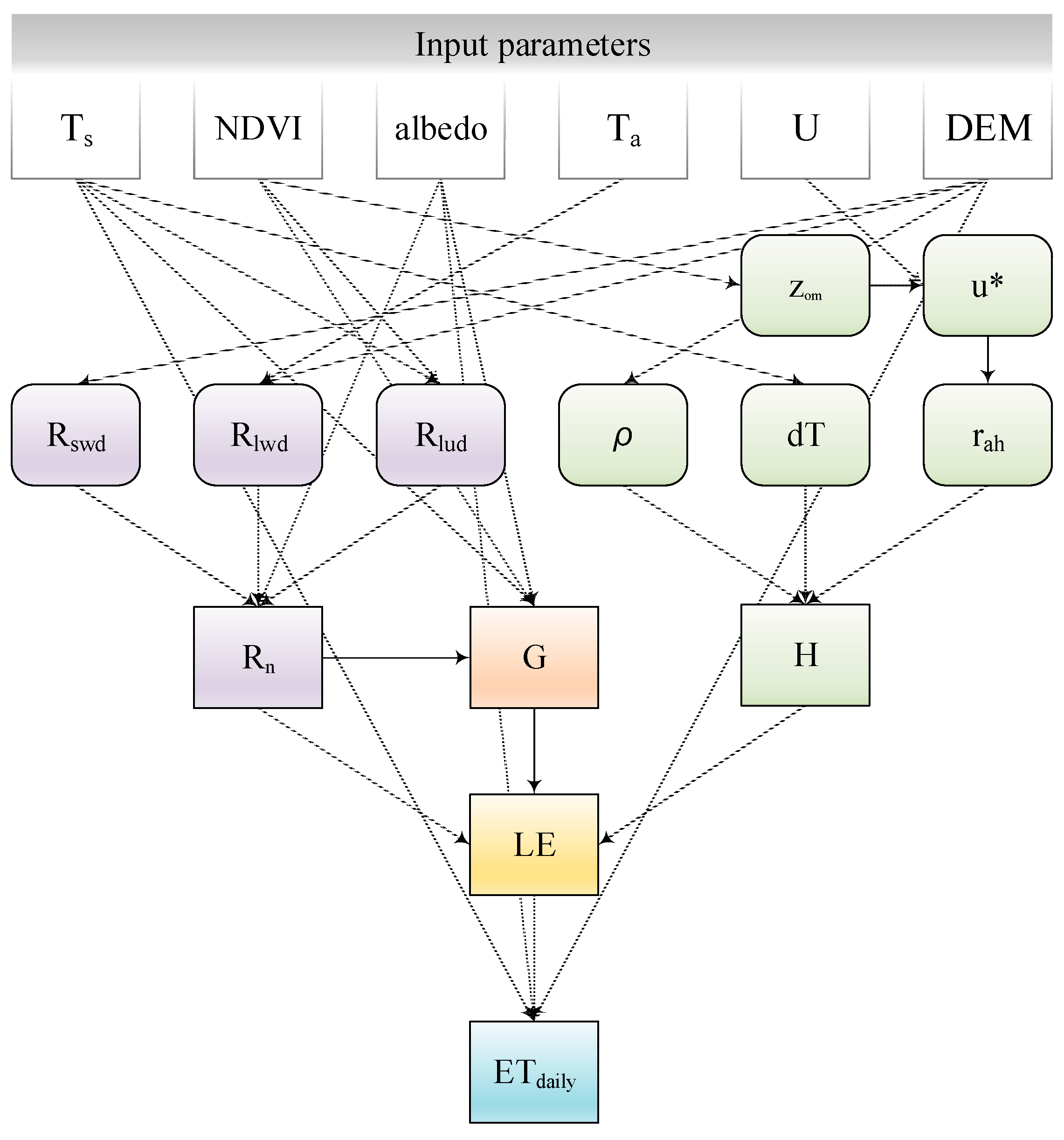
The SEBAL model was developed based on the surface energy balance equation [42]. A detailed description of the model can be found in Bastiaanssen et al. [42,48,56] and Allen et al. [57]. A flowchart for the SEBAL model algorithms is shown in Figure 2.

The energy balance equation can be expressed as follows:

$${\mathrm{R}}_{\mathrm{n}}=\mathrm{G}+\mathrm{H}+\mathrm{LE}$$

(1)

where R_n is the net radiation flux, G is the soil heat flux, H is the sensible heat flux, and LE is the latent heat flux. All units are in W/m².

The pixel-by-pixel net radiant flux calculation was obtained by subtracting the outgoing radiant components from the incoming ones [42,58]:

$${\mathrm{R}}_{\mathrm{n}}=\left(1-\mathsf{\alpha }\right){\mathrm{R}}_{\mathrm{swd}}+{\mathrm{R}}_{\mathrm{lwd}}-{\mathrm{R}}_{\mathrm{lud}}-\left(1-{\mathsf{\epsilon }}_{\mathrm{g}}\right){\mathrm{R}}_{\mathrm{lwd}}$$

(2)

where R_swd is incoming (downward) shortwave radiation (W/m²), α is the surface albedo (dimensionless), R_lwd is downward longwave radiation (W/m²), R_lud is outgoing (upward) longwave radiation (W/m²), and ε_g is the surface thermal emissivity (dimensionless).

G represents the rate of heat storage in the soil, plant, and water in heat transfer, is relatively difficult to estimate directly based on satellite data, and it can be calculated from the empirical relationship between R_n, land surface temperature, NDVI, and surface albedo, as follows [42,59]:

$$\mathrm{G}={\mathrm{R}}_{\mathrm{n}}\times \frac{1}{\mathsf{\alpha }}\times \left({\mathrm{T}}_{\mathrm{s}}-273.15\right)\times \left(0.0032\mathsf{\alpha }+0.0064{\mathsf{\alpha }}^2\right)\times \left(1-0.978{\mathrm{NDVI}}^4\right)$$

(3)

where T_s is the land surface temperature (K).

H is considered proportional to the ratio between the surface–air temperature difference (dT) and bulk aerodynamic resistance to heat transport (r_ah) [42], and it is obtained from Equation (4):

$$\mathrm{H}=\frac{{\mathsf{\rho }\mathrm{C}}_{\mathrm{p}}\mathrm{dT}}{{\mathrm{r}}_{\mathrm{ah}}}={\mathsf{\rho }\mathrm{C}}_{\mathrm{p}}\left({\mathrm{aT}}_{\mathrm{s}}+\mathrm{b}\right)/{\mathrm{r}}_{\mathrm{ah}}$$

(4)

where $\mathsf{\rho }$ is the air density (kg/m³), C_p is the air specific heat at a constant pressure (1004 J/kg/K); dT is the temperature difference between heights z₁ and z₂ (K); z₁, specified as 0.01 m, is the height above the zero-plane displacement height of the crop canopy; z₂, as 2 m, is the distance above the zero-plane displacement, but below the height of the surface boundary layer.

Due to the two unknown variables (dT and r_ah) in the equation, in this algorithm, two anchor pixels (referred to as hot and cold pixels) were chosen based on their land surface temperatures, and then the variables of dT and r_ah were calculated using a trial-and-error method in an iterative process. The cold pixels were selected from areas with an adequate water supply and lush vegetation and fully irrigated area (high NDVI, low temperature value and low albedo), and sensible heat flux is negligible, $\mathrm{LE}\approx {\mathrm{R}}_{\mathrm{n}}-\mathrm{G}$. Hot pixels were selected from sparsely vegetated and desert areas (high temperature, high albedo and low NDVI), and the latent heat flux is negligible, $\mathrm{H}\approx {\mathrm{R}}_{\mathrm{n}}-\mathrm{G}$. Bastiaanssen et al. [48] suggested that the cold pixels can be identified in open water bodies or in well-irrigated agricultural fields, and that the hot pixels can be chosen in bare soil surface. In this study, for each image, the specific extreme pixel selection was based on the land-use map, albedo, T_s, and NDVI.

r_ah is dependent on surface roughness, wind speed, and atmospheric stability [60]. It is calculated as

$${\mathrm{r}}_{\mathrm{ah}}=\frac{\ln \left(\frac{{\mathrm{z}}_2}{{\mathrm{z}}_1}\right)}{\mathrm{k}\times {\mathrm{u}}^{*}}$$

(5)

$${\mathrm{u}}^{*}=\frac{\mathrm{k}\times {\mathrm{U}}_{\mathrm{x}}}{\ln \left(\frac{{\mathrm{z}}_{\mathrm{x}}}{{\mathrm{z}}_{\mathrm{om}}}\right)}$$

(6)

where k is the von Karman’s constant (0.41), U_x is the wind speed (m/s) at height z_x, u* is the friction velocity (m/s), and ${\mathrm{z}}_{\mathrm{om}}$ is the momentum roughness length for each pixel (m), which can be calculated as Equation (7) [61]:

$${\mathrm{z}}_{\mathrm{om}}=0.05+0.5/{\left(\frac{\mathrm{NDVI}}{{\mathrm{NDVI}}_{\max }}\right)}^{2.5}$$

(7)

The LE is the residual of the energy balance equation (Equation (1)).

The evaporative fraction (EF), defined as the ratio of LE and the available radiant energy, has been shown to be approximately constant during the daytime [62,63]. The EF can be calculated as:

$$\mathrm{EF}=\frac{\mathrm{LE}}{{\mathrm{R}}_{\mathrm{n}}-\mathrm{G}}=\frac{{\mathrm{R}}_{\mathrm{n}}-\mathrm{G}-\mathrm{H}}{{\mathrm{R}}_{\mathrm{n}}-\mathrm{G}}$$

(8)

Then, the instantaneous ET (ET_inst) (mm/h) value is calculated using the following equation:

$${\mathrm{ET}}_{\mathrm{inst}}=3600\times \frac{\mathrm{LE}}{\mathsf{\lambda }}$$

(9)

where λ is the latent heat of vaporization (J/kg).

Therefore, cumulative daytime evaporation losses can be accurately estimated by multiplying an instantaneous EF estimate by the cumulative daytime R_n [63]. The daily ET value was calculated from the instantaneous ET based on the EF [42]:

$${\mathrm{ET}}_{\mathrm{daily}}=\frac{86400\times \mathrm{EF}\times \left({\mathrm{R}}_{\mathrm{n}24}-{\mathrm{G}}_{24}\right)}{\left[2.501-0.002361\times \left({\mathrm{T}}_{\mathrm{s}}-273.15\right)\right]\times {10}^6}$$

(10)

where R_n24 is the net radiant flux throughout the day (W/m²), G₂₄ is the soil heat flux throughout the day (W/m²), 86,400 is the number of seconds per day, and EF is the evaporative fraction.

2.3.2. Aggregation Process and Statistical Indicators

We chose a simple averaging method as the aggregation scheme, which has the advantage of not only preserving the spatial distribution of ET, but also maintaining the most statistically and spatially predictable behaviors, recommended by Sridhar et al. [4], Hong et al. [17], Wang et al. [31], and Bian and Butler [64].

Figure 3 shows the aggregation procedures in this study. First, we evaluated the consistency of the three satellite sensors used for ET simulation to understand the performances of the data sources with different spatial resolutions in the SEBAL model. Second, to assess the impact of spatial scale changes on ET simulation, the input parameters from the original 30 m × 30 m (Landsat TM) spatial resolution were aggregated to a coarser resolution (1200 m × 1200 m) at intervals of 30 m using the simple averaging scheme. The aggregated parameters were then used to calculate ET by the SEBAL model. Third, as land surface heterogeneity is the main cause for aggregation errors [5,65], in order to explore the causes of scale aggregation, the heterogeneous and homogeneous areas were chosen on a pixel scale to calculate ET over different spatial resolutions, independently.

To evaluate the aggregation effect, each aggregated result was compared with the original 30 m resolution data, and a set of evaluation criteria was applied to describe the changes in ET simulations due to scale aggregation, including spatial mean, coefficient of variation (CV), relative error (RE), mean relative error (MRE), absolute error (AE) [66], and spatial distribution characteristics. The relative spatial mean (μ) and relative spatial standard deviation (σ) were used to quantify the changes in the key input parameters for each aggregated resolution [17,30]:

$$\mathsf{\mu }={\mathrm{M}}_0/{\mathrm{M}}_{\mathrm{i}}$$

(11)

$$\mathsf{\sigma }={\mathsf{\sigma }}_0/{\mathsf{\sigma }}_{\mathrm{i}}$$

(12)

where M₀ and σ₀ are the spatial mean and standard deviation of the original parameter spatial resolution (30 m), respectively, M_i and σ_i are the spatial mean and standard deviation of the aggregated spatial resolution, respectively, and i represents each aggregated spatial resolution.

2.3.3. Determination of Homogeneous and Heterogeneous Area

We selected the regions of interest with the most and least types of land use/cover, and then calculated the landscape pattern indices to determine the relatively heterogeneous and homogeneous regions to analyze the uncertainty of the simulated ET caused by scale aggregation on different land pattern complexities. The selected sample areas correspond to 25 km² (5 km × 5 km) lots (Figure 1d). Six landscape pattern indices were selected to indicate the surface features: number of patches (NP), largest patch index (LPI), mean shape index (SHAPE_MN), contagion index (CONTAG), Shannon’s diversity index (SHDI) and patch richness index (PR) [4,67,68]. Detailed descriptions of these indices are shown in

Table 2. Description of the selected landscape pattern indices.

Landscape Pattern Indices	Formula	Value Range	Meanings
NP	$\mathrm{NP}={\mathrm{n}}_{\mathrm{i}}$ ${\mathrm{n}}_{\mathrm{i}}$ is the number of patches in the landscape of patch type (class) i.	NP ≥ 1	NP = 1 when the landscape contains only one patch of the corresponding patch type.
SHAPE	$\mathrm{SHAPE}=\frac{0.25{\ast \mathrm{P}}_{\mathrm{ij}}}{\sqrt{{\mathrm{a}}_{\mathrm{ij}}}}$ ${\mathrm{P}}_{\mathrm{ij}}$ is the perimeter (m) of patch ij. ${\mathrm{a}}_{\mathrm{ij}}$ is the area (m2) of patch ij.	SHAPE ≥ 1	SHAPE = 1 when the patch is a square and increases without limit as the patch shape becomes more irregular.
CONTAG	$\mathrm{CONTAG}=\left[\frac{1+{{\displaystyle \sum }}_{\mathrm{i}=1}^{\mathrm{m}}{{\displaystyle \sum }}_{\mathrm{k}=1}^{\mathrm{m}}\begin{array}{c}\left[{\mathrm{P}}_{\mathrm{i}}\ast \frac{{\mathrm{g}}_{\mathrm{ik}}}{{{\displaystyle \sum }}_{\mathrm{k}=1}^{\mathrm{m}}{\mathrm{g}}_{\mathrm{ik}}}\right]\ast \\ \left[\ln ({\mathrm{P}}_{\mathrm{i}}\ast \frac{{\mathrm{g}}_{\mathrm{ik}}}{{{\displaystyle \sum }}_{\mathrm{k}=1}^{\mathrm{m}}{\mathrm{g}}_{\mathrm{ik}}})\right]\end{array}}{1\ln \left(\mathrm{m}\right)}\right]\left(100\right)$ Pi is the proportion of the landscape occupied by patch type (class) i. gik is the number of adjacencies (joins) between pixels of patch types (classes) i and k based on the double-count method. m is the number of patch types (classes) present in the landscape, including the landscape border if present.	0 < CONTAG ≤ 100	CONTANG approaches 0 when the patch types are maximally disaggregated and interspersed. CONTAG = 100 when all patches are maximally aggregated.
LPI	$\mathrm{LPI}=\frac{\max {\left({\mathrm{a}}_{\mathrm{ij}}\right)}_{\mathrm{j}=1}^{\mathrm{n}}}{\mathrm{A}}\left(100\right)$ ${\mathrm{a}}_{\mathrm{ij}}$ is the area (m2) of patch ij. A is the total landscape area (m2)	0 < LPI < 100	LPI = 0 when the largest patch of the corresponding patch type is small. LPI = 100 when the entire landscape consists of a single patch.
SHDI	$\mathrm{SHDI}=-{\displaystyle {\displaystyle \sum }_{\mathrm{i}=1}^{\mathrm{m}}}\left({\mathrm{P}}_{\mathrm{i}}{\ast \mathrm{lnP}}_{\mathrm{i}}\right)$ ${\mathrm{P}}_{\mathrm{i}}$ is the proportion of the landscape occupied by patch type (class) i.	SHDI ≥ 0	Larger the value of SHDI, the greater the diversity.
PR	$\mathrm{PR}=\mathrm{m}$ m is the number of patch types (classes) present in the landscape, excluding the landscape border if present.	PR ≥ 1	PR is 1, this indicates the simplest landscape in terms of landscape composition.

Source: McGarigal et al. [68]. Note: NP represents number of patches, SHAPE represents shape index, CONTAG represents contagion index, LPI represents largest patch index, SHDI represents Shannon’s diversity index, and PR represents patch richness index.

.

The statistical results for the different land use/cover pattern are shown in

Table 3. Landscape pattern indices and land cover types under different surface conditions.

Landscape Pattern Indices	Proportion of Land Cover Types (%)	NP	LPI (%)	SHAPE_MN	CONTAG	SHDI	PR
Homogeneous area	Farmland: 2.72 Grassland: 15.53 Barren land: 81.75	23	81.70	1.64	68.50	0.55	3
Heterogeneous area	Farmland: 47.90 Wood land: 0.35 Grassland: 50.80 Built-up land: 0.51 Barren land: 0.44	43	28.17	2.25	65.24	0.76	5

Note: Not listed land use/cover types indicate that the land use/cover types do not exist in this area.

. In the homogeneous area, the land use/cover pattern was mainly determined by a single land use/cover type (barren land, 81.75%, followed by grassland, 15.53%). The landscape indices indicate that the homogeneous area is characterized by fewer numbers of patches (NP = 23), the landscape fragmentation degree is lower, the geometrical shape is simple, with an LPI of 81.70%, and the landscape diversity is lower (SHDI = 0.55). In contrast, the heterogeneous area (shown in Figure 1d) clearly has a relatively complex land surface, comprising of mainly farmland (47.90%), and grassland (50.80%), with barren land and built-up land patches mixed together. Table 3 shows that the heterogeneous area has a larger number of the patches (NP = 43), the landscape fragmentation degree is higher, the geometrical shape is more complex (LPI = 28.17%) and the landscape diversity is higher (SHDI = 0.76).

3. Results

3.1. Assessment of the ET Estimates from the Different Satellite Datasets

3.1.1. Validation of the ET Simulations from the Different Satellite Sensors

In order to check the consistency of the SEBAL performance for the three datasets, we compared the estimated ET_daily with the observed ET_daily from the eddy covariance data by extracting the pixel value corresponding to the geographic location of the flux tower site. AE and RE were selected to evaluate the model reliability.

Table 4. Comparison of the simulated ET with the measured ET data for 7 August 2011.

Types		Simulated ET Value (mm/d)	Absolute Error (mm/d)	Relative Error (%)
Measured data		1.40
Simulated data	ETLandsat	1.23	−0.17	11.98
	ETMODIS	0.94	−0.46	32.90
	ETAVHRR	1.35	−0.05	3.60

shows the errors between the pixel values of the simulated ET_daily and the in situ observation. The observed ET_daily was 1.40 mm/d on 7 August 2011. All of the simulated values underestimated the ET_daily values compared with the observed ET_daily value. The simulated ET_AVHRR, with a RE of 3.60% and an AE of −0.05 mm/d, was the closest to the observed values. The simulated ET_Landsat had a relatively high agreement with the flux observation, with an AE of −0.17 mm/d and an RE of 11.98%. However, the simulated ET_MODIS had the largest error, which was more than twice the RE between the high-resolution daily estimated ET and the observational data (AE = −0.46 mm/d, RE = 32.90%).

3.1.2. Spatial Patterns and Statistical Characteristics of the Simulated ET from the Different Datasets

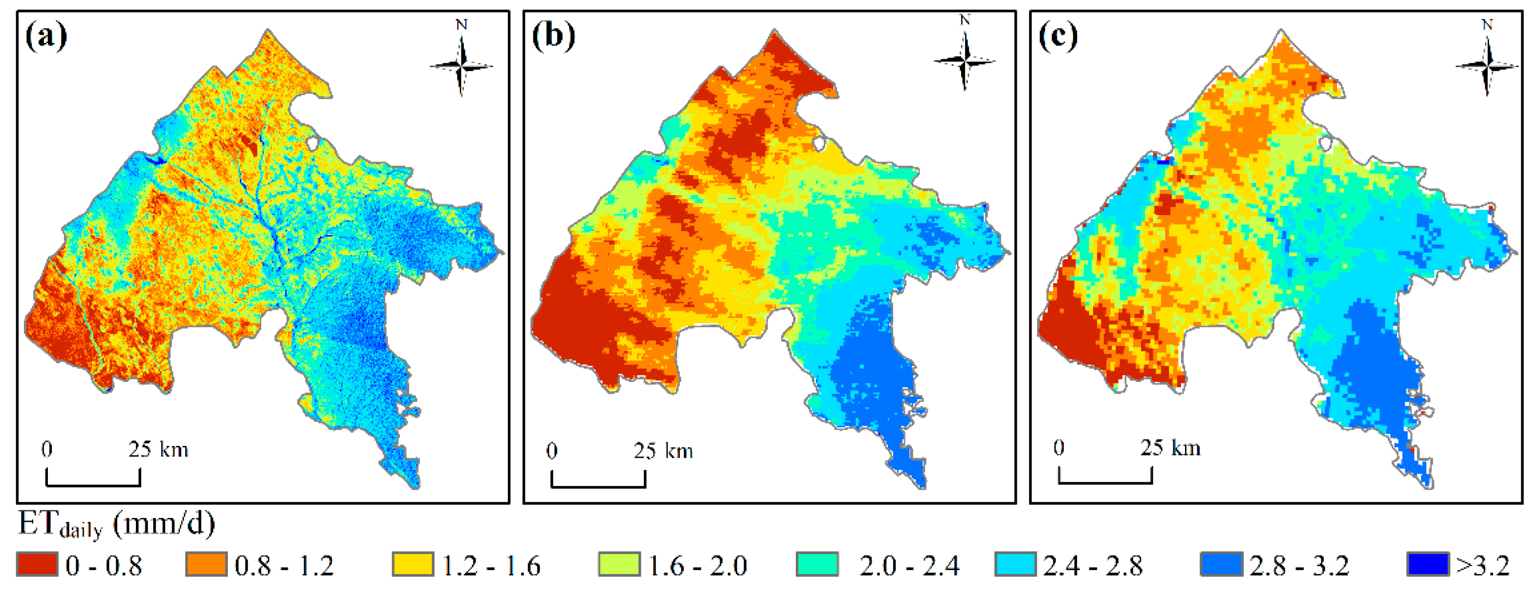
Figure 4 shows the spatial distribution of the simulated ET based on the different sensors. Although the input parameters were derived from the three satellite sensors with different spatial resolutions, the ET simulated using the SEBAL model exhibited similar spatial distribution patterns. Higher heterogeneity and ET values were distributed in the high vegetation density of woods and crops in the southeastern part of the study area. In contrast, lower heterogeneity and ET values were distributed in the grassland and barren land in the northwestern part of the study area (Figure 1b and Figure 4). Landsat TM, which has a spatial resolution of 30 m, can capture the detailed textural features of the land surfaces. The spatial ET patterns based on the Landsat TM data in the mountainous areas with complex terrain in the southeastern part of the study area were well captured compared to the spatial patterns obtained from the MODIS and AVHRR data. For example, the narrow Wuding River valley has a large area of farmland with higher ET values, and can be easily observed in the Landsat TM images, whereas the low spatial resolutions of the ET maps derived from the MODIS and AVHRR data contained mixed pixels and were unable to reflect the detailed heterogeneity of the land surface, making the river valley difficult to observe on the derived ET maps.

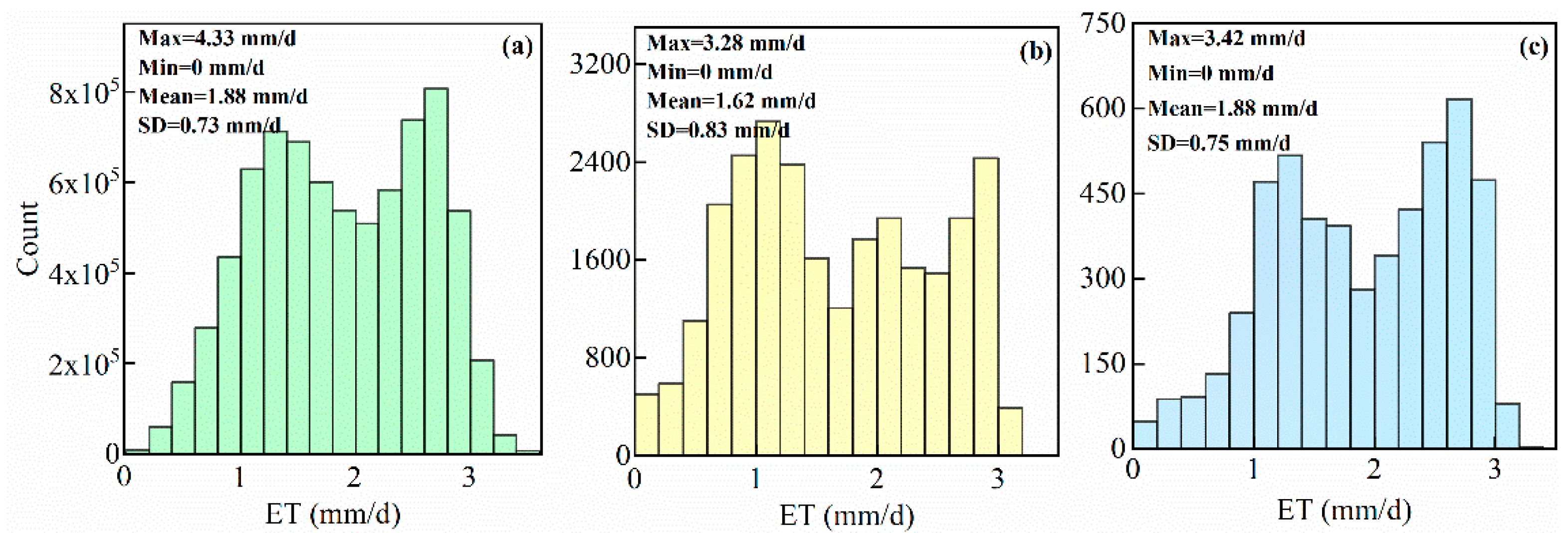
Figure 5 presents the frequency distribution and statistical analysis (mean, maximum, minimum, and standard deviation) of the three datasets. It shows a bimodal distribution among the three datasets. The histogram shapes of ET_Landsat and ET_AVHRR were similar and had two peak frequencies at 1.2–1.4 mm/d and 2.6–2.8 mm/d, respectively. However, the ET_MODIS histogram had peak frequencies at approximately 1.0–1.2 mm/d and 2.8–3.0 mm/d. From the spatial statistical characteristics, the maximum value of ET_Landsat was 4.33 mm/d, followed by ET_AVHRR (3.42 mm/d), and ET_MODIS (3.28 mm/d). The maximum ET values of the three datasets indicated a gradually decreasing trend from finer to coarser spatial resolution datasets.

In summary, the above analyses indicated that the different datasets affected the ET values and statistical characteristics. The coarser spatial resolution data had the larger uncertainty and the MODIS data underestimated the ET value with the largest discrepancies.

3.2. Effects of Aggregation on the Energy Balance Components and ET Estimation

In order to evaluate the effect of input parameter aggregation on the results of the SEBAL model, we used simple averaging schemes to aggregate the input parameters from the original 30 m × 30 m spatial resolution to 1200 m × 1200 m at intervals of 30 m to test the responses of the four energy-balance components to changes in spatial scale, including R_n, G, H, and LE. The spatial means, MRE, and CV were used to quantify the variations of the four fluxes during the aggregation process.

Figure 6 shows the statistical results of the SEBAL input parameter aggregation. The spatial mean and spatial heterogeneity of the NDVI and albedo showed larger changes than other parameters. However, the spatial distribution of the T_s and U were obtained by interpolation, showing limited changes for spatial scale aggregation.

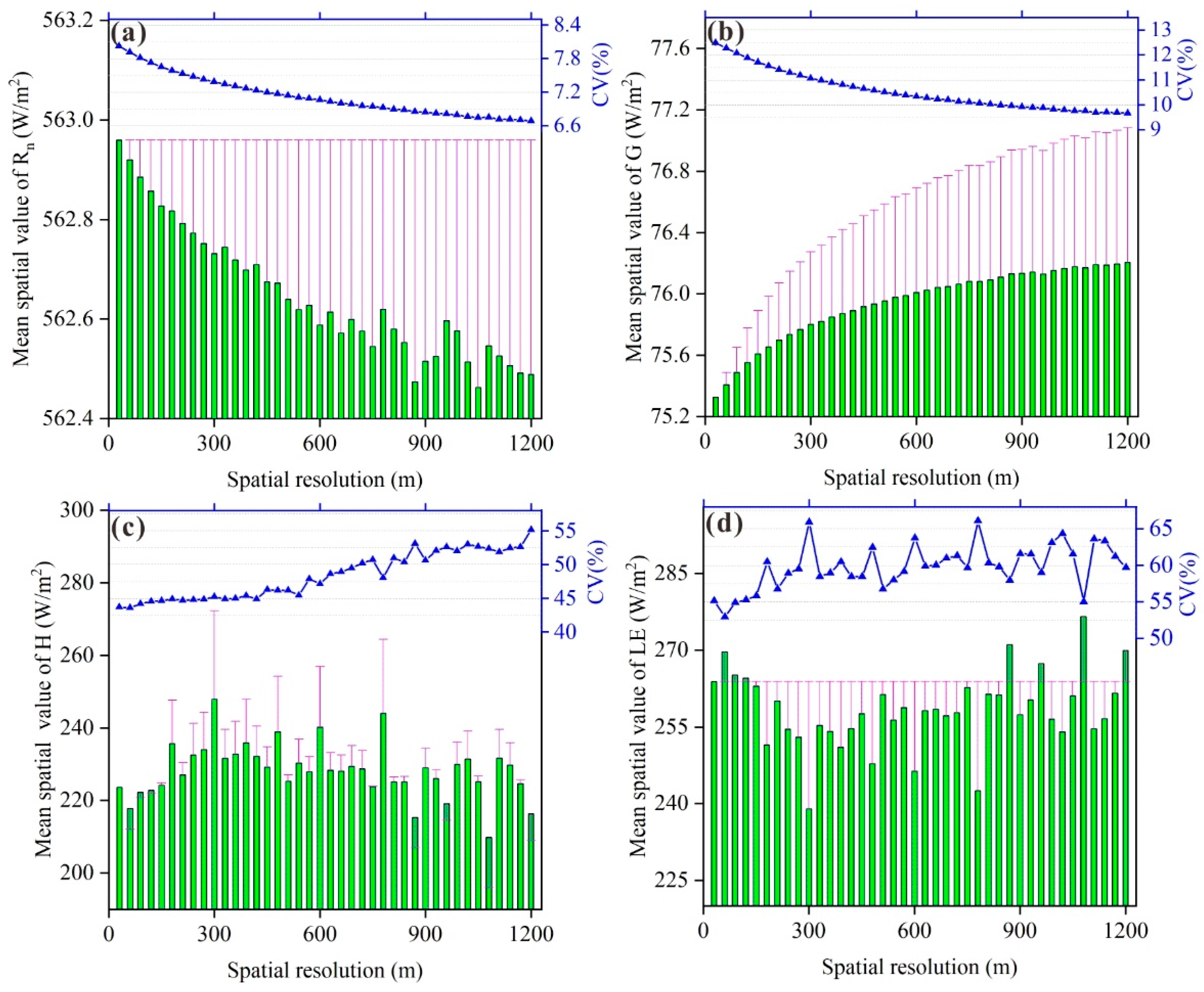
Figure 7 shows the statistical characteristics of the spatial mean and spatial heterogeneity of the fluxes calculated at different aggregation levels. There was a decreasing trend in the spatial mean values of R_n when finer resolution data were aggregated to a coarser resolution, ranging from 562.96 W/m² to 562.46 W/m² and the MRE was −0.06%. In contrast, the spatial mean value of G tended to increase, ranging from 75.33 W/m² to 76.21 W/m². G was slightly overestimated when the finer scale data were aggregated to a coarser scale, and the MRE was 0.82%. All errors exhibited a relatively steady increase. In terms of spatial variability, a relatively small CV was present in the R_n and G (6.68–8.02%, 9.65–12.49%, respectively). The spatial CV of R_n and G showed similar variations: a decreasing tendency when the scale was aggregated, indicating a decrease in spatial heterogeneity. Overall, scale aggregation had limited effects on the R_n and G.

In contrast, the scale aggregation had greater effects and more significant variations on the H and LE than on the R_n and G. The spatial mean values and CV had fluctuating variations. The spatial mean value of the H initially increased, then decreased, ranging from 209.80 W/m² to 247.96 W/m². The MRE of the H was 3.03% and RE reached a maximum of 10.88% at a spatial resolution of 300 m. The spatial mean value of the LE first decreased, and then increased, ranging from 238.97 W/m² to 276.58 W/m², and the MRE was −2.80%. The RE reached a maximum of −9.46% at a spatial resolution of 300 m. The relatively larger CV was present in both the H and LE estimations (43.58–55.14%, 52.94–66.12%, respectively) and had an increasing spatial heterogeneity trend with scale aggregation.

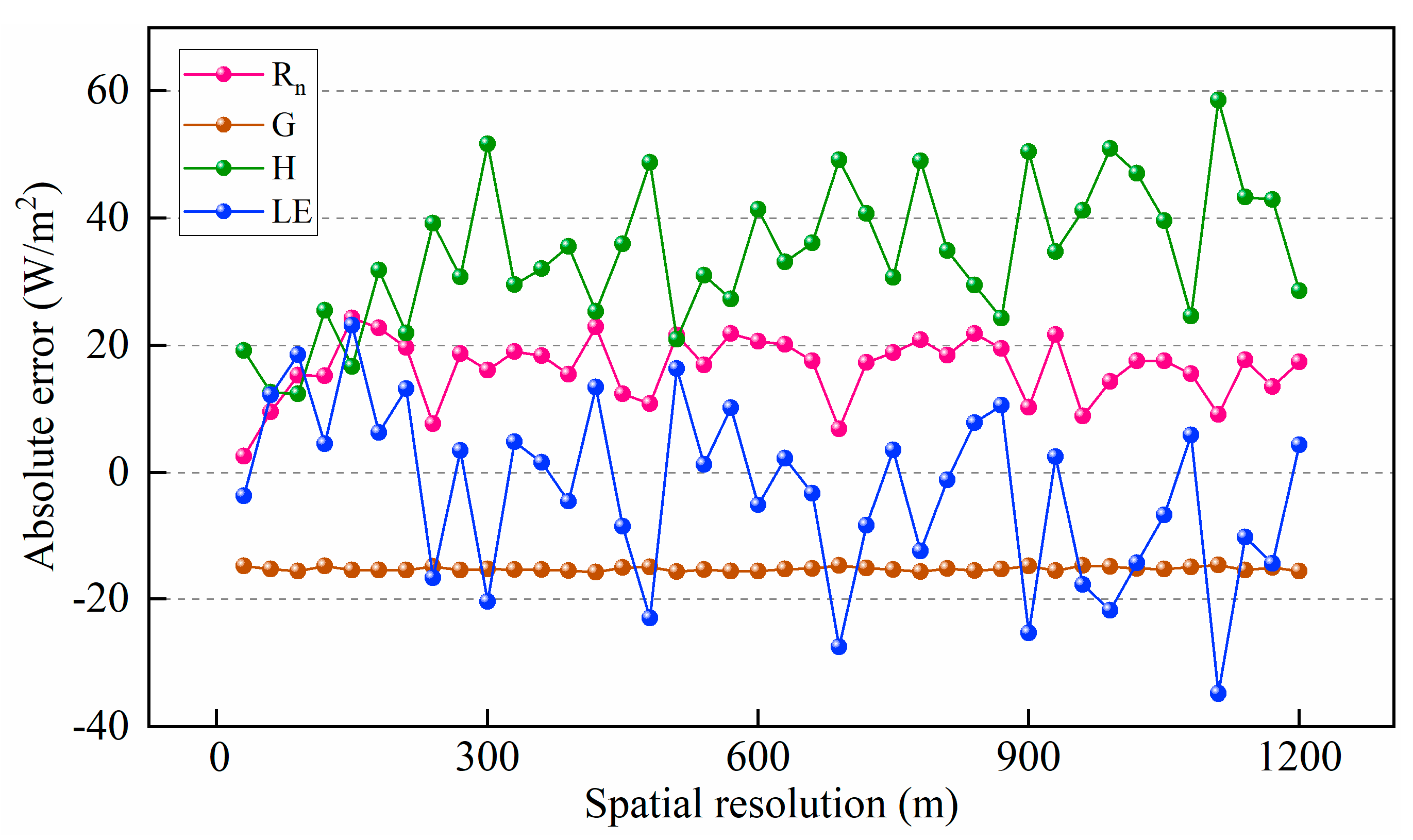
To evaluate the error variation for scale aggregation, we compared the estimated fluxes at different scales with the observed data. We used the Bowen ratio adjustment method reported in Twine et al. [69] to modify the latent and sensible heat fluxes to solve the energy balance closure issue of the eddy covariance flux. Figure 8 shows the AE between the modified flux observation from the YLEOS and the simulated fluxes at different spatial resolutions. The results indicate that the R_n and G values are similar to the original values (at 30 m resolution) and showed relatively little error variation in the scale aggregation (AE values: ~10–20 W/m² and ~−15 W/m², respectively). However, when the pixels were enlarged, the differences between the tower flux data and model output of the H yielded a relative larger error, i.e., AE values increased from 20 W/m² to 60 W/m². The LE error showed a similar tendency to the H, but in the opposite direction, i.e., AE decreased from 0 W/m² to −30 W/m². This implies that the H is the main source of the error during the scale aggregation.

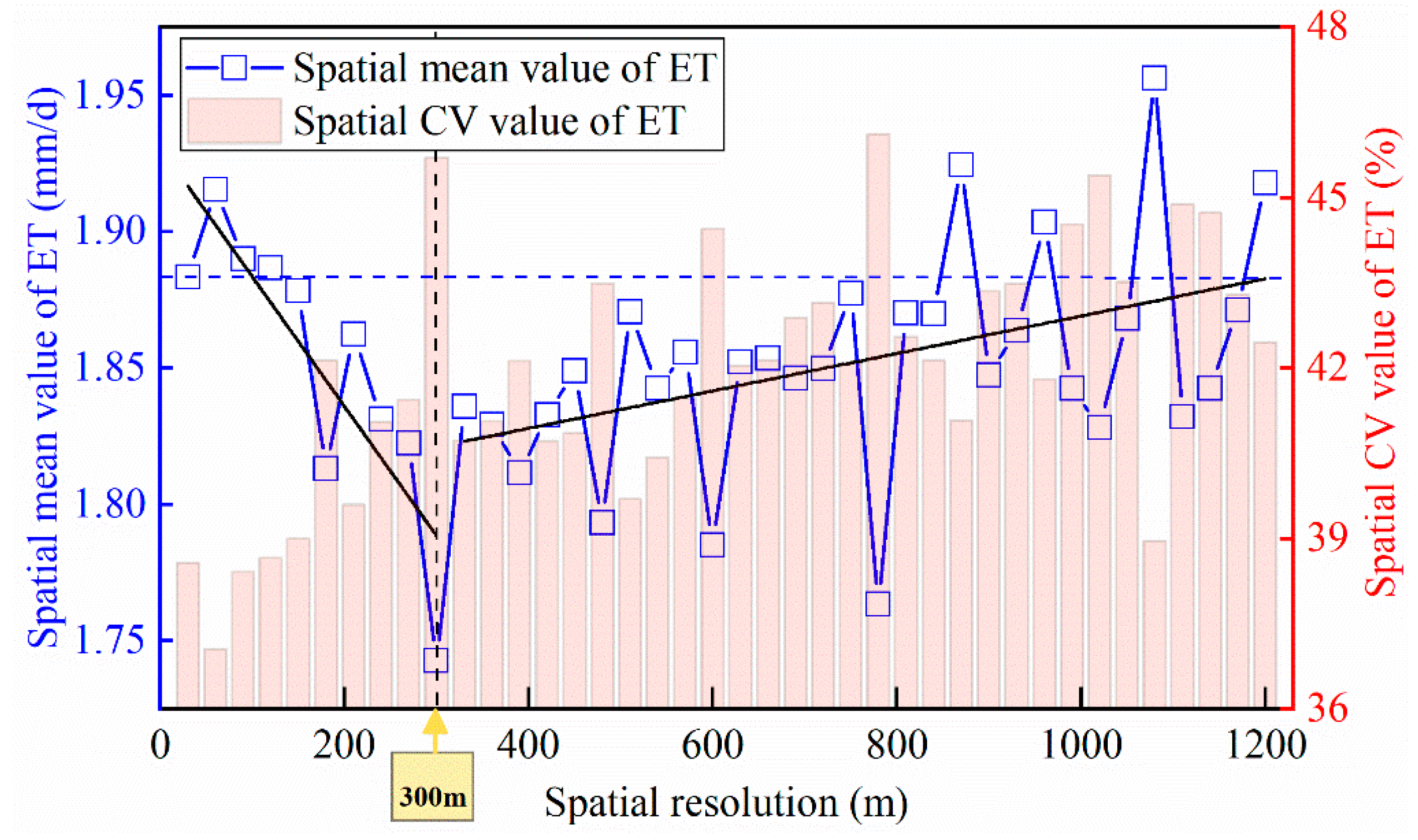
Figure 9 shows the statistics of the daily ET estimations with the scale aggregation. The spatial means of the daily ET initially decreased, then increased with the scale aggregation, ranging from 1.74 mm/d to 1.96 mm/d. A spatial resolution of 300 m was a critical point in the ET simulation scale aggregation. In addition, the spatial heterogeneity increased (CV ranged from 37.05% to 46.12%) with the spatial scale aggregation. We also found that the largest ET values corresponded to smaller spatial heterogeneities. This implies that spatial aggregation affects the SEBAL model simulation processes and performance in a complex way.

3.3. The Effects of Land Use/Cover Pattern on the ET Estimation during the Aggregation Process

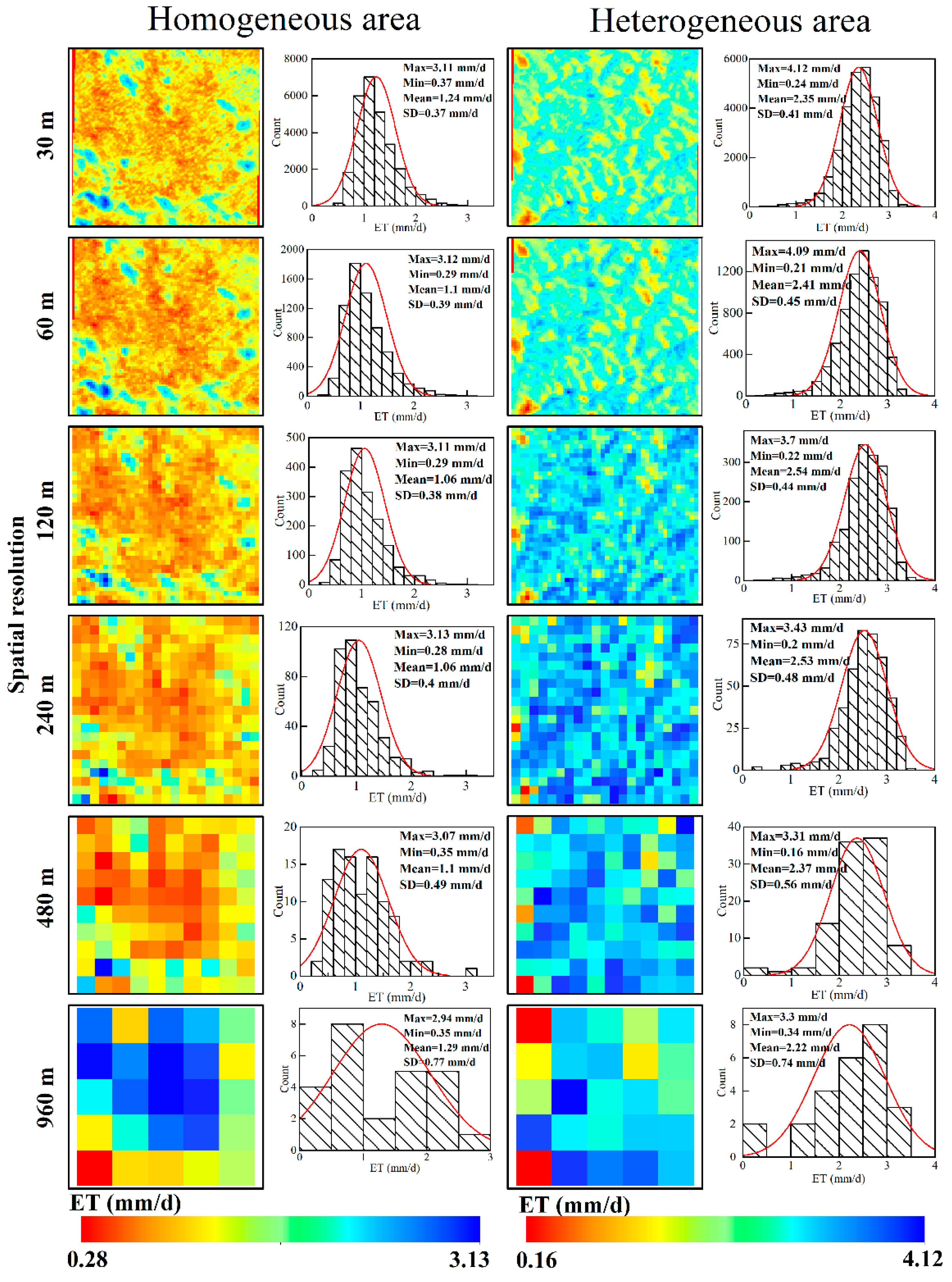
The aggregation effect is mainly caused by non-linear processes in the model mechanisms and surface heterogeneity [17,18] as discussed in Section 3.2. To demonstrate the effect of land use/cover pattern on the ET estimation, two comparison groups (homogeneous and heterogeneous areas) were used to illustrate the changes in the ET estimation during the aggregation process. We selected the following representative nodes of the spatial resolution aggregation results to compare the spatial patterns of the ET estimates: 30 m (original), 60 m, 120 m, 240 m, 480 m, and 960 m (coarse).

Table 5. Statistical results of the energy fluxes in the homogeneous and heterogeneous areas at different spatial resolutions.

Homogeneous Area									Heterogeneous Area
	Rn	AE	G	AE	H	AE	LE	AE	Rn	AE	G	AE	H	AE	LE	AE
30 m	512.75	-	81.64	-	293.64	-	137.47	-	603.16	-	65.88	-	164.35	-	372.93	-
60 m	512.61	−0.14	81.7	0.06	317.5	23.86	113.41	−24.06	603.14	−0.02	65.98	0.10	153.07	−11.28	384.09	11.16
120 m	512.49	−0.26	81.8	0.16	325.48	31.84	105.21	−32.26	603.02	−0.14	66.12	0.24	128.36	−35.99	408.54	35.61
240 m	512.44	−0.31	81.89	0.25	327.42	33.78	103.13	−34.34	602.93	−0.23	66.26	0.38	129.78	−34.57	406.89	33.96
480 m	511.32	−1.43	81.95	0.31	315.98	22.34	113.39	−24.08	603.3	−0.14	66.34	0.46	160.51	−3.84	376.45	3.52
960 m	511.26	−1.49	82.00	0.36	283.22	−10.42	146.04	8.57	603.37	0.21	66.39	0.51	189.37	25.02	347.61	−25.32

Note: R_n represents net radiation flux; G represents soil heat flux; LE represents latent heat flux; H represents sensible heat flux; and AE represents absolute error—all units are W/m².

shows the four energy balance components of the statistical analysis results over the homogeneous and heterogeneous areas at different spatial resolutions. The R_n and G were minimally affected by the different land use/cover pattern with the scale aggregation, and the maximum absolute error was less than 1 W/m². The maximum error of the H in the heterogeneous area was −35.99 W/m² at the spatial resolution of 120 m, while the maximum error of the H in the homogeneous area was −33.78 W/m² at the spatial resolution of 240 m.

Figure 10 shows the spatial distributions and basic statistics of the simulated ET on the different surfaces at different spatial scales. We found that the maximum ET values decreased from fine to coarser resolutions, independent of the land use/cover type. Higher spatial resolutions of 30 m, 60 m, and 120 m preserved the detailed spatial patterns and textural features. For spatial resolutions of 240 m, 480 m, and 960 m, the small surface features disappeared and the spatial structures were obscured, resulting in larger statistical errors in the ET estimation. This indicates that lower spatial resolutions, fewer pixels, and higher spatial variabilities, all contributed to the uncertainty in the ET estimation. Particularly, at a spatial resolution of 960 m, much spatial information was lost, and the spatial patterns, ranges, and magnitudes of ET were degraded.

In the homogeneous area, patches of the grassland with higher ET values were spatially smaller, while the barren land covered a larger area and had lower ET values. After spatial pixel aggregation, the grassland patches lost clear boundaries and produced drastically high and low ET values. The peak of the histogram shifted to a low-value area. The spatial means decreased from 1.24 mm/d at the spatial resolution of 30 m to 1.06 mm/d at the spatial resolution of 240 m. The spatial heterogeneity also increased with the scale aggregation and the standard deviation increased from 0.37 mm/d to 0.77 mm/d. Likewise, in the heterogeneous area, farmland and grassland were staggered after the scale aggregation, the peak of the histogram shifted to the high-value area, the mean and maximum ET values decreased, and the standard deviation increased from 0.41 mm/d at the 30 m spatial resolution to 0.74 mm/d at the spatial resolution of 960 m, which indicates that the pixel aggregation increased both ET estimation errors and spatial heterogeneity.

4. Discussion

4.1. Estimation of the ET from the Three Different Satellite Sensors

Multiple satellites have been launched to obtain Earth observations, with sensors with different spatial, temporal, spectral, and radiation resolutions would usually cause uncertainties in estimating surface fluxes. The ET estimated using multiple sensors (ET_Landsat, ET_MODIS, and ET_AVHRR) with different spatial resolutions were compared in this study. As shown in Section 3.1, both the spatial characterization and frequency distribution of the results demonstrate the similar results between the Landsat TM and AVHRR datasets. However, the MODIS data had the largest uncertainty. The results are similar to those of other studies [14,37,70]. The largest uncertainty in the ET_MODIS could be caused by the following reasons: (1) the original thermal infrared band of MODIS has a spatial resolution of 1 km, and re-sampling may increase its spatial variability; (2) the influence of wavelength range and input parameter calculation methods resulted in the lower ET values; and (3) the difference of about 0.26 mm/d in the spatial mean between the ET_MODIS and ET_Landsat is consistent with the 30 min time gap between the overpass times of the two satellites, the time gap leads to the variation in the EF, causing the difference in the daily ET.

The validation of the RS-based ET at large scales is difficult due to discrepancies in spatial resolution between the ground measurements and remote sensing datasets [30,70]. Generally, input parameters with a higher resolution correspond to the ET estimates with higher accuracy [18,71]. In this study, we observed that finer spatial resolutions did not match the highest ET accuracies. Gaur et al. [47] reported that a high spatial resolution may lead to the underestimation of ET values, and thus, a higher resolution dataset was not necessarily the best choice. This is caused by the mismatch between the flux tower site position and the pixel. The main contributing source area of the YLEOS determined by the footprint model was approximately 1263 m wide and 1682 m long [53], which matches the spatial resolution (1.1 km) of the AVHRR pixels and explains the reason for the higher simulation accuracy of the AVHRR data. Therefore, verifications of the ET simulations with in situ observations must consider the match of the spatial scales.

4.2. Aggregation Effects on the Energy Balance Flux Simulation

Land–atmosphere interaction processes respond non-linearly to changes in scale, and land surface heterogeneities make the scaling process more complicated [4,27,34]. The effect of the spatial resolution on the energy balance components in the SEBAL model was assessed in this study. The results indicate that the R_n and G has the limited changes in scale, while the H and LE yielded relatively larger errors with the spatial scale aggregation. This was also reported by Su et al. [34], Ershadi et al. [30], and Ramírez-Cuesta et al. [27]. The R_n is computed as the algebraic sum of the incoming and outgoing short wave and long wave radiation at the surface, and is closely related to the T_s, T_a, albedo, and NDVI (Equation (2) and Figure 2). Small changes in the T_s and T_a values were observed at an aggregated resolution (Figure 6). The increases in the albedo and NDVI resulted in a small increase in the R_n. The G was calculated with the empirical relation using the R_n, albedo, and NDVI (Equation (3)), which are linearly combined, producing similar small decreasing trends.

Since aggregation tends to average out small surface features, it will introduce more mixed pixels. The difference between the aggregated imagery and the original fine-resolution imagery increases with the aggregation level [18]. This explains why the CV of H and LE increased with the pixel size. As the SEBAL algorithm is non-linear, the changes in the spatial resolution could impact the turbulent heat flux calculations, resulting in a spatial scale discrepancy [34]. A relatively larger error in the aggregation found in the H could be explained by the combined effect of the aerodynamic resistance on heat transfer and the aggregated roughness properties of the surface (z_om) in the SEBAL model (Figure 2 and Equations (4)–(7)). However, the U and T_s underwent relatively small changes, suggesting that the aerodynamic resistance could be the reason for the changes in the H when the scale was aggregated. Differences in the H at different pixel resolutions highlight the important role of z_om parameterization in the flux estimation, which is directly related to the changes in NDVI.

In addition, the acquisition of aerodynamic resistance requires local calibration by the user to select cold and hot pixels in specific image scenes using multiple iterative steps, which exhibits a highly nonlinear relationship. A sensitivity analysis of the SEBAL model confirmed that the changes in the H are very sensitive to the selection of hot and cold pixels [21,72]. Compared with the low-resolution data, the high-resolution satellite data have fewer mixed pixels and the extremely hot and cold pixels are more readily identified. When the scale is aggregated, (1) it changes the locations of the hot and cold pixels in the T_s images at the various spatial resolutions; (2) it introduces more land surface information, causing the value of the hot and cold pixels to decrease as the scale is enlarged, which could result in large deviations in the slope and intercept of the linear relationship between dT and T_s (Equations (4)–(6) and Figure 11), resulting in a larger error in the H. The non-linear changes in the cold and hot pixel values also explain why the multiple high and low values were present in the ET trend during the scale aggregation.

In general, the variation in the surface temperature for the selected extreme pixels (hot pixels and cold pixels) at the different spatial resolution are a major reason for the ET uncertainty in the ET simulation.

4.3. Influence of the Land Use/Cover Pattern on the ET Estimates during the Aggregation Process

ET estimates using remote sensing data are largely affected by plant structure, canopy characteristics, and the proportion of bare soil present in a pixel [47]. A scale change could alter the composition of land cover in a pixel, which creates differences in the ET variance. This study indicates that the land use/cover pattern has obvious effects on the ET simulation using the different RS products. In addition, we also determined that a different pattern of land use/cover exhibited different aggregation results. As Figure 1d and Figure 10 show in the homogeneous areas, the aggregation of the small grassland patches with higher ET values to large barren land patches with lower ET values decreased the maximum value of the ET, which in turn decreases the spatial average values of the ET. The aggregation process in the heterogeneous areas is dominated by the mixing of the high ET farmland and low ET grassland patches, increasing the maximum value of the ET during the aggregation, and in turn raising the overall spatial means of the ET. We also found that the land cover has a much greater impact on the H and LE than on the R_n and G (Table 5). Unexpectedly, we found that regardless of the complexity of the land use/cover pattern, the entire land surface affected the ET aggregation results. This is because the aggregation increases the number of mixed pixels over the homogeneous and heterogeneous areas and affects the selection of the hot and cold pixels, resulting in the changes to the ET simulation. This illustrates that the effect of the model mechanisms is greater than the impact of the land use/cover pattern in the SEBAL model simulation.

4.4. Limitations and Outlook

In this study, we examined the effect of spatial aggregation on the ET simulations. However, the transit times of satellites, spectral resolutions and parameter estimation methods may also affect the analysis of the multi-sensor estimated ET values. Future studies should choose datasets with the same or closer transit times to evaluate the scale aggregation effects. In addition, there is only one in situ flux site available in the study area of the present study. If feasible, in situ data from more flux sites need to be used in the verification of simulation results in future studies.

5. Conclusions

In this study, we investigated the spatial resolution influences on the ET estimation using the SEBAL model. The main conclusions of this study are as follows:

• The spatial distribution patterns of the ET estimates using Landsat TM, MODIS, and AVHRR datasets were similar, with MODIS having the largest uncertainties. The validation of the simulated ET must consider matching spatial scales of the satellite datasets.
• With scale aggregation, the spatial average values of the R_n decreased slightly, while the G increased, and the spatial variabilities of both R_n and G all decreased. The spatial mean values of the H and LE were relatively larger, but the relative error was less than 20%. This was due to the changes in the selection of the locations of the hot and cold pixels in the model mechanisms as well as the NDVI and surface albedo input parameters in the SEBAL model.
• Surface heterogeneity affected the spatial scale aggregation results, and differences in the land use/cover pattern led to the different aggregation results. However, the scale errors caused by the SEBAL model mechanisms were larger than that contributed by the land use/cover pattern during the scale aggregation.

References

1. Wood, E.F.; Sivapalan, M.; Beven, K.; Band, L. Effects of spatial variability and scale with implications to hydrologic modeling. J. Hydrol. 1988, 102, 29–47. [Google Scholar] [CrossRef]
2. Goodrich, D.C.; Lane, L.J.; Shillito, R.M.; Miller, S.N.; Syed, K.H.; Woolhiser, D.A. Linearity of basin response as a function of scale in a semiarid watershed. Water Resour. Res. 1997, 33, 2951–2965. [Google Scholar] [CrossRef]
3. Brunsell, N.A.; Gillies, R.R. Scale issues in land–atmosphere interactions: Implications for remote sensing of the surface energy balance. Agric. Forest Meteorol. 2003, 117, 203–221. [Google Scholar] [CrossRef]
4. Sridhar, V.; Elliott, R.L.; Chen, F. Scaling effects on modeled surface energy-balance components using the NOAH-OSU land surface model. J. Hydrol. 2003, 280, 105–123. [Google Scholar] [CrossRef]
5. Brunsell, N.A.; Anderson, M.C. Characterizing the multi–scale spatial structure of remotely sensed evapotranspiration with information theory. Biogeosciences 2011, 8, 2269–2280. [Google Scholar] [CrossRef] [Green Version]
6. Schulze, R. Transcending scales of space and time in impact studies of climate and climate change on agrohydrological responses. Agric. Ecosyst. Environ. 2000, 82, 185–212. [Google Scholar] [CrossRef]
7. Wallender, W.W.; Grismer, M.E. Irrigation hydrology: Crossing scales. J. Irrig. Drain. Eng. 2002, 128, 203–211. [Google Scholar] [CrossRef]
8. Simic, A.; Chen, J.M.; Liu, J.; Csillag, F. Spatial scaling of net primary productivity using subpixel information. Remote Sens. Environ. 2004, 93, 246–258. [Google Scholar] [CrossRef]
9. Yu, Z.; Lu, Q.; Zhu, J.; Yang, C.; Ju, Q.; Yang, T.; Chen, X.; Sudicky, E.A. Spatial and temporal scale effect in simulating hydrologic processes in a watershed. J. Hydrol. Eng. 2014, 19, 99–107. [Google Scholar] [CrossRef]
10. Oki, T.; Kanae, S. Global hydrological cycles and world water resources. Science 2006, 313, 1068–1072. [Google Scholar] [CrossRef] [PubMed] [Green Version]
11. Batra, N.; Islam, S.; Venturini, V.; Bisht, G.; Jiang, L. Estimation and comparison of evapotranspiration from MODIS and AVHRR sensors for clear sky days over the southern great plains. Remote Sens. Environ. 2006, 103, 1–5. [Google Scholar] [CrossRef]
12. Fisher, J.B.; Melton, F.; Middleton, E.; Hain, C.; Anderson, M.; Allen, R.; Kilic, A. The future of evapotranspiration: Global requirements for ecosystem functioning, carbon and climate feedbacks, agricultural management, and water resources. Water Resour. Res. 2017, 53, 2618–2626. [Google Scholar] [CrossRef]
13. Xu, X.F.; Li, X.L.; Wang, X.J.; He, C.S.; Tian, W.; Tian, J.; Yang, L.X. Estimating daily evapotranspiration in the agricultural-pastoral ecotone in Northwest China: A comparative analysis of the Complementary Relationship, WRF-CLM4.0, and WRF-Noah methods. Sci. Total Environ. 2020, 138635. [Google Scholar] [CrossRef] [PubMed]
14. Mauser, W.; Schädlich, S. Modelling the spatial distribution of evapotranspiration on different scales using remote sensing data. J. Hydrol. 1998, 212–213, 250–267. [Google Scholar] [CrossRef]
15. Zhang, K.; Kimball, J.S.; Nemani, R.R.; Running, S.W. A continuous satellite-derived global record of land surface evapotranspiration from 1983 to 2006. Water Resour. Res. 2010, 46, W09522. [Google Scholar] [CrossRef] [Green Version]
16. Yang, Y.T.; Long, D.; Shang, S.H. Remote estimation of terrestrial evapotranspiration without using meteorological data. Geophys. Res. Lett. 2013, 40, 3026–3030. [Google Scholar] [CrossRef]
17. Hong, S.H.; Hendrickx, J.M.H.; Borchers, B. Up-scaling of SEBAL derived evapotranspiration maps from Landsat (30 m) to MODIS (250 m) scale. J. Hydrol. 2009, 370, 122–138. [Google Scholar] [CrossRef]
18. Sharma, V.; Kilic, A.; Irmak, S. Impact of scale/resolution on evapotranspiration from Landsat and MODIS images. Water Resour. Res. 2016, 52, 1800–1819. [Google Scholar] [CrossRef] [Green Version]
19. Peng, Z.Q.; Xin, X.; Jiao, J.J.; Zhou, T.; Liu, Q. Remote sensing algorithm for surface evapotranspiration considering landscape and statistical effects on mixed pixels. Hydrol. Earth Syst. Sci. 2016, 20, 4409–4438. [Google Scholar] [CrossRef] [Green Version]
20. Gebremichael, M.; Wang, J.; Sammis, T.W. Dependence of remote sensing evapotranspiration algorithm on spatial resolution. Atmos. Res. 2010, 96, 489–495. [Google Scholar] [CrossRef]
21. Tang, R.; Li, Z.; Chen, K.; Jia, Y.; Li, C.; Sun, X. Spatial-scale effect on the SEBAL model for evapotranspiration estimation using remote sensing data. Agric. For. Meteorol. 2013, 174–175, 28–42. [Google Scholar] [CrossRef]
22. Wang, S.; Li, X.; Ge, Y.; Jin, R.; Ma, M.; Liu, Q.; Wen, J.; Liu, S. Validation of regional-scale remote sensing products in China: From Site to Network. Remote Sens. 2016, 8, 980. [Google Scholar] [CrossRef] [Green Version]
23. Liu, S.; Xu, Z.; Song, L.; Zhao, Q.; Ge, Y.; Xu, T.; Ma, Y.; Zhu, Z.; Jia, Z.; Zhang, F. Upscaling evapotranspiration measurements from multi-site to the satellite pixel scale over heterogeneous land surfaces. Agric. For. Meteorol. 2016, 230–231, 97–113. [Google Scholar] [CrossRef]
24. Liang, S. Quantitative Remote Sensing of Land Surfaces; John Wiley and Sons, Inc.: Hoboken, NJ, USA, 2004. [Google Scholar]
25. Hong, S.H.; Hendrickx, J.M.H.; Borchers, B. Effect of scaling transfer between evapotranspiration maps derived from Landsat 7 and MODIS images. In targets and backgrounds XI: Characterization and representation. Int. Soc. Opt. Photonic 2005, 5811, 147–158. [Google Scholar]
26. Sun, Z.; Gebremichael, M.; Ardo, J.; Nickless, A.; Caquet, B.; Merboldh, L.; Kutschi, W. Estimation of daily evapotranspiration over Africa using MODIS/Terra and SEVIRI/MSG data. Atmos. Res. 2012, 112, 35–44. [Google Scholar] [CrossRef]
27. Ramírez-Cuesta, J.M.; Allen, R.G.; Zarcotejada, P.J.; Kilic, A.; Santos, C.; Lorite, I.J. Impact of the spatial resolution on the energy balance components on an open-canopy olive orchard. Int. J. Appl. Earth Obs. Geoinf. 2019, 88–102. [Google Scholar] [CrossRef]
28. Gao, X.; Sun, M.; Luan, Q.; Zhao, X.; Wang, J.; He, G.; Zhao, Y. The spatial and temporal evolution of the actual evapotranspiration based on the remote sensing method in the Loess Plateau. Sci. Total Environ. 2020, 708, 135111. [Google Scholar] [CrossRef]
29. Weng, Q. Remote sensing of impervious surfaces in the urban area: Requirements, methods: And trends. Remote Sens. Environ. 2012, 117, 34–49. [Google Scholar] [CrossRef]
30. Ershadi, A.; Mccabe, M.F.; Evans, J.P.; Walker, J.P. Effects of spatial aggregation on the multi-scale estimation of evapotranspiration. Remote Sens. Environ. 2013, 131, 51–62. [Google Scholar] [CrossRef]
31. Wang, Y.Q.; Xiong, Y.J.; Qiu, G.Y.; Zhang, Q. Is scale really a challenge in evapotranspiration estimation? A multi-scale study in the Heihe oasis using thermal remote sensing and the three-temperature model. Agric. Forest Meteorol. 2016, 230–231, 128–141. [Google Scholar] [CrossRef]
32. Henderson-Sellers, A.; Wilson, M.F.; Thomas, G. The effect of spatial resolution on archives of land cover type. Clim. Change. 1985, 7, 391–402. [Google Scholar] [CrossRef]
33. Moran, M.S.; Humes, K.S.; Pinter, P.J. The scaling characteristics of remotely-sensed variables for sparsely-vegetated heterogeneous landscapes. J. Hydrol. 1997, 190, 337–362. [Google Scholar] [CrossRef]
34. Su, Z.; Pelgrum, H.; Menenti, M. Aggregation effects of surface heterogeneity in land surface processes. Hydrol. Earth Syst. Sci. 1999, 3, 549–563. [Google Scholar] [CrossRef] [Green Version]
35. Liang, S. Numerical experiments on the spatial scaling of land surface albedo and leaf area index. Remote Sens. Rev. 2000, 19, 225–242. [Google Scholar] [CrossRef]
36. Long, D.; Singh, V.P.; Li, Z.L. How sensitive is SEBAL to changes in input variables, domain size and satellite sensor? J. Geophys. Res. Atmos. 2011, 116, D21107. [Google Scholar] [CrossRef]
37. McCabe, M.F.; Wood, E.F. Scale influences on the remote estimation of evapotranspiration using multiple satellite sensors. Remote Sens. Environ. 2006, 105, 271–285. [Google Scholar] [CrossRef]
38. Semmens, K.A.; Anderson, M.C.; Kustas, W.P.; Gao, F.; Alfieri, J.G.; Mckee, L.; Prueger, J.H.; Hain, C.R.; Cammalleri, C.; Yang, Y.; et al. Monitoring daily evapotranspiration over two California vineyards using Landsat 8 in a multi-sensor data fusion approach. Remote Sens. Environ. 2016, 185, 155–170. [Google Scholar] [CrossRef] [Green Version]
39. Vinukollu, R.K.; Wood, E.F.; Ferguson, C.R.; Fisher, J.B. Global estimates of evapotranspiration for climate studies using multi-sensor remote sensing data: Evaluation of three process-based approaches. Remote Sens. Environ. 2011, 115, 801–823. [Google Scholar] [CrossRef]
40. Elhaddad, A.; Garcia, L.A.; Chavez, J.L. Using a surface energy balance model to calculate spatially distributed actual evapotranspiration. J. Irrig. Drain. Eng. 2011, 137, 17–26. [Google Scholar] [CrossRef]
41. Su, Z. The Surface Energy Balance System (SEBS) for estimation of turbulent heat fluxes. Hydrol. Earth Syst. Sci. 2002, 6, 85–100. [Google Scholar] [CrossRef]
42. Bastiaanssen, W.G.; Menenti, M.; Feddes, R.A.; Holtslag, A.A. A remote sensing surface energy balance algorithm for land (SEBAL); 1 formulation. J. Hydrol. 1998, 212, 198–212. [Google Scholar] [CrossRef]
43. Allen, R.G.; Tasumi, M.; Trezza, R. Satellite-based energy balance for mapping evapotranspiration with internalized calibration (MERTIC)-model. J. Irrig. Drain. Eng. 2007, 133, 380–394. [Google Scholar] [CrossRef]
44. Norman, J.M.; Kustas, W.P.; Humes, K.S. Source approach for estimating soil and vegetation energy fluxes in observations of directional radiometric surface temperature. Agric. For. Meteorol. 1995, 77, 263–293. [Google Scholar] [CrossRef]
45. Kustas, W.P.; Li, F.; Jackson, T.J.; Prueger, J.H.; Macpherson, J.I.; Wolde, M. Effects of remote sensing pixel resolution on modeled energy flux variability of croplands in Iowa. Remote Sens. Environ. 2004, 92, 535–547. [Google Scholar] [CrossRef]
46. Roerink, G.; Su, Z.; Menenti, M. S-SEBI: A simple remote sensing algorithm to estimate the surface energy balance. Phys. Chem. Earth B Hydrol. Ocean. Atmos. 2000, 25, 147–157. [Google Scholar] [CrossRef]
47. Gaur, N.; Mohanty, B.P.; Kefauver, S.C. Effect of observation scale on remote sensing based estimates of evapotranspiration in a semi-arid row cropped orchard environment. Prec. Agric. 2017, 18, 762–778. [Google Scholar] [CrossRef]
48. Bastiaanssen, W.G.; Noordman, E.J.; Pelgrum, H.; Davids, G.; Thoreson, B.; Allen, R.G. SEBAL model with remotely sensed data to improve water-resources management under actual field conditions. J. Irrig. Drain. Eng. 2005, 131, 85–93. [Google Scholar] [CrossRef]
49. Mo, X.G.; Liu, S.X.; Chen, D.; Lin, Z.H.; Guo, R.P.; Wang, K. Grid-size effects on estimation of evapotranspiration and gross primary production over a large Loess Plateau basin, China. Hydrol. Sci. J. 2009, 54, 160–173. [Google Scholar] [CrossRef]
50. Xue, Y.Y.; Zhang, B.Q.; He, C.S.; Shao, R. Detecting vegetation variations and main drivers over the agropastoral ecotone of northern china through the ensemble empirical mode decomposition method. Remote Sens. 2019, 11, 1860. [Google Scholar] [CrossRef] [Green Version]
51. Wang, X.J.; Zhang, B.Q.; Xu, X.F.; Tian, J.; He, C.S. Regional water-energy cycle response to land use/cover change in the agro-pastoral ecotone, Northwest China. J. Hydrol. 2020, 580, 124246. [Google Scholar] [CrossRef]
52. Han, Z.B.; Zhang, B.Q.; Yang, L.X.; He, C.S. Assessment of the impact of future climate change on maize yield and water use efficiency in agro-pastoral ecotone of Northwestern China. J. Agro. Crop. Sci. 2021, 207, 1–15. [Google Scholar] [CrossRef]
53. Gong, T.T.; Lei, H.M.; Yang, D.W.; Jiao, Y.; Yang, H.B. Monitoring the variations of evapotranspiration due to land use/cover change in a semiarid shrubland. Hydrol. Earth Syst. Sci. 2017, 21, 863–877. [Google Scholar] [CrossRef] [Green Version]
54. Matthew, M.W.; Adler-Golden, S.M.; Berk, A.; Felde, G.; Anderson, G.P.; Gorodestzky, D.; Paswaters, S.; Shippert, M. Atmosphere correction of spectral imagery. Evaluation of the FLAASH algorithm with AVIRIS data. Presented at the SPIE Proceeding, Algorithms and Technologies for Multispectral, Hyperspectral, and Ultraspectral Imagery IX, Washington, DC, USA, 16–18 October 2002. [Google Scholar]
55. Nemani, R.R.; Running, S.W. Estimation of regional surface resistance to evapotranspiration from NDVI and Thermal-IR AVHRR data. J. Appl. Meteorol. 1989, 28, 276–284. [Google Scholar] [CrossRef]
56. Bastiaanssen, W.G.M. SEBAL-based sensible and latent heat fluxes in the irrigated Gediz Basin, Turkey. J. Hydrol. 2000, 229, 87–100. [Google Scholar] [CrossRef]
57. Allen, R.G.; Irmak, A.; Trezza, R.; Hendrickx, J.M.; Bastiaanssen, W.G.; Kjaersgaard, J. Satellite-based ET estimation in agriculture using SEBAL and METRIC. Hydrol. Proc. 2011, 25, 4011–4027. [Google Scholar] [CrossRef]
58. Allen, R.G.; Pereira, L.S.; Raes, D.; Smith, M. Crop Evapotranspiration: Guidelines for Computing Crop Requirements; FAO Irrigation and Drainage Paper 56; Food and Agricultural Organization of the U.N.: Rome, Italy, 1998. [Google Scholar]
59. Clothier, B.E.; Clawson, K.L.; Pinter, J.P.J.; Moran, M.S.; Reginato, R.J.; Jackson, R.D. Estimation of soil heat flux from net radiation during growth of alfalfa. Agric. For. Meteorol. 1986, 37, 319–329. [Google Scholar] [CrossRef]
60. Brutsaert, W. Evaporation into the Atmosphere; D. Reidel Pub. Co.: Dordrecht, The Netherlands, 1982. [Google Scholar] [CrossRef]
61. Su, Z.; Jacobs, C. ENVISAT: Actual Evaporation. BCRS Report 2001: USP-2 Report 2001; Publication of the National Remote Sensing Board (BCRS): Delft, The Netherlans, 2001. [Google Scholar]
62. Shuttleworth, W.J.; Gurney, R.J.; Hsu, A.Y.; Ormsby, J.P. Fife: The variation in energy partition at surface flux sites. IAHS Publ. 1989, 186, 67–74. [Google Scholar]
63. Crago, R.D. Conservation and variability of the evaporative fraction during the daytime. J. Hydrol. 1996, 180, 173–194. [Google Scholar] [CrossRef]
64. Bian, L.; Butler, R. Comparing effects of aggregation methods on statistical and spatial properties of simulated spatial data. Photogram. Eng. Remote Sens. 1999, 65, 73–84. [Google Scholar] [CrossRef]
65. Famiglietti, J.S.; Wood, E.F. Multiscale modelling of spatially variable water and energy balance processes. Water Resour. Res. 1994, 30, 3061–3078. [Google Scholar] [CrossRef] [Green Version]
66. Willmott, C.J. Some comments on the evaluation of model performance. Bull. Am. Meteorol. Soc. 1982, 63, 1309–1369. [Google Scholar] [CrossRef] [Green Version]
67. Yu, D.; Li, X.; Cao, Q.; Hao, R.; Qiao, J. Impacts of climate variability and landscape pattern change on evapotranspiration in a grassland landscape mosaic. Hydrol. Proc. 2020, 34, 1035–1051. [Google Scholar] [CrossRef]
68. McGarigal, K.; Cushman, S.A.; Neel, M.C.; Ene, E. FRAGSTATS: Spatial Pattern Analysis Program for Categorical Maps. Computer Software Program Produced by the Authors at the University of Massachusetts, Amherst. 2002. Available online: http://www.umass.edu/landeco/research/fragstats/fragstats.html (accessed on 23 March 2020).
69. Twine, T.E.; Kustas, W.P.; Norman, J.M.; Cook, D.R.; Houser, P.R.; Meyers, T.P.; Prueger, J.H.; Starks, P.J.; Wesely, M.L. Correcting eddy-covariance flux underestimates over a grassland. Agric. For. Meteorol. 2000, 103, 279–300. [Google Scholar] [CrossRef] [Green Version]
70. Jia, Z.; Liu, S.; Xu, Z.; Chen, Y.; Zhu, M. Validation of remotely sensed evapotranspiration over the Hai River Basin, China. J. Geophys. Res. 2012, 117, D13113. [Google Scholar] [CrossRef]
71. Tian, H.; Wen, J.; Wang, C.; Liu, R.; Lu, D. Effect of pixel scale on evapotranspiration estimation by remote sensing over oasis areas in north-western China. Environ. Earth Sci. 2012, 67, 2301–2313. [Google Scholar] [CrossRef]
72. Wang, J.; Sammis, T.W.; Gutschick, V.P.; Gebremichael, M.; Miller, D.R. Sensitivity analysis of the surface energy balance algorithm for land (SEBAL). Trans. ASABE 2009, 52, 801–811. [Google Scholar] [CrossRef]
Figure 1. Map of the study area: (a) location of the study area (the Yuyang District) in the agro-pastoral ecotone, Northwestern China and locations of meteorological stations; (b) land use/cover map of the study area and location of the homogeneous and heterogeneous area and flux tower site; (c) DEM and water network; (d) characteristics of the homogeneous and heterogeneous areas. YLEOS refers to the Yulin Ecohydrological Observation Station, Tsinghua University.
Remotesensing 13 01524 g001
Figure 2. Flowchart for the Surface Energy Balance Algorithm for Land (SEBAL) model algorithms. NDVI is normalized difference vegetation index, ET is evapotranspiration, and LE is latent heat flux.
Remotesensing 13 01524 g002
Figure 3. Flowchart of the ET simulation and aggregation processes. Landsat TM is Landsat Thematic Mapper, MODIS is Moderate Resolution Imaging Spectroradiometer, and AVHRR is Advanced Very High-Resolution Radiometer.
Remotesensing 13 01524 g003
Figure 4. Spatial distribution of ET estimates by (a) Landsat TM, (b) MODIS, and (c) AVHRR over the Yuyang District on 7 August 2011. Transit time for Landsat TM is approximately 11:07 (local time: GMT + 8), for MODIS is approximately 10:30 (local time), and for AVHRR is approximately 10:02 (local time).
Remotesensing 13 01524 g004
Figure 5. Frequency distribution and statistics of the ET estimates from (a) Landsat TM, (b) MODIS and (c) AVHRR.
Remotesensing 13 01524 g005
Figure 6. Change of the spatial mean and spatial heterogeneity of the SEBAL input parameters at different spatial resolutions.
Remotesensing 13 01524 g006
Figure 7. Statistical characteristics of the spatial means and spatial heterogeneity of the fluxes calculated at different aggregation levels: (a) net radiation flux; (b) soil heat flux; (c) sensible heat flux; and (d) latent heat flux (the green bars represent the spatial mean of different resolutions, the pink lines represent errors compared to the initial resolution (30 m), and the blue lines represent the coefficient of variation).
Remotesensing 13 01524 g007
Figure 8. Absolute error variation between the eddy covariance observed fluxes and the SEBAL simulated fluxes at different spatial resolutions.
Remotesensing 13 01524 g008
Figure 9. Spatial mean values and coefficients of variation of the simulated ET at different spatial resolutions (the blue dotted line represents the value of the estimated ET at spatial resolution at 30 m, the black dotted represent the critical point at the spatial resolution of 300 m).
Remotesensing 13 01524 g009
Figure 10. Spatial and frequency distribution of the simulated ET over homogeneous and heterogeneous areas at different spatial resolutions.
Remotesensing 13 01524 g010
Figure 11. Locations and values of the (a) hot pixels and (b) cold pixels at different spatial resolutions.
Remotesensing 13 01524 g011