Abstract
In the scenario of high dynamics and low C/N0, the discriminator output of a GNSS tracking loop is noisy and nonlinear. The traditional method uses a fixed-gain loop filter for error estimation, which is prone to lose lock and causes inaccurate navigation and positioning. This paper proposes a cascaded adaptive vector tracking method based on the KF+EKF architecture through the GNSS Software defined receiver in the signal tracking module and the navigation solution module. The linear relationships between the pseudo-range error and the code phase error, the pseudo-range rate error and the carrier frequency error are obtained as the measurement, and the navigation filter estimation is performed. The signal C/N0 ratio and innovation sequence are used to adjust the measurement noise covariance matrix and the process noise covariance matrix, respectively. Then, the estimated error value is used to correct the navigation parameters and fed back to the local code/carrier NCO. The field vehicle test results show that, in the case of sufficient satellite signals, the positioning error of the proposed method has a slight advantage compared with the traditional method. When there is signal occlusion or interference, the traditional method cannot achieve accurate positioning. However, the proposed method can maintain the same accuracy for the positioning results.
1. Introduction
With the upgrading of satellite navigation systems, such as the GPS in the United States, BeiDou in China, Galileo in Europe, and Quasi-Zenith in Japan, the Global Navigation Satellite System (GNSS) receiver technology is also stimulating new vitality. Its main function is to use the local replica signal to synchronize with the input signal, and decode the ephemeris to obtain the position, velocity, and time (PVT) information. Software receivers are favored by the majority of scholars because of more potential advantages of algorithm scalability, flexibility, and high module repeatability [1].
Reliable GNSS data can provide auxiliary information for aerial photography, geodetic surveying, and other remote sensing fields to improve the measurement accuracy of the target area. As a special scenario of remote sensing, Intelligent Transportation has attracted more attention in the Internet of Things (IoT). When vehicles or unmanned autonomous vehicles are driving in the urban environment and encounter tall buildings or dense trees, the proposed method can still maintain high navigation and positioning information. According to the multi-sensor data provided by the vehicle, they bring a reliable source of information for road monitoring of the entire city. The traffic flow can be adjusted to the best condition to ensure that vehicles can travel freely on the road. Managers can make roads and vehicles more scientific and rigorous for intelligent management and intelligent decision-making.
In the scalar tracking loop, the discriminator output is directly fed back to the Numerically Controlled Oscillator (NCO), which works well in the case of high carrier-to-noise ratio and low dynamics. However, the fixed bandwidth and gain make it easier for the loop to lose lock at a lower Carrier-to-Noise ratio (C/N0). In an ideal situation, the phase error measurement of strong satellite signals should be given more weight than weak signals. Because the different channels of the traditional tracking loop of the GNSS receiver work independently, there is no information sharing between the channels, and it is impossible to excavate all the information of the satellite constellation and the user’s location. According to different filter schemes, the methods adopted mainly include the Phase Lock Loop (PLL)/Delay Lock Loop (DLL), or Frequency Lock Loop (FLL) nonlinear discriminator output as the measurement of the Kalman Filter (KF) [2,3]. They are directly used as baseband I phase and Q phase correlators output inside the tracking loop as measurement of the Extended Kalman Filter (EKF) [4,5,6] and so on. Among them, the nonlinear discriminator output of I and Q signals is used to estimate the signal parameter error, and the matrix design is simple. However, it will cause the measurement noise covariance matrix to lose the Gaussian white noise characteristics. According to the KF theory, the optimal estimation is based on an accurate noise statistical model, otherwise the filtering result will be inaccurate or divergent. Therefore, an adaptive strategy is needed to adjust measurement noise covariance R and process noise covariance matrix Q to improve the robustness and accuracy of the filter. The parameter setting criteria and the influencing factors of the tracking loop are described in detail in [7,8]. According to the selection of different measurement residuals and the establishment of the state matrix, many researchers have also studied the implementation of the KF in different forms to evaluate the performance of different loop tracking methods [9,10,11,12]. By comparing the noise bandwidth, open and closed loop transfer functions, in addition to the use of time-varying gains, these KF methods are mathematically equivalent to traditional methods, and provide a reference for how to adjust the Kalman parameters according to the expected performance.
However, in many harsh scenarios, such as high dynamics, low C/N0 ratio, intermittent signal interruption, multipath interference, non-line-of-sight reception, etc., in order to improve the usability of GNSS receivers in modern navigation applications, the vector tracking-based architecture has aroused widespread attention and discussion in the challenging environment of GNSS. Vector tracking makes full use of the internal relationship between the tracking channels to convert the discriminator output into a pseudo-range error and a pseudo-range rate error. When the navigation solution and satellite ephemeris are known, the code phase error and frequency error of the next epoch are predicted to update the NCO [13]. Many scholars have elaborated on the characteristics of vector tracking algorithms. Lashley [14,15] compares the performance of three adaptive estimation methods in the vector tracking process. Under high dynamic conditions, they all show the same level of error. The performance of the algorithm depends on the specific implementation and debugging, as well as the amount of calculation. As discussed in [16,17], a scalar-vector FLL is proposed in scenarios, such as lack of signal interruption and high dynamics. Under the equivalent noise bandwidth, the performances of the FLL of scalar, least square method, and EKF are analyzed. The KF depends on the appropriate system noise covariance matrix. When the signal is interrupted for a long time, a frequency error lock may occur. Vector tracking can provide more accurate frequency and code phase estimation, but it needs navigation solution information. As presented in [18,19,20,21,22], different forms of robust Vector Phase Lock Loop (VPLL) methods are proposed for the carrier phase joint tracking when GNSS signals suffer from ionospheric scintillation, or for the fast-maneuvering situation, the relationship between filter gain and noise covariance is analyzed. Yang [23] proposed a joint vector carrier tracking scheme to achieve high sensitivity and flexible parameter selection. It mainly includes a separate loop for each channel to track the specific dynamics of the satellite and the total channel based on the EKF to track the common dynamics of different channels. The structure of EKF-based software receivers is analyzed in [24], including special modules for tracking loop initialization and maintenance, and NCO update rules. As far as the final positioning accuracy is concerned, the advantages and disadvantages of the EKF and traditional FLL/PLL+DLL are compared. As described in [25], a simple classification of existing vector tracking methods is carried out. Under noisy or high dynamic environments, the performances of vector receiver and traditional receiver are compared. The advantages of vector tracking are: (1) the best user state estimation is obtained by combining different measurement noises; (2) the weak signal is assisted by a strong signal; (3) after the satellite signal is lost, it is reacquired.
Combining the main points of the above paper, the improvement of the accuracy and robustness of GNSS signals in challenging environments, such as dense forests, urban canyons, satellite occlusion, and signal attenuation are topics worthy of discussion. We present an adaptive cascaded vector tracking loop frame design. In the signal tracking loop, the KF is used to accurately estimate the code phase error, carrier phase error, and carrier frequency error, which are converted into pseudo-range and pseudo-range rate errors, and applied to the navigation solution module based on the EKF. Because the output of the nonlinear discriminator is non-Gaussian, it results in inaccurate and even divergent filtering effects. The process noise variance matrix and the measurement noise variance matrix are adjusted by the innovation orthogonality and C/N0 estimation method. The advantages of the proposed method in positioning accuracy, tracking loop stability, and C/N0 estimation are presented through the vehicle test.
This paper is organized as follows: Section 2 explains the design of cascaded adaptive vector tracking loop. It mainly includes the basic principles of the signal tracking loop method based on the KF and the extended Kalman navigation filter. The method of adaptively adjusting the noise covariance matrix is also mentioned. Section 3 mainly covers experiments using a field vehicle and analyzes the navigation and positioning solution results, demonstrating the validity of the proposed method. Discussion and conclusions are drawn in Section 4.
2. Design of Cascaded Adaptive Vector Tracking Loop
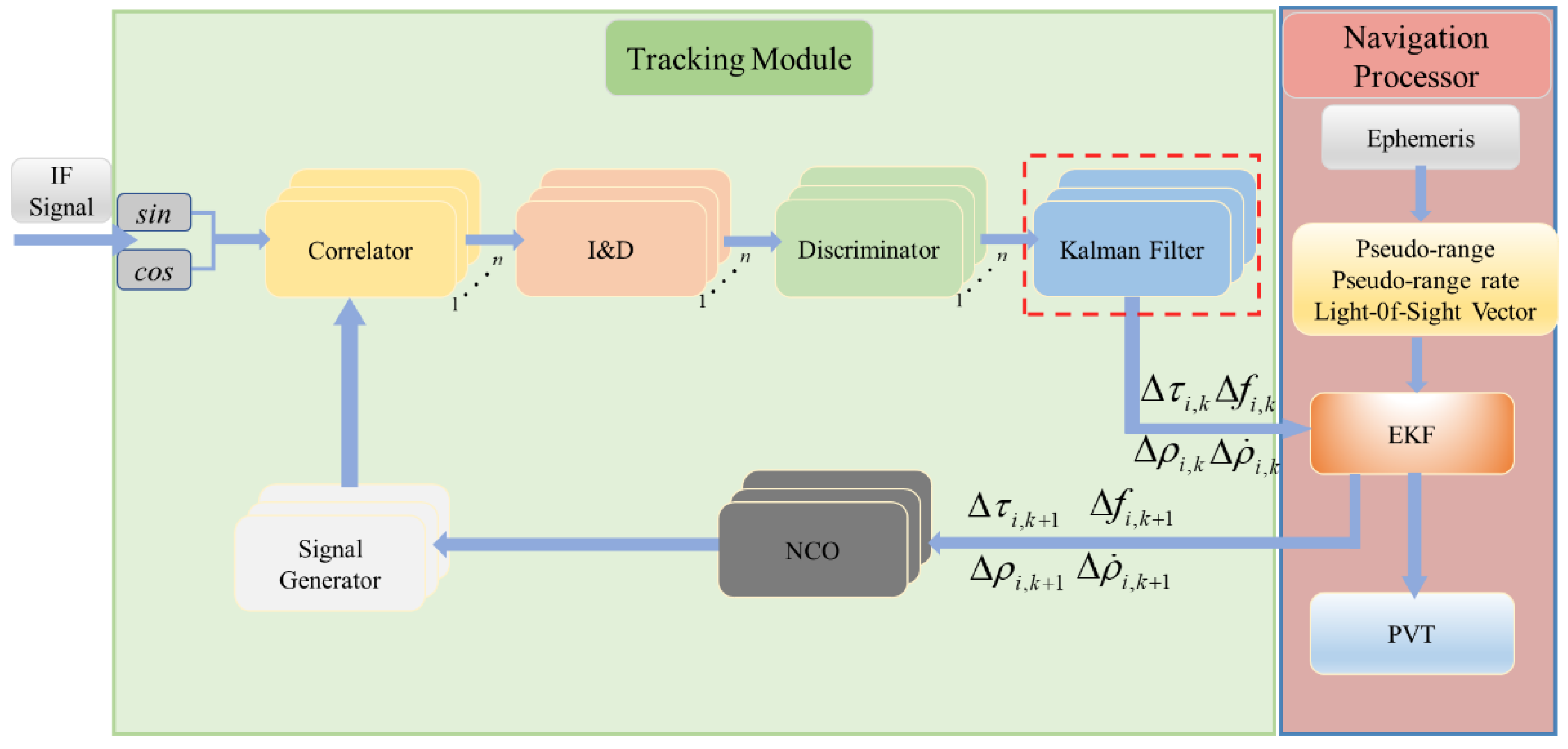
The vector tracking loop can share information between channels. The measurement noise is distributed in the form of weights to estimate accurately the loop phase error and improve the dynamic performance and accuracy of the GNSS receiver. In order to achieve GNSS signal acquisition, tracking and positioning solution, the vector tracking loop structure is mainly composed of a code/carrier discriminator, a KF preprocessor, and an EKF navigation solution. The collected intermediate frequency (IF) signals are processed by local signal correlation for coherent integration. The discriminator output is used as the input of the KF. The output information is the code phase error and the carrier phase error. Through a linear transformation, it is converted into a pseudo-range error and a pseudo-range rate error, which are used as the measurement information of the navigation filter processor. The receiver’s PVT and other navigation information are obtained through filter estimation, and the local code/carrier NCO is updated with the calculated pseudo-range and pseudo-range rate to generate a local replica signal. The block diagram is shown in Figure 1.
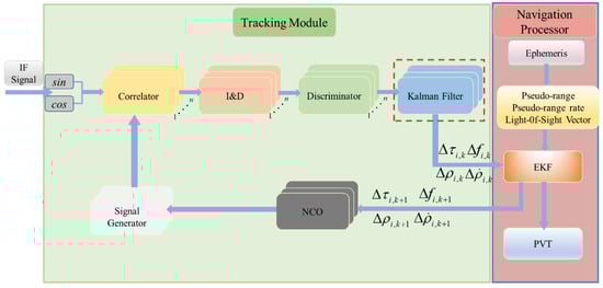
Figure 1.
Design block diagram of adaptive cascaded vector tracking loop.
2.1. Signal Tracking Loop Based on KF
Won [10,11] has proved that the KF method can provide a C/N0 gain of 2–3dB in terms of carrier phase and Doppler tracking. Therefore, in the signal tracking process, the filter equation is established with the code phase error (chips), carrier phase error (rad), and carrier frequency error (Hz), carrier frequency rate error (Hz/s) as the state variables. After discretization, it can be expressed as [22]:
where the coefficient β= is used to convert the units of cycles to units of chips. represent code and carrier frequency. represents the process noise vector. represents time interval...represents the coherent integration time. represents the channel number.
The output of the discriminator is the average value of the carrier phase error and the code phase error (the output is obtained through time integration, called the “average effect”) [1]:
where represents the measurement noise vector.
The code phase error and carrier error are calculated by using the early minus later phase discriminator and the two-quadrant arctangent phase discriminator, respectively:
where are the coherent integral output of the prompt, early, and later forward and quadrature directions of the correlator, respectively.
When the C/N0 ratio is low, the discriminator output is noisy. The adaptive strategy can be used to improve the tracking accuracy of the carrier phase in high dynamic scenarios. Measurement noise depends on the discriminator output and the coherent integration time.
where the diagonal element is proportional to the noise variance of the code phase error and the carrier phase error [5].
where are the error variance values, T is the coherent integration time, and d0 is the code correlator interval.
The C/N0 ratio estimation method adopts the Variance Sum Method (VSM) for each coherent integration output result I, Q (coherent integration time is 20ms) [6]. The main calculation steps are:
The mean and variance of are:
Then the average carrier power can be defined as:
where N is the number of samples of the time series S, and A is the signal amplitude output by the front end.
For the noise part of the I and Q branches, the covariance of the noise integral term is:
The estimated value of the C/N0 is:
2.2. Extended Kalman Navigation Filter Design
This section adopts the receiver position error , receiver velocity error , receiver clock drift, and clock drift rate as the state variables of the EKF navigation processor to establish the state and measurement equations.
where is the discretized state transition matrix, is the state noise matrix, and the statistical characteristics can be expressed as:
where are the variances of the receiver position error, the clock drift, and the clock drift rate, respectively.
The discretized measurement equation can be expressed as:
where represent the pseudo-range error and pseudo-range rate error, m represents the number of satellites, represent the line-of-sight distance vector between the i-th satellite and the receiver, and is the measurement noise. Under the premise of satisfying Gaussian white noise:
According to the linear relationship between code phase error and pseudo-range error , carrier frequency error , and pseudo-range rate error , the establishment of measurement information can be derived:
where are the wavelengths of the C/A chip and the carrier, is the speed of light: 299,792,458 m/s.
The main parameters that affect the performance of the EKF include the process noise matrix Q and the measurement noise covariance matrix R, which are related to the system dynamics and the pre-filter output noise, respectively. When there is unpredictable external interference, the system model may not reflect the true state of motion, the Q and R matrices are directly related to the system model. When the model parameters change, the system parameters need to be adjusted in time to improve the robustness of the filter.
The innovation sequence refers to the difference between the a priori estimate and the latest measurement, which can be used to estimate the measurement noise and system process noise in real time, reduce the model estimation deviation, and obtain an accurate filtering estimate. It is defined as [11]:
The theoretical covariance matrix of the innovation sequence is:
Therefore, the covariance of the innovation sequence in a fixed interval can be obtained through a sliding window to correct the estimate in real time, and then the recursive formula can be used to reduce the amount of calculation:
where , is the forgetting factor, and 0.95 is often taken.
Then,
In addition, the relationship between the innovation sequence and state variables can be derived according to the filter equation:
Then the update equation is:
Then, the basic equation of the EKF navigation in discrete form is:
After the navigation filtering estimation, the position, velocity, and time information are corrected, and then the error state quantity is cleared.
where represent receiver position, velocity, clock drift, and clock drift rate, respectively.
According to the ephemeris and receiver status, the carrier and code frequency for feedback correction of the NCO is predicted.
where is the relative speed between the satellite and the receiver, is intermediate frequency, and is the receiver clock drift rate (m/s).
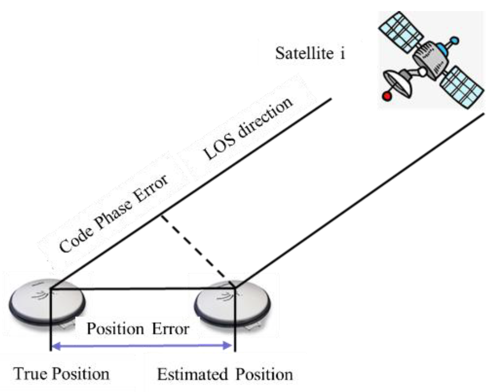
According to the corresponding relationship in Figure 2, the correction value of the code phase change can be derived:
where represents the satellite movement distance in the update period, and then the C/A code phase estimation value can be solved:
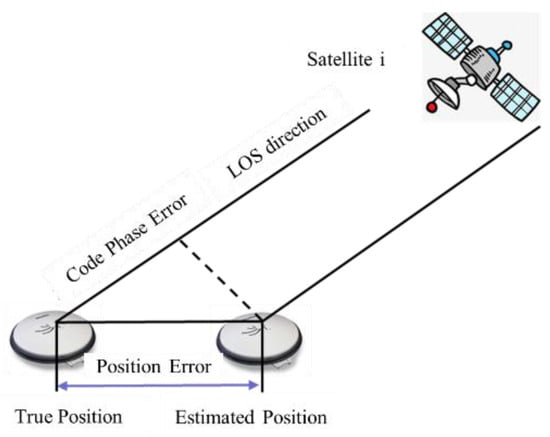
Figure 2.
The relationship between position error and code phase error.
Using the above-mentioned navigation filter output to correct the code phase, code frequency, and carrier frequency in the tracking loop, the receiver vector loop calculation can be completed. Before the vector tracking loop, it is necessary to process the IF signal through the traditional loop, decode the ephemeris, and initialize the PVT information.
3. Experiment and Analysis
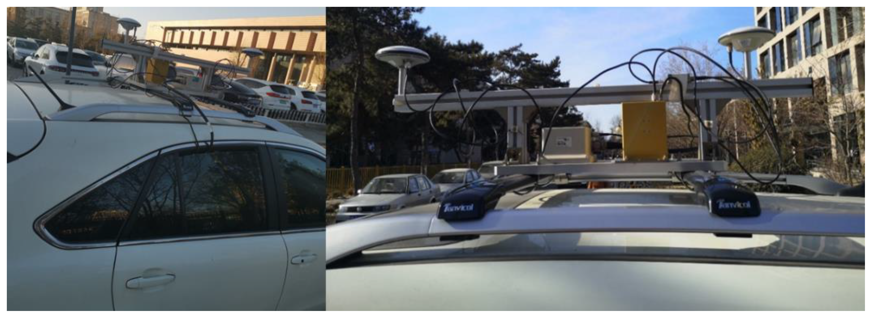
This section will verify the effectiveness and feasibility of the proposed method through three experimental test scenarios. The test equipment is shown in Figure 3. The NovAtel SPAN-CPT high-precision navigation system is used as the measurement benchmark, and the positioning results of the traditional tracking method and the proposed method are compared.

Figure 3.
Experimental environments and setup.
3.1. Static Test Results
First, the antenna was mounted on the roof of an automobile. The vehicle is stationary for 40 s in an open-sky environment, IF data are collected.
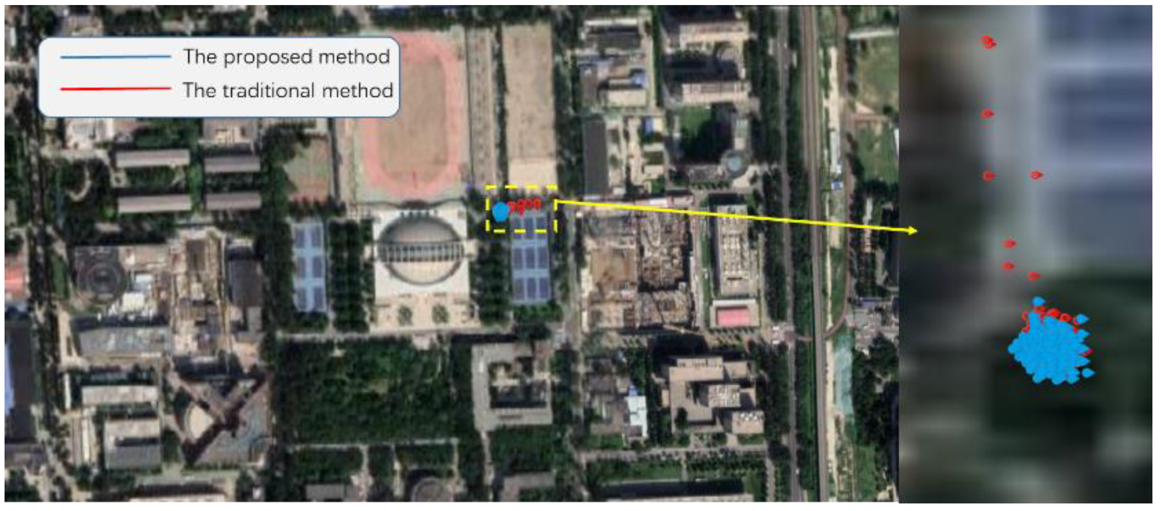
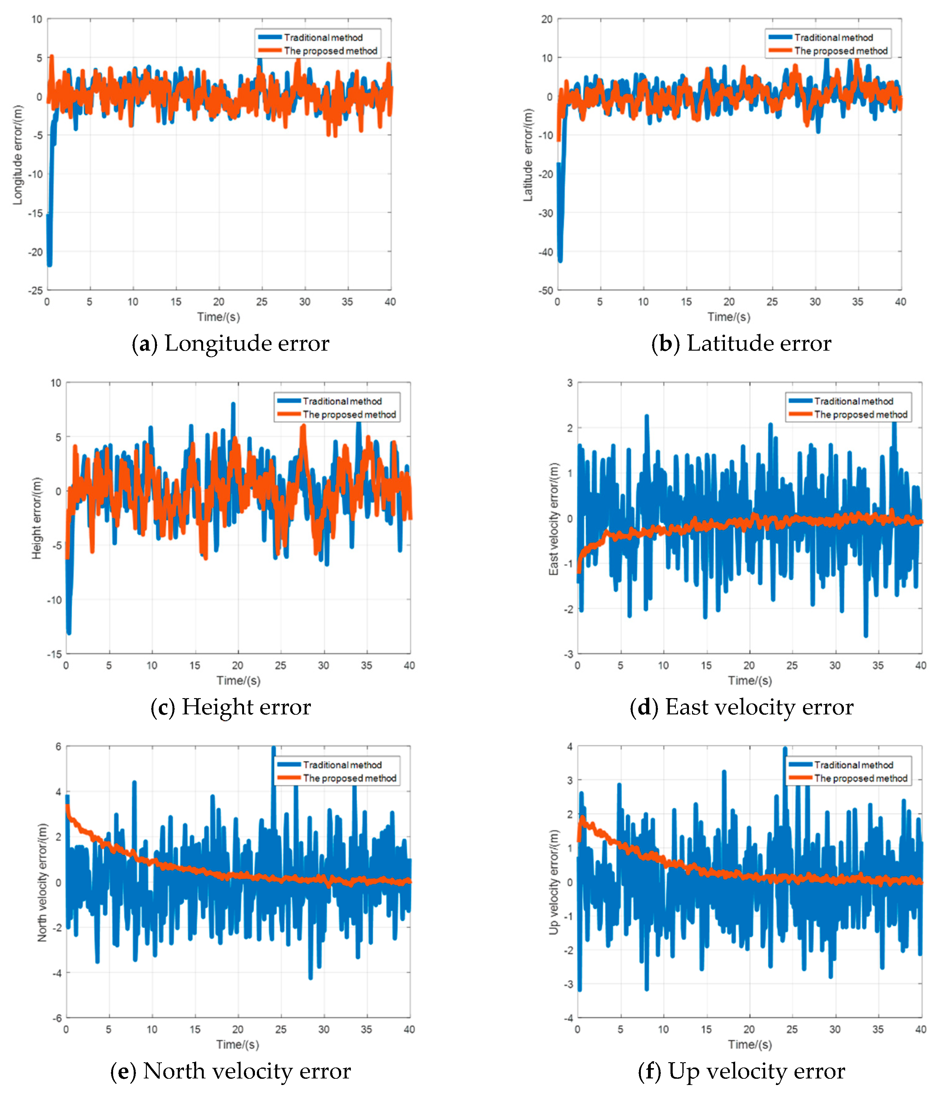
Figure 4 shows the static positioning results in the Google map. Figure 5a–c and Table 1 present the position error and the Root Mean Square Error (RMSE). The proposed method exhibits an RMSE of 1.63 m and 2.85 m in the longitude and latitude directions, respectively. It has a slight advantage compared with 2.50 m and 5.08 m of the traditional method. In the height direction, the error fluctuation ranges of the two methods are basically similar, 2.31 m and 2.67 m, respectively.

Figure 4.
The positioning results in the static test in a Google map.
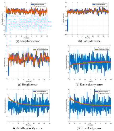
Figure 5.
Comparison results of position error and velocity error in the static test.

Table 1.
Root Mean Square of position error under vehicle stationary condition.
The velocity error results are shown in Figure 5d–f and Table 2. In the east, north, and up direction, the proposed method presents an RMSE of 0.20 m/s, 0.73 m/s, and 0.47 m/s, respectively, compared with 0.87 m/s, 1.56 m/s, and 1.16 m/s of the traditional method. It is obviously superior in terms of stability, and has a more accurate error estimation accuracy.
Table 2.
Root Mean Square of velocity error under vehicle stationary condition.
3.2. Kinematic Test
Figure 6 shows the positioning results of the proposed method, traditional method, and NovAtel reference trajectory through a Google map in urban roads.
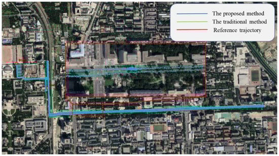
Figure 6.
Kinematic test positioning results in an open-sky area.
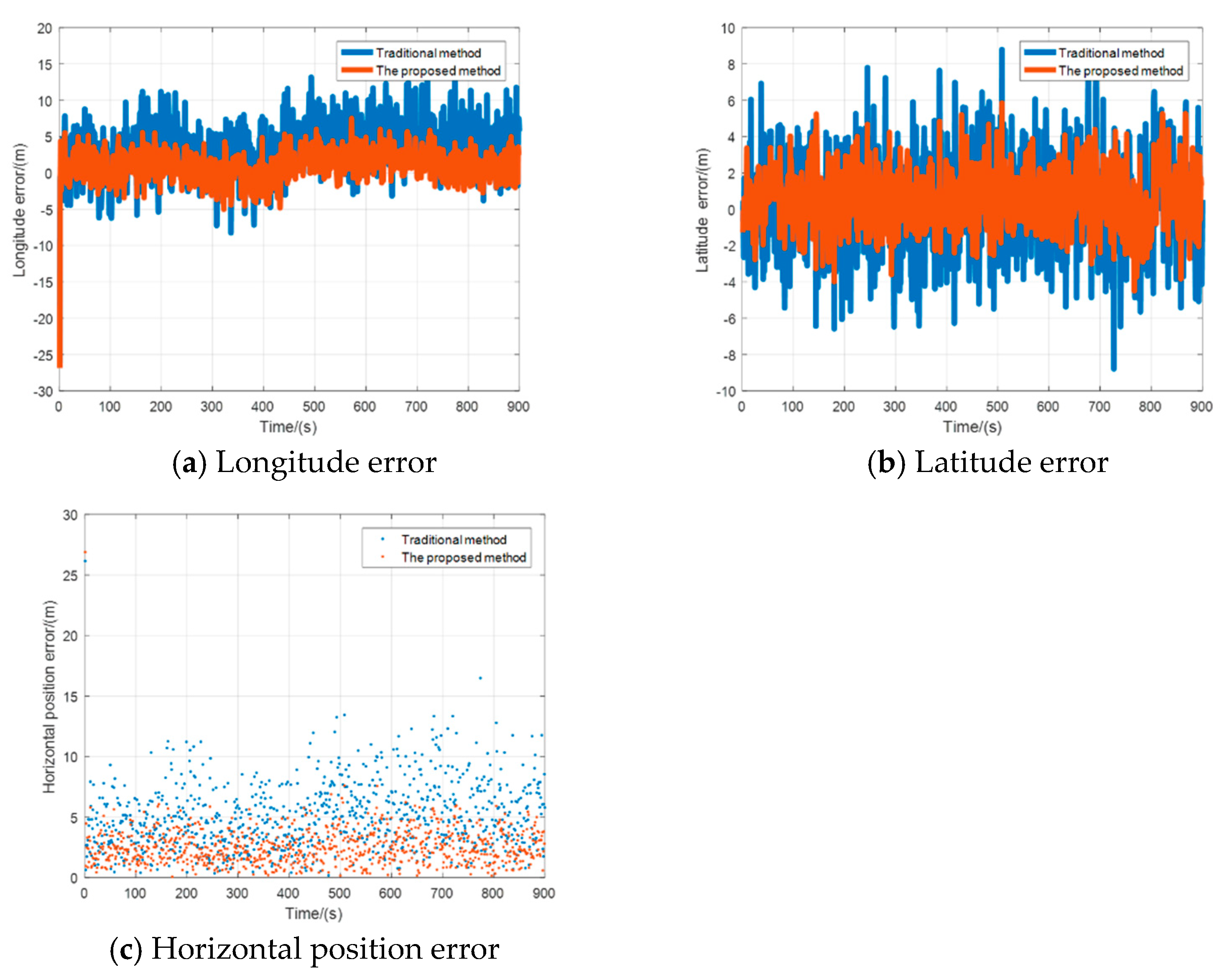
From Figure 7a–c and Table 3, it can be seen that when the number of satellites is normal, the positioning result of the proposed method has a slight advantage over the traditional method, and it shows better positioning stability and accuracy.
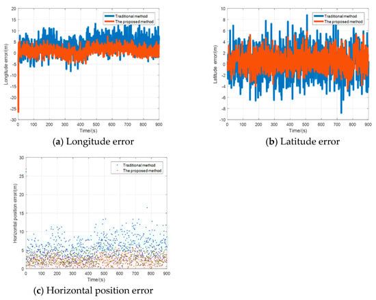
Figure 7.
Comparison result of position error in the kinematic test.
Table 3.
Mean and RMSE of position error under vehicle stationary condition.
3.3. Kinematic Test under Signal Blocking or Interference Occasions
Considering extreme scenarios, when the satellite signal is weak or less than or equal to four satellites, this section performs an interrupt processing on GNSS IF signals and presents the positioning results of different methods under satellite interference conditions. The parameter settings are shown in Table 4.
Table 4.
Signal interruption time and satellite Pseudo Random Noise(PRN) code setting.
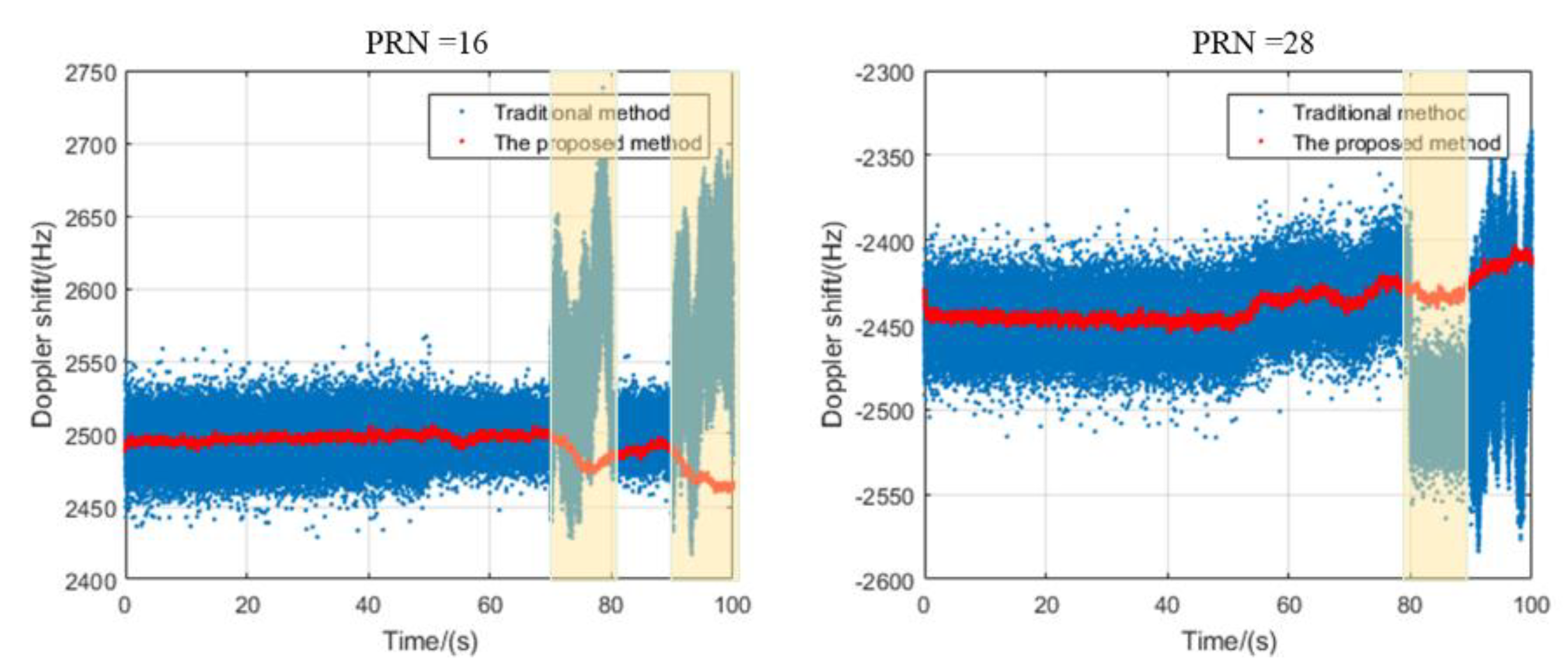
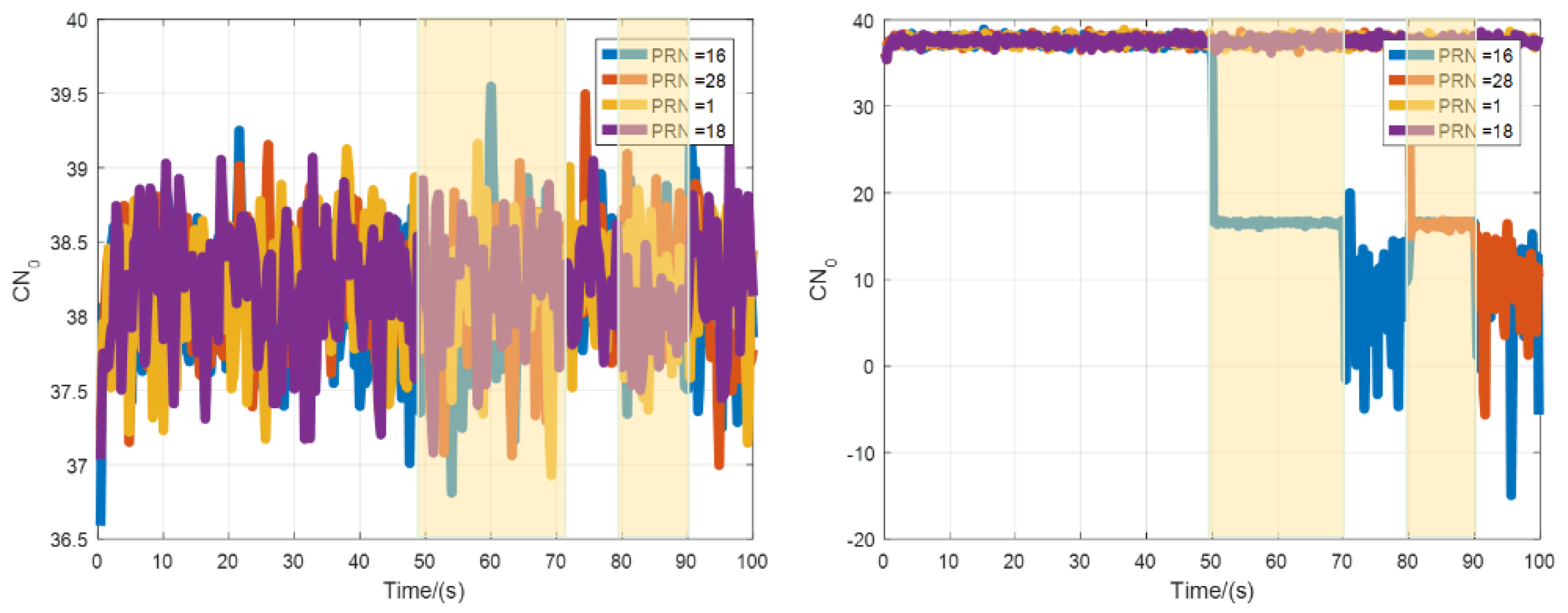
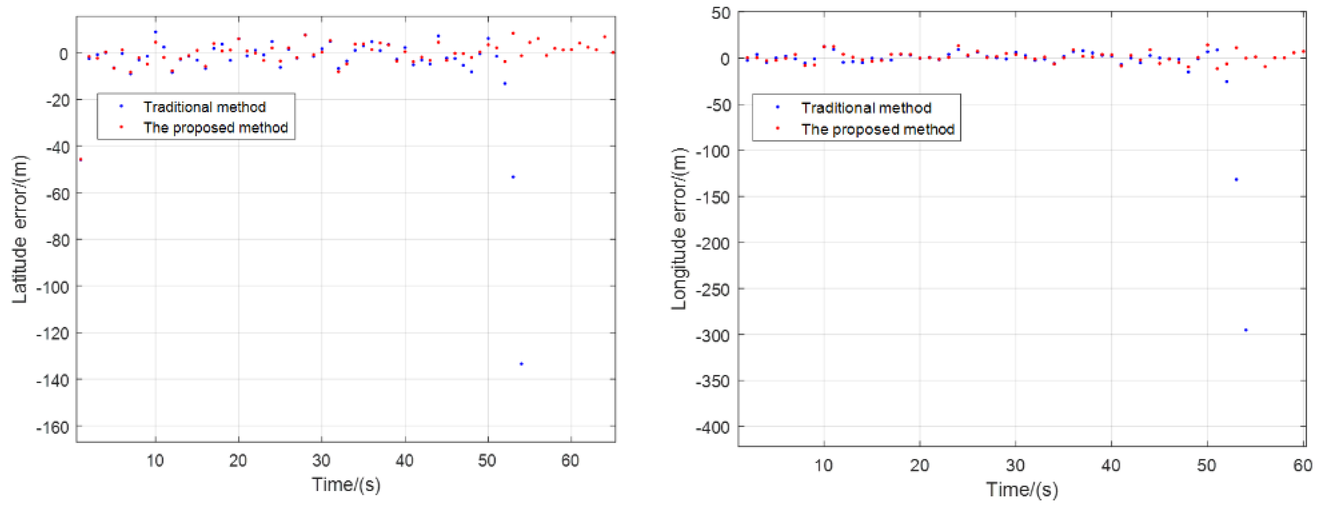
The signals with satellite numbers 16 and 28 are interrupted for different time periods. Figure 8 shows the signal mean square value of the prompt IQ branch. In the corresponding signal interruption interval, the value of the traditional method is obviously reduced, and the Doppler frequency shift is also abrupt in Figure 9. The proposed method corrects the code loop and the carrier tracking loop through the pseudo-range and pseudo-range rate fed back by the navigation solution module, and maintains the same accuracy as when the signal is visible. The C/N0 values of different channels of satellite signals are presented in Figure 10. In the absence of a signal, the C/N0 of the traditional tracking method drops rapidly, and cannot be restored when the signal returns to normal. The C/N0 of the proposed method basically remains stable. This is precisely because the channels of the traditional method are independent of each other and cannot realize the sharing and assistance of information, which causes the signal to easily lose lock. The proposed method uses the navigation filter module to unify the code phase error and the carrier frequency error as the measurement, and performs the filter estimation, which can realize the complementarity between the channels and improve the stability and accuracy of the system navigation and positioning. This can also be observed in Figure 11. After 50 s, due to the influence of signal interruption, the positioning results calculated by traditional methods gradually diverge, or even cannot be completed. The proposed method can still maintain the same positioning accuracy at the time when the satellite signal is available, which also illustrates the effectiveness and superiority of the proposed method.
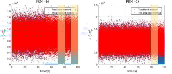
Figure 8.
The signal mean square value of the prompt IQ branch.
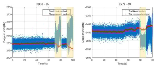
Figure 9.
The Doppler shift values of satellite signals (PRN =16,28).

Figure 10.
The C/N0 values of different channels of satellite signals.
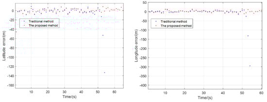
Figure 11.
Comparison results of horizontal position error in interference occasions.
4. Discussion and Conclusions
This paper designs an adaptive cascaded vector tracking loop to improve the stability and accuracy of the GNSS receiver in case of partial outage and limited satellites’ availability. First, in the signal tracking module, the KF is used to estimate the code phase error, carrier phase error, and carrier frequency error. Then, in the navigation solution module, the filtered output code phase error and carrier frequency error are converted into pseudo-range error and pseudo-range rate error, as the measurement signal of the EKF, and the feedback correction loop NCO is estimated through the navigation filter. Further, online adjustment of the measurement noise covariance matrix and the process noise covariance matrix are performed through the signal C/N0 and the innovation sequence, respectively. The vehicle test results show that, when the satellite is in good condition, the positioning result of the proposed method is slightly superior to the traditional method in terms of stability and accuracy. When the satellite signal is blocked or insufficient, the proposed method can still maintain high-quality positioning results, but the traditional method has failed. The proposed method in this paper provides a new idea for the practical application of the GNSS receiver signal tracking method. The next key task is to consider the multi-sensor fusion technology, and further improve the positioning accuracy and robustness of GNSS satellite signals in complex environments when assisted by external information, such as INS, Visual Odometer, 3D-Map, etc.
Author Contributions
Conceptualization, B.Z. and Q.W.; methodology R.Z.; software, L.W.; validation, B.Z., Q.W. and H.Y.; formal analysis, F.J.; investigation, B.Z.; resources, R.Z; data curation, Q.W.; writing—original draft preparation, H.Y.; writing—review and editing, B.Z.; visualization, Q.W.; supervision, L.W.; project administration, R.Z.; funding acquisition, Q.W. All authors have read and agreed to the published version of the manuscript.
Funding
This research was funded by the National Key R&D Program of China, grant number 2018YFB1702500.
Data Availability Statement
Restrictions apply to the availability of these data. Data were obtained from the Department of Precision Instrument and are available from the authors with the permission of B.Z. and Q.W.
Acknowledgments
I would like to express my gratitude to all those who helped me during the writing of this thesis. A special acknowledgement should be shown to Rong Zhang and Lixin Wang, from whose valuable suggestions I benefited greatly. I am particularly indebted to Bin Zhou and Qi Wei, and who gave me kind encouragement and supervised the work all through my writing. I wish to extend my thanks to Feng Ji who helped design the experiments finally.
Conflicts of Interest
The authors declare no conflict of interest.
References
- Xu, B.; Hsu, L.T. Open-source MATLAB Code for GPS Vector Tracking on a Software-defined Receiver. GPS Solut. 2019, 23, 1–9. [Google Scholar] [CrossRef]
- Won, J.H.; Eissfeller, B. A Tuning Method Based on Signal-to-noise Power Ratio for Adaptive PLL and its Relationship with Equivalent Noise Bandwidth. IEEE Commun. Lett. 2013, 17, 393–396. [Google Scholar] [CrossRef]
- O’Driscoll, C.; Petovello, M.G.; Lachapelle, G. Choosing the Coherent Integration Time for Kalman Filter-based Carrier-phase Tracking of GNSS Signals. GPS Solut. 2011, 15, 345–356. [Google Scholar] [CrossRef]
- Miao, Z.-Y.; Lv, Y.-L.; Xu, D.-J.; Shen, F.; Pang, S.-W. Analysis of a Variational Bayesian Adaptive Cubature Kalman Filter Tracking Loop for High Dynamic Conditions. GPS Solut. 2017, 21, 111–122. [Google Scholar] [CrossRef]
- Kim, K.H.; Jee, G.I.; Im, S.H. Adaptive Vector-tracking Loop for Low-quality GPS Signals. Int. J. Control Autom. Syst. 2011, 9, 709–715. [Google Scholar]
- Cheng, Y.; Chang, Q. A Carrier Tracking Loop Using Adaptive Strong Tracking Kalman Filter in GNSS Receivers. IEEE Commun. Lett. 2020, 24, 2903–2907. [Google Scholar]
- Jiang, R.; Wang, K.; Liu, S.; Li, Y. Performance Analysis of a Kalman Filter Carrier Phase Tracking Loop. GPS Solut. 2017, 21, 551–559. [Google Scholar] [CrossRef]
- Tang, X.; Falco, G.; Falletti, E.; Presti, L.L. Theoretical Analysis and Tuning Criteria of the Kalman Filter-based Tracking Loop. GPS Solut. 2015, 19, 489–503. [Google Scholar] [CrossRef]
- Petovello, M.G.; Lachapelle, G. Comparison of Vector-Based Software Receiver Implementations with Application to Ultra-Tight GPS/INS Integration. In Proceedings of the International Technical Meeting of the Satellite Division, Fort Worth, TX, USA, 26–29 September 2006; ION: Manassas, VA, USA; pp. 1–10. [Google Scholar]
- Won, J.H.; Dotterbock, D.; Eissfeller, B. Performance Comparison of Different Forms of Kalman Filter Approaches for a Vector-Based GNSS Signal Tracking Loop. Navigation 2010, 57, 185–199. [Google Scholar] [CrossRef]
- Won, J.H.; Pany, T.; Eissfeller, B. Characteristics of Kalman Filters for GNSS Signal Tracking Loop. IEEE Trans. Aerosp. Electron. Syst. 2012, 48, 3671–3681. [Google Scholar] [CrossRef]
- Xu, R.; Liu, Z.; Chen, W. Improved FLL-assisted PLL with In-phase Pre-filtering to Mitigate Amplitude Scintillation Effects. GPS Solut. 2015, 19, 263–276. [Google Scholar] [CrossRef]
- Sun, Z.; Wang, X.; Feng, S.; Che, H.; Zhang, J. Design of an Adaptive GPS Vector Tracking Loop with the Detection and Isolation of Contaminated Channels. GPS Solut. 2017, 21, 701–713. [Google Scholar] [CrossRef]
- Lashley, M.; Bevly, D.M.; Hung, J.Y. Impact of Carrier to Noise Power Density, Platform Dynamics, and IMU Quality on Deeply Integrated Navigation. In Proceedings of the ION Position, Location and Navigation Symposium, Monterey, CA, USA, 5–8 May 2008; IEEE: Piscataway, NJ, USA; pp. 9–16. [Google Scholar]
- Lashley, M.; Bevly, D. Comparison of Adaptive Estimation Techniques for Vector Delay/Frequency Tracking. In Proceedings of the Guidance, Navigation and Control Conference and Exhibit, Honolulu, HI, USA, 18–21 August 2008; AIAA: Reston, VA, USA; p. 7474. [Google Scholar]
- Dou, J.; Xu, B.; Dou, L. Performance Assessment of GNSS Scalar and Vector Frequency Tracking Loops. Optik 2020, 202, 163552. [Google Scholar] [CrossRef]
- Dou, J.; Xu, B.; Dou, L. An Intelligent Joint Filter for Vector Tracking Loop Considering Noise Interference. Optik 2020, 219, 164984. [Google Scholar] [CrossRef]
- Marçal, J.; Nunes, F.; Sousa, F.M. Performance of a Scintillation Robust Vector Tracking for GNSS Carrier Phase Signals. In Proceedings of the Workshop on Satellite Navigation Technologies and European Workshop on GNSS Signals and Signal Processing, Noordwijk, The Netherlands, 14–16 December 2016; IEEE: Piscataway, NJ, USA; pp. 1–8. [Google Scholar]
- Marçal, J.; Nunes, F.; Sousa, F.M. Performance of an adaptive Partitioned Vector Tracking Algorithm with Real Scintillation Data. In Proceedings of the Workshop on Satellite Navigation Technologies and European Workshop on GNSS Signals and Signal Processing, Noordwijk, The Netherlands, 5–7 December 2018; IEEE: Piscataway, NJ, USA; pp. 1–8. [Google Scholar]
- Marçal, J.; Nunes, F. Robust Vector Tracking for GNSS Carrier Phase Signals. In Proceedings of the International Conference on Localization and GNSS, Barcelona, Spain, 28–30 June 2016; IEEE: Piscataway, NJ, USA; pp. 1–6. [Google Scholar]
- Lin, H.; Huang, Y.; Tang, X.; Xiao, Z.; Ou, G. Robust Multiple Update-rate Kalman Filter for New Generation Navigation Signals Carrier Tracking. GPS Solut. 2018, 22, 1–12. [Google Scholar]
- Tang, X.; Falco, G.; Falletti, E.; Presti, L.L. Complexity Reduction of the Kalman Filter-based Tracking Loops in GNSS Receivers. GPS Solut. 2017, 21, 685–699. [Google Scholar] [CrossRef]
- Yang, R.; Ling, K.-V.; Poh, E.-K.; Morton, Y. Generalized GNSS Signal Carrier Tracking: Part I—Modeling and Analysis. IEEE Trans. Aerosp. Electron. Syst. 2017, 53, 1781–1797. [Google Scholar] [CrossRef]
- Ziedan, N.I.; Garrison, J.L. Extended Kalman Filter-based Tracking of Weak GPS Signals under High Dynamic Conditions. In Proceedings of the International technical meeting of the satellite division of the Institute of Navigation, Long Beach, CA, USA, 21–24 September 2004; ION: Manassas, VA, USA; pp. 20–31. [Google Scholar]
- Bhattacharyya, S.; Gebre-Egziabher, D. Vector Loop RAIM in Nominal and GNSS-stressed Environments. IEEE Trans. Aerosp. Electron. Syst. 2014, 50, 1249–1268. [Google Scholar] [CrossRef]


Publisher’s Note: MDPI stays neutral with regard to jurisdictional claims in published maps and institutional affiliations. |
© 2021 by the authors. Licensee MDPI, Basel, Switzerland. This article is an open access article distributed under the terms and conditions of the Creative Commons Attribution (CC BY) license (https://creativecommons.org/licenses/by/4.0/).