A Multiscale Method for Road Network Extraction from High-Resolution SAR Images Based on Directional Decomposition and Regional Quality Evaluation

Abstract

Road network is an important part of modern transportation. For the demands of accurate road information in practical applications such as urban planning and disaster assessment, we propose a multiscale method to extract road network from high-resolution synthetic aperture radar (SAR) images, which consists of three stages: potential road area segmentation, preliminary network generation, and road network refinement. Multiscale analysis is implemented using an image pyramid framework together with a fixed-size filter. First, a directional road detector is designed to highlight road targets in feature response maps. Subsequently, adaptive fusion is performed independently at each image scale, followed by a threshold method to produce potential road maps. Then, binary maps are decomposed according to the obtained direction information. For each connected component (CC), quality evaluation is conducted to further distinguish road segments and polynomial curve fitting is adopted as a thinning method. Multiscale information fusion is realized through the weighted sum of road curves. Finally, tensor voting and spatial regularization are employed to generate the final road network. Experiments on three TerraSAR images demonstrate the effectiveness of the proposed algorithm to extract road network completely and correctly.

1. Introduction

Road networks are a type of typical geographic information that plays an essential role in various applications including urban planning, traffic control, disaster assessment, change detection, etc. [1,2,3,4]. However, road networks, mainly composed of asphalted pavement, evolve with changes in the city constantly and road information in cadastral databases needs periodical supplement and improvement. Manual marking to update the road network is costly in terms of human resources, with heavy workloads, and it is hard to reach real-time requirements such as emergency rescue in severe natural disasters. With the development of remote sensing, researchers have explored the extraction of road networks automatically from satellite images. Unfortunately, the commonly used optical remote sensing images are severely affected by weather. With all-day, all-weather, and high-resolution imaging capabilities, synthetic aperture radar (SAR) images have gained extensive attention and are popular in road extraction tasks. However, road network extraction from SAR images is still a challenging task due to the special side-view imaging mechanism, diversity road targets, and complex surroundings.

Among various reported methods, road network extraction algorithms consist of two stages in general, that is road element recognition and road network reconstruction. The purpose of the first stage is to highlight the road area and to discriminate road candidates. The second stage aims to discard redundant pixels and to fill the gaps to generate smooth and continuous road lines. With regard to road element recognition, local detectors such as ratio edge detector [5,6] and morphological line detector [7] are applied to extract road features. Moreover, direction [8], contrast [9], and some other spatial characteristics are considered to generate multiple road feature maps. After that, feature fusion [10,11] and threshold method [6] are adopted to distinguish road pixels from background pixels. With the rapid growth of deep learning, road segmentation based on deep fully convolutional neural networks has been developed [12]. For road network reconstruction, thinning and spatial optimization are two important parts. The thinning algorithm was employed on binary segmented road maps to extract road centerlines, in which morphological thinning is simple and fast to implement but sensitive to noise. Later, regression-based thinning methods [13,14] with noise robustness were proposed. In [15], boundary distance field and source distance field were generated via the fast marching method (FMM) algorithm, and then, branch backing-tracking method was employed to produce the initial road centerline. Commonly used methods for spatial optimization contain Markov random fields (MRFs) [6,9] and genetic algorithm [16]. In [17], the conditional random field (CRF) model was utilized to implement road network optimization in a Bayesian framework. Region growing [18,19] and parallel particle filter [20] were adopted to track road networks based on the automatically extracted seed points.

It has been well accepted that human vision is an inherently multiscale phenomenon [21]. We hope that a similar system can be installed in computers to automatically extract spatial information from different image scales. Thereupon, many algorithms derived from human visual were proposed, which can be regarded as a series of scaled filters or repeatedly used filter on different spatial scales. Recently, several multi-scale geometric analysis (MGA) [22] tools were developed and have been successfully applied in the field of image processing. In [23], shearlet was used to detect road edges from SAR images with strong speckle noise. With the ability to represent linear and curvilinear features, beamlet analysis was employed to extract guidance lines from the response map in [24]. As an efficient and convenient representation of image expression in multiple resolutions, image pyramid was originally designed for image compression and has been widely used in computer vision tasks including image registration [25], image fusion, and target detection [26].

In high-resolution SAR images, we suppose that road targets have the following characteristics. (1) Local uniformity: a road surface is at least locally homogeneous. Considering the low surface roughness and low permittivity [27], roads always appear as uniform dark areas. (2) Local directionality: the curvature of roads change slowly in a local area, which means that the adjacent road pixels usually have similar directions. (3) Continuity: roads are generally elongated structures with a certain width and seldom shown as small separate fragments. The combination of these features can be rarely found in other objects; thus, we are dedicated to making full use of these features for a promising extraction result.

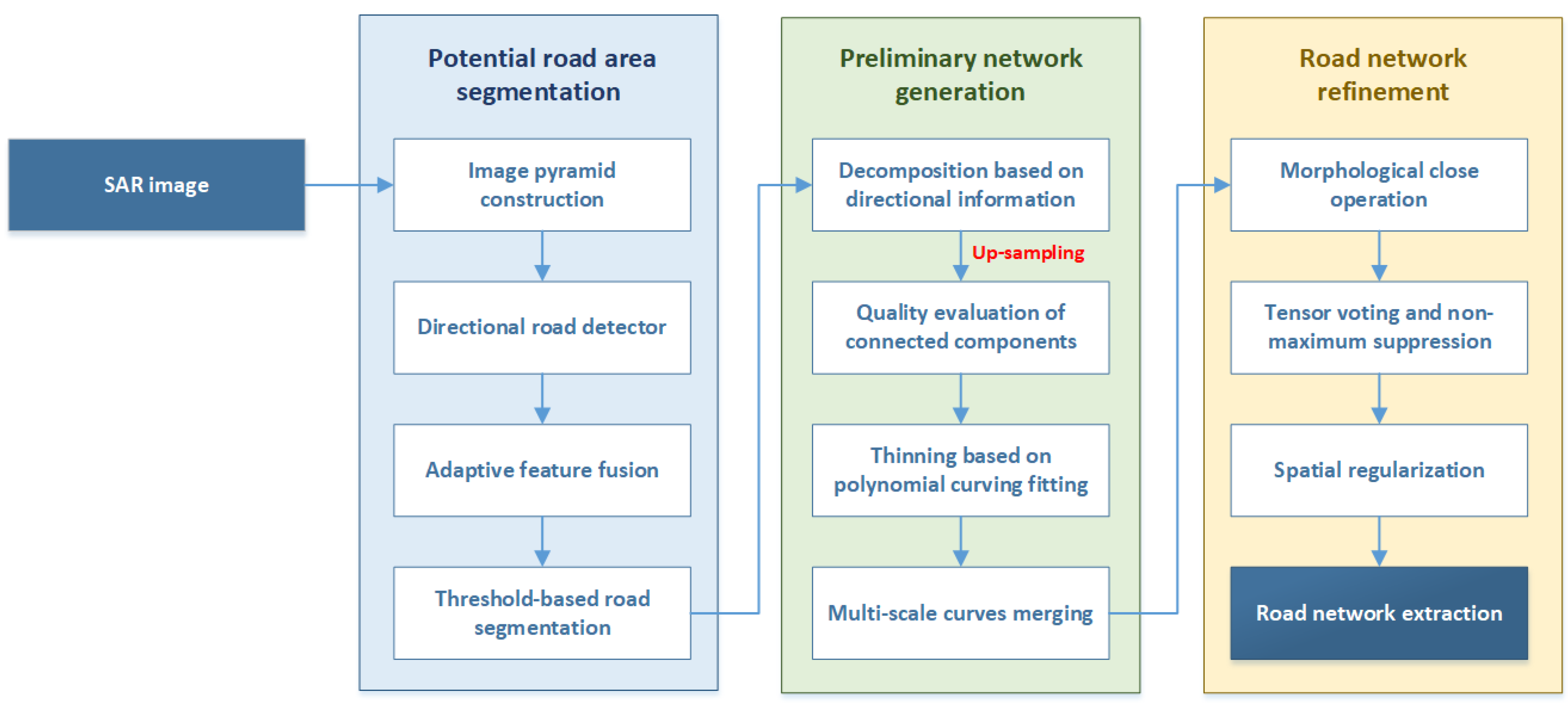
In this paper, we propose a road network extraction algorithm under a multiscale framework for high-resolution SAR images. Our method consists of three stages: potential road area segmentation, preliminary network generation, and road network refinement. The first stage corresponds to the road element recognition mentioned above. To capture road targets with different widths, an image pyramid is constructed together with a fixed filter for multiscale analysis. A directional road detector with slender detection templates is developed as the fixed-size filter to extract road features including radiance, texture, direction, and invariant moment. Then, adaptive fusion is performed to integrate the feature maps of each scale separately, following by threshold segmentation to obtain the binary road maps. In preliminary network generation, to overcome the difficulty in fitting road targets with irregular structures, image decomposition is firstly conducted on multiscale binary road maps according to the direction map generated in the first stage. To further select regions that are likely to be road segments, we evaluate the quality of each connected component (CC) based on the combination of four predefined indicators. It is worth noting that multiscale image layers are upsampled to the input image size to ensure the evaluation fairness. After that, polynomial curve fitting is performed as a thinning method on all CCs. Based on the results of the evaluation function, the weighted sum of curves realizes multiscale information fusion and produces the preliminary road network. Road network refinement aims to ensure the smoothness and continuity of a network. Tensor voting (TV) and spatial regularization are implemented to obtain the final road network extraction result. Qualitative and quantitive analyses on extracted results of three TerraSAR images prove the validity of our method.

The remainder of this paper is organized as follows. Details of the road network extraction method are described in Section 2. Parameter analysis and experiment results are shown in Section 3. Comparisons with related methods and discussions on algorithm performance are provided in Section 4. Finally, conclusions are given in Section 5.

2. Method

In this section, we introduce a multiscale road network extraction method for high-resolution SAR images. The flowchart of the proposed algorithm is displayed in Figure 1. Details of the aforementioned steps are presented in the following subsections.

2.1. Image Pyramid Construction

The width of lanes varies with the road level. Generally speaking, urban lanes are wider than rural ones. Along with the change in the number of lanes, road widths vary significantly in remote sensing images. At the same time, image resolution also has great influence on the road pixel width. In low-resolution images, road targets appear as curves approximately, while in high-resolution images, road targets present as elongate areas with a certain width. In [18], road width is essential to setting appropriate filter parameters and obtaining satisfying extraction results. However, in actual road network extraction task, road width is always unknowable. The widely used D1D2 road detector [28] adopts multi-direction and multi-size detection templates, and the maximum response value is obtained when the template is fully matched with the width and direction of the road. It has a high time complexity and low operation efficiency. In this paper, we conduct multiscale analysis based on the pyramid model to overcome the unpredictability and diversity of road width and to improve the efficiency of road detection.

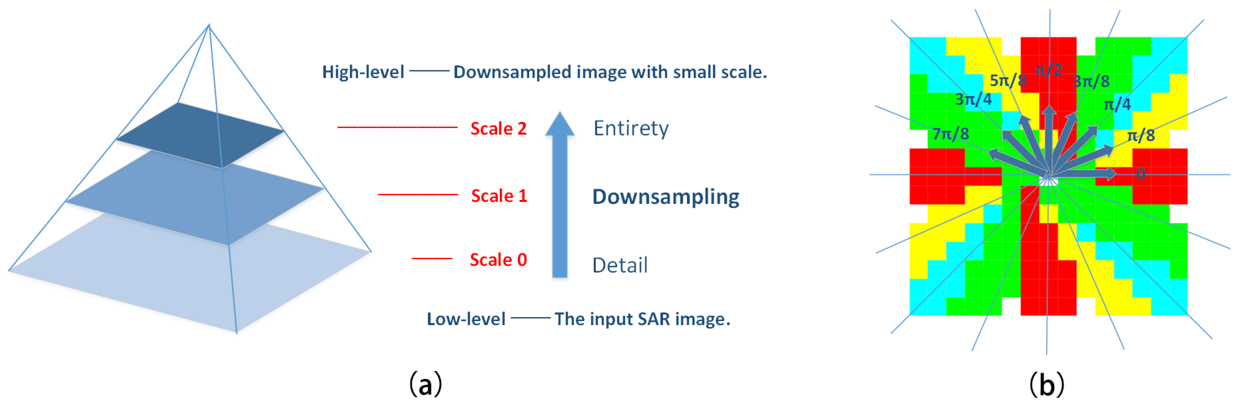
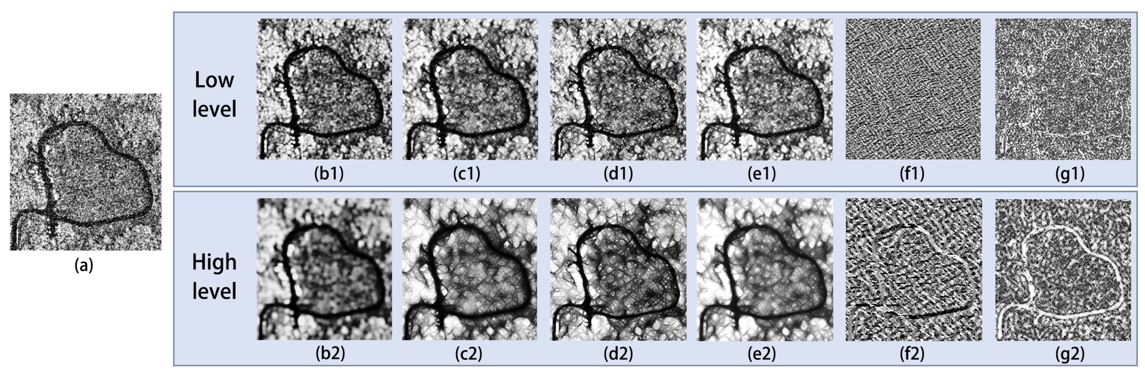
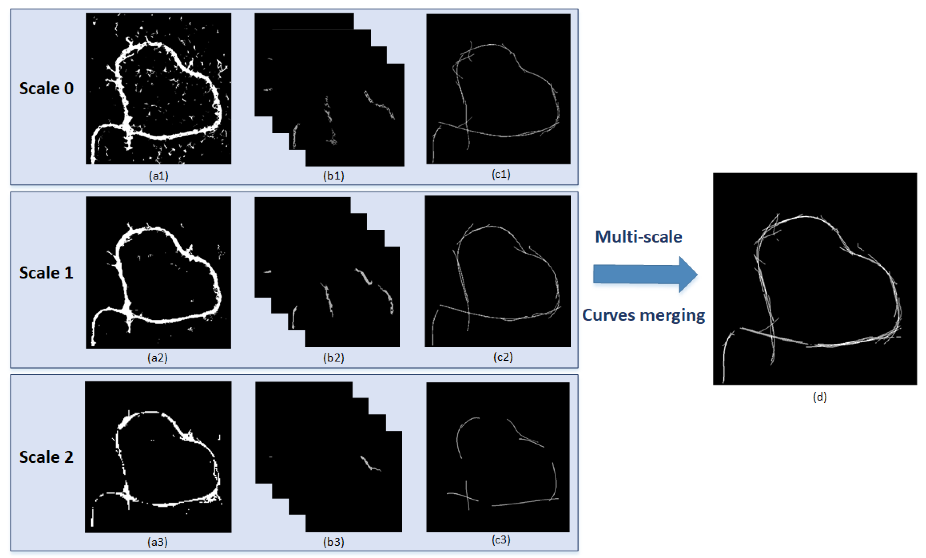
The pyramid model is shown in Figure 2a. The image size is reduced by half with each downsampling operation from the bottom up. Scale 0 corresponds to the input SAR image, which depicts image details and facilitates the extraction of narrow roads. In the high-level images, features of narrow roads gradually disappear while features of wide roads are retained, which benefit the extraction of the basic trends of roads and emphasize the location of main roads. Empirically, we find that three image scales are enough for the road network extraction task. The steps of multiscale analysis are as follows. Firstly, road area segmentation and directional-based image decomposition are performed on various image scales independently. After that, the decomposed image layers with different sizes are interpolated to the original image size through the nearest neighbor interpolation algorithm. Then, regional quality evaluation and the thinning operation are carried out. Finally, multiscale information fusion is implemented by the combination of weighted curve images.

2.2. Directional Road Detector

Affected by the surroundings and speckle noise in SAR images, the mere use of intensity information is insufficient to segment the complete road area. Therefore, a directional road detector is designed according to the road features, aiming at identifying road area from the output response maps.

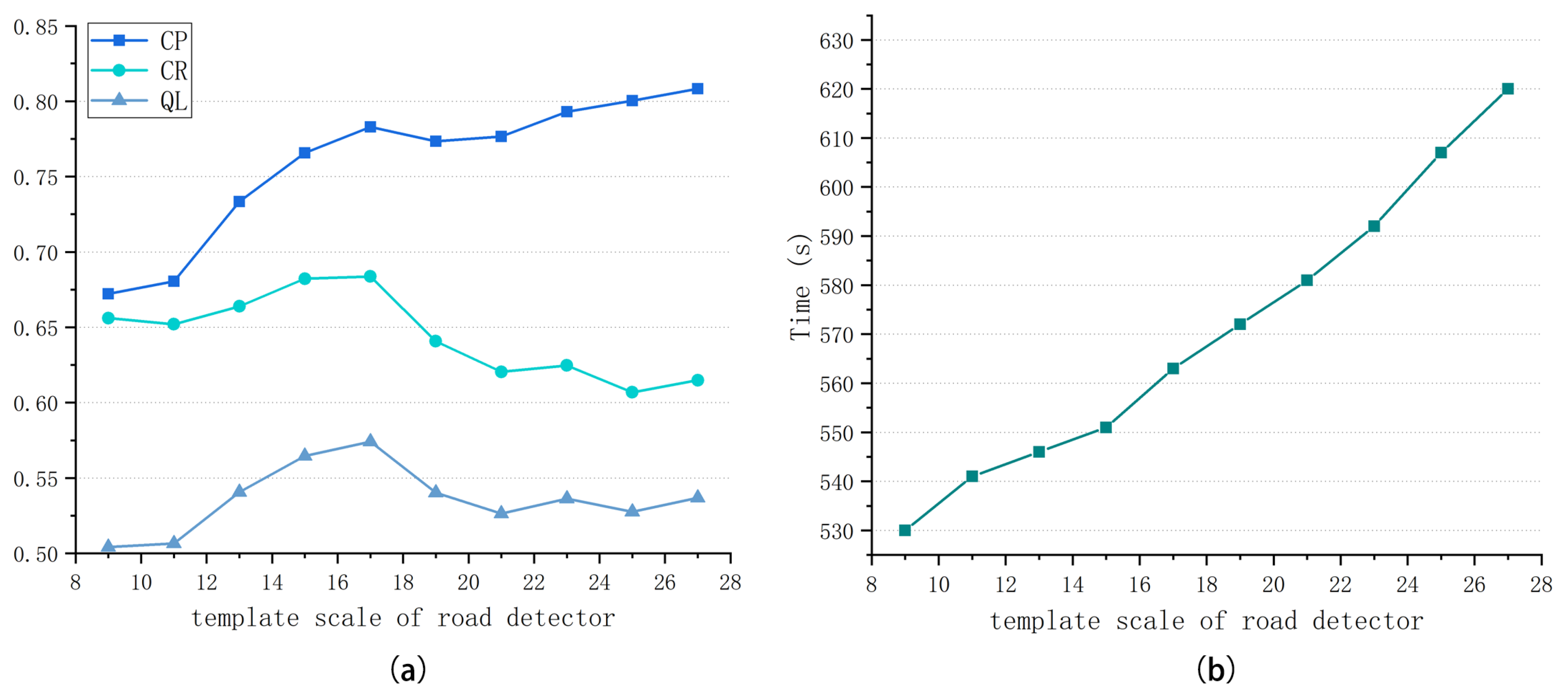
Eight matrices with fixed size and different directions are used as detection templates, as shown in Figure 2b. The direction of the eight templates satisfies $\theta \in \{0,\frac{\pi }{8},\frac{\pi }{4},\frac{3\pi }{8},\frac{\pi }{2},\frac{5\pi }{8},\frac{3\pi }{4},\frac{7\pi }{8}\}$. To fit the elongated structure of road targets, detection is conducted in a slender rectangular area. Road targets show definite directionality; thus, we conduct detection in multiple directions and retain the direction information of the optimal response. Based on the multi-scale framework, a fixed-size template can meet the demands of extracting roads with different widths. An appropriate size is carefully selected for detection templates according to the image resolution. If the size is too small, the response map will be seriously affected by noise and fail to highlight road area. If the size is too large, it will neglect some road details and bring about heavy calculation burdens.

Firstly, we calculate the statistical characteristics of eight rectangular regions centered on pixel p. The mean and variance of region k are denoted as ${\mu }_k$ and ${\sigma }_k$, respectively. Then, we use two different operators to generate the radiance response map and texture response map, which can distinguish dark uniform areas from the original SAR images. As is mentioned above, roads appear as dark and elongated regions in SAR images. A small value of ${\mu }_k$ indicates a high probability of region k to be located in road areas [9]. Therefore, the minimum mean value among eight templates is selected as the radiance response $m\left(p\right)$ of pixel p, which can be expressed as

$$m\left(p\right)=min\left\{{\mu }_k\right\},k=1,2,\cdots ,8$$

(1)

The corresponding direction is denoted as $A\left(p\right)$, that is

$$A\left(p\right)=arg\underset{{\theta }_k}{min}\left\{{\mu }_k\right\},k=1,2,\cdots ,8$$

(2)

The multiplicative noise in SAR image has more influence on the brighter area than the darker one. Beyond that, road targets have local uniformity, which appear as homogenous regions with low grayscale. Obviously, a small value of ${\sigma }_k$ means a high probability of region k being located in road areas. We select the minimum value of ${\sigma }_k$ among eight templates as the texture response $s\left(p\right)$ of pixel p, which is written as

$$s\left(p\right)=min\left\{{\sigma }_k\right\},k=1,2,\cdots ,8$$

(3)

Due to the limitation of the slender neighborhood, the slight changes along a certain orientation are obviously reflected in directional road response maps. As shown in Figure 3c,d, the dark streaks in non-road areas are disorderly and bring disturbance to road area segmentation. In order to facilitate the road extraction task, a fast and effective method is employed to produce a feature map with smooth change within each region and significant differences between regions. As known, the moment is a statistical characteristic of random variables and can describe various geometric features of a given image. For a two-dimensional digital image, the $p+q$-order original moment is defined as

$$m_{pq}=\sum _{x=1}^R\sum _{y=1}^C{x}^p{y}^{q}I(x,y)$$

(4)

where R and C stand for the number of rows and columns, respectively. The central moment of the $p+q$-order is given by

$${\mu }_{pq}=\sum _{x=1}^R\sum _{y=1}^C{(x-\overline{x})}^p{(y-\overline{y})}^{q}I(x,y)$$

(5)

where $\overline{x}=m_{10}/m_{00},\overline{y}=m_{01}/m_{00}$. The normalized central moment of the $p+q$-order can be written as

$${\eta }_{pq}=\frac{{\mu }_{pq}}{{\mu }_{00}^{\rho }},\rho =\frac{p+q}{2}+1$$

(6)

The first invariant moment in [29] is adopted to generate an invariant moment feature map in this paper, which is expressed as

$$M1={\eta }_{20}+{\eta }_{02}$$

(7)

2.3. Adaptive Feature Fusion

Considering the complementarity of the radiance response map, texture response map, and invariant moment feature map, we adopt the adaptive multifeature fusion method in [30] to separately combine the extracted information from different image scales. At a certain image scale, three feature maps are normalized to $\left[0,1\right]$. It should be noted that road targets have large values in the invariant moment feature map, which is inconsistent with the other two feature maps. Thus, inverse operation is performed on the normalized invariant moment feature map. Then, three segmentation thresholds generated by OSTU method [31] should be transformed to the same location before fusion. The preliminary road segmented map is obtained after the threshold segmentation of the fusion map.

The directional road detector is capable of dividing uniform dark areas from the original SAR images. However, due to the similarity of features, some regions are misclassified into road targets, such as shadows, rivers, and squares. Fortunately, they are not exactly the same as road targets in SAR images. In the subsequent processing, we will eliminate the discrete regions from potential road areas through the continuity of road targets and exclude the interference of regions with low shape compactness (such as squares) according to the regional directivity.

2.4. Binary Image Decomposition Based on Directional Information

Practically, roads are arranged in a crisscross pattern with diverse distributions. CCs in the binary segmented maps often have irregular and complex shapes resulting in difficulty fitting the connected regions directly. However, road targets have local directionality, which assumes that the direction of the road within the local area remains unchanged. Inspired by the idea of direction feature grouping [32], we decompose the road binary segmented map with the help of direction information.

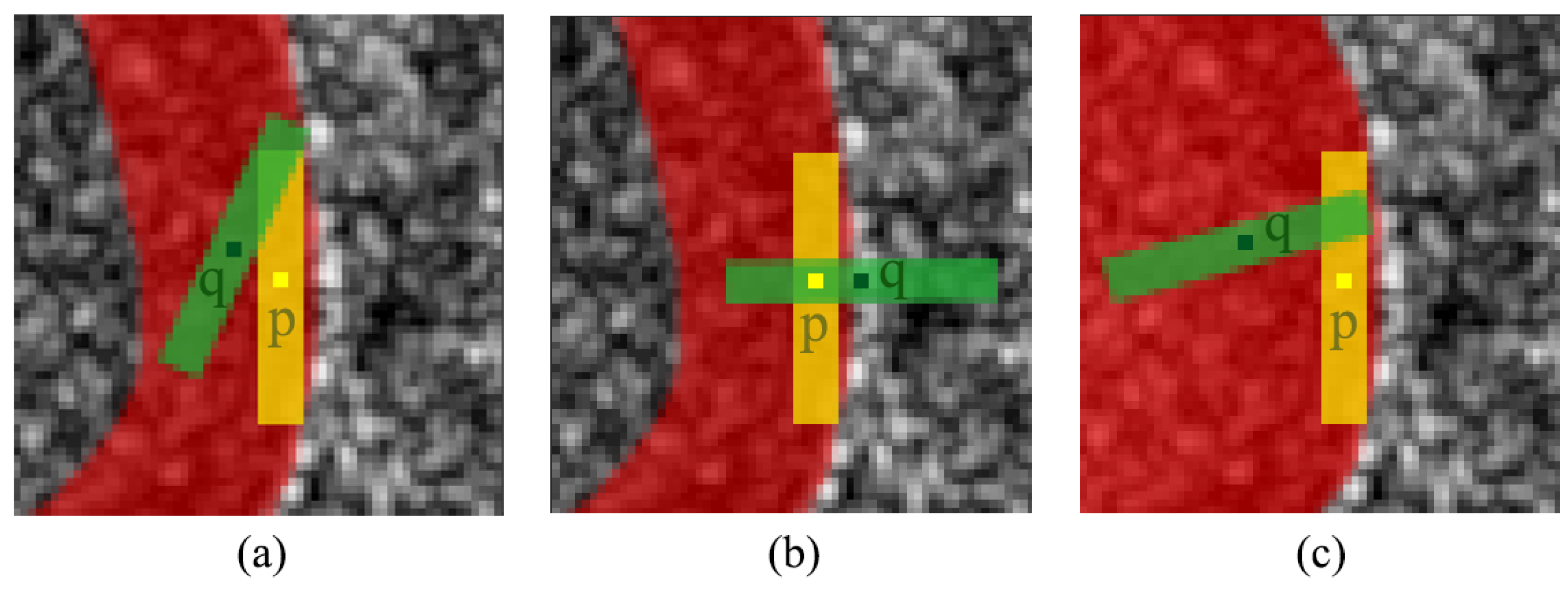
In this paper, the direction map A acquired in Section 2.2 serves as the guidance of binary map decomposition. Figure 4 is used to discuss the relationship between the value of A and road position. We suppose that the potential road area is painted in red, wherein the yellow pixel p is located in the potential road area close to the road edge and the green pixel q is in the neighborhood of pixel p. The rectangular regions along the directions of $A\left(p\right)$ and $A\left(q\right)$ are shown in light yellow and light green, respectively. The direction of $A\left(p\right)$ is parallel to the road edge. In Figure 4a, pixel q is located in the road area and the value of $A\left(q\right)$ is similar to $A\left(p\right)$. Pixel q in Figure 4b is outside the road area, meanwhile the direction of A(q) is perpendicular to the road edge. In Figure 4c, the green pixel q is also located in the potential road area. However, the shape of the red area is incongruent with the elongate structure of road targets, leading to the relatively random direction of pixel $A\left(q\right)$. To sum up, the value of A changes smoothly in the elongated road area while the value of A changes abruptly when crossing the road edge. In the broad dark area, the value of A is unpredictable. In the non-potential road area, the value of A changes irregularly under the influence of complex environment. Therefore, the direction map A is taken as a reference of direction-based image decomposition. In the decomposed image, road targets present as long and narrow CCs whereas the dark area with low compactness appears as discrete points.

In order to prevent CCs from being too scattered in decomposed layers and from reducing the complexity of image combination, eight values in the direction map A are divided into four groups according to the direction similarity. That is, $G_1=\{0,\frac{7\pi }{8}\}$, $G_2=\{\frac{\pi }{8},\frac{\pi }{4}\}$, $G_3=\{\frac{3\pi }{8},\frac{\pi }{2}\}$, and $G_4=\{\frac{5\pi }{8},\frac{3\pi }{4}\}$. Image decomposition can be written as follows:

$$B{W}_i=BW\&A_{G_i},i=1,2,3,4$$

(8)

$$A_{G_i}\left(p\right)=\left\{\begin{array}{cc}1,\hfill & ifA\left(p\right)\in G_i\hfill \\ 0,\hfill & else\hfill \end{array}\right.$$

(9)

where & represents the per-pixel logical “AND” operation, $BW$ is the potential road map obtained by threshold segmentation, $A_{G_i}$ marks the positions that have similar directions to $G_i$, and $B{W}_i$ represents the decomposed image layer k. Clearly, the direction of CCs in image layer $B{W}_i$ mostly remains consistent with the direction guidance $G_i$.

Due to the influence of speckle noise, road width, shelter, and some other factors, there exist multiple fragments and dense point sets in the decomposed layers. The dense point sets are formed for two reasons. Firstly, the direction of road where the point set is located is halfway between two adjacent decomposition directions, thus, the road area is decomposed into two parts forming two complementary discrete point sets. Secondly, the distribution of direction map A is highly random in dark regions with low compactness, resulting in discrete point sets after image decomposition. It should be noted that road targets tend to form discrete point sets in decomposed layers when the road width is about equal to or greater than the length of a detection template. In a low-level image, narrow roads show regularity while wide roads show high randomness in direction map A. In high-level image, the width of roads is reduced to ensure that the largest width is significantly smaller than the length of the detection template and that the regularity of wide roads emerges in direction map A.

To connect the dense point sets into a whole, a morphological CLOSE operation is performed on the decomposed layers. The operation not only improves the continuity of the road area but also benefits the following work, making it easier to fit each CC to a straight line or curve. Whether a point set is located in a road area will be discussed in the next subsection. Subsequently, all decomposed layers with multiple scales are upsampled to the original image scale through the nearest neighbor interpolation to ensure the fairness that regional quality assessment is carried out at the same scale.

2.5. Quality Evaluation on Connected Components

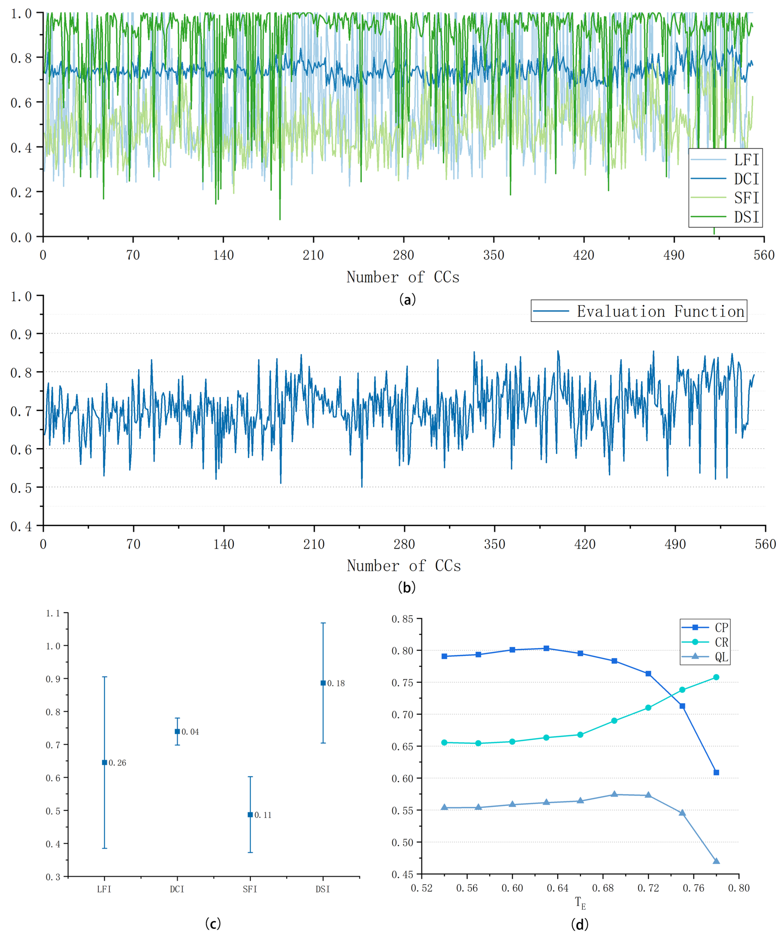
After binary image decomposition, each layer contains multiple CCs with different areas, directions, and shapes. CCs involve both multiscale road segments and the wrongly divided dark regions. According to the characteristics of the road targets, we set several indexes to evaluate the quality of CCs. The value of evaluation function is correlated with the probability that the current CC is located in a road area. On the one hand, we can select road segments at the appropriate scale and further eliminate the non-road segments resulting from inaccurate segmentation. On the other hand, different weights can be given to CCs during image merging, providing meaningful information for global network optimization.

The first indicator is Linearity Feature Index (LFI). Ideally, road targets appear as continuous strips in decomposed image layers. The straighter and longer the shape of the area, the higher probability it is a part of a road. Referring to the LFIe index in [33] ($LFIe=\frac{L_e}{W_e}$), we define the measure of the linearity of CC in this paper:

$$LFI=\frac{1}{T{H}_L}min(\frac{L_e}{W_e},T{H}_L)$$

(10)

where $L_e$ and $W_e$ represent the length of the long axis and the short axis of the ellipse for which the standard second-order central moment is the same as the CC. $T{H}_L$ is the upper limit of $LFIe$. Setting the threshold is convenient for normalization and comprehensive assessment with other indexes. We believe that CCs with $LFIe$ index greater than 5 have satisfied the shape characteristics of road targets. Thus, the value of $T{H}_L$ is set as 5 in our method.

The second indicator is the Directional Consistency Index (DCI). The locally statistical directivity D is defined by the cosine sum of the intersection angles between the direction of center pixel and neighborhood pixels in the direction map A:

$$D\left(p\right)=\frac{1}{{\gamma }_D}\sum _{q\in N\left(p\right)}cos\left(min(\left|A\left(p\right)-A\left(q\right)\right|,\pi -\left|A\left(p\right)-A\left(q\right)\right|)\right)$$

(11)

where ${\gamma }_D$ is a normalization factor and $\left|·\right|$ is the absolute value operation. A large value of D indicates the high similarity of pixel directions in the neighborhood and a high probability of being located in the elongated road area. The mean value of D is regulated as a directional consistency of CC:

$$\mathrm{DCI}=\frac{{\sum }_{p\in \Omega }{D}_p}{N_{\Omega }}$$

(12)

where $N_{\Omega }$ counts the number of pixels in connected region $\Omega$. A high DCI value means that the current CC stands a good chance of being a road area. Dense point sets in the road area have similar directions as their neighborhoods, leading to a high DCI value. In contrast, the point sets in the dark region with low compactness usually have different directions with their neighborhoods, resulting in a low value of DCI.

The third indicator is the Solidity Feature Index (SFI). If the road width does not match the image scale, wide roads will appear as small aggregated fragments or regions with irregular boundaries and large holes. If processed at an appropriate scale, road targets will appear as solid strip regions in decomposed layers. Therefore, solidity is employed to select CCs generated at a proper image scale, which is defined as the area ratio between the region and its minimum convex polygon:

$$\mathrm{SFI}=\frac{N_{\Omega }}{N_{{\Omega }_c}}$$

(13)

where $N_{{\Omega }_c}$ counts the number of pixels in the minimum convex polygon of CC. A high SFI value represents that the current image scale is appropriate for the road width and that the CC makes a great contribution to the road network generation.

The fourth indicator is the direction similarity between CC and decomposition guidance (DSI). Since the binary image is decomposed based on direction information, the pixels have the same direction in each decomposed layer. Therefore, the direction of CC is likely to be consistent with the corresponding decomposition guidance. DSI is regulated as follows:

$$\mathrm{DSI}=cos\left(min(\left|D_e-D_G\right|,\pi -\left|D_e-D_G\right|)\right)$$

(14)

where $D_e$ represents the intersection angle between the long axis of the ellipse for which the standard second-order central moment is the same as the CC and the horizontal direction. $D_G$ represents the main direction of the decomposition, which is the average value of the directions in group $G_i$. In this paper, the four main directions are $\frac{3}{16\pi }$, $\frac{7}{16\pi }$, $\frac{11}{16\pi }$, and $\frac{15}{16\pi }$. A larger DSI value indicates a higher credibility of the current region in the road network composition.

To comprehensively access each CC, we combine four indicators and define the evaluation function as follows:

$$E=\frac{{\alpha }_L·\mathrm{LFI}+{\alpha }_C·\mathrm{DCI}+{\alpha }_S·\mathrm{SFI}+{\alpha }_D·\mathrm{DSI}}{{\alpha }_L+{\alpha }_C+{\alpha }_S+{\alpha }_D}$$

(15)

where ${\alpha }_L$, ${\alpha }_C$, ${\alpha }_S$, and ${\alpha }_D$ are weight parameters, which can be used to adjust the importance of four indexes in quality evaluation. The values of LFI, DCI, SFI, and DSI have been normalized in the previous formulas; thus, the value of E is between 0 and 1. A high value of E means a high quality of CC, which has a great possibility to be a road region and has a large weight in the image merging process.

2.6. Thinning Based on Polynomial Curve Fitting and Preliminary Road Network Generation

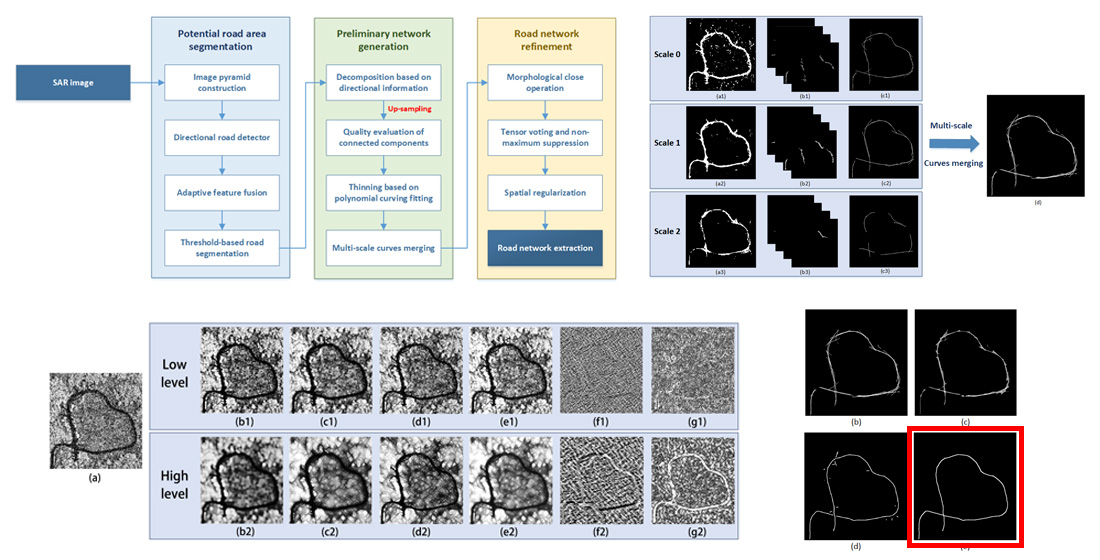
A thinning operation is necessary for the purpose of extracting the centerline from the binary segmented map. In this paper, thinning is firstly conducted on each CC in upsampled image layers, and then, we integrate all curves by weighted summation. A road centerline presents as straight line or smooth curve in the actual scene. In order to obtain accurate road networks, the polynomial curve fitting method [32] is adopted to conduct thinning operation on each CC, in which the order of polynomial is set as 3.

After that, thinned image layers generated by different image scales are merged to produced a complete road network. Image merging is the weighted sum of the fitting curves, which can be written as follows:

$$B{W}^{{}^{\prime }}=\sum _i\sum _{\Omega }B{W}_{i,\Omega }^{{}^{\prime }}·E_{\Omega }$$

(16)

where $B{W}^{{}^{\prime }}$ is the preliminary road network, $B{W}_{i,\Omega }^{{}^{\prime }}$ is the thinned binary map of region $\Omega$ in image layer i, and the evaluation result $E_{\Omega }$ of region $\Omega$ is the weight coefficient in image merging. The preliminary road network is a simple stack of several weighted curves, which contains redundant duplicates, protruded lines, and unconnected gaps, as shown in Figure 5d.

2.7. Tensor Voting and Non-Maximum Suppression

Tensor voting [34] has been widely used for thinning and refinement in the task of road network extraction, which also shows strong robustness on SAR images. Relying on tensor representation and data communication between adjacent tensors, salient information can be effectively perceived from sparse and noisy two-dimensional images. The time-consumption of tensor voting is positively correlated with the sparsity of the input image. In this paper, morphological CLOSE operation is firstly performed on the preliminary network to fill the blank between adjacent curves and to construct a connected region; then, tensor voting is conducted on the consolidated road network, which greatly reduces the runtime compared with tensor voting conducted on the binary segmented map [13,33]. Meanwhile, the consolidated road network has a clearer structure and definitely produces more accurate results than the segmented map.

In the framework of tensor voting, the input information is some point clouds called tokens. Each token is encoded as a symmetric tensor, and then, a tensor field is generated. For a two-dimensional image, the input is sparse pixels that only contain location and amplitude information. Firstly, each pixel is transformed into a second-order anisotropic tensor [35]. Each tensor can be denoted as a linear combination of eigenvectors and eigenvalues:

$$T={\lambda }_1{e}_1{e}_1^T+{\lambda }_2{e}_2{e}_2^T=\left[\begin{array}{cc}{e}_1& e_2\end{array}\right]\left[\begin{array}{cc}{\lambda }_1& 0\\ 0& {\lambda }_2\end{array}\right]\left[\begin{array}{c}{e}_1^T\\ e_2^T\end{array}\right]$$

(17)

where ${\lambda }_i$ is the ith eigenvalue of the tensor satisfying ${\lambda }_1>{\lambda }_2$ and $e_i$ is the eigenvector corresponding to ${\lambda }_i$. The spectral theory states that any second-order tensor can be expressed as a linear combination of ball tensor and stick tensor [33]:

$$T=({\lambda }_1-{\lambda }_2)e_1{e}_1^T+{\lambda }_2(e_1{e}_1^T+e_2{e}_2^T)$$

(18)

The first term is the component of stick tensor, and the second term is the component of ball tensor. $({\lambda }_1-{\lambda }_2)$ and ${\lambda }_2$ denote the saliency values of stick tensor and ball tensor, respectively. The stick tensor contains both position and normal information, while the ball tensor merely contains position information.

In the first stage of sparse voting, each token propagates its own information with a two-dimensional ball kernel. The saliency decay function of the ball voting can be written as follows:

$$DF{b}_n=e^{-\frac{s_n^2}{{\sigma }^2}}$$

(19)

where $s_n$ represents the distance from the voting point to the receiving point and $\sigma$ is the decay factor, which controls the range of the voting. The intensity of tensor field is calculated by collecting all votes received at a certain position in the form of tensor addition. Specifically, votes are gathered only at the positions where tokens appear, which is expressed as follows:

$$T_B=\sum _{n=1}^{N}DF{b}_n·T_n$$

(20)

where $T_B$ represents the cumulative tensor intensity of the receiver, N represents the number of voters in the neighborhood, and $T_n$ is a tensor in the neighborhood. After this process, each token transforms into a generic second-order symmetric tensor.

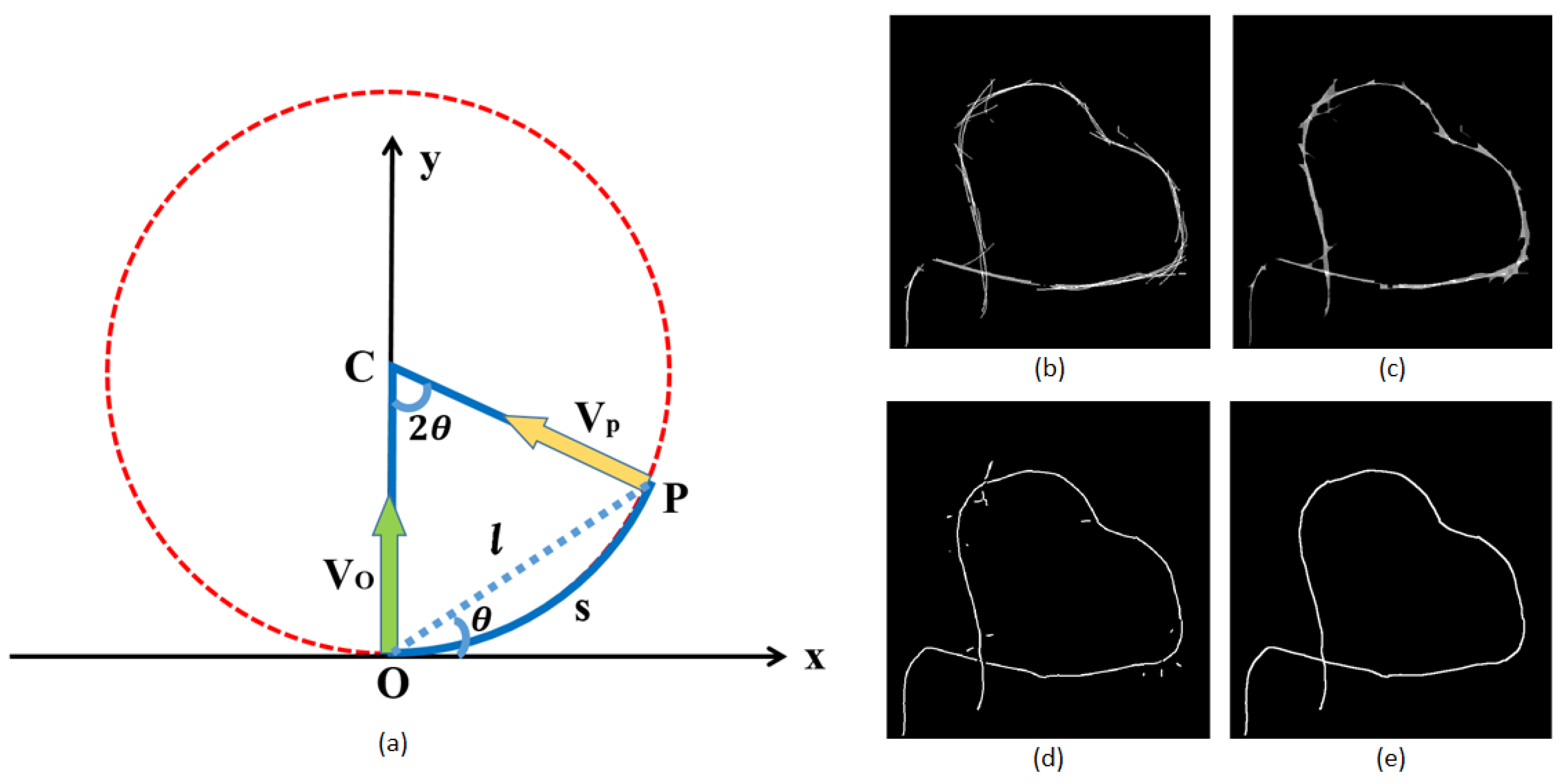
In the second stage of dense voting, the ball component of each tensor is discarded and the stick component is retained for voting with stick kernel. The diagram of stick voting is illustrated in Figure 6a. Suppose that $V_O$ and $V_P$ represent the normal vectors of voter O and receiver P, respectively. The most likely path from O to P is a circular arc with constant curvature. The saliency decay function of the stick voting can be written as follows:

$$DFs=e^{-\frac{s^2+c{k}^2}{{\sigma }^2}}$$

(21)

$$c=-\frac{-16ln\left(0.1\right)·(\sigma -1)}{{\pi }^2}$$

(22)

where s is the arc length between O and P; k is the curvature; and c controls the degree of curvature decay, which is related to $\sigma$. In this stage, voting is conducted from tokens to all locations in the neighborhood and the receivers accumulate the votes by tensor addition as well.

A new tensor field is created after tensor voting, and then, tensor analysis based on the saliency value is performed to classify all points into three types:

$$\left\{\begin{array}{cc}\mathrm{curve\; point},\hfill & \mathrm{if}({\lambda }_1-{\lambda }_2)>{\lambda }_2\hfill \\ \mathrm{junction\; point},\hfill & \mathrm{if}{\lambda }_1\approx {\lambda }_2>0\hfill \\ \mathrm{others},\hfill & \mathrm{if}{\lambda }_1\approx 0,{\lambda }_2\approx 0\hfill \end{array}\right.$$

(23)

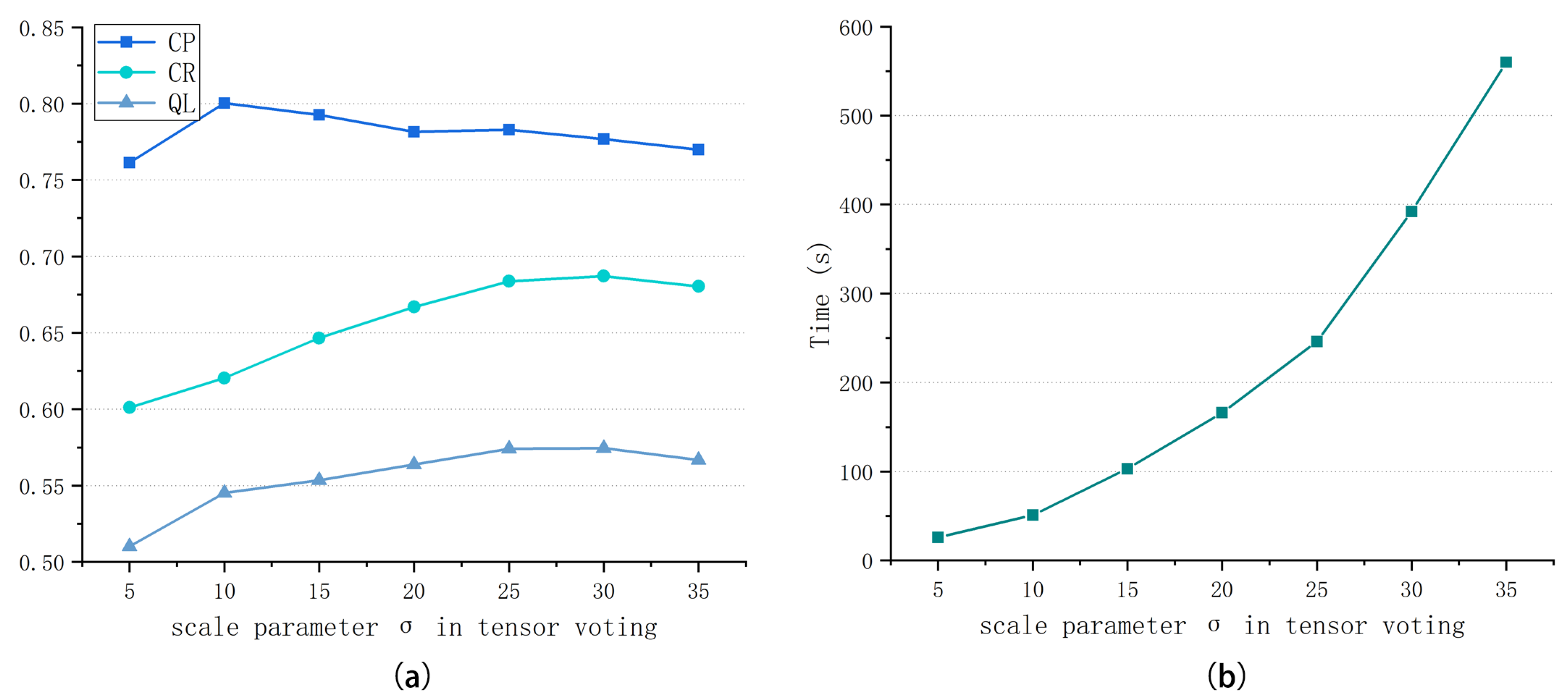
According to the classification criterions, we can obtain the stick saliency map, in which the road centerline tends to have local maximum values. Thus, Non-Maximum Suppression (NMS) is applied to extract the road centerline and to construct the road network. In the neighborhood, the non-maximum pixel is denoted as 0 and the maximum pixel is denoted as 1. As depicted in Figure 6d, the extraction result of TV-NMS consists of smooth curves. However, there still exists noisy fragments and discontinuities especially around junctions that need further refinement. The advantage of tensor voting is that the globally optimization is conducted automatically. As the only free parameter in tensor voting, $\sigma$ determines the range of data communication and will be discussed in the next section.

2.8. Spatial Regularization

Referring to previous works [8], a final spatial regularization algorithm is implemented based on perceptual grouping concepts. Regularization rules related to proximity and collinearity are used in this step aiming to eliminate undesired gaps and noisy line segments in the coarse road network. The rules have been completely described in [24,36]; thus, four criteria are briefly outlined as follows: (1) separate short centerlines are removed; (2) centerlines for which the endpoint distances are extremely short are merged; (3) centerlines which are collinear or nearly collinear are merged; and (4) when centerline $l_1$ intersects another extended centerline $l_2$ close to one of its ends, $l_2$ is lengthened to the intersection point. A continuous road network is generated after this basic and fast procedure. The final result is displayed in Figure 6e.

3. Experiments

In this section, parameters analysis and experimental results are performed to verify the effectiveness of the proposed method. Three popular criteria are used in quantitatively evaluation, including completeness (CP), correctness (CR), and quality (QL). The “buffer method” is adopted when comparing the extracted result and reference network. Concretely, CP is the percentage of reference network located in the buffer around the extracted network. CR is the percentage of the extracted network located in the buffer around the reference network. QL is a comprehensive index that combines completeness and correctness.

3.1. Dataset Description

The experiments are conducted on three high-resolution SAR images acquired by TerraSAR on HH polarization. Details of the test dataset are listed in

Table 1. Main information of the test dataset.

Study Site	Time	Location	Mode	Resolution	Size
0	20130414	Colorado Springs, American	HS	1.0 m	$600\times 576$
1	20130414	Colorado Springs, American	HS	1.0 m	$1940\times 1820$
2	20131022	Guam, American	ST	0.62 m	$1500\times 1748$
3	20160518	Guam, American	ST	0.36 m	$4416\times 4372$

. The resulting graph of each process in the previous sections is generated upon Study Site 0. Study Site 0 and Study Site 1 contain curved and intersecting road targets with the same width. Study Site 2 and Study Site 3 contain both straight lines and curves with different widths at about 8–20 m. Compared with Study Site 3, Study Site 2 includes more uniform dark areas such as buildings and parking lots, which may interfere with the road extraction task. Due to the diversity of road targets and relatively complex surroundings, a parameter analysis is carried out on Study Site 2. To obtain the ground truth, the reference road network is manually identified and labeled with the help of high-resolution Google Earth optical remote sensing images.

3.2. Parameter Analysis

The size of detection template is a key parameter in the directional road detector. As mentioned, template size directly affects the quality of the road response maps, the regularity of direction map, and time consumption. In order to highlight the road area, the length of template should be larger than the road pixel width, which is related to the image resolution and actual road width. Due to the multi-scale framework, we set the length of that template slightly larger than the pixel width of a medium road that is capable of producing satisfying extraction results. For quantitatively presenting the influence of template size on experimental results, CP, CR, and QL are plotted as functions of the length of detection template, as shown in Figure 7a. It can be seen that extraction results on Study Site 3 have overall low accuracy because of the disturbance from a complex background. CP increases with the growth of template size in general, whereas CP increases slowly when template size reaches a certain value. CR and QL first increase with the growth of the template size and then decrease when the template size becomes larger. On the one hand, a small template is seriously affected by speckle noise and incapable of extracting road area, resulting in low CP and CR. On the other hand, dark areas with low compactness are incorrectly identified as road targets when using a large template, leading to low CR. The time consumption of preliminary network generation on different template sizes is shown in Figure 7b, in which it is obvious that the larger template requires a longer computing time. Therefore, we choose a moderate template size, which can resist noise and extract road area correctly and completely. Empirically, the length parameter is approximately set as $10/resolution$. That is, Study Site 0 and Study Site 1 have a template length of 13, Study Site 2 has a template length of 17, and Study Site 3 has a template length of 27.

In regional quality evaluation, the evaluation function is a linear combination of four indicators, in which the weight parameters directly affect the performance of the evaluation function. The four indicators assess the quality of CCs from different aspects, which are all of practical significance for the road extraction task. Therefore, the change in each indicator should be reflected in the evaluation function, which requires similar ranges for the four indicators realized by adjusting the weight parameters. The values of the four indicators on all CCs at all scales are shown in Figure 8a. Figure 8c marks the statistical mean and standard deviation of each indicator, which roughly displays the range of indicators. It is obvious that the mean values of four indicators are quite different but we do not care. The standard deviation values of four indicators differ greatly as well. The value of LFI changes most drastically, while the value of DCI is the most stable. In order to balance the influence of each indicator in the evaluation function, we set the normalized reciprocal of the variance of each indicator as the weight of the corresponding indicator. In the experiment, we take ${\alpha }_L=0.2$, ${\alpha }_C=1$, ${\alpha }_S=0.3$, and ${\alpha }_D=0.25$. The values of the evaluation function on all CCs are shown in Figure 8b. CCs from low-level image layers are on the left, while CCs from high-level image layers are on the right. We can find that the value of evaluation function on CCs in low-level image layers is generally smaller than that in high-level image layers because high-level images mainly extract wide roads with prominent road features in which CCs have high reliability in being road segments.

Before road network refinement, CCs with high quality are selected through the threshold method based on the results of the quality evaluation. The threshold $T_E$ determines the quality of the extracted road network. If the value of $T_E$ is too large, few CCs will be reserved, resulting in discarding useful road segments and the reduction of continuity and completeness of the road network. If the value of $T_E$ is too small, more interfering regions will be retained and an unsatisfied road network will be produced. The influence of $T_E$ on experimental results is quantitatively analyzed in Figure 8d, in which CP, CR, and QL are plotted as a function of $T_E$. It can be seen that the value of CP increases slowly when $T_E$ is less than 0.63 and drops sharply when $T_E$ is greater than 0.63. CR overall increases with the growth of $T_E$ because of the strong probability of CCs with high possibility of being road segments. QL increases first and then decreases, reaching a peak around 0.7. Thus, $T_E$ is set as 0.7 in the experiment to obtain a satisfying result.

Tensor voting is used in road network refinement, in which scale parameter $\sigma$ is the only free parameter determining the scope of voting and calculation time. The purpose of tensor voting is to thin the preliminary road network after the morphological CLOSE operation and to remove undesired road gaps. Therefore, the value of $\sigma$ should not be too small to cover the range of the preliminary road network at each position and should ensure the continuity of network after non-maximum suppression. Meanwhile, the value of $\sigma$ should be larger than the half of road gaps to have the ability to eliminate the discontinuity of roads by perceiving the salience information in a tensor field. In addition, a large $\sigma$ increases the computation time notably, as shown in Figure 9b. To test the sensitivity of the proposed method to the variation in the scale parameter, CP, CR, and QL are plotted as functions of $\sigma$, as shown in Figure 9a. We can find that CP increases significantly when $\sigma$ is smaller than 10 and then decreases gradually with the increase in $\sigma$. CR and QL increase along with the growth in $\sigma$ and tend to be stable when $\sigma$ is larger than 25. On the one hand, road gaps are eliminated and a complete and correct network is generated with the increase in $\sigma$, leading to increases in CP and CR. However, a large $\sigma$ may result in “cross talk” heavily, which diverts the extraction result from the correct centerline position and especially takes place on road junctions, bringing about a decrease in CP. In conclusion, an appropriate scale parameter with medium value should be chosen to balance the detection performance and efficiency. Empirically, $\sigma$ is approximately set as $15/resolution$. That is, $\sigma =15$ in site 0 and site 1, $\sigma =25$ in site 2, and $\sigma =30$ in site 3.

3.3. Experimental Results

The experimental results on three study sites are displayed in Figure 10, and the quantitative indexes are recorded in

Table 2. Quantitative comparison with different methods on three study sites.

Method	Study Site 1			Study Site 2			Study Site 3
	CP	CR	QL	CP	CR	QL	CP	CR	QL
Comparison 1	0.7497	0.7325	0.5881	0.6686	0.4761	0.3852	0.8605	0.7455	0.6630
Comparison 2	0.8473	0.8179	0.7132	0.7780	0.5698	0.4891	0.9340	0.7668	0.7266
Comparison 3	0.7953	0.8648	0.7063	0.6707	0.6244	0.4757	0.9337	0.7628	0.7148
Proposed	0.8670	0.8920	0.7836	0.7830	0.6837	0.5741	0.9296	0.8649	0.8173

. The simple road structure and clean background lead to a high-quality extraction result on Study Site 1, in which only a few roads with weak features are ignored. The values of CR and QL are lower than 0.7 on Study Site 2, resulting from the false recognition of objects that have similar appearances to road targets. Some dark building regions are identified as road area. Meanwhile, some straight roads are deformed to curves due to the thinning method of 3-order polynomial curve fitting, which is unsatisfying and needs further improvement. The very high resolution of Study Site 3 benefits the road network extraction task; thus, we acquired promising results with high values of CP, CR, and QL. Nonetheless, there are still narrow roads that have not been reconstructed in a network because the indistinct features are submerged in complex building surroundings. Simultaneously, long shadows are incorrectly extracted as road targets. In general, most roads have been successfully extracted and the generated networks are relatively continuous and intact based on our method. The quantitative evaluation results are also acceptable and are mostly larger than 0.75.

4. Discussion

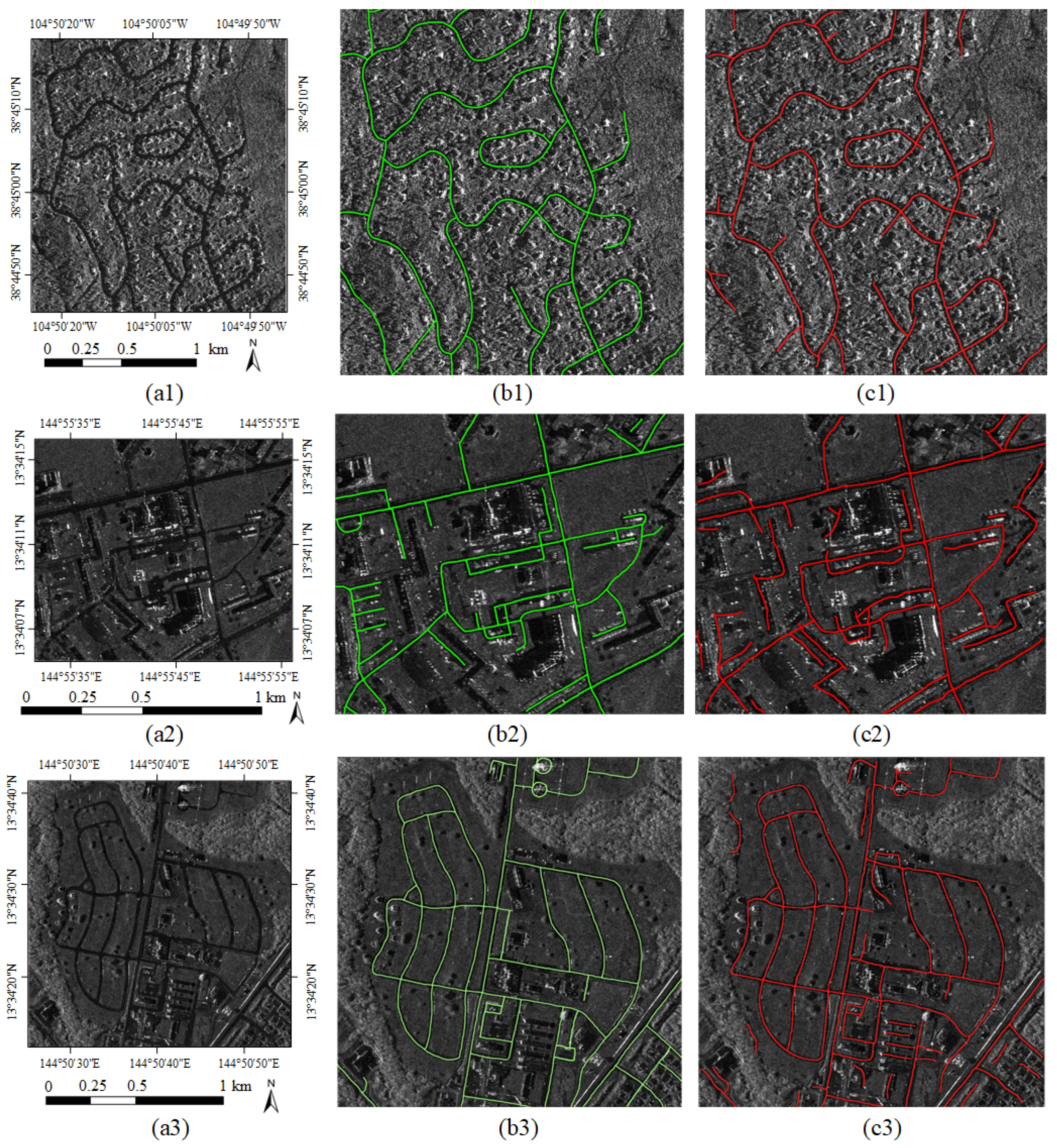
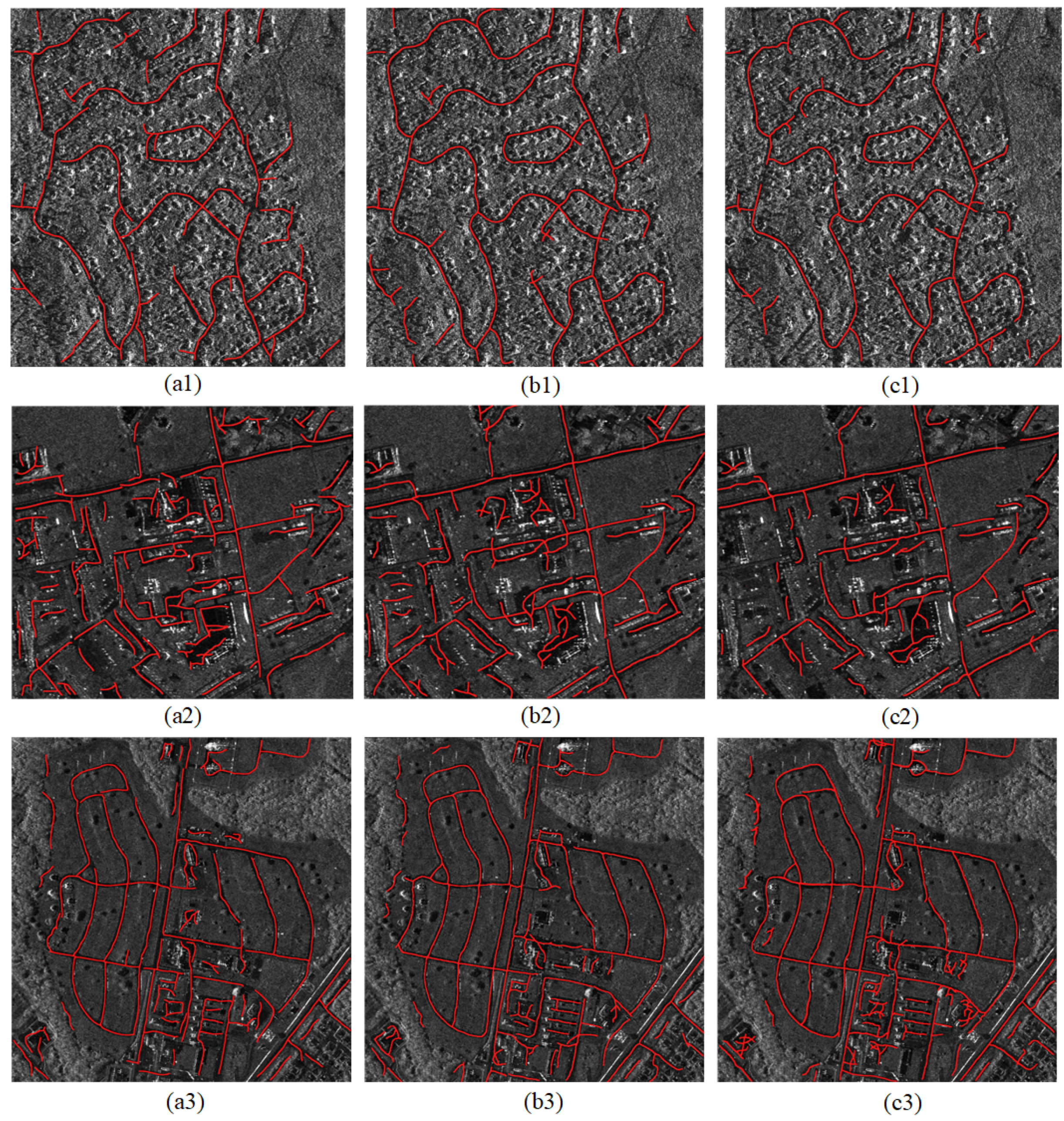
In this section, related experiments are conducted to comparatively demonstrate the effectiveness of the proposed method, as shown in Figure 11. The numerical evaluation is reported in Table 2. It is worth mentioning that parameters in related experiments are adjusted to gain best networks for fair comparison.

To test the practicality of the multiscale framework in the road network extraction task, a similar algorithm conducted on a single scale (original scale) is implemented, denoted as Comparison 1. As the template size of directional road detector is fixed in this paper, the multiscale framework plays an important role in extracting road targets with different widths; thus, a D1D2 operator [6] with diverse template orientations and sizes is used as the road detector in the single-scale contrast experiment. Beyond that, we use the same thinning and refinement method to obtain extracted results. As shown in Figure 11a, the completeness and continuity of road networks obtained by Comparison 1 are inferior to that extracted by our method for more gaps. Furthermore, the values of CP, CR, and QL distinctly decline in Comparison 1. In the image pyramid, high-level images can reflect the overall trend of the road network and tend to extract wider main roads. In contrast, low-level images are rich in details and used to extract narrower paths. The employment of the multiscale framework combines the extraction results of different levels; hence, a relatively complete network can be obtained. Although the multi-direction and multi-size D1D2 operator adopted in Comparison 1 likewise has the ability to detect road targets with different widths, its fault tolerance rate is not up to the proposed method. The quality of extracted network is closely related to the quality of CCs in directional decomposed image layers. However, the CCs in Comparison 1 are determined by the once generated direction map, which is less reliable due to the randomness of local information. Considering both scattering CCs from well-detailed low-level images and regular CCs from trend-salient high-level images, the proposed method integrates the multiscale information based on weighted summation and tensor voting to produce promising results.

To prove the availability of regional quality evaluation, an identical algorithm without quality evaluation on CCs is implemented, denoted as Comparison 2, in which only CCs with small pixel area are removed as described in [32]. We can find from Figure 11b that, compared with networks generated from our method, the networks without regional quality evaluation are less regular and contain more redundant curves, especially in the uniform dark areas. As noted in Table 2, the lack of quality evaluation on CCs has a little effect on CP but a large effect on CR. The evaluation function is regarded as the probability that the current CC is located in a road area. On the one hand, the regional assessment can further screen out the road area through the threshold method. On the other hand, different weights are given to CCs according to different credibilities. Due to the sole use of the pixel area as the criterion to select valuable regions, many CCs located in non-road area are retained, resulting in a redundant extracted network with low correctness. Meanwhile, there is no distinction between high-quality and low-quality road segments. During road network optimization, road curves with low quality tend to deviate the network from the correct road centerline, leading to irregular results.

Comparison 3 refers to a recently proposed method [32] that develops the idea of direction feature grouping. In this paper, we introduce an improved algorithm on the basis of directional decomposition; thus, Comparison 3 is implemented to verify the effectiveness of our method. A support vector machine is used to classify road and non-road regions in [32]; therefore, the value of CR tends to be high in Comparison 3. In our method, rational quality evaluation achieves a similar purpose. With the constructed multiscale framework, our method obviously balances the completeness and correctness, performing better than Comparison 3 visually and numerically.

The effectiveness of the proposed method has been analyzed and validated comparatively. Although the general structure of road targets has been almost completely extracted, the method still has some drawbacks. Objects that have similar appearance to road targets in SAR images cannot be distinguished, such as rivers and long buildings. As the only input in our method, intensity information hardly provides sufficient features for accurate road detection. Moreover, straight roads are likely to be smooth curves in the extracted results because of the polynomial curve fitting thinning method. The performance of the proposed method depends on the parameter setting, which requires parameter adjustments in special scenarios.

For road network optimization, TV-NMS plays an important role in automatically learning the correct road position from repetitious road curves. In most cases, road targets can be accurately located through TV-NMS. However, output networks may deviate from the road centerlines when crisscross roads densely distribute and seriously interfere with each other. Meanwhile, the missing parts always occur around road intersections, which needs further processing such as spatial regularization. In our method, the input of tensor voting merely contains sparse pixels with location and amplitude information, whereas direction information is also capable of guiding the voting operation. We believe that it is a worthy attempt to directly input road pixels with credible direction information to tensor voting.

5. Conclusions

In this paper, we propose an improved method for road network extraction from high-resolution SAR images, which is capable of capturing road targets with different widths and appropriate for both straight and curved road targets. The major contributions of our method include the multiscale extraction framework and regional quality evaluation. Specifically, image pyramid along with a fixed-size filter is constructed to implement multiscale analysis, in which a directional road detector is designed to highlight the potential road area. After directional decomposition based on the binary segmented map, regional quality evaluation is conducted to quantitatively access the probability of segments being located in a road area. Road network is generated by the weighted sum of polynomial curves and optimized via tensor voting and spatial regularization. Experimental results and comparisons on TerraSAR images prove the effectiveness of our method. The developed multiscale framework has a higher fault tolerance for road network extraction and achieves an improvement in quality measures by about 18% compared to the D1D2 detector. As a region-based secondary identification for road targets, regional quality evaluation significantly promotes the correctness of extracted road networks by about 10%. Future works can be carried on the following aspects: (1) integrating multi-source images to achieve road information fusion, (2) applying deep learning to automatically extract deep features and segment road areas correctly, and (3) conducting straight line detection to preserve the straightness of some road lines.