Abstract
Photogrammetric models have become a standard tool for the study of surfaces, structures and natural elements. As an alternative to Light Detection and Ranging (LiDAR), photogrammetry allows 3D point clouds to be obtained at a much lower cost. This paper presents an enhanced workflow for image-based 3D reconstruction of high-resolution models designed to work with fixed time-lapse camera systems, based on multi-epoch multi-images (MEMI) to exploit redundancy. This workflow is part of a fully automatic working setup that includes all steps: from capturing the images to obtaining clusters from change detection. The workflow is capable of obtaining photogrammetric models with a higher quality than the classic Structure from Motion (SfM) time-lapse photogrammetry workflow. The MEMI workflow reduced the error up to a factor of 2 when compared to the previous approach, allowing for M3C2 standard deviation of 1.5 cm. In terms of absolute accuracy, using LiDAR data as a reference, our proposed method is 20% more accurate than models obtained with the classic workflow. The automation of the method as well as the improvement of the quality of the 3D reconstructed models enables accurate 4D photogrammetric analysis in near-real time.
1. Introduction
Structure from Motion (SfM) photogrammetry is a technique used to reconstruct 3D models from unregistered, overlapping image sets. This approach is a low-cost and flexible surveying tool that can be considered as an alternative to techniques such as Light Detection and Ranging (LiDAR) that usually require high-cost equipment.
Due to advances in the processing techniques of digital photogrammetry and computer vision, results comparable to LiDAR can be achieved under specific circumstances, i.e., capturing 3D data with great precision and high quality [1]. The large number of publications in the last five years using point clouds calculated with image-based 3D reconstruction to analyse and monitor objects and surfaces, for example building structures [2,3,4,5] or natural surfaces [6,7,8,9,10], confirm the popularisation of the use of this technique [11].
1.1. Basic Prinicples of SfM Photogrammetric Systems
Basic principles of SfM photogrammetry are widely described in previous publications such as [9,10,12,13]. The principal idea relies on estimating point positions in 3D (object space) from corresponding points on 2D surfaces (image space). The workflow can be performed in different software, both commercial and open source [8]. Some of these suites, such as Agisoft Metashape, allow for automation of the processing chain using scripts via API. Hence, the usual pre-processing steps used to reconstruct 3D models such as image masking, marker detection or filtering of outlier points can be automated.
Capturing the overlapping images to calculate 3D models can be considered from two data acquisition perspectives, either using a set of stationary cameras pointing at the object of interest or using a single camera moving around the object of interest, i.e., fixed and mobile systems, respectively. Fixed systems compute the 3D model with images always taken from the same position with a unique camera for each. Therefore, the photogrammetric processing is based on limited camera perspectives. This has consequences for the reliability of the image-based 3D reconstruction. Micheletti et al. [14] demonstrated that by providing an adequate spatial distribution of the image network geometry, acceptable accuracies can be achieved even using small image sets. However, they considered one camera for all images, which is not the case for stationary setups. In contrast to capturing the images with a single camera, where only one set of interior parameters have to be estimated (i.e., principle length, principle point, and distortion parameters), each new camera entails considering additional interior camera parameters because the physical properties are different for each camera [15]. Considering these challenges of fixed systems, Kromer et al. [16] were able to achieve detection limits between 2-3 cm, in the ranges required for monitoring prefailure deformation on slopes with only five stationary cameras.
Besides the geometric considerations of the imaging network, using fixed systems entails further difficulties regarding the operation of these systems in an autonomous manner. In this regard, a communication network has to be provided to transmit the data or to check the system status. Furthermore, a sufficient energy supply is required. Despite these constraints, fixed camera stations for SfM photogrammetry are growing in the field of geoscience monitoring and the last year has seen publications on a fixed rockfall monitoring system developed with low-cost cameras published by Blanch et al. [13], an array of cameras used to study rock slope hazards on a road published by Kromer et al. [16] and an autonomous terrestrial stereo-pair photogrammetric monitoring system developed to observe rockfalls in mining environments published by Giacomini et al. [17].
Mobile systems such as UAVs bring greater flexibility. Large sets of photographs can be acquired from a single camera, allowing for a larger number of observations from several perspectives for the bundle block adjustment. This increase in input data allows for more reliable photogrammetric models. Verma and Bourke [18], for example, used more than 50 photographs at close range (<2 m) to obtain sub-millimetre-resolution models of rock faces using calibrated error evaluation chart. In addition, the ability to extend the mobile system by mounting a camera onto an Unmanned Aerial Vehicle (UAV) allows areas and perspectives to be reached that are difficult to reach on foot [19]. Commercial ready-to-fly solutions have led to an increase in the use of aerial photogrammetry in recent years [8,20,21,22,23,24]. On the contrary, the inability to take pictures both from the same exact position (as in a fixed system) and at a high temporal frequency makes it difficult to use algorithms and workflows based on the redundant use of image bursts created to obtain higher quality models [13] as we will see in this paper, although experience with multi-epoch imagery workflows such as [1,25] demonstrates a certain capacity for improvement with mobile systems.
SfM photogrammetry is considered a low-cost approach compared to other methods of terrain observation [9]. However, the cost of photogrammetric systems varies widely depending on their configuration. Mid to High-cost systems (>1.000 EUR) are composed of commercial solutions using cameras and devices with large sensors of high resolution. These cameras, usually DSLR or mirrorless full frame cameras (43 mm sensor diagonal), can obtain images of more than 24 mega pixels. They have high sensitivity photoreceptors, produce very little digital noise and hence possess exceptional image quality with a high capacity to extract information from dark and bright areas due to the high dynamic range of these images. Furthermore, these cameras can use high-quality fixed lenses that enable the capture of images with very little distortion and great sharpness, which is advantageous for obtaining high quality models [8]. There have been several studies implementing photogrammetric systems with commercial, high-quality cameras [16,26,27,28]. However, one limitation of these kinds of devices in fixed camera systems is their cost and the large amount of data that needs to be transferred remotely, as the size of each image can reach more than 30 MB.
Other than that, low-cost photogrammetric solutions involve the use of very simple photographic systems (less than a hundred euros). These systems are based on uncoupled camera modules controlled by single-board computers, such as Raspberry Pi [29], or microcontrollers, such as Arduino (open-source) systems. These cameras are associated with photographic sensor diagonals of less than 16 mm with resolutions that vary between 5 and 12 mega pixels. To reduce costs, they are equipped with low-quality plastic lenses that usually result in strong distortions. The quality of the images obtained with these cameras, revealing low sharpness and high digital noise, are the main constraint for their application in 3D measurement tasks [13]. However, low-cost solutions are easy to implement and simple to program. In addition, these systems are ideal for installation at sites exposed to destructive phenomena such as flash floods or mass movements. Various examples of low-cost photogrammetry implementations can be found in the field of geosciences [13,30,31,32].
1.2. Improvements of SfM Photogrammetric Workflows
Strategies to obtain improved SfM photogrammetric models are required, especially in scenarios that entail the use of fixed and low-cost camera systems. These improvements can be implemented at different stages of the SfM photogrammetric workflow. Regarding the data collection stage, studies have been carried out to investigate the impact of using High Dynamic Range (HDR) images instead of conventional photographs to reconstruct 3D models in the fields of cultural heritage documentation [33] and geomorphic change detection [34]. Other studies have examined the use of high-resolution photographs (gigapixel) [35,36]. Furthermore, attempts have been made to enhance SfM photogrammetric models by stacking images in order to reduce the noise from digital cameras [31], although with inconclusive results.
Several studies have focused on improving the SfM photogrammetric results by pre-processing of the input data, such as enhancing the image quality [37] as well as pre-defining calibration parameters and adjusting the imaging network configuration. For instance, James and Robson [38] mitigated systematic errors common for UAV models [8] by obtaining additional convergent images to enhance the strength of the image network geometry [39]. Furthermore, it is important to retrieve suitable lens calibration parameters [39], which is especially the case for consumer grade cameras that usually exhibit stronger distortions. More recently, Elias et al. [40] carried out a study to estimate the effect of temperature changes on low-cost camera sensors, highlighting the importance of also considering the temporal stability of cameras, especially during long-term observations.
Another focus has been on improvement of the SfM workflow itself to obtain 3D models with the highest possible quality, allowing for multi-epoch imagery change detection. The differences between these methods depend both on the characteristics of the object to be studied and on the possibility of automating processes and locating ground control points. Verna and Bourke [18] presented a method that is capable of obtaining sub-millimetre accurate small-scale digital elevation models at close range. Another setup developed by Kromer et al. [16] enabled the detection of rockfalls automatically from time-lapse imagery. Eltner et al. [41] introduced a time-lapse SfM photogrammetry workflow that enabled the almost continuous detection of soil surface changes with millimetre accuracy. The methodology proposed by Feurer and Vinater [25] improves SfM photogrammetry-derived 3D models by joining imagery from different points in time during image matching and 3D reconstruction. This has the advantage that systematic errors might be spatially consistent over time and therefore negligible during change detection. This methodology was put into practice by Cook and Dietze [1].
Finally, methodological proposals have been made to improve the results, regardless of the pre-processing and workflow used. For instance, the PCStacking (i.e., point cloud stacking) algorithm developed by Blanch et al. [13] improves the 3D models using subsequent photogrammetric reconstruction solutions for images shot over a short time interval. Another recently developed strategy to enable more reliable change detection involves the introduction of precision maps by James et al. [42]. Together with the M3C2 tool from Lague et al. [43], the strategy allows change detection results to be obtained with information about the significance of the measured change.
The research presented in this paper proposes a new automatic pipeline to obtain improved 3D models using fixed time-lapse cameras. The methodology is based on a fully automatic workflow of the whole data acquisition and processing routine, from capturing images remotely with various cameras to performing change detection. This study proposes a new method that allows the calculation of photogrammetric models with high spatial frequency, high temporal resolution and high accuracy, therefore achieving higher quality in automatic change detection.
2. Materials and Methods
2.1. Pilot Study Area
The system was developed on the Puigcercós cliff (Catalonia, NE Spain) (Figure 1a), which is part of the Orígens UNESCO Global Geopark. The rock face (123 m long and 27 m high) is the result of a large rototranslational landslide [44] that occurred at the end of the 19th century [45,46]. The structure of the zone (Figure 1b), its high rockfall activity and low risk (due to lack of exposed elements) have made it an ideal area to develop methodologies such as the detection and spatial prediction of rockfalls by means of Terrestrial Laser Scanner (TLS) [47], the clustering approach workflow for rockfall detection [48], the spatio-temporal analysis of rockfalls pre-failure deformation [49,50] and the enhanced workflow PCStacking described by Blanch et al. [13]. In addition to studies related to rockfall monitoring, the site is an ideal natural laboratory for developing new observational techniques in the field of geosciences [51] such as the estimation of mass movements based on seismic observation [52] and the use of GPS data to study the fractures and slope stability [53].
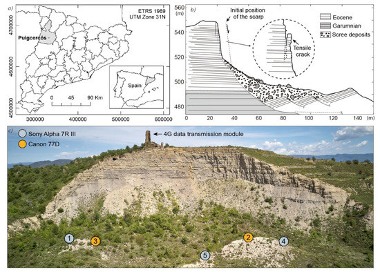
Figure 1.
(a) Puigcercós location in Pallars Jussà region, Catalonia, NE Spain. (b) Geomorphological scheme of the Puigcercós cliff and main rockfall mechanism (modified from Royán et al. [49]). (c) Distribution of the camera modules in front of the Puigcercós cliff.
2.2. Equipment
Images for the image-based reconstruction of high-resolution point clouds were taken by a photogrammetric system developed ad hoc for the Puigcercós pilot study area. The system consists of five camera modules, a data transmission module (Figure 2) and a workstation. Images were taken by the camera modules fixed at five locations in close proximity to each other (Figure 1c) on small elevations on one of the transverse ridges created by the ancient landslide. The average distance between the camera modules is 30 m and the distance to the main rock face of the cliff is around 100 m. The maximum distance between the transmission module and the camera modules is about 130 m. Each camera module consists of a high-performance commercial camera with a fixed lens, a microcomputer with RTC (Real Time Clock), an external WiFi antenna, a battery and a solar panel. These modules were mounted in dustproof and waterproof metal enclosures (Figure 2).
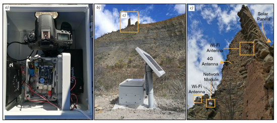
Figure 2.
Components of the photogrammetric system mounted at Puigcercós. (a) Internal view of the camera module composed of a Canon 77D camera and the auxiliary control system. (b) External view of a camera module in front of the Puigcercós cliff. (c) Installation site of the 4G data transmission module on the upper part of the rock cliff. The two sectorial Wi-Fi antennas, the router module and the battery can be seen in the tower.
Three of the five modules use a full-frame (35.9 × 24 mm) mirrorless Sony Alpha 7R III with a resolution of 42.4 MPx (pixel pitch of 4.51 µm). These cameras are equipped with a 35 mm f/2.8 lens. The other two systems use a DSLR camera Canon 77D with a cropped sensor APS-C (22.3 × 14.9 mm) and with a resolution of 24.2 MPx (pixel pitch of 3.72 µm). The Canon cameras are equipped with a pancake 24 mm f/2.8 lens. The use of a 24 mm lens on an APS-C cropped sensor generates the same field of view as using a 35 mm full frame lens. Sony and Canon modules are alternatively positioned in the study area (Figure 1c). The theoretical depth error for this camera setup, assuming a stereo-classic case and error free camera parameter estimations, amounts to 2.3 cm [9]. However, higher accuracies can be expected because five instead of two cameras capture the same area of interest with slightly convergent perspectives.
The microcomputer used is a Raspberry Pi 3 Model B+ [29] from Raspberry Pi Foundation. It is in charge of scheduling data acquisition, capturing the images, transmitting the data and managing the battery of the devices. A commercial board Witty Pi 2 from UUGear is used as a real-time clock and power management system for Raspberry Pi 3, and to manage voltage differences and schedule the system. Finally, a solar panel (20 W) and an AGM battery (7000 mAh) make each module autonomous in terms of power (Figure 1b).
A 4G transmission module is based on a 50 dB 4G unidirectional antenna, a Teltonika RUT950 router and two 10 dB WIFI sectorial antennas (Figure 1c) that project the network from the top of the cliff to the area where the camera modules are installed (see Section 2.2). Again, a solar panel and an AGM battery supply power to these devices.
The last part of the photogrammetric system is the workstation/server. This computer is in charge of performing server functions by receiving and storing the images. Furthermore, the workstation performs the entire workflow fully automatically to eventually obtain the high-resolution photogrammetric models and their change detection map. The workstation in this study consisted of commercial components of a medium–high range with an Intel(R) Core(TM) i9-7900X processor of up to 4.30 GHz, with 64 GB of RAM and a NVIDIA GeForce GTX 1080 Ti graphics card.
2.3. Data Acquisition
Images were obtained at a sub-daily frequency for 4D analysis of the rockfalls. The camera modules captured four images in a burst mode three times per day. Thus, three times four images were taken from five camera modules, resulting in 60 images of the Puigcercós cliff every 24 hours. The images were taken at 9 a.m., 1 p.m. and 6 p.m., although the most-used images were taken at 6 p.m. to avoid shadows on the escarpment. All images are obtained in JPG format using the highest possible quality. The focus point is set manually, and the exposure time is automatically calculated according to the aperture, set at f/11 to obtain an acceptable depth of field. The configuration of the photogrammetric system can be easily modified to increase the acquisition of images on a more exhaustive daily basis. The scripts of the photogrammetric system that allow for scheduling, capturing and sending the images remotely to the server were developed using the open-source Python programming language (version 3.7) [54]. The images were transmitted daily to the workstation where, after server storage, the automatic photogrammetric processing of the images was activated to obtain the 3D models to carry out change detection, also automatically.
LiDAR data was acquired as the reference dataset. The data was obtained with the ILRIS-3D-Optech TLS (Terrestrial Laser Scanner). This high precision device allows the generation of a point cloud (2.500 points/s) with the 3-D coordinates (X, Y, Z) of each point with an accuracy of 7 mm when scanning at a distance of 100 m, according to the manufacturer’s specifications. The standard deviation of the instrumental and methodological error was defined as 1.68 cm at an average distance of 150 m by Abellan et al. [47] and derived from this parameter, the change detection threshold for the scanning distance of the Puigcercós cliff was defined as 3.0 cm by Royan et al. [49] The TLS data was captured in October 2019.
2.4. From 2D to 4D–Workflow for Automatic Change Detection with Time-Lapse Imagery
To highlight the improvements made in this study, the methodology is divided into three sections: (1) Workflow part I, which refers to the tools developed for automatic pre-processing of data; (2) Workflow part II, which focuses on the improved photogrammetric workflow to acquire time-lapse 3D data, called multi-epoch multi-imagery (MEMI); and (3) Workflow part III, which introduces an automated change detection approach demonstrated at Puigcercós (Figure 3). These three steps are part of a whole working pipeline that allows change detection models to be obtained automatically from the different images, as described be-low.
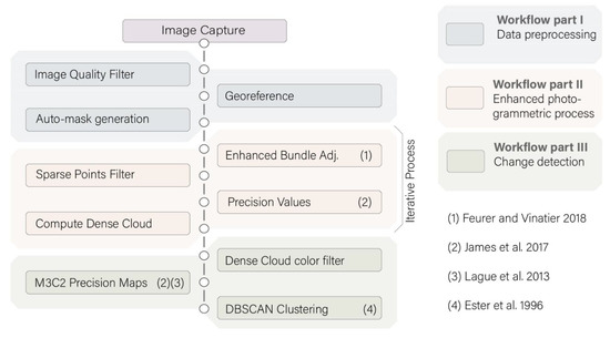
Figure 3.
4D pipeline designed for the automatic analysis of rockfalls in Puigcercós. The colours represent different parts of the process grouped according to their description in the manuscript.
2.4.1. Data Pre-Processing (Workflow Part I)
Data pre-processing is essential because images were not captured under controlled environmental conditions. Image quality and data acquisition geometry change due to lack of maintenance, excess humidity, presence of fog, changing lighting conditions, vegetation growth, temperature changes and small variations in camera positions because of impacts, animals or metal dilations during the long-term observation period. Data pre-processing is particularly important because the success of the following stages strongly depends on the quality of the input data.
Several tools have been developed to perform data editing steps that users usually need to do when preparing data for photogrammetric processing. These steps utilize techniques from computer vision and image analysis to enable geometric georeferenced models of maximum quality. The developed tools comprise:
- (a)
- Image Quality Filter. The cliff is located in a mountainous area where fog, snow and heavy rainfall are frequent, making the use of quality filters mandatory. Images are filtered based on an image quality estimation made with the Open CV library [55]. The applied function is a Laplacian variation [56,57]. If images are not sharp enough due to unfavourable environmental conditions, the time-lapse photogrammetry processing workflow is stopped at this step.
- (b)
- Georeference. This tool allows one to determine if the cameras have changed their position, based on a reference image [58]. Although the camera systems are fixed to the ground, camera movements are possible, e.g., due to temperature changes, wind or animals. Also, changes in the interior camera geometry are likely due to heating and cooling of the housing [40,59]. In this study we used the Lucas–Kanade method [60,61], also implemented in OpenCV, which has been shown to be suitable for tracking targets in geoscience applications [62]. It is used to track control points, assigned in a reference image, in the target image. To ensure good georeferencing Ground Control Points (GCPs) are located in the images, thus providing their 2D coordinates, their corresponding 3D coordinates are assigned in object space. In this study, the real-world coordinates of GCPs were extracted from a TLS point cloud of the escarpment and were assigned manually by correlating TLS points with image pixels. The precision of this approach of GCP retrieval is discussed in Section 4.3.
- (c)
- Auto-mask generation. During the image-based 3D reconstruction steps a mask was applied to calculate a dense, high-resolution, large data volume point cloud only for the area of interest. Thus, the images are masked to the area of interest in their field of view. Due to changes in the camera geometry these masks need to be updated. The tracked GCPs allow calculation of the parameters of a perspective transformation to warp the binary masks from the reference images to the targeted images according to their movements.
2.4.2. Enhanced Photogrammetric Process (Workflow Part II)
The second part of the presented workflow is an advancement of the photogrammetric workflow described in Feurer and Vinatier [25] and Cook and Dietze [1]. In these studies, it was referred to as the time-SIFT or multi-epoch imagery workflow. We will use the acronym MESI (Multi-Epoch Single-Imagery) to refer to this workflow. Furthermore, an enhanced workflow was introduced that exploits the redundancy of images due to bursts of captured images from the fixed time-lapse camera setup for the multi-temporal analysis (Figure 4), and this is referred to as Multi-Epoch Multi-Imagery (MEMI).
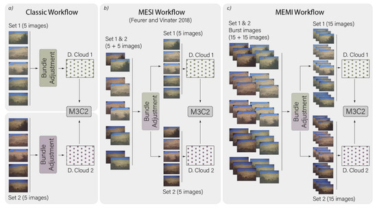
Figure 4.
Three different SfM photogrammetry workflows to calculate multi-temporal point clouds for change detection. The colour shading denotes images obtained at different time epochs. (a) The classic workflow corresponds to the standard SfM photogrammetric approach. (b) The multi-epoch imagery workflow (MESI) adopts the method defined by Feurer and Vinatier [25], i.e., joining images from multi-epochs during image matching and bundle adjustment. (c) The Multi-Epoch Multi-Imagery (MEMI) workflow considers (additionally to b) redundant image bursts from each epoch.
In the classic time-lapse SfM photogrammetry workflow two separate bundle adjustments are performed to reconstruct the image geometry and the sparse point cloud, which refers to the 3D coordinates of the tie points [41]. Each bundle adjustment is done with the individual photos of the single epochs, i.e., individually for set 1 and set 2 (Figure 4a). In each set there is only one image from each camera. Eventually, the dense point clouds are obtained after each bundle adjustment. These point clouds are geo-referenced in a local, scaled coordinate system via GCPs extracted from the LiDAR scan. However, due to errors, e.g., during their tracking in the images, alignment errors between the point clouds are possible, which is partly compensated for by ICP-type (Iterative Closest Point) algorithms [63].
For the MESI workflow the method described in Feurer and Vinatier [25] and Cook and Dietze [1] is implemented, performing image matching using data from different time epochs. The time-SIFT approach is described as “joining multi-epoch images in a single block” [25]. The result of the bundle adjustment using MESI is a sparse point cloud that contains tie points matched across overlapping frames from different points in time (Figure 4b). Only one bundle adjustment is performed to calculate sparse 3D point clouds, merging image Set 1 and Set 2. Consequently, spatially correlated systematic errors typical for SfM photogrammetry [42] are assumed to display similar magnitudes across the epochs and therefore are mitigated during change detection after differencing of point clouds. The bundle adjustment with merged multi-epoch single images also has the advantage that the observation number increases strongly (several thousand more image points) while only a few additional unknowns (14 for each camera, i.e., exterior and interior camera orientation parameters) are introduced, increasing the reliability of the estimated parameters. After estimating the camera parameters, the images are separated again into the original sets to calculate the two dense point clouds using only images from the same epoch. The computed dense models do not require further alignment because they were already aligned in the same coordinate system during the bundle adjustment, considering the across-epoch tie points.
Besides the multi-epoch merging of images during 3D reconstruction, the improvements due to capturing bursts of photographs during one point in time shown in Blanch et al. [13] were also implemented in this study. Thus, image bursts from each epoch and multi epoch imagery were combined. The dense point clouds were computed in the automatic multi-epoch multi-imagery (MEMI) workflow using more than one image per camera location (Figure 4c). Therefore, each dense point cloud was created using 15 images (per epoch) instead of five as in the classic and MESI workflow. This resulted in two dense point clouds, but for the MEMI approach each one was calculated with the burst of images taken during different epochs. Again, the clouds share the geo-reference and spatially correlated errors (calculated from all 30 images in the bundle adjustment). This enables good alignment to enhance the detection of changes between models. However, this approach only works if stable areas are large enough within the field of view of the cameras. This workflow was implemented using Agisoft Metashape Pro (version 1.6.6) [64] software and was automated using the available Python API (version 1.6.4) [65]. In line with previous work [16], a further processing step was integrated into the automatic workflow. To improve the accuracy of the 3D reconstruction a filter, based on a reprojection error and reconstruction uncertainty, was applied to the sparse point cloud after the bundle adjustment (Figure 3) to reduce outliers.
The last step of the automatic photogrammetric process involved a workflow introduced by James et al. [42] (Figure 3) to export sparse point coordinate precision estimates from Metashape [42]. Given the sensitivity of the precision parameters an iterative bundle adjustment was performed until the precision values of the control points and the tie points stabilized. The sparse point precision was used to calculate 3-D precision maps [42]. These precision maps improve the level of detection (LoD) estimation because instead of considering a uniform value for the entire point cloud, a LoD is calculated considering the spatially correlated errors from the 3D reconstruction [42].
2.4.3. Change Detection (Workflow Part III)
The final step of the introduced 4D pipeline, after reconstructing multi-temporal 3D models of high quality, is automatic change detection. First, a colour filter was applied to the dense point cloud to remove shadowed areas because in this study the shaded areas were not correctly calculated and therefore led to errors in the detection of changes [65].
Afterwards, the M3C2 algorithm [43], integrated into the software CloudCompare (version 2.11) [66], was used to calculate the model differences between different epochs considering the precision maps option [42]. The point cloud difference calculation resulted in a new point cloud with an additional scalar containing the metric distances between the compared dense clouds. Thereby, the DBSCAN algorithm [67] was used to automatically extract clusters of points that had difference values above a threshold and a minimum number of neighbours within a certain distance. The use of this methodology for LiDAR point clouds is explained in detail in Tonini and Abellan [48]. As a result of the application of the clustering algorithm, a new point cloud was generated that only contained points that match the characteristics required to be part of a change cluster.
The introduced automated enhanced workflow for change detection from photogrammetric models ends at this point. The provision of the source-code enables the workflow to be implemented and adapted according to the individual applications and their specific analytical requirements.
Due to automation, the 4D pipeline presented in this study obtains multi-temporal 3D point clouds from the automatically captured input data with all the changes identified ready for further analysis.
2.5. Performance Assessment
To assess the performance of the three different approaches, the classic approach, MESI and MEMI were compared for a period when no changes occurred. Three tests were designed to assess the relative accuracy of change detection, to evaluate the interior point cloud precision and to determine the absolute point cloud accuracies by comparing the point clouds to each other and to an independent LiDAR reference.
2.5.1. Relative Accuracy of Detected Changes
The three workflows described in Figure 4 were performed with the same input data to observe potential differences between the resulting change detection models, and to assess the accuracy of change detection, without considering absolute errors of change. To enable the evaluation of absolute accuracies of change detection independent TLS measurements from the same time period would be needed [1].
In order to analyse the relative accuracy, two different tests were performed. The input data for each test consists of a burst of images captured by each of the five camera modules on two consecutive days. Due to the use of images from contiguous dates, with no obvious changes in the area of interest, it is possible to assess the performance of the multi-temporal change detection because no changes should be visible in the final change map. For the first test, the images considered were taken on 8 and 13 November 2019. Due to the setup configuration at that time, bursts of three images were captured by each of the five camera modules. The second test was performed using images captured on the 23rd and 24th of May 2020. As a result of a system improvement, the second test benefitted from a higher burst, with four images captured by each of the five camera modules.
To assess in more detail the improvement in change detection due to the increased number of images from each burst, an additional evaluation was performed, using the MEMI workflow, but with a burst of two images instead of a burst of four. The MEMI workflow using only two images is referred to as the mild MEMI workflow (Figure 5a), whereas the enhanced workflow that implements all (i.e., four) images is referred to as the full MEMI workflow (Figure 5b).
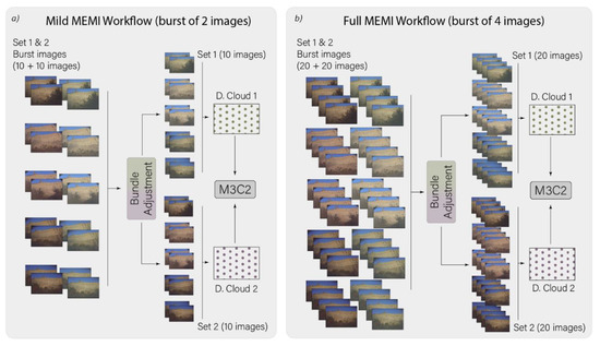
Figure 5.
(a) Mild MEMI workflow created for the change detection evaluation. (b) Full MEMI workflow created using all images available.
Comparison of the resulting 3D point cloud differences from the three workflows was carried out using the M3C2 from Lague et al. [43], implemented in the CloudCompare software. All comparisons (classic, MESI, mild MEMI and full MEMI) were performed using the same software configurations and images taken from the same modules at the same time but introducing more images from each burst the more complex the workflow. No filter was applied nor were any of the sparse point clouds considered differently. Although we used the same GCPs to geo-reference the images in all workflows, the point clouds obtained in the classic workflow needed to be aligned using the ICP algorithm [63] because set 1 and set 2 did not share exactly the same camera orientation due to the separate bundle adjustments.
2.5.2. Interior Precision of the Point Clouds
As well as considering the relative accuracy of change detection [1], we also assessed the interior precision of the retrieved 3D point clouds [1] with a test using the precision estimation algorithms described in James et al. [42]. The approach (Figure 6) allowed us to quantify the performance of the time-lapse SfM methods in a different way than the change detection test, presenting the spatial distribution of errors in terms of precision in centimetres and using a LiDAR TLS to retrieve ground control. For this test we used the images corresponding to November 8 and 13 because they were the most similar to the LiDAR TLS scan performed on October 2019. In 2019 the photogrammetric systems were not optimized to obtain bursts of four images, so the results presented were obtained using only bursts of three images, and with no separation into mild and full MEMI. Following the approach proposed by James et al. [42], the precision estimation values (σx σy σz) were estimated for each point of the sparse cloud. With a simple interpolation process, the precision estimation values (σx σy σz) were transferred from the sparse cloud points to the dense cloud points.
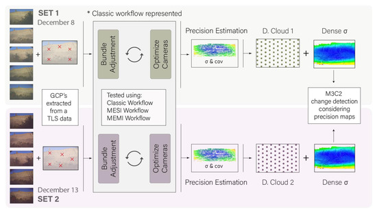
Figure 6.
Precision estimation to only detect significant changes. The 4D pipeline illustrated here comprises the classic workflow. The MESI and the MEMI workflow were also evaluated.
2.5.3. Absolute Accuracy of a Single Point Cloud
In order to determine the performance of the time-lapse SfM algorithms in terms of absolute accuracy, the final performance assessment consisted of comparing the photogrammetric models to LiDAR data. It was assumed that the LiDAR data represent a reference geometry, so the smaller the differences between the LiDAR and the photogrammetric models, the higher the absolute accuracy of them.
Due to the interval between the captured LiDAR data (October 2019) and the first captured photogrammetric data (November 2019), and the high number of rockfalls affecting the cliff, the period between datasets included several changes. In order to avoid eliminating the errors and smoothing of the results, the detected rockfalls were not eliminated for the absolute accuracy test. Therefore, this assessment does not represent a non-deformation scenario between the LiDAR data and the photogrammetric models.
3. Results
3.1. Relative Accuracy of Detected Changes
The differences between the two models of two consecutive days resulting from the MEMI workflow tended mostly to zero (Figure 7 and Figure 8), whereas the classic and MESI workflow revealed higher deviations, with the largest values measured with the former approach.
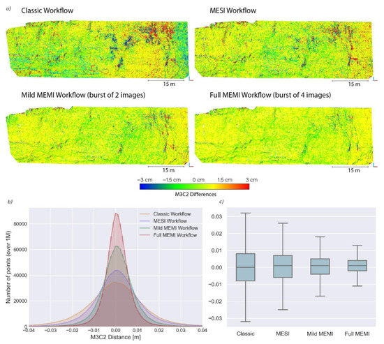
Figure 7.
(a) Graphic representation of the differences between the models of 23 and 24 May, according to the workflow used. The four models are represented using the same colour scale. (b) Histogram with the M3C2 results. (c) Error bar plot with the dispersion of the values obtained in each comparison.
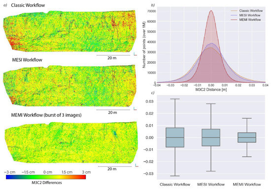
Figure 8.
(a) Graphic representation of the differences between the models of November 8 and 13, according to the workflow used. The three models are represented with the same colour scale. (b) Histogram with the M3C2 results. (c) Error bar plot with the dispersion of the values obtained in each comparison.
This can be observed in the maps of differences (Figure 7a) and in the histograms (Figure 7b) obtained using the May 2020 images. The smallest differences between the two compared days were achieved with the MEMI workflow using four images (full MEMI workflow). The standard deviation of the M3C2 differences decreased by 50%, from 3.37 cm in the classic workflow to 1.68 cm in the full MEMI workflow. The boxplots (Figure 7c) also highlight the increase in performance from classic to full MEMI, showing that both the average difference and the range of differences decreased.
The computational cost of each workflow as well as the main characteristics of the obtained models are described in Table 1.

Table 1.
Main parameters of the point clouds and M3C2 results obtained in May 2020 test.
Figure 8 also shows the M3C2 distance maps for the three different workflows (classic, MESI, MEMI), using the images captured in November 2019 to assess the relative accuracy of the point clouds (Figure 8a). The measured change detection with the MEMI workflow showed the lowest range of differences with respect to the other methods (Figure 8a). In addition, the histograms (Figure 8b) show a considerable reduction in the standard deviation of the differences (nearly 50%) when using MEMI, decreasing from 2.83 cm with the classic workflow to 1.54 cm with the MEMI workflow (Table 2).
Table 2.
Main parameters of the point clouds and M3C2 results obtained in November 2019 test.
3.2. Interior Precision of the Point Clouds
Figure 9 show the results obtained from the precision estimation test using the November 2019 images. Figure 9a shows the distribution of σy, which is the most important parameter for change detection in this study as it is the direction of highest deformation (depth direction). The results of the MEMI workflow show that precisions between 0 and 3 cm were concentrated in the central zone of the area of interest. Thus, this zone demonstrated the best photogrammetric reconstruction performance.
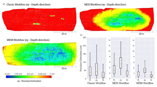
Figure 9.
(a) Results obtained from the precision estimation test, considering the distribution of σy (depth direction). (b) Error boxplots of the range of the precision estimations (note the different scale on the y axis).
With increasing distance from the central region (of highest image overlap) the precisions decreased in a spatial, radial-symmetric pattern. Similar patterns, but with higher magnitudes of precision, were identified in the MESI workflow. Such high values of σy were not obtained in the classic workflow, as shown in the error boxplots (Figure 9b). In general, the estimated precision of change detection was considerably higher with the MEMI workflow when compared to the classic and MESI approaches. The use of MEMI reduced both the error values as well as the range of these values along the escarpment, reaching σx and σz values below 2 cm (Table 3).
Table 3.
Main results obtained in the precision estimation test.
3.3. Absolute Accuracy of a Single Point Cloud
Figure 10 shows the M3C2 results obtained in the comparison of the three approaches described in Figure 4 in comparison to a reference LiDAR dataset. Figure 10a illustrates a small part of the cliff with the results of the M3C2 comparisons. Three images are represented using the same colour map.
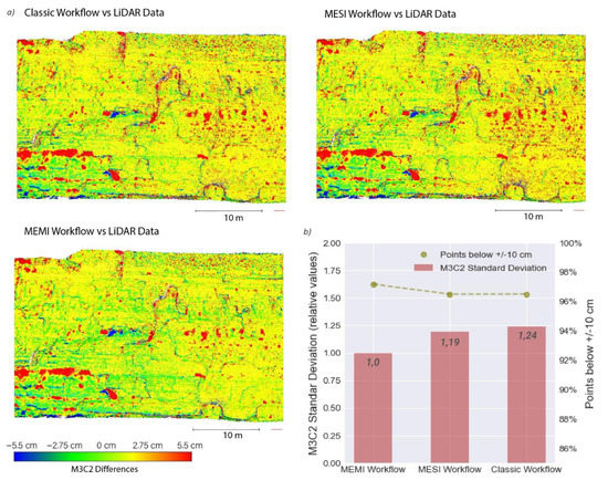
Figure 10.
(a) Graphic representation of the differences between the LiDAR data (October 2019) and photogrammetry models (November 2019), according to the workflow used. The three models are represented with the same colour map. The larger red clusters indicate rockfalls that occurred during the comparison period. (b) Bar plot showing the relative M3C2 standard deviation of the comparisons.
We observed that the MEMI vs. LiDAR data results showed lower random errors and that the detected rockfalls were better represented than in the classic or MESI results. In general, non-deformation zones (yellow and green) predominated in the MEMI comparison with respect to the other approaches. However, it should be noted that the best comparison was not error-free either, as very small clusters with false deformation were identified.
Due to the presence of rockfalls, the absolute standard deviation parameter does not represent a correct accuracy parameter. For this reason, Figure 10b shows the relative variation of the standard deviation with respect to the best comparison (MEMI vs. LiDAR data). The standard deviation of the M3C2 comparison increased by 19% when using the MESI algorithm and by 24% when using the classic workflow. Also, the graph in Figure 9b shows how the comparison with the highest points (97% of the points) within the range of +/−10 cm was the one made using the MEMI approach. The other workflows had lower values (close to 96%) which means that more points were in the range above +/−10 cm.
4. Discussion
4.1. Automated and Multi-Epoch Multi-Imagery (MEMI) Workflow
The results presented in this paper demonstrate a significant improvement in the methodology used to obtain automatic photogrammetric models using time-lapse cameras. The use of new methodologies such as the multi-epoch imagery (MESI) workflow already represents a considerable improvement in photogrammetric models as described in Feurer and Vinatier [25] and Cook and Dietze [1]. However, the multi-epoch multi-imagery (MEMI) workflow proposed in this paper allowed us to obtain photogrammetric models with greater geometric consistency and less error in the change detection comparison. So the comparison accuracy [1] was increased.
The main limitation of the pipeline presented in this paper is that it requires simultaneous photographs from the same locations during two different periods. So, it cannot be applied to images obtained by UAV, manual systems or historical pictures. A system of fixed cameras is required for the proper performance of the system. Although the cameras are installed in fixed systems of concrete the acquired images are not identical because there are variations in sensor position due to vibration, wind or temperature change, which is why it is necessary to apply automatic algorithms that allow one to track and obtain automatic GCP.
It should be noted that the results obtained in all performance assessments were obtained automatically using the entire pipeline proposed herein. The automation of the process increases the capacity for analysis and allows the data to be processed in a constant way in a server without the attention of an operator. And it overcomes one of the main limitations that exist when working with a great deal of data, which is being overwhelmed by the large amount of data. Overcoming this limitation is critical to 4D change detection work.
Focusing on the photogrammetric workflow presented in this paper we can define the enhanced workflow as a method for fixed cameras in which no lens calibration is required. Many articles have previously described the need for correct lens calibration. The results obtained using the classic method and MESI workflow reveal how part of the errors obtained have a dome effect classically associated with poor characterization of the intrinsic parameters of the camera. The MEMI workflow eliminates these errors thanks to the better characterization of the intrinsic parameters in the automatic lens calibration process performed by the photogrammetric software. All results have been obtained without any initial parameters developed based on a camera pre-calibration.
This improvement is possibly due to the redundancy of input data when solving the automatic calibration. However, the working method does not succeed in eliminating the classic limitations that all photogrammetric processes have. The quality of the model obtained decreases as we approach the extremes of the model because the photographic coverage of these points is more precarious. Also, in the shaded or poorly resolved areas of the images we find problems when making the photogrammetric reconstruction. The use of advanced methods does not end with the classic limitations of photogrammetry such as the loss of quality at the ends of the model but helps to mitigate its effects.
Despite the above limitations, the workflow presented allows the comparison of photogrammetric models with a better quality than using the classic method and allows work without lens calibration and without control points. These improvements simplify and facilitate the use of photogrammetric systems, especially in dangerous areas where it is impossible to reach the study area. A clear example of the application of this method is rockfall monitoring where it is impossible to access the cliff to install control points due to the danger of rockfall.
The results obtained in this study allow us to show both the improvements obtained using the multi-epoch single-imagery (MESI) workflow and the more advanced workflow multi-epoch multi-imagery (MEMI) developed in this work. The use of MESI workflows leads to an increase in accuracy and precision due to the fact that the spatial error behaviour is mitigated during change detection (i.e., by subtracting models and thus errors). Multi-imaging (from the same point in time) leads to increased accuracy and precision as the photons hit the sensor with a normal distribution and therefore slightly different image features are subsequently detected (leading to slightly different models); therefore, the more images the greater the consistency obtained in the bundle adjustment and consequently the higher the accuracy and precision. The synthesis of these two enhancement concepts is what produces the improvements we obtained for photogrammetric tracking systems from fixed time-lapse camera systems.
However, it should be noted that further work is needed to correctly identify which mechanism provides the best results. The use of proprietary software that works as a black box precludes us observing exactly which part of the processing is affected by the use of multi-imagery. Although the improvement in the results obtained is evident, why the use of multi-imaging has an impact on the results cannot be perfectly explained using our research.
4.2. Relative Accuracy of Detected Changes
One of the methods used in this paper to present the workflow improvements is a change detection analysis between photogrammetric models obtained on consecutive days. Working with photographs obtained on consecutive (or almost consecutive) days allows us to assume that there are no significant differences between the models and consequently that the change detection comparison should be close to 0. Moreover, this type of comparison allows us to quickly determine the errors that occur in the reconstruction process.
For this publication, two change detection tests were performed. The first test used the best possible data, using a burst of images of four photographs from two consecutive days in May 2020. The second test used the earliest available images (and closest to TLS data) captured on two close dates in November 2019. In this configuration only bursts of three photos were available. The M3C2 method, widely used in the quantification of differences in photogrammetric models, was used to eliminate non-representative deformation errors in comparisons of two point clouds.
In both tests (Figure 7 and Figure 8) we can see graphically how the differences obtained tended to zero when we used a MEMI workflow. These graphic observations were corroborated by the analysis of histograms. Both histograms showed that the classic workflow accumulated fewer points near zero with a greater dispersion of differences. On the other hand, the MEMI workflow accumulated many more points near the zero-deformation value and produced histograms with a lower dispersion of values. The evolution of these values can also be observed in the error bar plot of Figure 7c and Figure 8c. Figure 7c shows that when using the MEMI workflow with a burst of two images per position (mild MEMI workflow) the results obtained contained smaller geometric errors than when using the classic method or the multi-epoch single-imagery described by Feurer and Vinatier [25].
The results shown in Figure 7 and Figure 8 were obtained from different input data. Both figures show how the comparison accuracy improved with the pipeline presented in this article, reaching M3C2 standard deviations of around 1.5 cm. The improvement in the comparison accuracy is a relevant factor since it allows one to reduce the threshold in the detection of changes, increasing the ability to identify changes in the photogrammetric models studied. However, both figures also show how in the areas farthest from the centre there is a tendency to accumulate errors. These errors were mitigated in the more complex workflows, but they did not disappear. This suggests that these are areas where the identification of homologous points is poor, and the reconstruction of the model does not achieve the same quality.
In future works, it would be of great interest to test the performance of the MEMI algorithm in scenarios with larger differences between captures in order to determine whether the accuracies obtained in non-deformation scenarios are valid in scenarios where there are significant changes.
4.3. Interior Precision of the Point Clouds
In order to determine the interior precision of the point clouds, GCP was used to quantify precision at the real scale. However, the working method presented in this paper does not necessarily require control points since the resulting models for comparison share the same location of cameras and are perfectly positioned between them. It is interesting to note that the use of this workflow eliminates the tedious alignment process between point clouds. Because we work with fixed cameras, we can use GPS to obtain the location of each sensor, allowing the photogrammetric software to provide a georeferenced model without the need to use GCP control points, or we can align the locations with georeferenced data. However, the use of GCP allows better georeferencing as well as the possibility of implementing control points.
To calculate the precision we took advantage of the methodology developed by James et al. [42], which allowed us to obtain precision parameters from the control points that were used in the model. In the graphic visualization (Figure 9a) we can see the evolution of σy (parameters that indicate the precision in the direction of the deformation). Obtaining these values is subject to the precision of the GCPs introduced in the bundle adjustment phase. It should be remembered that for this work the GCPs were extracted from the local coordinates of a LiDAR TLS 3D model, so the precision obtained in the GCP extraction was not particularly high.
However, we are publishing these results with the intention of showing the progression of the estimation precision within the different workflows, as the same GCPs were used for all cases. We do not wish to focus on the absolute results, but rather on the fact that the comparison is relevant in relative terms. For this reason, Figure 9b shows how values were reduced considerably as more complex workflows were used.
Although obtaining the coordinates of the control points must be done in a more robust way, achieving precision values of less than 2 centimetres on the x and z axes and close to 3 centimetres on the y axis is remarkable. This precision estimation test represents a good way of expressing the improvement in real precision obtained using the MEMI workflow shown in this study.
4.4. Absolute Accuracy of a Single Point Cloud
The results obtained in the comparison of the different photogrammetric workflows with a LiDAR point cloud confirm the improvement that the MEMI workflow represents. It should be noted that the results do not show a perfect non-deformation comparison because there was a one-month difference between the LiDAR acquisition and the photogrammetric models.
This temporal gap is the reason why, in the comparison, in addition to obvious erroneous clusters, obvious rockfalls were identified as shown in Figure 10a. It should also be noted that the identification of rockfalls was much more reliable in the MEMI comparison than in the other workflows tested.
Due to the presence of rockfalls, the absolute values obtained are not representative of the absolute accuracy of the method. For this reason, the results are expressed in relative terms (Figure 10b). Both the graphical comparison and the relative quantification of the M3C2 standard deviation demonstrate that the use of the MEMI workflow substantially improves the absolute accuracy.
The use of multi-temporal multi-imaging algorithms minimizes the geometric error, yielding a 3D model much more similar to the one obtained by LiDAR (perfect in geometric terms). Furthermore, the improvement in absolute accuracy was due to the use of multi-images, as the differences between the classic workflow and the MEMI were not as clear. However, future work in which LiDAR data and photographs can be obtained simultaneously (non-deformation between LiDAR model and photogrammetric model) will allow the absolute accuracy of the different working methods proposed in this research to be achieved in a much more robust way.
5. Conclusions
Five autonomous fixed photogrammetric time-lapse systems were developed using conventional cameras controlled by microcontrollers. These systems allow photogrammetric models to be obtained and sent autonomously and with a high-temporal resolution (sub-daily basis) allowing 4D analysis. The comparison made with the classic, multi-epoch single-imagery (MESI) and multi-epoch multi-imagery (MEMI) workflows shows that the workflow developed in this article leads to significant improvements in the construction of photogrammetric models. The improvements demonstrated in this paper yield models with a greater geometric coherence between them without the need for complex camera calibrations, post-process alignments or the use of GCPs. The MEMI workflow reduced the error up to a factor of 2 in the comparison accuracy (2.83 cm with the classic workflow vs. 1.54 cm with the proposed approach). The proposed enhancement is very relevant when performing studies based on change detection processes. The published pipeline reduces the deformation thresholds used to determine if changes have occurred. Finally, our work shows the possibility of automating the entire workflow without any user intervention, demonstrating that there is the possibility of developing automatic systems for control and monitoring of surfaces via the use of photogrammetric systems.
Author Contributions
Algorithm conceptualization and methodology: X.B., A.E.; software: X.B., A.E.; formal analysis: X.B., A.E., M.G. and A.A., investigation: X.B., A.E., M.G. and A.A., validation: X.B., A.E. M.G. and A.A. writing—original draft preparation, X.B.; writing—review and editing A.E., M.G., A.A.; visualization: X.B.; supervision, A.E., M.G. and A.A. All authors have read and agreed to the published version of the manuscript.
Funding
The presented study was supported by the PROMONTEC Project (CGL2017-84720-R) funded by the Ministry of Science, Innovation and Universities (MICINN-FEDER). The first author (X. Blanch) was supported by an APIF grant funded by the University of Barcelona and the second author (A. Abellán) was supported by the European Union’s Horizon 2020 research and innovation programme under a Marie Skłodowska-Curie fellowship (grant agreement no. 705215). Anette Eltner was funded by the DFG (EL 926/3-1).
Data Availability Statement
The data (image sets) that support the findings of this study are available from the corresponding author, upon reasonable request.
Acknowledgments
The authors would like to thank Mike James for his help and support in the precision estimation results, the ORIGENS UNESCO Global Geopark for granting permission to work on Puigcercós rock cliff and the reviewers and the editor for the valuable comments and suggestions that contributed to the improvement of the present manuscript.
Conflicts of Interest
The authors declare no conflict of interest.
References
- Cook, K.L.; Dietze, M. Short communication: A simple workflow for robust low-cost UAV-derived change detection without ground control points. Earth Surf. Dyn. Discuss. 2019, 1–15. [Google Scholar] [CrossRef]
- Bartonek, D.; Buday, M. Problems of creation and usage of 3D model of structures and theirs possible solution. Symmetry 2020, 12, 181. [Google Scholar] [CrossRef]
- Meidow, J.; Usländer, T.; Schulz, K. Obtaining as-built models of manufacturing plants from point clouds. At-Automatisierungstechnik 2018, 66. [Google Scholar] [CrossRef]
- Artese, S.; Lerma, J.L.; Zagari, G.; Zinno, R. The survey, the representation and the structural modeling of a dated bridge. In Proceedings of the 8th International Congress on Archaeology, Computer Graphics, Cultural Heritage and Innovation, Valencia, Spain, 5–7 September 2016; Universitat Politecnica de Valencia: Valencia, Spain, 2016. [Google Scholar]
- Castellazzi, G.; D’Altri, A.M.; Bitelli, G.; Selvaggi, I.; Lambertini, A. From laser scanning to finite element analysis of complex buildings by using a semi-automatic procedure. Sensors 2015, 15, 8360. [Google Scholar] [CrossRef] [PubMed]
- Jaboyedoff, M.; Oppikofer, T.; Abellán, A.; Derron, M.H.; Loye, A.; Metzger, R.; Pedrazzini, A. Use of LIDAR in landslide investigations: A review. Nat. Hazards 2012, 61, 5–28. [Google Scholar] [CrossRef]
- Abellán, A.; Oppikofer, T.; Jaboyedoff, M.; Rosser, N.J.; Lim, M.; Lato, M.J. Terrestrial laser scanning of rock slope instabilities. Earth Surf. Process. Landf. 2014, 39, 80–97. [Google Scholar] [CrossRef]
- Eltner, A.; Schneider, D. Analysis of different methods for 3D reconstruction of natural surfaces from parallel-axes UAV images. Photogramm. Rec. 2015, 30, 279–299. [Google Scholar] [CrossRef]
- Eltner, A.; Kaiser, A.; Castillo, C.; Rock, G.; Neugirg, F.; Abellán, A. Image-based surface reconstruction in geomorphometry-merits, limits and developments. Earth Surf. Dyn. 2016, 4, 359–389. [Google Scholar] [CrossRef]
- Westoby, M.J.; Brasington, J.; Glasser, N.F.; Hambrey, M.J.; Reynolds, J.M. “Structure-from-Motion” photogrammetry: A low-cost, effective tool for geoscience applications. Geomorphology 2012, 179, 300–314. [Google Scholar] [CrossRef]
- Anderson, K.; Westoby, M.J.; James, M.R. Low-budget topographic surveying comes of age: Structure from motion photogrammetry in geography and the geosciences. Prog. Phys. Geogr. 2019, 43, 163–173. [Google Scholar] [CrossRef]
- James, M.R.; Robson, S. Straightforward reconstruction of 3D surfaces and topography with a camera: Accuracy and geoscience application. J. Geophys. Res. Earth Surf. 2012, 117, 1–17. [Google Scholar] [CrossRef]
- Blanch, X.; Abellan, A.; Guinau, M. Point cloud stacking: A workflow to enhance 3D monitoring capabilities using time-lapse cameras. Remote Sens. 2020, 12, 1240. [Google Scholar] [CrossRef]
- Micheletti, N.; Chandler, J.H.; Lane, S.N. Investigating the geomorphological potential of freely available and accessible structure-from-motion photogrammetry using a smartphone. Earth Surf. Process. Landf. 2015, 40, 473–486. [Google Scholar] [CrossRef]
- Eltner, A.; Sofia, G. Structure from motion photogrammetric technique. Dev. Earth Surf. Process. 2020, 23, 1–24. [Google Scholar] [CrossRef]
- Kromer, R.; Walton, G.; Gray, B.; Lato, M.; Group, R. Development and optimization of an automated fixed-location time lapse photogrammetric rock slope monitoring system. Remote Sens. 2019, 11, 1890. [Google Scholar] [CrossRef]
- Giacomini, A.; Thoeni, K.; Santise, M.; Diotri, F.; Booth, S.; Fityus, S.; Roncella, R. Temporal-spatial frequency rockfall data from open-pit highwalls using a low-cost monitoring system. Remote Sens. 2020, 12, 2459. [Google Scholar] [CrossRef]
- Verma, A.K.; Bourke, M.C. A method based on structure-from-motion photogrammetry to generate sub-millimetre-resolution digital elevation models for investigating rock breakdown features. Earth Surf. Dyn. 2019, 7, 45–66. [Google Scholar] [CrossRef]
- Gaffey, C.; Bhardwaj, A. Applications of unmanned aerial vehicles in cryosphere: Latest advances and prospects. Remote Sens. 2020, 12, 948. [Google Scholar] [CrossRef]
- Tannant, D. Review of photogrammetry-based techniques for characterization and hazard assessment of rock faces. Int. J. Geohazards Environ. 2015, 1, 76–87. [Google Scholar] [CrossRef]
- Nesbit, P.R.; Hugenholtz, C.H. Enhancing UAV-SfM 3D model accuracy in high-relief landscapes by incorporating oblique images. Remote Sens. 2019, 11, 239. [Google Scholar] [CrossRef]
- Nex, F.; Remondino, F. UAV for 3D mapping applications: A review. Appl. Geomat. 2014, 6, 1–15. [Google Scholar] [CrossRef]
- Liu, W.; Wang, C.; Zang, Y.; Lai, S.H.; Weng, D.; Sian, X.; Lin, X.; Shen, X.; Li, J. Ground camera images and UAV 3D model registration for outdoor augmented reality. In Proceedings of the 26th IEEE Conference on Virtual Reality and 3D User Interfaces, VR 2019, Osaka, Japan, 23–27 March 2019. [Google Scholar]
- Wu, Z.; Ni, M.; Hu, Z.; Wang, J.; Li, Q.; Wu, G. Mapping invasive plant with UAV-derived 3D mesh model in mountain area—A case study in Shenzhen Coast, China. Int. J. Appl. Earth Obs. Geoinf. 2019, 77. [Google Scholar] [CrossRef]
- Feurer, D.; Vinatier, F. Joining multi-epoch archival aerial images in a single SfM block allows 3-D change detection with almost exclusively image information. ISPRS J. Photogramm. Remote Sens. 2018, 146, 495–506. [Google Scholar] [CrossRef]
- Parente, L.; Chandler, J.H.; Dixon, N. Optimising the quality of an SfM-MVS slope monitoring system using fixed cameras. Photogramm. Rec. 2019, 34, 408–427. [Google Scholar] [CrossRef]
- Roncella, R.; Forlani, G.; Fornari, M.; Diotri, F. Landslide monitoring by fixed-base terrestrial stereo-photogrammetry. ISPRS Ann. Photogramm. Remote Sens. Spat. Inf. Sci. 2014, 2, 297–304. [Google Scholar] [CrossRef]
- Motta, M.; Gabrieli, F.; Corsini, A.; Manzi, V.; Ronchetti, F.; Cola, S. Landslide Displacement Monitoring from Multi-Temporal Terrestrial Digital Images: Case of the Valoria Landslide Site. In Landslide Science and Practice; Margottini, C., Canuti, P., Sassa, K., Eds.; Springer: Berlin/Heidelberg, Germany, 2013; Volume 2, pp. 73–78. [Google Scholar]
- Raspberry Pi Foundation. Raspberry Pi 3 Model B. 2016. Available online: https://www.raspberrypi.org/ (accessed on 1 April 2020).
- Eltner, A.; Elias, M.; Sardemann, H.; Spieler, D. Automatic image-based water stage measurement for long-term observations in ungauged catchments. Water Resour. Res. 2018, 54, 10362–10371. [Google Scholar] [CrossRef]
- Santise, M.; Thoeni, K.; Roncella, R.; Sloan, S.W.; Giacomini, A. Preliminary tests of a new low-cost photogrammetric system. Int. Arch. Photogramm. Remote Sens. Spat. Inf. Sci. ISPRS Arch. 2017, 42, 229–236. [Google Scholar] [CrossRef]
- Mallalieu, J.; Carrivick, J.L.; Quincey, D.J.; Smith, M.W.; James, W.H.M. An integrated structure-from-motion and time-lapse technique for quantifying ice-margin dynamics. J. Glaciol. 2017, 63, 937–949. [Google Scholar] [CrossRef]
- Ntregka, A.; Georgopoulos, A.; Quintero, M.S. Photogrammetric exploitation of hdr images for cultural heritage documentation. ISPRS Ann. Photogramm. Remote Sens. Spat. Inf. Sci. 2013, 2, 209–214. [Google Scholar] [CrossRef]
- Gómez-Gutiérrez, Á.; de Sanjosé-Blasco, J.J.; Lozano-Parra, J.; Berenguer-Sempere, F.; de Matías-Bejarano, J. Does HDR pre-processing improve the accuracy of 3D models obtained by means of two conventional SfM-MVS software packages? The case of the corral del veleta rock glacier. Remote Sens. 2015, 7, 10269–10294. [Google Scholar] [CrossRef]
- Romeo, S.; di Matteo, L.; Kieffer, D.S.; Tosi, G.; Stoppini, A.; Radicioni, F. The use of gigapixel photogrammetry for the understanding of landslide processes in alpine terrain. Geosciences 2019, 9, 99. [Google Scholar] [CrossRef]
- Lato, M.J.; Bevan, G.; Fergusson, M. Gigapixel imaging and photogrammetry: Development of a new long range remote imaging technique. Remote Sens. 2012, 4, 3006–3021. [Google Scholar] [CrossRef]
- Guidi, G.; Gonizzi, S.; Micoli, L.L. Image pre-processing for optimizing automated photogrammetry performances. ISPRS Ann. Photogramm. Remote Sens. Spat. Inf. Sci. 2014, 2, 145–152. [Google Scholar] [CrossRef]
- James, M.R.; Robson, S. Mitigating systematic error in topographic models derived from UAV and ground-based image networks. Earth Surf. Process. Landf. 2014, 39, 1413–1420. [Google Scholar] [CrossRef]
- Luhmann, T.; Fraser, C.; Maas, H.G. Sensor modelling and camera calibration for close-range photogrammetry. ISPRS J. Photogramm. Remote Sens. 2016, 115, 37–46. [Google Scholar] [CrossRef]
- Elias, M.; Eltner, A.; Liebold, F.; Maas, H.G. Assessing the influence of temperature changes on the geometric stability of smartphone-and raspberry Pi cameras. Sensors 2020, 20, 643. [Google Scholar] [CrossRef] [PubMed]
- Eltner, A.; Kaiser, A.; Abellan, A.; Schindewolf, M. Time lapse structure-from-motion photogrammetry for continuous geomorphic monitoring. Earth Surf. Process. Landf. 2017, 42, 2240–2253. [Google Scholar] [CrossRef]
- James, M.R.; Robson, S.; Smith, M.W. 3-D uncertainty-based topographic change detection with structure-from-motion photogrammetry: Precision maps for ground control and directly georeferenced surveys. Earth Surf. Process. Landf. 2017, 42, 1769–1788. [Google Scholar] [CrossRef]
- Lague, D.; Brodu, N.; Leroux, J. Accurate 3D comparison of complex topography with terrestrial laser scanner: Application to the Rangitikei canyon (N-Z). ISPRS J. Photogramm. Remote Sens. 2013, 82, 10–26. [Google Scholar] [CrossRef]
- Hungr, O.; Leroueil, S.; Picarelli, L. The Varnes classification of landslide types, an update. Landslides 2014, 11, 167–194. [Google Scholar] [CrossRef]
- Vidal, L.M. Nota acerca de los hundimientos ocurridos en la Cuenca de Tremp (Lérida) en Enero de 1881. In Boletín de la Comisión del Mapa Geológico de España VIII; Imprenta Y Fundición de Manuel Tello: Madrid, Spain, 1881; pp. 113–129. [Google Scholar]
- Corominas, J.; Alonso, E. Inestabilidad de laderas en el Pirineo catalán. Ponen. Comun. ETSICCP-UPC C.1 C.53 1984. [Google Scholar]
- Abellán, A.; Calvet, J.; Vilaplana, J.M.; Blanchard, J. Detection and spatial prediction of rockfalls by means of terrestrial laser scanner monitoring. Geomorphology 2010, 119, 162–171. [Google Scholar] [CrossRef]
- Tonini, M.; Abellan, A. Rockfall detection from terrestrial LiDAR point clouds: A clustering approach using R. J. Spat. Inf. Sci. 2014, 8, 95–110. [Google Scholar] [CrossRef]
- Royán, M.J.; Abellán, A.; Jaboyedoff, M.; Vilaplana, J.M.; Calvet, J. Spatio-temporal analysis of rockfall pre-failure deformation using Terrestrial LiDAR. Landslides 2014, 11, 697–709. [Google Scholar] [CrossRef]
- Royán, M.J.; Abellán, A.; Vilaplana, J.M. Progressive failure leading to the 3 December 2013 rockfall at Puigcercós scarp (Catalonia, Spain). Landslides 2015, 12, 585–595. [Google Scholar] [CrossRef]
- Khazaradze, G.; Guinau, M.; Blanch, X.; Abellan, A.; Vilaplana, J.M.; Royan, M.; Tapia, M.; Roig, P.; Furdada, G.; Suriñach, E. Puigcercós: A natural laboratory to study landslides and rockfalls in the Catalan Pyrenees. Multi-scale analysis of Slopes under climate change. A cross-disciplinary work. MUSLOC 2019. [Google Scholar]
- Khazaradze, G.; Guinau, M.; Blanch, X.; Abellán, A.; Tapia, M.; Furdada, G.; Suriñach, E. Multidisciplinary studies of the Puigcercós historical landslide in the Catalan Pyrenees. Geophys. Res. Abstr. 2020, 22, 7796. [Google Scholar]
- Suriñach, E.; Tapia, M.; Roig, P.; Blanch, X. On the effect of the ground seismic characteristics in the estimation of mass movements based on seismic observation. Geophys. Res. Abstr. 2018, EGU8479, 20. [Google Scholar]
- Python Core Team. Python: A Dynamic, Open Source Programming Language. Python Software Foundation. 2020. Available online: https://www.python.org/ (accessed on 1 April 2020).
- Bradski, G. The OpenCV Library. Dr Dobbs J. Softw. Tools 2000. [Google Scholar] [CrossRef]
- Pech-Pacheco, J.L.; Cristöbal, G.; Chamorro-Martínez, J.; Fernândez-Valdivia, J. Diatom autofocusing in brightfield microscopy: A comparative study. Proc. Int. Conf. Pattern Recognit. 2000, 15, 314–317. [Google Scholar] [CrossRef]
- Pertuz, S.; Puig, D.; Garcia, M.A. Analysis of focus measure operators for shape-from-focus. Pattern Recognit. 2013, 46, 1415–1432. [Google Scholar] [CrossRef]
- Yilmaz, A.; Javed, O.; Shah, M. Object tracking: A survey. ACM Comput. Surv. 2006, 38, 13-es. [Google Scholar] [CrossRef]
- Schwalbe, E.; Maas, H.-G. Determination of high resolution spatio-temporal glacier motion fields from time-lapse sequences. Earth Surf. Dyn. Discuss. 2017, 1–30. [Google Scholar] [CrossRef]
- Lucas, B.D.; Kanade, T. Iterative image registration technique with an application to stereo vision. In Proceedings of the 7th International Joint Conference on Artificial Intelligence (IJCAI), Vancouver, BC, Canada, 24–28 August 1981; Volume 2, pp. 674–679. [Google Scholar]
- Baker, S.; Matthews, I. Lucas-Kanade 20 years on: A unifying framework. Int. J. Comput. Vis. 2004, 56, 221–255. [Google Scholar] [CrossRef]
- Lin, D.; Grundmann, J.; Eltner, A. Evaluating image tracking approaches for surface velocimetry with thermal tracers. Water Resour. Res. 2019, 55, 3122–3136. [Google Scholar] [CrossRef]
- Chen, Y.; Medioni, G.G. Object modelling by registration of multiple range images. Image Vis. Comput. 1992, 10, 145–155. [Google Scholar] [CrossRef]
- Agisoft Metashape Professional Edition (Version 1.6.6). Software. 2020. Available online: http://www.agisoft.com/downloads/installer/ (accessed on 1 April 2020).
- Agisoft LLC. Metashape Python Reference, Release 1.6.0; Agisoft LLC: Petersburg, Russia, 2018; pp. 1–199. [Google Scholar]
- CloudCompare (Version 2.11). 2021. Available online: http://www.cloudcompare.org/ (accessed on 1 April 2020).
- Ester, M.; Kriegel, H.P.; Sander, J.; Xu, X. A density-based algorithm for discovering clusters in large spatial databases with noise. Kdd 1996, 96, 226–231. [Google Scholar] [CrossRef]
Publisher’s Note: MDPI stays neutral with regard to jurisdictional claims in published maps and institutional affiliations. |
© 2021 by the authors. Licensee MDPI, Basel, Switzerland. This article is an open access article distributed under the terms and conditions of the Creative Commons Attribution (CC BY) license (https://creativecommons.org/licenses/by/4.0/).