Abstract
Water detection algorithms are now being routinely applied to continental and global archives of satellite imagery. However, water resource management decisions typically take place at the waterbody rather than pixel scale. Here, we present a workflow for generating polygons of persistent waterbodies from Landsat observations, enabling improved monitoring and management of water assets across Australia. We use Digital Earth Australia’s (DEA) Water Observations from Space (WOfS) product, which provides a water classified output for every available Landsat scene, to determine the spatial locations and extents of waterbodies across Australia. We generated a polygon set of waterbodies that identified 295,906 waterbodies ranging in size from 3125 m2 to 4820 km2. Each polygon was used to generate a time series of WOfS, providing a history of the change in surface area of each waterbody every ~16 days since 1987. We demonstrate the applications of this new dataset, DEA Waterbodies, to understanding local through to national-scale surface water spatio-temporal dynamics. DEA Waterbodies provides new insights into Australia’s water availability and enables the monitoring of important landscape features such as lakes and dams, improving our ability to use earth observation data to make meaningful decisions.
1. Introduction
Water availability and security is a key consideration for humans and natural ecosystems world-wide. Competing demands for limited water resources between human consumptive use and ecosystems is already placing many natural systems under stress [1,2,3,4,5]. Water resource conflicts between neighbouring nations are already occurring, and these conflicts are likely to worsen as climate change increases the uncertainty in rainfall and evapotranspiration [6,7,8].
In Australia, the world’s driest inhabited continent, water availability is a key social, environmental and economic issue affecting the lives of millions of Australians. Australia has an extensive surface water monitoring network in place, consisting of stream gauges and publicly owned water storage monitoring. While these surface monitoring networks consist of tens of thousands of instruments, Australia’s large land area and ephemeral surface water mean that large parts of its surface water network remain unmetered.
Multi-decadal archives of satellite imagery provide insight into water resource availability in two key ways. Firstly, they have the ability to map and monitor catchment-wide and continent-wide surface water dynamics, supplementing or replacing surface networks in data-sparse regions [9,10,11]. Secondly, the multi-decadal perspective of these archives means that the changes in surface water that are currently taking place can be placed into the context of historical surface water dynamics [12,13]. Satellite data from public-good satellites such as the Landsat series are freely available and global in coverage [14,15,16], facilitating global-scale analysis of inland surface water [12,13,17,18]. Australia-specific surface water studies have also been carried out, which detect the frequency of water across the landscape [19,20], as well as map the locations of seasonal and permanent waterbodies [21,22].
Whilst information about the presence/absence of water provides valuable insight into multi-decadal surface water dynamics, further analysis is required to make the information content more accessible to water managers. This is because water management decisions are typically based on waterbodies (dams, lakes, river reaches, refugial pools) rather than pixels. Waterbody mapping with satellite imagery has almost exclusively been done on a pixel-by-pixel [12,13,18,20,21,23,24] (or sub-pixel [25,26,27,28] basis), with only a few studies delineating waterbodies as vector objects [29,30,31,32]. The delineation of waterbodies provides an object-based analysis, which characterises the dynamics of the whole waterbody, not its individual pixels. This allows analysis of waterbody characteristics such as the change in surface area over time [24,33], facilitating study of the events observed to be impacting individual waterbodies [33]. This in turn allows environmental water managers to evaluate the efficacy of environmental flow events in providing aquatic ecosystem provision objectives [34].
Analysing surface water dynamics with respect to individual waterbodies depends on the availability of a waterbody polygon set. In previous studies waterbody polygons have been generated from pre-existing cartographic coverages [35], or from a select number of cloud-free images [31,36]. The key limitation of these approaches is that the polygon sets are dependent on line work derived from either a single point in time [35] or reference imagery from a narrow range of dates [31,36]. This limits the ability of these approaches to identify ephemeral or recently formed waterbodies.
The combination of ‘analysis ready data’ [37] with large scale Earth observation analytics platforms such as Google Earth Engine [38] and Open Data Cube [39] now make it possible to analyse all available water observations to derive a waterbody polygon set.
The aim of this paper is to describe the use of Digital Earth Australia (the Australian instance of Open Data Cube) [39] to identify inland waterbodies across Australia and to characterise the change in their surface area from 1987–2018 for the purposes of providing river regulators, environmental water managers, agricultural water users and catchment managers with a common, transparent, and shared understanding of Australia’s surface water resources. The specific objectives are to:
- Use Water Observations from Space (WOfS) [19] inundation frequency from 1987–2018 to generate waterbody polygons delineating each waterbody’s maximum surface extent over this period.
- Quantify the time series of water surface area for each polygon for all available Landsat observations (1987–present).
- Demonstrate how these polygon-specific time series can be aggregated to provide insight into water availability.
The DEA Waterbodies interface is publicly available via DEA Maps (https://maps.dea.ga.gov.au/, accessed on 31 March 2021), ensuring that routine, robust, and repeatable information about Australia’s waterbodies remains current and openly available.
2. Materials and Methods
2.1. Study Area
Australia is the driest inhabited continent on Earth. Australia’s climate spans Koppen climate zones from tropical rainforest to hot desert and temperate climates (Figure 1). Australia experiences highly variable rainfall patterns driven by multiple large-scale climate drivers [40] as well as shorter-lived weather events [41,42]. The amount of surface water across the Australian continent at any point in time is hard to determine, however some estimates exist from remotely sensed data [19,43] and surface hydrology networks [44].
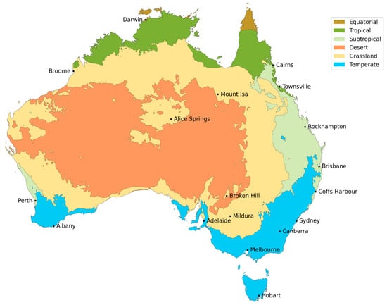
Figure 1.
Koppen climate classification of Australia adapted from [45].
2.2. Satellite Imagery
DEA is a data platform created within Geoscience Australia that generates analysis-ready satellite data that can be used to monitor changes in Australia’s land surface over time [39,46]. DEA provides free and open earth observation data from two public-good satellite programs: Landsat [47] and Sentinel 2 [48]. The Landsat program, operated by the United States Geological Survey and National Aeronautics and Space Administration (NASA), consists of three multi-spectral satellites/sensors: Landsat 5 TM (1984–2013), Landsat 7 ETM+ (1999–present), and Landsat 8 OLI (2013–present). These sensors have a 30 m pixel resolution, and image the Earth every 16 days on average. Landsat 5 TM was operational from 1984, however routinely collected data from 1987 to 2011, before being decommissioned in 2013 [49]. The Landsat 7 ETM+ and Landsat 8 OLI missions are still operational, however a failure of the scan-line corrector in Landsat 7 ETM+ in May 2003 means that imagery acquired by the satellite after this date has stripes of missing data, as no gap-fill algorithm is applied to this data. These missing data have some effect on the overall quality of the data from this satellite, however the data present can still provide valuable insights into surface changes across Australia [50], particularly when combined with data from Landsat 8 OLI.
The raw satellite data from the Landsat missions have been corrected, standardised, and orthorectified to produce an archive of analysis-ready data at 25 m pixel resolution [39,46]. This data can be accessed using the Open Data Cube API [51] via DEA, allowing automatic extraction and processing of the Earth observation archives.
2.3. Water Observations from Space (WOfS)
Water Observations from Space (WOfS) is a water detection algorithm that classifies each cloud-masked, observed pixel into wet, dry or invalid (i.e., cloud obscured, high slope) for all available observations through time [19]. WOfS uses a decision tree based on a series of Landsat band ratios and ancilliary datasets such as valley bottom flatness and pixel quality. This additional information provides an extra degree of validation for the decision tree classifications, over more basic band ratio water classifiers like the normalised difference water index (NDWI).
The WOfS classifier has a high overall degree of accuracy (97%) in correctly classifying the presence of water, however this accuracy decreases where there are water and other targets, particularly vegetation, occurring within the same pixel. WOfS is most effective where there is a clear, unobstructed water surface that has been sampled by the satellites, and is known to misclassify areas where water and vegetation co-exist as dry, such as wetlands and riparian zones.
WOfS is run on the Landsat archive by DEA, providing a 32-year history of water classified pixels for all of Australia. We make use of this archive to identify where pixels have been frequently mapped as wet using the WOfS classifier to generate a map of surface waterbodies across Australia.
3. Workflow
Our methodology takes advantage of WOfS data within DEA to locate and extract information about persistent waterbodies across Australia. The workflow is written in Python, and has been almost completely automated to minimise subjective decision making and ensure reproducibility, allowing the workflow to be run repeatedly with the same outcome. The code used to produce DEA Waterbodies is open source, and provided for use under an Apache Licence, Version 2.0 (see Appendix A).
The workflow is built off the WOfS Statistics dataset [52]. The WOfS Statistics dataset provides a pixel-by-pixel count of clear observations (i.e., not impacted by cloud, cloud shadow, or other satellite acquisition issues), wet observation counts (total number of times a pixel was observed as wet over the archive period), and a frequency statistic that provides the number of wet observations as a percentage of the number of clear observations over the period 1987–2018. The frequency statistic provides an indicator of how often water is observed in each pixel over this time period, and it is this product that forms the basis of this workflow.
In order to turn the WOfS frequency statistic into automatically generated polygons of waterbody locations, a series of steps need to be applied to remove erroneous data, and to map only the areas of water that meet specified thresholds. The decision tree used to produce DEA Waterbodies is shown in Figure 2. A detailed description of the methodology is included in Appendix A.
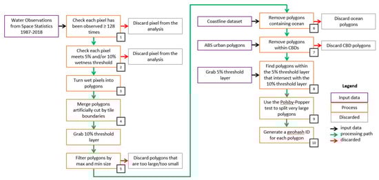
Figure 2.
DEA Waterbodies workflow diagram. For a detailed description of the steps involved in producing the waterbody polygons, see Appendix A.
The workflow for DEA Waterbodies consists of ten steps:
- Check each pixel has been observed ≥128 times over the period 1987–2018 (equates to at least four observations per year of analysis) to exclude pixels that are very infrequently observed.
- Check each pixel meets a wet frequency threshold, to define waterbodies only where water persists in the landscape. We used two thresholds to generate two wet layers: 5% and 10%. These two thresholds were used in combination to ensure that infrequently inundated portions of larger waterbodies were included in the final polygons (see Appendix A).
- Turn wet pixels into polygons. This facilitates an object-based, rather than a pixel-based analysis.
- Merge polygons artificially cut by tile boundaries. Tile boundaries are an artefact of the way the data are stored and adjoining waterbodies need to be connected.
- Filter polygons by minimum size. We applied a five Landsat pixel (25 by 25 m) minimum size limit (3125 m2).
- Remove polygons containing ocean. We applied a custom ocean mask to remove ocean and ocean-connected waterbodies from the final dataset.
- Remove polygons within city centres. The WOfS classifer can mistake deep shadows from high-rise buildings for water, so we remove any waterbodies identified within high-rise city regions.
- Find polygons within the 5% wet frequency threshold layer that intersect with the 10% wet frequency threshold layer. The locations of the waterbody polygons are defined by the 10% wet frequency threshold, but the extent of the polygon is defined by the 5% wet frequency threshold.
- Use the Polsby–Popper test [53] to identify and manually split very large polygons. The Polsby–Popper statistic was used as an objective means of identifying very long and/or complicated polygons for manual curation.
- Generate a geohash identifier for each polygon. A geohash was used to generate a unique identifier for each mapped waterbody polygon.
The resulting waterbody polygon dataset represents the maximum extent of waterbodies across the Australian landscape from 1987–2018. The wet frequency thresholds have been chosen to include locations that are infrequently, but repeatedly wet, while excluding short-lived and infrequent events like flash flooding (see Appendix A).
4. Time Series Extraction for Each Polygon
Each individual waterbody polygon was interrogated to return a time series of wet surface area through time. The WOfS classifier can be run on individual Landsat scenes to get a snapshot of water/not water for every satellite acquisition since 1987. We used the waterbodies dataset to perform polygon drills, whereby the individual waterbody polygons were used to ‘drill’ through the stack of water classified Landsat imagery through time, to produce a 32-year history of water surface area (Figure 3). Only scenes where at least 80% of the total waterbody was clearly observed were included to minimise erroneous results caused by cloud, Landsat 7 scan-line off missing values or swath boundaries. Each waterbody time series provides insights into the percentage of each total polygon area that is observed as wet for each satellite observation. Given that the waterbody polygons represent a maximum area for each waterbody, it is common for only part of the whole polygon to be observed as wet. Depending on the shape and nature of each polygon, some polygons will regularly be observed as 100% wet area or 100% dry area (e.g., constructed on-farm storages), while some polygons will never be completely dry (e.g., most large water reservoirs) or completely wet (e.g., large inland lakes like Kati Thanda–Lake Eyre).
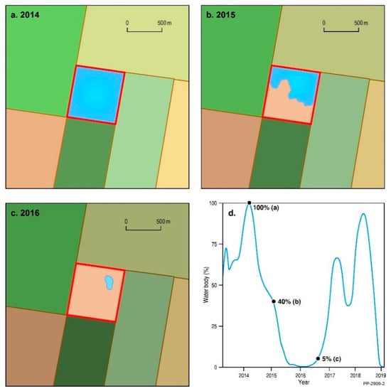
Figure 3.
Conceptualisation of the time series extraction for each polygon. (a–c) At each individual time step, the percentage surface area of water (indicated in blue) within each waterbody polygon (outlined in red) was calculated, producing a time series (d) of the change in surface water extent for each waterbody since 1987.
The time series associated with each waterbody is stored in a separate CSV file, named according to the polygon geohash. Each CSV file is updated as new WOfS data become available, providing an operational picture of the changing wet surface area of each waterbody over time.
Due to the 2D nature of satellite imagery, this information is only available for surface area, and not for waterbody volume. For steep-sided waterbodies (for example, constructed water storages), a negligible change in surface area may equate to a large change in total waterbody volume. Despite this, the surface area change in water extent provides powerful insights into the timing of filling and emptying events.
5. Results
5.1. Validation
5.1.1. Polygon Validation
We compared polygons from DEA Waterbodies to those from the Bureau of Meteorology Australian Hydrological Geospatial Fabric (Geofabric). The Geofabric is Australia’s most comprehensive hydrological cartography product: a digital database of surface and groundwater hydrological features, including the spatial relationships between them [54]. It is described as a ‘digital street directory of Australia’s important water features’ ([55], p. 2). Waterbody polygons contained within the Geofabric are taken from the Surface Hydrology Database [56], which is composed of datasets from state government agencies from satellite imagery, aerial imagery, fieldwork, digital elevation models and other data sources. The Geofabric represents the best available, nationally recognised and extensively quality controlled dataset of Australian waterbodies, and as such, is the most suitable dataset for validation of DEA Waterbodies polygons.
The overall distribution of waterbody size is very similar between DEA Waterbodies and the Geofabric. DEA Waterbodies misses waterbodies smaller than 5 Landsat pixels (3125 m2) which we explicitly filtered out (Figure 4). However, DEA Waterbodies maps more small waterbodies above this threshold. There are likely two reasons for this: first, complex waterbody boundaries may result in many small discrete waterbodies, rather than a single object; second, DEA Waterbodies identifies additional new waterbodies not mapped in the Geofabric. Other discrepancies may come from the different methods by which the products were created: waterbodies mapped in DEA Waterbodies must have been observed to be wet in at least 10% of observations since 1987, as opposed to Geofabric waterbodies, which are visually interpreted and may be no longer active or may not have existed at the time of production.
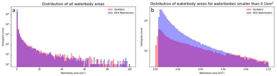
Figure 4.
Size distribution of waterbodies in DEA Waterbodies and the Geofabric for (a) all waterbodies, (b) waterbodies less than 0.1 km2.
We also performed a closer comparison on two regions, one near Moree NSW with well-defined but dynamic farm dams, and one area dominated by salt lakes near Cranbrook WA. The comparison between DEA Waterbodies and Geofabric polygons near Moree is shown in Figure 5 and the comparison with Cranbrook salt lakes is shown in Figure A7.
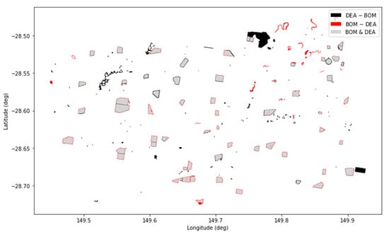
Figure 5.
Difference and intersection between DEA Waterbodies and Geofabric in the Moree test area, dominated by constructed farm storages. Differences have been smoothed and buffered by 10 m to aid visibility.
The Moree comparison shows that almost all Geofabric waterbodies are also included in DEA Waterbodies, with only minor differences along the edge of the polygon. These minor differences are due to the pixel grid of Landsat compared to the smooth and manually-curated Geofabric polygons. The Geofabric-only polygons in the northeast are rarely active and do not fulfil the >10% wet pixel threshold to be included in DEA Waterbodies. Additionally, DEA Waterbodies includes two large reservoirs that are not present in the Geofabric. The larger reservoir is often dry for entire years, and the smaller reservoir was wet only from 2016 to 2018, explaining why they were missed in the Geofabric. There is also a large creek in the northwest which the Geofabric does not include, as it manages streams separately to waterbodies. The Cranbrook comparison shows little difference in which polygons are identified, but some polygons are smaller in DEA Waterbodies than in the Geofabric (Figure A7). This is due to salt lakes being misidentified as cloud in the underlying WOfS dataset.
To perform a statistical comparison between DEA Waterbodies and the Geofabric, we associated the polygons in DEA Waterbodies and Geofabric by searching for their intersections, and assumed that intersecting polygons represented the same waterbody. If for a given polygon in one dataset there were multiple intersecting polygons in the other dataset, we assumed that all intersecting polygons were part of the same physical waterbody. We compared the areas covered by the waterbody in each dataset. The distribution of the differences in area for each waterbody is shown in Figure 6. While most waterbodies are very close in area between the two datasets (with a median deviation of 0.73% for Moree and –8.11% for Cranbrook) DEA Waterbodies and the Geofabric are much more consistent on constructed farm storages, compared to salt lakes, which tend to be smaller in DEA Waterbodies. This highlights the difficulties in defining a boundary for natural waterbodies, with DEA Waterbodies defining the polygon limit based on observed wet history, compared to Geofabric, which is manually curated.
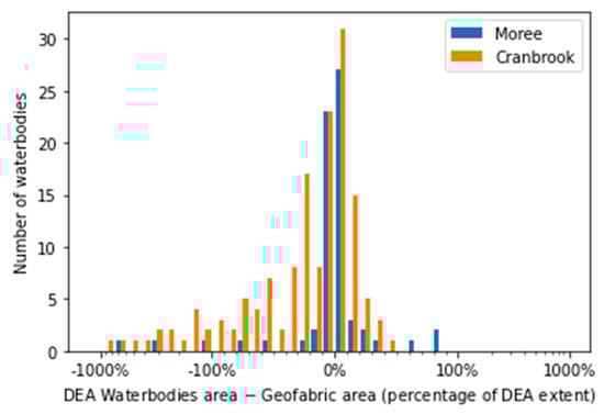
Figure 6.
Distribution of differences in area between DEA Waterbodies polygons and Geofabric polygons for the Moree and Cranbrook test areas.
We tested the asymmetric difference between all polygons in the two test areas, and computed the area of the result. This describes how much of each waterbody is contained in the Geofabric but not in DEA Waterbodies and vice versa. The distributions of these areas are shown in Figure A8. For the Cranbrook salt lakes, the difference in area is primarily due to the difference in the polygon boundary as defined in the Geofabric that is not included in DEA Waterbodies, largely due to the edges of salt lakes being masked as cloud. The Moree test site is much more symmetric, with similar rates of omission and commission between the datasets.
5.1.2. Surface Area Time Series Validation
Validation of the DEA Waterbodies time series (a wet surface area time series) is made difficult by the lack of a comparable dataset to validate against. We chose to compare a subset of DEA Waterbodies time series against gauged reservoir volume time series available through the Bureau of Meteorology’s Water Data Online (WDO) service. WDO provides volume and depth measurements for gauges in approximately 360 reservoirs, dams, and weirs around Australia. We selected a subset of 139 gauges for validation, based on the length of the gauge record, the availability and quality of depth and volume measurements, and the waterbody type (See Appendix B). We compared each volume time series to the surface area time series from DEA Waterbodies using the Spearman ρ coefficient. The Spearman coefficient measures the correlation of two datasets which have a positive monotonic relationship, regardless of whether that relationship is linear or otherwise. It can be assumed that the relationship between waterbody surface area and volume is positive monotonic, making this statistic suitable for comparison of two different measurements (surface area vs. volume), without the need to convert between them.
The locations and ρ values of the 139 gauges are shown in Figure 7. Most waterbodies show good correlation with the gauge data, with ρ coefficients > 0.8. Waterbodies in Tasmania show an overall poor relationship between DEA Waterbodies and WDO gauges. The highland lakes in Tasmania have high tannin content, making them look dark, resulting in very low levels of water leaving radiance. When combined with low solar angles this results in near-zero surface reflectance values across both the visible and near/shortwave infrared wavelengths. The normalised difference indices within the WOfS classification algorithm are extremely sensitive to noise, resulting in areas of water being misclassified as land. This causes the waterbody’s wet surface area observations to fluctuate as misclassified land pixels are counted amongst the correctly classified water pixels Figure 7d).
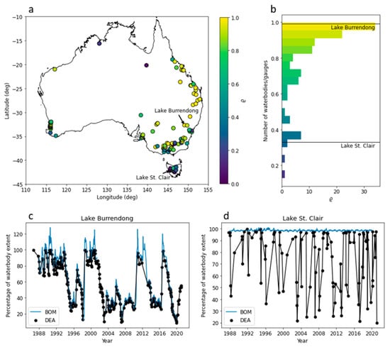
Figure 7.
Validation of DEA Waterbodies time series. (a) Spearman ρ coefficients from the DEA Waterbodies/WDO time series comparison. Waterbodies/gauges used to validate the DEA Waterbodies time series, coloured by the Spearman ρ coefficient of the relationship. (b) Distribution of Spearman ρ coefficients for all analyses. The individual gauges and their corresponding ρ are given in Appendix C, in Table A1. (c) Lake Burrendong surface area in DEA Waterbodies and estimated from WDO. (d) Lake St. Clair surface area in DEA Waterbodies and estimated from WDO. The surface areas in (c,d) are scaled as a percentage of maximum waterbody extent in DEA Waterbodies.
To help visualise the comparison between WDO and DEA Waterbodies, we estimated the surface area time series for each WDO volume time series using the volume and depth gauge data. Figure 7c and d show the estimated WDO surface area time series plotted alongside the DEA Waterbodies surface area time series for Lake Burrendong (New South Wales) and Lake St. Clair (Tasmania) respectively. The Burrendong time series (Figure 7c) shows very close agreement between the surface area time series modelled from the reservoir gauge and the surface area time series retrieved from Landsat. This is reflected in its high Spearman ρ of 0.99. The time series diverge when the dam is close to completely full. This may be due to steep slopes at the edges of the reservoir, or trees obscuring the edges of reservoir blocking the water signal and generating mixed signal pixels. The Landsat time series does not capture the 2012 filling event as this occurred in the gap between Landsat 5 and Landsat 8.
The Lake St. Clair time series (Figure 7d) shows poor agreement between the surface area time series modelled from the reservoir gauge and the surface area time series retrieved from Landsat. This is reflected in its relatively low Spearman ρ of 0.33, and is a result of a misclassification of water as land by WOfS. Based on the results of our analysis, DEA waterbodies surface area time series for Tasmanian highland lakes should be treated with caution. Such a pattern mainly occurs in the highland lakes of Tasmania, where Lake St. Clair is located. This spatial pattern is apparent in Figure 7a. In future, the WOfS water classifier will be revised to address the inaccuracies that can occur over dark waterbodies at low solar angles.
5.2. Case Studies of DEA Waterbodies Insights
DEA Waterbodies provides an unprecedented level of insights into the spatial and temporal dynamics of surface water across the Australian continent. The combination of waterbody polygons with accompanying wet area observational time series provides an opportunity to explore surface water dynamics at an individual waterbody, through to national scale. The following section presents a series of case study results that demonstrate the power of this dataset, though these do not represent an exhaustive analysis of the insights available from DEA Waterbodies.
5.2.1. Per Waterbody
Individual waterbody time series provide insights into the change in wet surface area of each waterbody across Australia, providing detailed information about the behaviour of the waterbody over time and providing indirect insights into the nature of the waterbody itself. The time series produced for each polygon corresponds well with the observed percentage of the total surface area of each waterbody observed as wet at each time step (Figure 8). These time series are most useful for indicating the timing of a change in the surface wet area, since they do not provide insights into volume. The timing of filling and emptying events is an important metric for understanding how waterbodies change over time. These changes are not attributed in DEA Waterbodies, and could result from, rainfall events, watercourse flooding, human management of a waterbody (e.g., pumping into/out of a storage), groundwater processes etc.
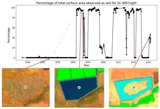
Figure 8.
Time series of the change in the percentage of total surface area observed as water for waterbody ID r6f07ug9r. The corresponding false colour imagery is shown for three time steps, showing the relationship between the time series and the raw imagery.
In constructed waterbodies (e.g., Figure 8) the wet area time series provides an indicative measure of the date the waterbody was constructed. The date that each waterbody was first observed as having at least 50% of the total waterbody area classified as wet was used as a proxy for construction date. Waterbodies that are natural and therefore not built, or waterbodies constructed prior to 1987, can be expected to return a ‘build date’ that corresponds to the first time they filled since our records began in 1987. A moderate La Niña event occurred in 1988–1989, which could be expected to fill present waterbodies across Australia’s east coast. We therefore discard any ‘build dates’ before 1990 to remove the natural and existing waterbodies from this construction analysis, but recognise that early dates may reflect water availability, rather than waterbody existence.
Prior to the construction of the storage in Figure 8, the associated time series shows almost no open water signal. Examination of satellite imagery (not shown) indicates this waterbody commenced construction in April 2000, and first began to fill with water in November 2000, registering in the time series as nearly 100% ‘wet’ for the first time in December 2000. This method can lead to bias towards very wet years, particularly in cases where waterbodies were constructed, but not filled until a wet season a few years later.
5.2.2. Per Region
Individual waterbody time series can be combined at the catchment scale to provide insights into regional-scale catchment behaviours and trends. Water management is done at multiple scales, and catchment-scale water management in Australia regularly corresponds to government policies and decisions that have been implemented at this scale [57].
The Fitzroy Basin in Queensland is one of the state’s largest basins covering an area of approximately 142,600 km2. The growth in the number of waterbodies mapped within the Fitzroy Basin reflects the development of agriculture and mining in this region (Figure 9). The recently constructed waterbodies in the northern part of the Fitzroy Basin are primarily tailings dams from mining operations [58]. Insights into the growth of waterbodies within a region provide an independent assessment of infrastructure growth, and can be used to verify the installation of approved works and potentially flag unapproved works as well. A recent paper by Malerba et al. [59] used DEA Waterbodies to explore the rate of large storage construction across Australia since 1987.
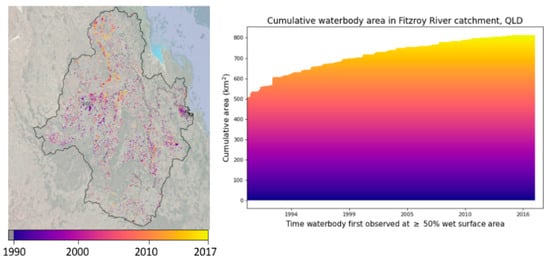
Figure 9.
Date each waterbody within the Fitzroy River Catchment, QLD, was first observed as having at least 50% of the waterbody area wet. Note that this metric indicates an approximate construction date for artificial waterbodies.
5.2.3. National/Continental
Analysis of all the waterbody time series together allows us to develop a picture of the changing nature of open surface water across Australia. The total area of waterbody polygons is 87,548.7 km2, which is approximately 1% of the total land area of Australia. The seasonal average wet area within all mapped waterbodies across Australia suggests that there is never an occasion where all mapped waterbodies contain at least some water, and there is a large degree of spatial variability in the spatial and temporal patterns of waterbody wet events (Figure 10). Two similarly extensive wet events in 1989 and 2010 show large variations in the spatial patterns of wet waterbodies across Australia. The 1989 event shows wet areas dominating in the south of the continent, corresponding with a weak La Niña event, while the 2010/11 event that coincided with a large La Niña event shows wet waterbodies mainly in eastern Australia (Figure 10). Future work will explore the spatiotemporal relationships between DEA Waterbodies and large-scale climate drivers like El Nino Southern Oscillation, Indian Ocean Dipole, and the Southern Annular Mode.

Figure 10.
National-scale seasonal wet area statistics. The bar chart at the top indicates the total wet surface area (average of all wet pixels inside waterbody polygons each year), the total dry surface area (average of all dry pixels inside waterbody polygons each year), and the total area of polygon waterbodies that was unobserved (average of all unobserved pixels inside waterbody polygons each year e.g., cloud, Landsat 7 scan-line off missing values etc.) for all waterbodies. The maps indicate the spatial pattern of the percentage of each waterbody’s surface wet area at selected time steps. The data gap in 2011/12 occurs between the Landsat 5 and Landsat 8 missions.
6. Discussion
6.1. Accuracies and Limitations of DEA Waterbodies
Accuracies and limitations of DEA Waterbodies are largely inherited from WOfS, with DEA Waterbodies a reanalysis and mapping product built off the WOfS datasets. WOfS has a number of known limitations and these manifest as incorrectly mapped waterbodies within this analysis. WOfS uses the spectral signature of water to classify wet pixels and is known to be suboptimal in locations where water and vegetation are mixed. This includes locations such as rivers with vegetated riparian zones and vegetated wetlands (Figure 11). The effect of this can be seen by the discontinuity of narrower river features identified within this analysis (Figure 11a), and by an under-representation of water within vegetated wetlands, such as the Macquarie Marshes, NSW (Figure 11b).
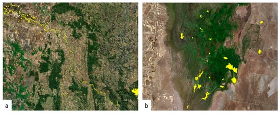
Figure 11.
Limitations of DEA Waterbodies associated with mixed water and vegetation targets. This results in (a) discontinuity within some river reaches, and (b) an under representation of waterbodies within wetlands.
Other known WOfS limitations have been addressed through the filtering processes used to produce the map of waterbodies. The size of mapped waterbodies is limited to at least five Landsat pixels, removing small, isolated ‘water’ pixels. The size filtering reduces the noise associated with the dataset by only focusing on larger groups of pixels. Misclassification of water in deep shadows in high density cities has been handled by removing any waterbody polygons identified within central business districts (CBDs). Intermittently misclassified features, which return valid results only a handful of times over the 32-year study period, are also filtered out by testing for the number of valid observations returned for each pixel.
Despite this, some errors remain in the final waterbodies dataset. Steep terrain shadows present a known difficulty for the WOfS classifier, due to the shadows produced. While WOfS has attempted to mitigate this issue, some misclassification remains. We have not specifically attempted to address these errors within this workflow, and as such, a negligible number of the identified waterbodies may in fact be artefacts caused by terrain shadow. A signal-to-noise ratio error over deeper water in the WOfS classifier has also not been addressed here, and may result in some pixels missing from the centre of deeper waterbodies, resulting in doughnut-shaped mapped polygons. Similarly, different water colours may interfere with the decision-tree classifier, resulting in very turbid or coloured waterbodies being omitted. For a full discussion of the limitations and accuracy of WOfS, see Mueller et al., 2016.
Not all waterbodies across Australia have been identified by this product, and there remain a number of known reasons why some waterbodies may have been missed:
- They might be too small: DEA Waterbodies only maps waterbodies larger than 3125 m2 (five whole Landsat pixels).
- They might not have been wet enough: DEA Waterbodies only maps waterbodies that have been observed as wet at least 10% of the time between 1987 and 2018. If a waterbody fills very infrequently, it may not meet this threshold.
- The waterbodies might have too much vegetation surrounding them: The WOfS classifier does not work well where water is combined with vegetation. If there is vegetation obscuring the water (like a tree leaning across a river, or a wetland), the classifier will not see this as water and the waterbody may not be mapped.
- The waters in the waterbodies are not classified as water: Sediment rich water or other unusual water spectra [60], like those in algae-rich waterbodies can confuse the WOfS classifier, resulting in the pixels being incorrectly classified as not water.
- The waterbodies might be new: Waterbodies that have been constructed or modified after 2016 may not be captured within this tool as they will not have been observed as wet at least 10% of the time between 1987 and 2018. Future updates of this product should capture newer waterbodies.
The automated nature of DEA Waterbodies identification and mapping means that some artefacts exist in the waterbody outlines, which do not directly match the real-world waterbody shape. Waterbodies have been mapped by DEA Waterbodies using the resolution of Landsat, so the outlines of every waterbody are pixelated, and may not be an exact representation of the real-world shape of the waterbody. Since DEA Waterbodies uses an automatic workflow utilising Landsat data to objectively map waterbodies, we have chosen to leave the final waterbody line work pixelated to transparently identify which Landsat pixels have been mapped inside (and outside) of each waterbody (Figure 12). Future iterations of DEA Waterbodies could make use of sub-pixel methods [25,26,27,28] or higher resolution imagery to better capture the true waterbody shape.
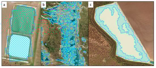
Figure 12.
Known limitations with the DEA Waterbodies outlines. (a) multiple waterbodies mapped as a single waterbody; (b) complex waterbody boundaries resulting in many small polygons rather than a single large polygon; (c) incomplete waterbody outlines.
The relatively coarse spatial resolution of Landsat and WOfS has resulted in the loss of some discontinuities like dam walls, causing multiple waterbodies to be mapped as a single polygon (Figure 12a). This is most common where separating features like dam walls or banks are relatively narrow, resulting in mixed water/land pixels being recorded over these features, and losing the clear distinction between two waterbodies within the Landsat data. Conversely, discontinuities in the water classifier caused by real world features such as small discrete water pools, or spatial variability in the frequency of inundation within a single waterbody, or limitations in the WOfS classifier as described above, have resulted in waterbodies being mapped as a large number of small polygons, rather than a single connected waterbody (Figure 12b), or the extent of the waterbody being incompletely captured by the polygon (Figure 12c).
The production of DEA Waterbodies using an objective, coded workflow means that as new data become available, the workflow can be easily re-run to update the analysis and improve the overall dataset quality. Future work that makes use of Sentinel 2 data will increase the spatial and temporal resolution of the analysis, and assist in developing a more accurate DEA Waterbodies map. Discontinuities caused by real world features could be minimised in future data releases by removing holes from ‘doughnut-shaped’ polygons, however this would require additional work to explore how much this process would help improve the quality of the DEA Waterbodies map, rather than introduce new sources of error.
Identified waterbodies are a combination of natural and man-made waterbodies, and contain features such as rivers, lakes, water supply dams, on farm storages, wetlands, oxbow lakes, and ponds. The DEA Waterbodies product does not identify the nature of the waterbody (natural vs. man-made) nor its purpose. We also do not attempt to label features that have a known name and instead use the geohash as a unique identifier. This means that well known features such as Kati Thanda–Lake Eyre are not labelled with their common name in this product, and are instead referred to just using their geohash (e.g., r4ctk0hzm). DEA Waterbodies could be spatially joined with the Geofabric [61] to attach names from previously mapped features, however differences in the extents of mapped features between these two products may make this task difficult.
6.2. Comparison of DEA Waterbodies against Other Datasets
National-scale water mapping has been done previously over all of Australia, however DEA Waterbodies represents the first, national-scale, satellite-derived polygon dataset of waterbodies across the continent. Pekel et al., 2016 and Pickens et al., 2020 both present global surface water maps, comparable to WOfS. Both of these products look at the frequency of water for each individual pixel, but do not provide vector-based analyses of surface water, making it more difficult to interrogate whole waterbodies. Pekel et al., 2016 and Pickens et al., 2020 provide the ability to generate a time series of water history for each individual pixel, adding some time context to the water maps. While this functionality is similar to DEA Waterbodies, our ability to track the surface area of water over time across a whole waterbody provides insights into the behaviour of the waterbody as a whole, rather than an arbitrary pixel within it.
The Blue Dot Water Observatory (https://www.blue-dot-observatory.com/; [62] accessed on 31 March 2021) provides insights into the change in surface area of water, much like DEA Waterbodies, however on a much more limited spatial and temporal scale. The Blue Dot Observatory allows users to interrogate changes in the surface area of water for 188 identified waterbodies across Australia (40,330 globally) using the archive of Sentinel 2 data. The period of common data coverage between DEA Waterbodies and The Blue Dot Observatory shows a high degree of similarity between the results derived from the two products. This acts as an additional validation of our methods, which source different waterbody extent polygons, use different water detection algorithms and use different satellites to produce the outputs. The use of Landsat to derive the waterbody extents and time series histories in DEA Waterbodies extends the length of the analysis back to 1987, compared to Blue Dot Water Observatory’s five-year record from Sentinel 2.
6.3. DEA Waterbodies Applied Case Study
The development of a satellite-based waterbody map for all of Australia means that regional and national-scale monitoring of the state of Australia’s surface waterbodies can be carried out routinely. DEA Waterbodies is being used in the New South Wales (NSW) Department of Primary Industries Monthly Seasonal Conditions State Seasonal Update [63]. The State Seasonal Update is a monthly report containing an overview of the current climate and drought state of NSW provided to government, industry, landholders and the public. Data from DEA Waterbodies are resampled to a parish scale (to de-identify the data) and mapped according to the average wet surface area within all storages in that parish. This update provides an indication of stock water availability, as well as the potential risk to agricultural water supply in the region. Insights gained from the State Seasonal Update are being used by government to help inform drought mitigation strategies and financial support [64].
7. Conclusions
DEA Waterbodies maps and monitors almost 300,000 waterbodies across Australia, providing updating insights into the change in the wet surface area within each waterbody over time. DEA Waterbodies also provides insights into the behaviour of individual waterbodies over time, and can be used to gain insights into drought, regional-scale development, water management practices, and water spatial variability. Future versions of this product will make use of the higher temporal and spatial resolution of Sentinel 2 satellites to improve both the quality of the waterbody polygons themselves, and the frequency with which they are observed. The provision of both the code used to develop DEA Waterbodies and the outputs datasets under open-source licenses will facilitate future work in this area, allowing others to build off the results presented here.
While DEA Waterbodies provides new insights into the change in surface water area within waterbodies over time, water managers need to understand changes in water volume to input into water balance accounts. Future work will integrate DEA Waterbodies with LiDAR data to derive surface area/volume curves for individual waterbodies, allowing an uncertainty-bounded estimate of volume changes to be provided alongside changes in wet surface area. This will make the product much more useful to water managers and the water industry, who need to monitor and understand the movement of water volumes within a catchment over time.
National-scale reporting on water availability is a critical metric for the United Nation Sustainable Development Goal (SDG) six: clean water and sanitation. DEA Waterbodies provides a mechanism for reporting against SDGs by providing snapshots in time of the amount and spatial locations of surface water across Australia. Development of the product to include volume estimates will also increase the relevance of DEA Waterbodies to this type of national-scale reporting.
Author Contributions
Conceptualization, C.E.K. and L.L.; methodology, C.E.K.; software, C.E.K., V.N. and M.J.A.; validation, C.E.K., V.N. and M.J.A.; investigation, C.E.K. and V.N.; writing—original draft preparation, C.E.K. and L.L.; writing—review and editing, C.E.K., L.L., M.J.A. and V.N. All authors have read and agreed to the published version of the manuscript.
Funding
This research was supported by a grant from the New South Wales Department of Primary Industries (now NSW Department of Planning, Industry and Environment).
Data Availability Statement
The data presented in this study are openly available. DEA Waterbodies polygons can be downloaded from http://pid.geoscience.gov.au/dataset/ga/132814 (accessed on 31 March 2021). Wet surface area time series can be accessed via https://maps.dea.ga.gov.au/ (accessed on 31 March 2021). The code used to produce DEA Waterbodies is open source, provided under an Apache Licence, Version 2.0, and can be found at https://github.com/GeoscienceAustralia/dea-waterbodies (accessed on 31 March 2021). Additional documentation on the access and use of DEA Waterbodies is available at https://www.ga.gov.au/dea/products/dea-waterbodies (accessed on 31 March 2021).
Acknowledgments
This research was undertaken with the assistance of resources from the National Computational Infrastructure (NCI Australia), an NCRIS enabled capability supported by the Australian Government. This paper is published with the permission of the CEO, Geoscience Australia.
Conflicts of Interest
The authors declare no conflict of interest.
Appendix A
Details of the methodology used to produce DEA Waterbodies is provided here to facilitate reproducibility of the workflow. The code produced for this workflow can be found here: https://github.com/GeoscienceAustralia/dea-waterbodies (accessed on 31 March 2021), and is open source, provided under an Apache Licence, Version 2.0.
Appendix A.1. Step 1: Check Each Pixel Has Been Observed ≥128 Times
The maximum extent of each waterbody is identified using WOfS classified scenes from Landsat from 1987 to 2018. The number of valid WOfS observations for each pixel varies depending on the frequency of clouds and cloud shadow, the proximity to high slope and terrain shadow, and the seasonal change in solar angle. The ‘count_clear’ parameter, calculated within the WOfS all time summaries, provides a count of the number of valid observations each pixel recorded over the analysis period. We can use this parameter to mask out pixels that were infrequently observed. If this mask is not applied, pixels that were observed only once could be included, if that observation was wet (i.e., a single wet observation means the calculation of the frequency statistic would be (1 wet observation)/(1 total observation) = 100% frequency of wet observations). A threshold for the number of clear, valid observations needed to be determined to generate a filter to exclude pixels that were not observed frequently enough over the 32-year analysis period. We chose to set this threshold at 128 valid observations, equating to roughly four observations per year, though we do not require that the timing of valid observations meets any temporal regularity.
Appendix A.2. Step 2: Check Each Pixel Meets 5% and/or 10% Wet Frequency Threshold
The WOfS Statistics was filtered to remove pixels that were infrequently wet, as we wanted to define waterbodies where water persists in the landscape, rather than floodplains. The threshold used to filter out low frequency wet pixels can be varied based on the required sensitivity of the output to flood events. Similarly, this threshold could be set higher to identify the locations of refugial waterbodies.
For this analysis, a sensitivity test was conducted to determine the effect of different wet frequency thresholds on the number and size of resulting waterbody polygons. The wet frequency threshold indicates how frequently a pixel needed to be observed as wet in order to be included. A wet frequency threshold of 0.1 means that at least 10% of the total, valid observations needed to be classified as ‘wet’. Five wet frequency thresholds were tested: 0.01, 0.02, 0.05, 0.1 and 0.2. The suitability of each threshold was tested in three separate locations, representing three different landcover types: desert floodplain, irrigated cropping, combination of natural water and irrigated cropping.

Figure A1.
Wet frequency threshold impacts on (a) the total number of individual mapped waterbodies, (b) the total area contained within the individual mapped waterbodies. Individual scatter points represent integrations over different time periods from 1987 to 2018.
Figure A1.
Wet frequency threshold impacts on (a) the total number of individual mapped waterbodies, (b) the total area contained within the individual mapped waterbodies. Individual scatter points represent integrations over different time periods from 1987 to 2018.

The influence of the varying wet frequency thresholds on both the number and area of identified waterbodies was explored (Figure A1). The lower the wet frequency threshold applied, the larger both the number of total identified polygons, and the area of individual polygons (Figure A1). The area distribution of identified polygons is consistent between wet frequency thresholds, with the absolute number of polygons the changing parameter (Figure A1a). The number and areas of polygons identified by the 0.1 and 0.05 thresholds are relatively consistent, suggesting that these wet frequency thresholds result in similar numbers and size distributions of waterbody polygons. The changing sensitivity of the wet frequency threshold on the total area of waterbodies identified (Figure A1b), shows an exponential relationship, highlighting the importance of finding the balance between errors of omission and commission.
While an objective analysis of the suitability of different wet frequency thresholds is preferred, the final decision on the wet frequency thresholds used was determined based on looking at the suitability of the individual waterbody polygons identified by each threshold. The outputs in Figure A2 demonstrate the impact of the wet frequency thresholds on waterbody polygon locations and shapes, however the thresholding is applied at the pixel level prior to turning adjoining pixels into polygons. The lowest two thresholds (0.01 and 0.02), return a lot of noisy pixels that contain some striping from Landsat 7’s scan line corrector failure, as well as a lot of small polygons that do not clearly line up with waterbody features (Figure A2a). At the other end of the sensitivity thresholds, 0.2 was shown to be not sensitive enough, missing both the maximum extent of some identified features, or missing whole waterbodies entirely (Figure A2b).

Figure A2.
Waterbody polygons identified using the different wet frequency thresholds. The color of the polygon indicates the highest threshold that an area is identified by, e.g., if you see an area in pink, this has been detected by the 0.05, 0.02 and 0.01 thresholds; if it’s blue, then it has been detected by all thresholds etc. (a) All wet frequency threshold polygons. (b) 0.01 (yellow) and 0.02 (green) thresholds removed. Locations missed by the 0.2 (blue) threshold are shown in pink/orange. (c) Just 0.05 (pink) and 0.1 (orange) thresholds. Locations missed by the 0.1 (orange) threshold are shown in pink. (d) Just 0.05 (pink) and 0.1 (orange) thresholds. Locations missed by the 0.1 (orange) threshold are shown in pink. Legend for all figures as in (a).

Both the 0.05 and 0.1 thresholds showed both errors of omission and commission, depending on the location in which they were applied. In a location with large areas of flood irrigation, the 0.05 threshold identified a number of paddocks as waterbodies, indicating this threshold is too sensitive in these conditions (Figure A2c). In more arid areas, where waterbodies rarely reach their maximum extent, the 0.1 threshold was shown to underrepresent the maximum waterbody extent, picking out only partial polygons within individual waterbodies (Figure A2d). Given the limitations of both wet frequency thresholds, a hybrid threshold was chosen, whereby the locations of waterbodies were identified using the 0.1 threshold, but the spatial extent of these waterbodies was characterised using the 0.05 threshold. This minimises commissions caused by flood irrigation, which are not readily captured by the 0.1 wet frequency threshold, but also captures the larger spatial extent of individual waterbodies afforded by the 0.05 threshold. While we have chosen a 0.1/0.05 threshold for our purposes, the workflow has been written to allow the user to define their own single, or hybrid threshold, making it customisable to different environmental conditions.
Appendix A.3. Step 3: Turn Wet Pixels into Polygons
In order to treat pixels from common waterbodies in the same way, we polygonise the raster to produce polygons that represent the outlines of wet waterbodies. Once the wet frequency threshold had been applied to the data, pixels that did not meet this threshold were set to ‘NaN’ and pixels that were to be included were set to ‘1’. This was done to ensure that the boundaries of each waterbody were easily discernable prior to converting them into polygons, to minimise errors caused by the polygonisation process (Figure A3).

Figure A3.
Polygonisation process to transfer pixels identified as waterbodies (a) into polygons (b).
Figure A3.
Polygonisation process to transfer pixels identified as waterbodies (a) into polygons (b).

Appendix A.4. Step 4: Merge Polygons Artificially Cut by Tile Boundaries
The workflow has been designed to be completed on individual Albers Equal Areas tiles across Australia as a means to break up the processing into sensible chunks. A temporary shapefile was written that included all of the identified polygons for each individual tile. This shapefile was appended to following each tile’s processing. This resulted in waterbodies that straddle tile boundaries being segmented artificially at the tile boundary. To correct this, we created a one-pixel buffer around the Albers Equal Area tile grid, identified any polygons that intersected with this buffer, and merged any selected polygons that touched.
Appendix A.5. Step 5: Filter Polygons by Max and Min Size
A size filter was applied to the mapped waterbody polygons that removed polygons below five Landsat 25 m by 25 m pixels in size (3125 m2). This threshold was set to limit noise associated with very small waterbodies. As a result of this threshold, small farm storages and small sections of river have also been excluded from the final product.
The workflow has been designed to allow the user to specify their own size thresholds, which can be modified depending on the desired outcome.
Appendix A.6. Step 6: Remove Polygons Containing Ocean
A coastline dataset is used to remove waterbodies containing ocean. The user can choose which coastline dataset to use, depending on whether they would like features like estuaries included in the final product. Here, we use a coastline based on the Intertidal Extents Model version 2 (ITEM [65]), which uses Landsat data to generate snapshots of the Australian coastline at different tidal heights. We use the highest tide modelled by ITEM (pixels exposed at highest 80–100% of the observed tidal range (land) [66]) to represent the high-tide coastline of Australia. In order to remove estuaries and some inland lakes, we considered any pixel connected to the ocean to be ‘ocean’, and were thus removed by this mask. The mask has a number of limitations, which result in parts of tidal river estuaries being mapped as waterbodies. These primarily occur where there is a discontinuity in the water signal along the river channel, caused by large bridges or narrowing river channels, for example (Figure A4).

Figure A4.
Ocean mask used to remove ocean and ocean-connected waterbodies from the final product. The mask incorrectly fails to map some complete estuaries where the water signal from the ocean is not continuous, like seen above in Perth, Western Australia, where two large bridges have terminated the ocean mask prematurely (yellow squares).

Appendix A.7. Step 7: Remove Polygons within CBDs
The WOfS dataset has a known limitation, whereby deep shadows caused by high rise buildings in CBDs are classified as water [19]. This means that our workflow is defining ‘waterbodies’ around these misclassified shadows in capital cities (Figure A5). To address this problem, we use the Australian Bureau of Statistics Statistical Area 3 (SA3) shapefile [67] to define a spatial footprint for Australia’s CBD areas. The SA3 boundaries are a regional population grouping that contain between 30,000 and 130,000 people, typically clustered around commercial and transport hubs [68].
We use the following SA3 statistical areas as our CBD filter: 11703: Sydney Inner City, 20604: Melbourne City, 30501: Brisbane Inner, 30901: Broadbeach–Burleigh, 30910: Surfers Paradise, 40101: Adelaide City, 50302, Perth City. The CBDs of other cities, such as Canberra and Darwin, do not contain enough high-rise buildings to be affected, and so were not used within this filter.

Figure A5.
Incorrectly identified waterbodies within the Sydney CBD.
Figure A5.
Incorrectly identified waterbodies within the Sydney CBD.

Appendix A.8. Step 8: Find Polygons within the 5% Wet Frequency Threshold Layer That Intersect with the 10% Wet Frequency Threshold Layer
The hybrid wet frequency threshold discussed above is applied in this step. Up until this point, two parallel analyses are being run—the 5% wet frequency threshold and the 10% wet frequency threshold. The filtering steps described in the workflow up until this point are applied independently to these two differently thresholded products, producing two outputs. At this point, we perform a spatial join on the two polygon datasets to find locations where the 10% and 5% threshold overlap. Where a polygon in the 10% wet frequency output is found to overlap with the 5% wet frequency product, the polygon from the 5% wet frequency product is kept, and the 10% wet frequency polygon is thrown away. This means that the locations of the waterbody polygons are defined by the 10% wet frequency threshold, but the extent of the polygon is defined by the 5% wet frequency threshold. This produces more spatially extensive polygons, but only in locations that have been identified with the more conservative threshold.
Appendix A.9. Step 9: Use the Polsby-Popper Test to Identify and Split Very Large Polygons
The final waterbodies shapefile was checked for large river segments using the Polsby–Popper statistical test [53]. The Polsby–Popper test is an assessment of the ‘compactness’ of a polygon. This method was originally developed to test the shape of congressional and state legislative districts, to prevent gerrymandering. The Polsby–Popper test examines the ratio between the area of a polygon, and the area of a circle equal to the perimeter of that polygon. The result falls between 0 and 1, with values closer to 1 being assessed as more compact. We selected all polygons with a Polsby–Popper test value ≤ 0.005 for further interrogation. This resulted in a subset of 186 polygons (Figure A6).
The 186 polygons were buffered with a −50 m (2 pixel) buffer to separate the polygons where they are connected by two pixels or less. This allows us to split up these very large polygons by using natural thinning points. The resulting negatively buffered polygons was run through the multipart to singlepart tool in QGIS, to give the now separated polygons unique IDs. These polygons were then buffered with a +50 m buffer to return the polygons to approximately their original size. These final polygons were used to separate the 186 original polygons identified above.

Figure A6.
Initial DEA Waterbodies product, with polygons with a Polsby-Popper test value ≤ 0.005 highlighted in red.
Figure A6.
Initial DEA Waterbodies product, with polygons with a Polsby-Popper test value ≤ 0.005 highlighted in red.

The process for dividing up the identified very large polygons varied depending on the polygon in question. Where large waterbodies (like the Menindee Lakes) were connected, the buffered polygons were used to determine the cut points in the original polygons. Where additional breaks were required, the Bureau of Meteorology’s Geofabric v3.0.5 Beta [61] waterbodies dataset was used as an additional source of information for breaking up connected segments.
The buffering method didn’t work on long segments of river, which became a series of disconnected pieces when negatively and positively buffered. Instead, we used a combination of tributaries and man-made features such as bridges and weirs to segment these river sections. Where no tributaries existed, large river segments were split using the Albers Equal Area tile boundaries.
This method was used to produce an objective flag for waterbodies that may need to be split to produce smaller and more meaningful waterbody polygons as well as a semi-objective means for splitting large polygons. As much as was possible, decisions were hard coded to make them repeatable for future runs of this workflow.
Appendix A.10. Step 10: Generate a Geohash ID for Each Polygon
A unique identifier is required for every polygon to allow it to be referenced. The naming convention for generating unique IDs here is the Geohash [69]. A Geohash is a geocoding system used to generate short unique identifiers based on latitude/longitude coordinates. It is a short combination of letters and numbers, with the length of the string a function of the precision of the location. We use the python package ‘python-geohash’ to generate a Geohash unique identifier for each polygon. We use precision = 9 geohash characters, which represents an on the ground accuracy of <20 m. This ensures that the precision is high enough to differentiate between waterbodies located next to each other. Finally, individual polygon areas were recalculated and added as an attribute to the final waterbody shapefile.
Appendix B. Geofabric Polygon Comparison
This appendix shows the spatial differences between DEA Waterbodies and Geofabric. Figure A7 shows the Moree test area, which mostly contains farm dams, and Figure A8 shows the Cranbrook test area, which is dominated by salt lakes. The difference polygons have been smoothed and buffered by 10 m to aid visibility.

Figure A7.
Difference and intersection between DEA Waterbodies and Geofabric in the Cranbrook test area.
Figure A7.
Difference and intersection between DEA Waterbodies and Geofabric in the Cranbrook test area.


Figure A8.
Distribution of areas of the difference polygons between DEA Waterbodies polygons and Geofabric polygons for the Moree and Cranbrook test areas.
Figure A8.
Distribution of areas of the difference polygons between DEA Waterbodies polygons and Geofabric polygons for the Moree and Cranbrook test areas.

Appendix C. Water Data Online Time Series Comparison
This appendix details the water level and volume gauges used to validate DEA Waterbodies and the corresponding Spearman ρ values of the comparison.
The Water Data Online service maintained by the Bureau of Meteorology provides volume and depth measurements for gauges in approximately 360 reservoirs, dams, and weirs around Australia. We selected a subset of these gauges for validation based on the following criteria:
- The gauge needed to have at least 10 years of data.
- Depth and volume measurements needed to be related, i.e., an increase in depth needed to be associated with an increase in volume.
- Gauges at weirs and locks were removed, since a gauged volume at a weir is not comparable to a waterbody polygon, and they cannot be meaningfully compared.
- Exceptionally noisy gauge time series were removed. This was determined by manual inspection of each time series. Gauges were removed where there were erroneous spikes in data, prolonged data gaps and values that didn’t change over time, where they could be expected to.
- Gauges that did not correspond to a polygon of a waterbody in DEA Waterbodies were removed.
Thus, 139 volume gauges remained, and were compared against the corresponding DEA Waterbodies polygon time series using the Spearman coefficient (ρ). These correlations are shown in Table A1.

Table A1.
Storage gauges and the ρ values from comparing their time series to DEA Waterbodies.
Table A1.
Storage gauges and the ρ values from comparing their time series to DEA Waterbodies.
| Gauge | ρ |
|---|---|
| Arthurs Lake—At Pump Station | 0.889 |
| Aroona Creek/Dam | 0.845 |
| Brogo Dam | 0.506 |
| Bronte Lagoon—At Dam | 0.713 |
| Burbury Lake—At Crotty Dam | 0.442 |
| Burrendong Dam | 0.991 |
| Barkers Creek Storage | 0.955 |
| Bjelke-Petersen Dam | 0.989 |
| Boondooma Dam | 0.986 |
| Burdekin Falls Dam | 0.948 |
| Cargelligo Storage | 0.950 |
| Cluny Lagoon—At Dam | 0.358 |
| Cairn Curran Reservoir | 0.993 |
| Callide Dam (Intake) | 0.997 |
| Canning Wsl—Logger Data | 0.934 |
| Canning Wsl-Ranger | 0.934 |
| Cascade Ck Dam No. 2 | 0.364 |
| Churchman Bk Wsl-Ranger | 0.900 |
| Clarendon Head Water | 0.973 |
| Coolmunda Dam | 0.990 |
| Corin Res. At Dam | 0.860 |
| Cotter Res. At Dam | 0.723 |
| Devilbend Reservoir | 0.787 |
| Dartmouth | 0.913 |
| Drakes Bk Wsl | 0.729 |
| Echo Lake—At Dam | 0.665 |
| Eildon | 0.989 |
| Eungella Dam | 0.923 |
| Fellmongers C At Res | 0.887 |
| Fairbairn Dam | 0.992 |
| Fred Haigh Dam | 0.974 |
| Great Lake—At Poatina Inlet | 0.737 |
| Greaves Creek Dam | 0.849 |
| Geehi At Geehi Res | 0.326 |
| Glen Mervyn Wsl—Logger | 0.907 |
| Googong Res At Dam | 0.855 |
| Greens Lake | 0.968 |
| Guthega Pondage Rl | 0.437 |
| Happy Valley Reservoir (Sa Water) | 0.702 |
| Harding Dam Water Levels—Site Readings | 0.953 |
| Harris Wsl | 0.846 |
| Harvey Dam Water Level | 0.974 |
| Harvey Dam Water Level-Logger | 0.970 |
| Harvey Dam Water Level-Manual | 0.975 |
| Jounama Pondage Rl | 0.854 |
| Julius Dam Hw | 0.661 |
| Keepit Dam | 0.998 |
| Kangaroo Creek Reservoir (Sa Water) | 0.959 |
| Kerferd Reservoir | 0.720 |
| Kinchant Dam Hw | 0.864 |
| Kroombit Dam | 0.946 |
| L Pamararoo Copi H | 0.943 |
| L Wetherell Tandure | 0.962 |
| Lake Cawndilla | 0.982 |
| Lal Lal Res. H.G. | 0.901 |
| Laughing Jack Lagoon—At Dam | 0.879 |
| Lake Awoonga | 0.817 |
| Lake Eucumbene Rl | 0.955 |
| Lake Mokoan | 0.991 |
| Lake Nillahcootie | 0.954 |
| Lake Paluma | 0.666 |
| Lake Victoria Wl | 0.884 |
| Leslie Dam | 0.993 |
| Little Para Reservoir (Sa Water) | 0.944 |
| Logue Brook Wsl | 0.986 |
| Loombah Reservoir | 0.369 |
| Mackenzie Lake—At Dam | 0.809 |
| Mackintosh Lake—At Dam | 0.470 |
| Margaret Lake—At Dam | 0.128 |
| Moorabool Wb Res Hg | 0.960 |
| Malmsbury Reservoir | 0.988 |
| Mccay Storage | 0.687 |
| Millbrook Reservoir (Sa Water) | 0.880 |
| Moochalabra WSL | 0.825 |
| Moochalabra Wsl Logged Dow | 0.574 |
| Mt Bold Reservoir (Sa Water) | 0.957 |
| Mundaring Wsl-Logger | 0.930 |
| Mundaring Wsl-Ranger | 0.911 |
| Myponga Reservoir (Sa Water) | 0.931 |
| New Victoria Water Level-Ranger | 0.930 |
| Nil Gully Reservoir | 0.351 |
| North Pine | 0.935 |
| Nth Dandalup Wsl—Logger Data | 0.968 |
| Pine Tier Lagoon—At Dam | 0.692 |
| Paradise Dam | 0.925 |
| Peter Faust Dam | 0.950 |
| Prospect Reservoir | 0.664 |
| Quickup Wsl—Logger | 0.768 |
| Rocklands Reservoir | 0.986 |
| Ross Dam | 0.961 |
| Silvan Reservoir | 0.360 |
| Scabby Gully Dam Wsl Logger | 0.622 |
| Serpentine Main Dam Wsl—Ranger | 0.954 |
| South Para Reservoir (Sa Water) | 0.940 |
| St.Clair Lake—at Pump House Point | 0.330 |
| Sth Dandalup Wsl-Ranger | 0.968 |
| Stirling Wsl—Logger Data | 0.856 |
| Thomson Reservoir | 0.957 |
| Trevallyn Lake—At Dam | 0.389 |
| Talbingo Res—Ro | 0.224 |
| Tantangara Dam Rl | 0.985 |
| Teemburra Dam | 0.712 |
| Upper Coliban Reservoir | 0.944 |
| Upper Stony Creek No. 2 | 0.601 |
| Upper Stony Creek No. 3 | 0.876 |
| Upper Stony Creek Reservoirs | 0.362 |
| Waranga Basin | 0.987 |
| Watts Riv-Maroondah | 0.868 |
| Wayatinah Lagoon—At Intake | 0.621 |
| Windamere Dam | 0.962 |
| Woods Lake—At Dam | 0.776 |
| Woronora R. @ Dam | 0.824 |
| Waroona Dam Water Level Logger | 0.842 |
| Warragamba | 0.907 |
| Wartook Reservoir | 0.752 |
| White Swan | 0.928 |
| Wurdee Boluc Reservoir | 0.855 |
| Yarra Riv-Uy Res Hg | 0.927 |
References
- Bakker, K. Water Security: Research Challenges and Opportunities. Science 2012, 337, 914–915. [Google Scholar] [CrossRef]
- Grill, G.; Lehner, B.; Thieme, M.; Geenen, B.; Tickner, D.; Antonelli, F.; Babu, S.; Borrelli, P.; Cheng, L.; Crochetiere, H.; et al. Mapping the World’s Free-Flowing Rivers. Nature 2019, 569, 215–221. [Google Scholar] [CrossRef]
- Haddeland, I.; Heinke, J.; Biemans, H.; Eisner, S.; Flörke, M.; Hanasaki, N.; Konzmann, M.; Ludwig, F.; Masaki, Y.; Schewe, J.; et al. Global Water Resources Affected by Human Interventions and Climate Change. Proc. Natl. Acad. Sci. USA 2014, 111, 3251–3256. [Google Scholar] [CrossRef]
- Vörösmarty, C.J.; McIntyre, P.B.; Gessner, M.O.; Dudgeon, D.; Prusevich, A.; Green, P.; Glidden, S.; Bunn, S.E.; Sullivan, C.A.; Liermann, C.R.; et al. Global Threats to Human Water Security and River Biodiversity. Nature 2010, 467, 555–561. [Google Scholar] [CrossRef]
- Vörösmarty, C.J.; Green, P.; Salisbury, J.; Lammers, R.B. Global Water Resources: Vulnerability from Climate Change and Population Growth. Science 2000, 289, 284–288. [Google Scholar] [CrossRef] [PubMed]
- Gleick, P.H. Water and Terrorism. Water Policy 2006, 8, 481–503. [Google Scholar] [CrossRef]
- Rodell, M.; Famiglietti, J.S.; Wiese, D.N.; Reager, J.T.; Beaudoing, H.K.; Landerer, F.W.; Lo, M.-H. Emerging Trends in Global Freshwater Availability. Nature 2018, 557, 651–659. [Google Scholar] [CrossRef] [PubMed]
- Wouters, P. Water Security: Global, Regional and Local Challenges; Institute for Public Policy Research: London, UK, 2010; p. 17. [Google Scholar]
- Hou, J.; van Dijk, A.I.J.M.; Beck, H.E. Global Satellite-Based River Gauging and the Influence of River Morphology on Its Application. Remote Sens. Environ. 2020, 239, 111629. [Google Scholar] [CrossRef]
- Sheffield, J.; Wood, E.F.; Pan, M.; Beck, H.; Coccia, G.; Serrat-Capdevila, A.; Verbist, K. Satellite Remote Sensing for Water Resources Management: Potential for Supporting Sustainable Development in Data-Poor Regions. Water Resour. Res. 2018, 54, 9724–9758. [Google Scholar] [CrossRef]
- Uereyen, S.; Kuenzer, C.A. Review of Earth Observation-Based Analyses for Major River Basins. Remote Sens. 2019, 11, 2951. [Google Scholar] [CrossRef]
- Pekel, J.-F.; Cottam, A.; Gorelick, N.; Belward, A.S. High-Resolution Mapping of Global Surface Water and Its Long-Term Changes. Nature 2016, 540, 418–422. [Google Scholar] [CrossRef]
- Pickens, A.H.; Hansen, M.C.; Hancher, M.; Stehman, S.V.; Tyukavina, A.; Potapov, P.; Marroquin, B.; Sherani, Z. Mapping and Sampling to Characterize Global Inland Water Dynamics from 1999 to 2018 with Full Landsat Time-Series. Remote Sens. Environ. 2020, 243, 111792. [Google Scholar] [CrossRef]
- Wulder, M.A.; Masek, J.G.; Cohen, W.B.; Loveland, T.R.; Woodcock, C.E. Opening the Archive: How Free Data Has Enabled the Science and Monitoring Promise of Landsat. Remote Sens. Environ. 2012, 122, 2–10. [Google Scholar] [CrossRef]
- Wulder, M.A.; White, J.C.; Loveland, T.R.; Woodcock, C.E.; Belward, A.S.; Cohen, W.B.; Fosnight, E.A.; Shaw, J.; Masek, J.G.; Roy, D.P. The Global Landsat Archive: Status, Consolidation, and Direction. Remote Sens. Environ. 2016, 185, 271–283. [Google Scholar] [CrossRef]
- Woodcock, C.E.; Allen, R.; Anderson, M.; Belward, A.; Bindschadler, R.; Cohen, W.; Gao, F.; Goward, S.N.; Helder, D.; Helmer, E.; et al. Free Access to Landsat Imagery. Science 2008, 320, 1011. [Google Scholar] [CrossRef] [PubMed]
- Khandelwal, A.; Karpatne, A.; Marlier, M.E.; Kim, J.; Lettenmaier, D.P.; Kumar, V. An Approach for Global Monitoring of Surface Water Extent Variations in Reservoirs Using MODIS Data. Remote Sens. Environ. 2017, 202, 113–128. [Google Scholar] [CrossRef]
- Yamazaki, D.; Trigg, M.A.; Ikeshima, D. Development of a Global ~90m Water Body Map Using Multi-Temporal Landsat Images. Remote Sens. Environ. 2015, 171, 337–351. [Google Scholar] [CrossRef]
- Mueller, N.; Lewis, A.; Roberts, D.; Ring, S.; Melrose, R.; Sixsmith, J.; Lymburner, L.; McIntyre, A.; Tan, P.; Curnow, S.; et al. Water Observations from Space: Mapping Surface Water from 25 Years of Landsat Imagery across Australia. Remote Sens. Environ. 2016, 174, 341–352. [Google Scholar] [CrossRef]
- Tulbure, M.G.; Broich, M.; Stehman, S.V.; Kommareddy, A. Surface Water Extent Dynamics from Three Decades of Seasonally Continuous Landsat Time Series at Subcontinental Scale in a Semi-Arid Region. Remote Sens. Environ. 2016, 178, 142–157. [Google Scholar] [CrossRef]
- Tulbure, M.G.; Broich, M. Spatiotemporal Dynamic of Surface Water Bodies Using Landsat Time-Series Data from 1999 to 2011. ISPRS J. Photogramm. Remote Sens. 2013, 79, 44–52. [Google Scholar] [CrossRef]
- Xu, N.; Ma, Y.; Zhang, W.; Wang, X.H. Surface-Water-Level Changes during 2003-2019 in Australia Revealed by ICESat/ICESat-2 Altimetry and Landsat Imagery. IEEE Geosci. Remote Sens. Lett. 2020, 1–5. Available online: https://ieeexplore.ieee.org/document/9104913 (accessed on 24 November 2020). [CrossRef]
- Feng, M.; Sexton, J.O.; Channan, S.; Townshend, J.R. A Global, High-Resolution (30-m) Inland Water Body Dataset for 2000: First Results of a Topographic–Spectral Classification Algorithm. Int. J. Digit. Earth 2016, 9, 113–133. [Google Scholar] [CrossRef]
- Schwatke, C.; Scherer, D.; Dettmering, D. Automated Extraction of Consistent Time-Variable Water Surfaces of Lakes and Reservoirs Based on Landsat and Sentinel-2. Remote Sens. 2019, 11, 1010. [Google Scholar] [CrossRef]
- Halabisky, M.; Moskal, L.M.; Gillespie, A.; Hannam, M. Reconstructing Semi-Arid Wetland Surface Water Dynamics through Spectral Mixture Analysis of a Time Series of Landsat Satellite Images (1984–2011). Remote Sens. Environ. 2016, 177, 171–183. [Google Scholar] [CrossRef]
- Bishop-Taylor, R.; Sagar, S.; Lymburner, L.; Alam, I.; Sixsmith, J. Sub-Pixel Waterline Extraction: Characterising Accuracy and Sensitivity to Indices and Spectra. Remote Sens. 2019, 11, 2984. [Google Scholar] [CrossRef]
- Souza, C.M.; Kirchhoff, F.T.; Oliveira, B.C.; Ribeiro, J.G.; Sales, M.H. Long-Term Annual Surface Water Change in the Brazilian Amazon Biome: Potential Links with Deforestation, Infrastructure Development and Climate Change. Water 2019, 11, 566. [Google Scholar] [CrossRef]
- Wang, X.; Ling, F.; Yao, H.; Liu, Y.; Xu, S. Unsupervised Sub-Pixel Water Body Mapping with Sentinel-3 OLCI Image. Remote Sens. 2019, 11, 327. [Google Scholar] [CrossRef]
- Sun, F.; Sun, W.; Chen, J.; Gong, P. Comparison and Improvement of Methods for Identifying Waterbodies in Remotely Sensed Imagery. Int. J. Remote Sens. 2012, 33, 6854–6875. [Google Scholar] [CrossRef]
- Verpoorter, C.; Kutser, T.; Seekell, D.A.; Tranvik, L.J. A Global Inventory of Lakes Based on High-Resolution Satellite Imagery. Geophys. Res. Lett. 2014, 41, 6396–6402. [Google Scholar] [CrossRef]
- Verpoorter, C.; Kutser, T.; Tranvik, L. Automated Mapping of Water Bodies Using Landsat Multispectral Data. Limnol. Oceanogr. Methods 2012, 10, 1037–1050. [Google Scholar] [CrossRef]
- Zhang, W.; Pan, H.; Song, C.; Ke, L.; Wang, J.; Ma, R.; Deng, X.; Liu, K.; Zhu, J.; Wu, Q. Identifying Emerging Reservoirs along Regulated Rivers Using Multi-Source Remote Sensing Observations. Remote Sens. 2018, 11, 25. [Google Scholar] [CrossRef]
- Liu, X.; Shi, Z.; Huang, G.; Bo, Y.; Chen, G. Time Series Remote Sensing Data-Based Identification of the Dominant Factor for Inland Lake Surface Area Change: Anthropogenic Activities or Natural Events. Remote Sens. 2020, 12, 612. [Google Scholar] [CrossRef]
- Thomas, R.F.; Kingsford, R.T.; Lu, Y.; Cox, S.J.; Sims, N.C.; Hunter, S.J. Mapping Inundation in the Heterogeneous Floodplain Wetlands of the Macquarie Marshes, Using Landsat Thematic Mapper. J. Hydrol. 2015, 524, 194–213. [Google Scholar] [CrossRef]
- Lehner, B.; Döll, P. Development and Validation of a Global Database of Lakes, Reservoirs and Wetlands. J. Hydrol. 2004, 296, 1–22. [Google Scholar] [CrossRef]
- Sheng, Y.; Song, C.; Wang, J.; Lyons, E.A.; Knox, B.R.; Cox, J.S.; Gao, F. Representative Lake Water Extent Mapping at Continental Scales Using Multi-Temporal Landsat-8 Imagery. Remote Sens. Environ. 2016, 185, 129–141. [Google Scholar] [CrossRef]
- Dwyer, J.L.; Roy, D.P.; Sauer, B.; Jenkerson, C.B.; Zhang, H.K.; Lymburner, L. Analysis Ready Data: Enabling Analysis of the Landsat Archive. Remote Sens. 2018, 10, 1363. [Google Scholar] [CrossRef]
- Gorelick, N.; Hancher, M.; Dixon, M.; Ilyushchenko, S.; Thau, D.; Moore, R. Google Earth Engine: Planetary-Scale Geospatial Analysis for Everyone. Remote Sens. Environ. 2017, 202, 18–27. [Google Scholar] [CrossRef]
- Dhu, T.; Dunn, B.; Lewis, B.; Lymburner, L.; Mueller, N.; Telfer, E.; Lewis, A.; McIntyre, A.; Minchin, S.; Phillips, C. Digital Earth Australia—Unlocking New Value from Earth Observation Data. Big Earth Data 2017, 1, 64–74. [Google Scholar] [CrossRef]
- Pui, A.; Sharma, A.; Santoso, A.; Westra, S. Impact of the El Niño–Southern Oscillation, Indian Ocean Dipole, and Southern Annular Mode on Daily to Subdaily Rainfall Characteristics in East Australia. Mon. Weather Rev. 2012, 140, 1665–1682. [Google Scholar] [CrossRef]
- Dare, R.A.; Davidson, N.E.; McBride, J.L. Tropical Cyclone Contribution to Rainfall over Australia. Mon. Weather Rev. 2012, 140, 3606–3619. [Google Scholar] [CrossRef]
- Pepler, A.S.; Dowdy, A.J.; van Rensch, P.; Rudeva, I.; Catto, J.L.; Hope, P. The Contributions of Fronts, Lows and Thunderstorms to Southern Australian Rainfall. Clim. Dyn. 2020, 55, 1489–1505. [Google Scholar] [CrossRef]
- Han, S.-C. Elastic Deformation of the Australian Continent Induced by Seasonal Water Cycles and the 2010–2011 La Niña Determined Using GPS and GRACE. Geophys. Res. Lett. 2017, 44, 2763–2772. [Google Scholar] [CrossRef]
- Bureau of Meteorology. Water in Australia 2018–19; Bureau of Meteorology: Melbourne, VIC, Australia, 2020; p. 68.
- Bureau of Meteorology. Climate Classification Maps. Available online: http://www.bom.gov.au/jsp/ncc/climate_averages/climate-classifications/index.jsp?maptype=kpngrp#maps (accessed on 13 October 2020).
- Lewis, A.; Oliver, S.; Lymburner, L.; Evans, B.; Wyborn, L.; Mueller, N.; Raevksi, G.; Hooke, J.; Woodcock, R.; Sixsmith, J.; et al. The Australian Geoscience Data Cube: Foundations and Lessons Learned. Remote Sens. Environ. 2017, 202, 276–292. [Google Scholar] [CrossRef]
- United States Geological Survey Landsat Missions. Available online: https://www.usgs.gov/land-resources/nli/landsat (accessed on 31 March 2021).
- European Space Agency. Sentinel-2 User Handbook; European Commission: Paris, France, 2015; Volume 1.2.
- United States Geological Survey. USGS Completes Decommissioning of Landsat 5. Available online: https://www.usgs.gov/land-resources/nli/landsat/usgs-completes-decommissioning-landsat-5?qt-science_support_page_related_con=4#qt-science_support_page_related_con (accessed on 31 March 2021).
- Andrefouet, S.; Bindschadler, R.; Brown de Colstoun, E.; Choate, M.; Chomentowski, W.; Christopherson, J.; Doorn, B.; Hall, D.K.; Holifield, C.; Howard, S.; et al. Preliminary Assessment of the Value of Landsat 7 ETM+ Data Following Scan Line Corrector Malfunction; United States Geological Survey: Sioux Falls, SD, USA, 2003.
- Leith, A. What Is the Open Data Cube? Available online: https://medium.com/opendatacube/what-is-open-data-cube-805af60820d7 (accessed on 13 October 2020).
- Geoscience Australia. Water Observations from Space Statistics 25m 2.1.5; 2017. Available online: http://pid.geoscience.gov.au/dataset/ga/121074 (accessed on 31 March 2021).
- Polsby, D.D.; Popper, R. The Third Criterion: Compactness as a Procedural Safeguard against Partisan Gerrymandering. Yale Law Policy Rev. 1991, 9, 301–353. [Google Scholar] [CrossRef]
- Bureau of Meteorology. Australian Hydrological Geospatial Fabric (Geofabric) Product Guide v3.0; Bureau of Meteorology: Melbourne, Australia, 2015.
- Bureau of Meteorology. Australian Hydrological Geospatial Fabric (Geofabric) Information Sheet; Bureau of Meteorology: Melbourne, Australia, 2015.
- Crossman, S.; Li, O. Surface Hydrology Database Specifications; Geoscience Australia: Canberra, Australia, 2017.
- The Parliament of the Commonwealth of Australia. Co-Ordinating Catchment Management: Report of the Inquiry into Catchment Management; The Parliament of the Commonwealth of Australia: Canberra, Australia, 2000.
- Queensland Department of Natural Resources and Mines. Queensland Coal-Mines and Advanced Projects; Geological Survey of Queensland: Brisbane, QLD, Australia, 2017.
- Malerba, M.E.; Wright, N.; Macreadie, P.I. A Continental-Scale Assessment of Density, Size, Distribution and Historical Trends of Farm Dams Using Deep Learning Convolutional Neural Networks. Remote Sens. 2021, 13, 319. [Google Scholar] [CrossRef]
- Botha, E.J.; Anstee, J.M.; Sagar, S.; Lehmann, E.; Medeiros, T.A.G. Classification of Australian Waterbodies across a Wide Range of Optical Water Types. Remote Sens. 2020, 12, 3018. [Google Scholar] [CrossRef]
- Bureau of Meteorology. Australian Hydrological Geospatial Fabric (Geofabric) V3.0.5—Beta; Bureau of Meteorology: Melbourne, Australia, 2015.
- Zupanc, A.; Zupanc, M.; Peressutti, D.; Aleksandrov, M.; Lubej, M.; Milcinski, G.; Batic, M.; Burja, A.; Kirac, K. Bluedot Water Observatory—Cost Effective near Real Time Monitoring of Global Water Resources. In Proceedings of the Living Planet Symposium, Milan, Italy, 13–17 May 2019. [Google Scholar]
- New South Wales Department of Primary Industries. Seasonal Conditions: State Seasonal Update. Available online: https://www.dpi.nsw.gov.au/climate-and-emergencies/seasonal-conditions (accessed on 16 September 2020).
- Dhu, T.; Giuliani, G.; Juárez, J.; Kavvada, A.; Killough, B.; Merodio, P.; Minchin, S.; Ramage, S. National Open Data Cubes and Their Contribution to Country-Level Development Policies and Practices. Data 2019, 4, 144. [Google Scholar] [CrossRef]
- Sagar, S.; Roberts, D.; Bala, B.; Lymburner, L. Extracting the Intertidal Extent and Topography of the Australian Coastline from a 28 year Time Series of Landsat Observations. Remote Sens. Environ. 2017, 195, 153–169. [Google Scholar] [CrossRef]
- Geoscience Australia. Intertidal Extents Model 25m v. 2.0.0; Geoscience Australia: Canberra, Australia, 2017.
- Australian Bureau of Statistics. Statistical Area Level 3 (SA3) ASGS Ed 2016 Digital Boundaries 2016. Available online: https://www.abs.gov.au/AUSSTATS/abs@.nsf/DetailsPage/1270.0.55.001July%202016?OpenDocument#Data (accessed on 16 March 2020).
- Australian Bureau of Statistics. Australian Statistical Geography Standard (ASGS). Available online: https://www.abs.gov.au/websitedbs/D3310114.nsf/home/Australian+Statistical+Geography+Standard+(ASGS) (accessed on 16 July 2020).
- Niemeyer, G. Geohash. Available online: https://en.wikipedia.org/wiki/Geohash (accessed on 18 June 2019).


Publisher’s Note: MDPI stays neutral with regard to jurisdictional claims in published maps and institutional affiliations. |
© 2021 by the authors. Licensee MDPI, Basel, Switzerland. This article is an open access article distributed under the terms and conditions of the Creative Commons Attribution (CC BY) license (https://creativecommons.org/licenses/by/4.0/).