Article

Variation in Ice Phenology of Large Lakes over the Northern Hemisphere Based on Passive Microwave Remote Sensing Data

1
Key Laboratory of Remote Sensing of Gansu Province, Heihe Remote Sensing Experimental Research Station, Northwest Institute of Eco-Environment and Resources, Chinese Academy of Sciences, Lanzhou 730000, China
2
College of Resources and Environment, University of Chinese Academy of Sciences, Beijing 100049, China
3
Center for Excellence in Tibetan Plateau Earth Sciences, Chinese Academy of Sciences, Beijing 100101, China
4
Jiangsu Center of Collaborative Innovation in Geographical Information Resource Development and Application, Nanjing 210023, China
*
Author to whom correspondence should be addressed.
Remote Sens. 2021, 13(7), 1389; https://doi.org/10.3390/rs13071389
Submission received: 9 February 2021 / Revised: 17 March 2021 / Accepted: 31 March 2021 / Published: 4 April 2021
(This article belongs to the Special Issue The Cryosphere Observations Based on Using Remote Sensing Techniques)

Abstract

:
Ice phenology data of 22 large lakes of the Northern Hemisphere for 40 years (1979–2018) have been retrieved from passive microwave remote sensing brightness temperature (Tb). The results were compared with site-observation data and visual interpretation from Moderate Resolution Imaging Spectroradiometer (MODIS) surface reflectivity products images (MOD09GA). The mean absolute errors of four lake ice phenology parameters, including freeze-up start date (FUS), freeze-up end date (FUE), break-up start date (BUS), and break-up end date (BUE) against MODIS-derived ice phenology were 2.50, 2.33, 1.98, and 3.27 days, respectively. The long-term variation in lake ice phenology indicates that FUS and FUE are delayed; BUS and BUE are earlier; ice duration (ID) and complete ice duration (CID) have a general decreasing trend. The average change rates of FUS, FUE, BUS, BUE, ID, and CID of lakes in this study from 1979 to 2018 were 0.23, 0.23, −0.17, −0.33, −0.67, and −0.48 days/year, respectively. Air temperature and latitude are two dominant driving factors of lake ice phenology. Lake ice phenology for the period 2021–2100 was predicted by the relationship between ice phenology and air temperature for each lake. Compared with lake ice phenology changes from 1990 to 2010, FUS is projected to be delayed by 3.1 days and 11.8 days under Representative Concentration Pathways (RCPs) 2.6 and 8.5 scenarios, respectively; BUS is projected to be earlier by 3.3 days and 10.7 days, respectively; and ice duration from 2080 to 2100 will decrease by 6.5 days and 21.9 days, respectively.

Graphical Abstract

1. Introduction

Under a changing climate, the average global surface temperature has increased by 0.85 °C from 1880 to 2012 [1]. Lake ice phenology is a terrestrial essential climate variable (ECV) of the Global Climate Observation System (GCOS) [2], being a sensitive indicator of climate change and reflecting yearly lake-ice freeze–thaw dynamics [3,4,5,6,7,8,9], especially at higher latitude regions (>60° N) [4,10,11]. Comprehensive knowledge of the spatio-temporal variation of lake ice phenology at the hemispheric scale helps understand climate change and its impacts on regional climates.
Previous studies have documented significantly earlier ice break-up dates and decreasing ice duration since the 1950s at the hemispheric scale [11,12], and in many typical regions such as in the pan-Arctic [4,13,14,15,16] and the Tibetan Plateau [17,18,19,20,21,22]. The earlier ice break-up dates and decreasing ice durations lead to the increase in spring meltwater and runoff and, subsequently, to changes to the global hydrological cycle. Furthermore, lake ice phenology impacts aquatic life and human activities in many ways. The freezing and break-up of lake ice influence the spread of human-made pollutants [23,24]. Additionally, more CH4 is released from northern lakes with shorter ice duration, which further reinforces climate warming [25]. Winter transportation, tourism, hydroelectric power, and reservoir capacity are influenced by lake ice phenology [26,27,28].
Air temperature has been reported to be the most significant factor influencing ice phenology, because lake ice cover has responded more strongly to regional air temperature variability in recent decades among all climatic factors [11,12,29,30,31,32,33]. Particularly, lake summer surface temperature (LSST) increased by 0.34 °C per decade based on the investigation of 235 globally distributed lakes between 1985 and 2009 [34]. Apart from air temperature, other factors such as latitude, altitude, surface area, depth, salinity, shoreline shape, and other climate-related variables such as precipitation, wind speed, radiation, and snow cover, play vital roles in lake ice phenology [26,30,35,36]. The freezing and break-up processes lead to an abrupt change of lake surface properties such as albedo, roughness, and energy exchange between lakes and the atmosphere [37,38]. Some studies also revealed that large-scale teleconnections such as Pacific Decadal Oscillation (PDO), North Atlantic Oscillation (NAO), and Antarctic Oscillation (AO) play essential roles in limnological processes [13,29,39,40,41]. Research on the variation of lake ice and river ice in future predicts that seasonal ice duration will keep declining as global mean surface air temperatures increase under various scenarios [27,42,43].
Common methods of monitoring lake ice phenology include ground observations and remote sensing techniques. In many regions, manual collection of in situ observations, such as with meteorological or hydrological stations, began hundreds of years ago for transportation, fishing, and even for religious purposes. For instance, freeze dates of Lake Suwa have been recorded since 1443 for religious reasons [27,44]. The ground observation of ice phenology is usually limited to lakeshores or bays [15,45,46,47]. Thus, it is hard to determine the freeze status of large lakes from in situ observations. Furthermore, in recent decades, due to government budget constraints and more attention on personnel safety, the number of manually operated observation sites has declined [48,49,50].
Satellite remote sensing is the most logical alternative for observing lake ice [16] because of its large spatio-temporal coverage. As well-known optical remote sensing products, Moderate Resolution Imaging Spectroradiometer (MODIS) and Advanced Very-High-Resolution Radiometer (AVHRR) imagery have been used to retrieve lake ice phenology with relatively high accuracy [7,13]. The lake ice condition can be identified by manual recognition or automatically setting a threshold on the reflectance difference in specific bands [51,52,53,54]. More studies combine site observations with optical remote sensing to derive long time series of ice phenology [10,13,46,55,56]. However, optical images are easily affected by clouds [57], especially for higher latitude lakes in winter in the Northern Hemisphere, which cannot easily be used for identifying freeze-up dates due to high solar zenith angles, persistent cloud cover, atmospheric aerosols, and melt ponds [9,58,59,60]. In recent years, some researchers started to segment lake ice and water by a variety of machine learning methods, such as support vector machine (SVM), multinomial logistic regression (MLR), random forest (RF), and gradient boosting trees (GBTs) [61,62,63].
Microwave remote sensing can be used to derive ice phenology parameters from the separate or joint analysis of the temporal variation of backscatter from synthetic-aperture radar (SAR) and brightness temperatures (Tb) from passive microwave sensors. Microwave remote sensing is also effective during cloudy conditions and polar nights, and is particularly useful to study large lakes at high latitudes where cloudy weather is common [64,65,66,67,68]. However, active microwave remote sensing is not suitable for large-scale lake ice phenology monitoring due to its low temporal resolution (5–6 days) and high cost [11,13,45]. Passive microwave remote sensing has been commonly used to extract lake ice phenology parameters [69] with a high temporal resolution of twice a day, especially at higher latitudes [9,45,59,70]. Typical products of passive microwave include Scanning Multichannel Microwave Radiometer (SMMR) (1979–1987), Special Sensor Microwave/Imager (SSM/I) (1987–present), Special Sensor Microwave Imager Sounder (SSMIS) (2003–present), Advanced Microwave Scanning Radiometer-Earth Observing System (AMSR-E) (2002–2011), Advanced Microwave Scanning Radiometer 2 (AMSR2) (2012–present), and Microwave Radiation Imager (MWRI) (2010–present). Du, Kimball, Duguay, Kim and Watts [11] retrieved lake ice phenology of 71 lakes over the Northern Hemisphere from 2002 to 2015 using AMSR-E/2 microwave Tb data. Numerous studies on lake ice phenology were conducted using passive microwaves in the Tibetan Plateau [17,18,20,71] and Canada [16,72], where numerous lakes play a crucial role in the hydrological cycle and regional climate.
However, few studies have focused on retrieving lake ice phenology over long time-series, analyzing the influencing factors, and forecasting future lake ice phenology at the hemispheric scale simultaneously. According to global lake storage capacity estimates, large lakes (area > 500 km2) account for 92% of the global distribution of water volume stored in lakes and reservoirs (44% saltwater lakes and 48% freshwater lakes) [73]. Therefore, large lakes can affect the regional climate and respond to climate change at a hemispheric scale.
In this study, three objectives were pursued: (i) to retrieve lake ice phenology of 22 large lakes during the period 1979–2018 in the Northern Hemisphere from Tb of passive microwave remote sensing; (ii) to analyze the influence of different factors on lake ice phenology, such as latitude, altitude, salinity, air temperature, and precipitation; and (iii) to predict future trends of lake ice phenology under different climate change scenarios.

2. Data

The data used in this study included microwave Tb data from SMMR, SSM/I, and SSMIS; lake properties and meteorological data from the Global Lakes and Wetland Database (GLWD), World Lake Database and Lake Network (LAKENET), Global Lakes and River Ice Phenology Database (GLRIPD), Global Historical Climatology Network (GHCN); and air temperature projections from the fifth phase of the Coupled Model Intercomparison Project (CMIP5) data.

2.1. Study Area

In this study, satellite passive microwave data were used to monitor the ice phenology of lakes of the Northern Hemisphere. Large lakes with an area greater than 625 km2 (25 × 25 km) were selected for detecting the freezing and thawing processes to avoid, as much as possible, mixed pixels from nearby areas. Furthermore, irregularly shaped lakes were removed owing to the difficulty in pure pixel selection from these water bodies. Eventually, we selected 22 large lakes distributed over the Northern Hemisphere, of which eleven lakes were in North America, and ten lakes and one reservoir were in Eurasia (Figure 1). The World Geodetic System (WGS)-84 was used as the geographic coordinate system.
The lake vector boundaries of 22 large lakes were obtained from the Global Lakes and Wetland Database (GLWD) [74,75]. The properties of these lakes were obtained from two databases, the ILEC World Lake Database [76] and the Global Lakes Database [77], including country of origin, latitude, longitude, altitude, surface area, volume, depth, and salinity (Table 1).

2.2. Passive Microwave Remote Sensing Data

Passive microwave Tb data were derived from SMMR [78], SSM/I, and SSMIS [79]. Although the footprints vary with frequency, Tb at all frequencies was resampled to EASE-GRID with a size of 25 × 25 km. There is a significant emissivity difference between ice and water in the horizontal polarization of the 18.7 GHz channel in AMSRE/2 [20]. In this study, Tb at 18 GHz for SMMR (1979–1987), 19.35 GHz for SSM/I (1987–2009), and SSMIS (2010–2018), in the vertical and horizontal polarizations were used to monitor the ice phenology of 22 large lakes.

2.3. Auxiliary Data

The daily historical air temperature and precipitation data from the Global Historical Climatology Network (GHCN) [80] were used to analyze the impact of climate variables on lake ice phenology changes. The data were obtained from the National Oceanic and Atmospheric Administration (NOAA) and included daily mean air temperature (TAVG), maximum air temperature (TMAX), minimum air temperature (TMIN), and precipitation (PRCP) [81], from the station near the lake (Table 1). The daily data of all sites used were transformed into monthly and annual values for the annual lake ice phenology analysis.
The lake ice phenology values of Lake Baikal, Qinghai Lake, Lake Winnipeg, Great Slave Lake, and Great Bear Lake were validated with site observation data from the Global Lake and River Ice Phenology Database (GLRIPD) provided by the National Snow and Ice Data Center (NSIDC) [82]. This database includes the freezing and melting dates of 865 lakes and rivers of the Northern Hemisphere, in which the ice phenology of 42 water bodies is longer than 19 years. Moreover, the results of Great Bear Lake and Great Slave Lake were compared with Canada’s lake ice product, which includes weekly ice:water ratios obtained from the Canadian Ice Service (CIS) [15]. The ice:water ratio of pixels in the range of 0–1 (at a resolution of 0.1) defined in this product is based on AVHRR and RADARSAT-1 SAR images. The phenological date error is ±7 days due to the time resolution limit. The first week with no ice visible on the image (break-up complete), is defined as 0, and the first week when freezing starts to appear is defined as 0–0.1, and pixels with complete ice cover are defined as 1 based on the product.
The results obtained in this study were compared with those extracted by other researchers from AMSRE/2 data on individual lakes such as Qinghai Lake, Great Bear Lake, Great Slave Lake, Lake Baikal, and Lake Winnipeg [20,71].
Future changes of lake ice phenology from 2021 to 2100 were predicted by using the fifth phase of the Coupled Model Intercomparison Project (CMIP5) monthly air temperature data, which was developed by the Coupled Simulation Working Group (WGCM) of the World Climate Research Program (WCRP). Monthly average, maximum and minimum air temperatures of historical data and multiple representative concentration pathway (RCP 2.6, 4.5, 6.0, 8.5) data in six models of CMIP5 were used. The six models included CanESM2, GFDL-CM3, GFDL-ESM2G, IPSL-CM5A-LR, MPI-ESM-LR, and NorESM1-M (Table 2). For consistency of air temperature between historical data and future scenarios, in this study, we used the air temperature from CMIP5 historical data instead of the data from the GHCN.

3. Methods

The three main steps in the workflow procedure of this study are: lake ice phenology retrieval, driving factor analysis, and prediction (Figure 2).

3.1. Lake Ice Phenology Retrieval from Passive Microwave Remote Sensing Brightness Temperature (Tb) Data

Due to the large difference between the dielectric constant of water and ice, Tb reveals an abrupt increase when lake water freezes. Based on this principle, passive microwave remote sensing is an efficient way of monitoring the ice phenology of large lakes.
Lake ice phenology parameters are visually defined as follows: freeze-up start date (FUS) is the first day on which Tb increases sharply, usually in autumn and winter in the Northern Hemisphere. After that, the Tb fluctuates smoothly for a few days. The first stable day is freeze-up end date (FUE), after which Tb increases sharply. In contrast to FUS and FUE, break-up start date (BUS) is defined as the first day that Tb decreases sharply, and break-up end date (BUE) is the first stable day after the sharp Tb decrease following BUS. Sometimes, BUE is preceded by thaw and refreeze processes. After interpreting FUS, FUE, BUS, and BUE, we obtained the two duration phenology parameters by calculating the differences between BUE and FUS (ID) and between BUS and FUE (CID).
Here, Qinghai Lake was taken as an example to describe the lake freeze–thaw cycle in a hydrological year. The variation of daily passive microwave Tb at 19 GHz and average air temperatures at its nearby meteorological station GANGCHA (WMO ID: 52754) in the hydrological year of 2014/2015 has a very strong relationship with the lake freeze–thaw cycle (Figure 3):
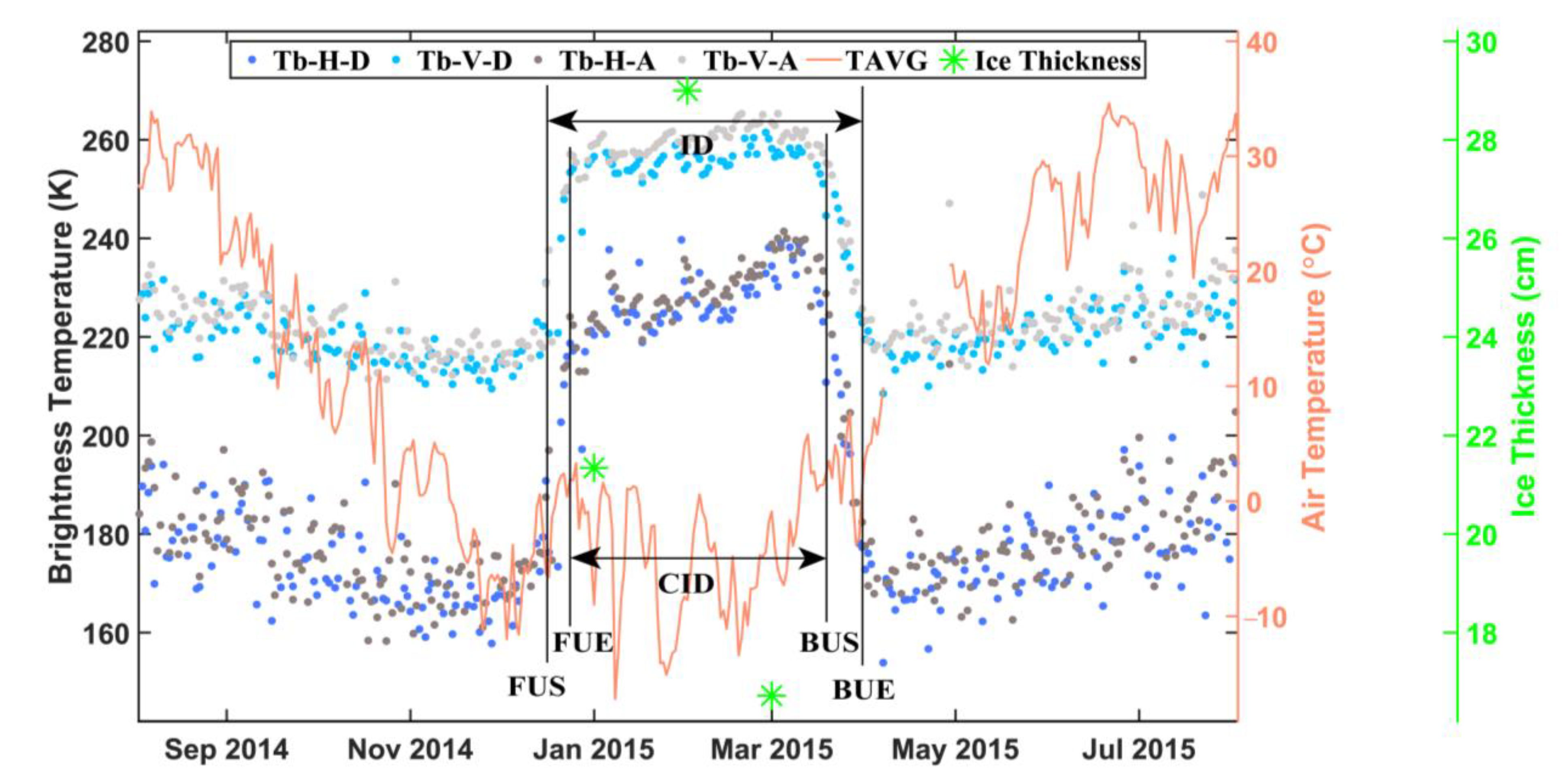
  • From August to December 2014, air temperature and Tb of Qinghai Lake both gradually decreased, but air temperature decreased faster;
  • Tb started to increase rapidly on December 13, which was the FUS. When Tb stabilized after a few days, the first date (23 December 2014) of the steady period was the FUE;
  • From January to March 2015, as ice thickness grew after the lake froze, the polarization difference decreased, and the Tb of the lake continued to increase slowly. On March 16, when the lake ice began to melt, the Tb started to decrease. Thus, March 16 is the BUS, from which Tb decreased with ice melting and air temperature increased until April 3; the BUE was recorded when the lake ice melted completely;
  • After April 3, Tb remained low while air temperature increased rapidly.
The Tb from the pixel of the lake geometric center point was chosen to represent the entire lake. For very large lakes with irregular shapes, such as Lake Baikal, Great Bear Lake, Great Slave Lake, Balkash Lake, and Lake Winnipeg, Tb was retrieved from multiple points in the lake, and the average Tb was used to calculate the lake ice phenology (Table A1).
Lake ice phenology can be extracted by automatic and manual methods. The automatic extraction method obtains the lake ice phenology by defining a certain threshold of Tb difference during the freezing and the break-up periods [17,20]. The method is highly efficient and time-saving, but most results need to be corrected manually. The manual identification method identifies lake ice phenology based on abrupt changes of Tb from the passive microwave Tb and lake characteristics; although the manual method is more time consuming, it is highly accurate. Systematic bias may influence Tb but would not influence the abrupt change. For the sake of accuracy, the ice phenology from the 22 lakes in this study was extracted through manual identification.

3.2. Validation Index

Lake observation data from GLRIPD and CIS products and manual identification from the MODIS products were used for validation and comparison. Statistical parameters, including coefficient of determination (R2), root mean square error (RMSE), mean absolute error (MAE), and mean bias error (MBE) were used to characterize the accuracy of ice phenology. These statistical parameters are described as:
R 2 = 1 i ( y m w y o b s ) 2 i ( y m w ¯ y o b s ) 2
R M S E = 1 m i = 1 m ( y o b s y m w ) 2
M A E = 1 m i = 1 m | y o b s y m w |
M B E = 1 m i = 1 m ( y o b s y m w )
where i is the ordinal year of the data, m is the total number of years (m = 40 in this study), ymw indicates lake ice phenology parameters retrieved from passive microwave remote sensing Tb data, while yobs is the annual lake ice phenology parameters obtained from observation data or other remote sensing products.

3.3. Prediction

Lake ice phenologies from 2021 to 2100 were predicted by multiple linear regression fitting with its climate-based driving factors. To simplify the process, the driving factors with the highest coefficient index were chosen to predict ice phenology. The prediction model has been formulated with lake ice phenology parameters retrieved from Tb variations and monthly air temperature, to ensure consistency in the resolution of the data with different representative concentration pathways (RCPs). For lake ice phenology parameters in each lake, an independent fitting formula was established as follows:
L I P = k 0 + k 1 T 1 m + k 2 T 2 m + + k n T n m
where kn represents the regression coefficient of lake ice phenology, n denotes the month, T n m epresents monthly air temperature data from CMIP5 historical data in 1979–2005 and RCP 2.6 data in 2006–2018, and m indicates the data types which include historical, RCP 2.6, 4.5, 6.0, and 8.5. LIP is the lake ice phenology parameters retrieved from Tb changes. After kn has been calculated, CMIP5 data of future scenarios in 2021–2100 were substituted as T n m into the equation to obtain the LIP for the same period.

4. Results

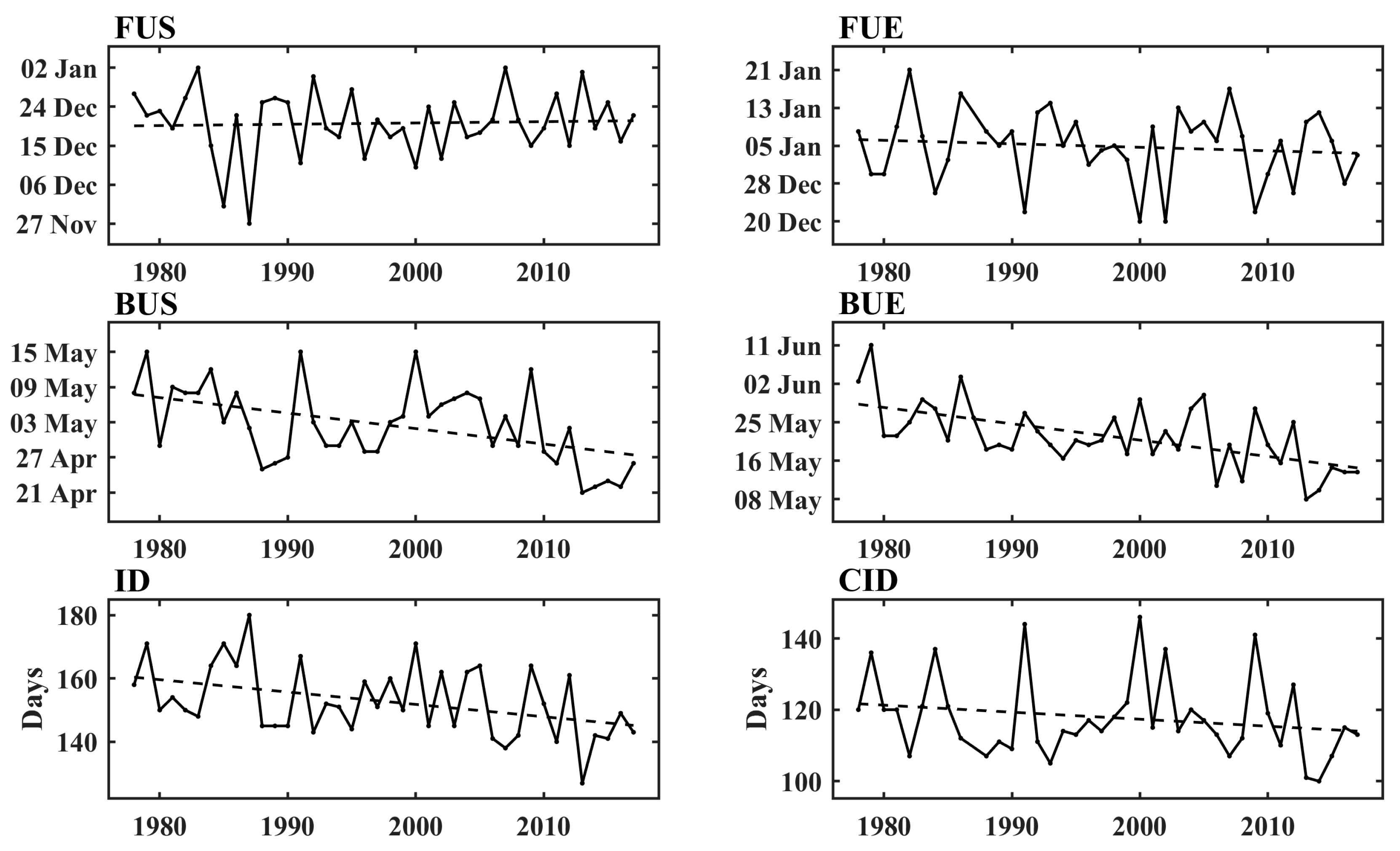
4.1. Variation of Lake Ice Phenology, 1979–2018

Six lake ice phenology parameters for 22 large lakes from 1979 to 2018 were calculated (Figure 4), and an F-test was performed to depict the significance of inter-annual change rate with certification level over 95%. In general, large lakes of the Northern Hemisphere had a delayed freezing period, earlier break-up period, and shortened ice duration. The FUS and FUE of most lakes were delayed. FUS was delayed in 21 lakes (91.3%), and FUE was delayed in 15 lakes (88.2%). There was an early trend in the break-up period. BUS was earlier in 20 lakes (87.0%), and BUE was earlier in 16 lakes (94.1%). The average change rate (ACR) of lake ice phenology, defined as a derivative from ice phenology parameters every year, showed that both FUS and FUE presented delayed trends by 0.23 days/year. Conversely, BUS and BUE had an earlier trend of −0.17 days/year and −0.33 days/year, respectively. The ACR of ID and CID were −0.67 days/year and −0.48 days/year, respectively. Among them, the number of lakes in which the ACR of FUS, FUE, BUS, BUE, ID, and CID passed the significance test (p < 0.05) was 7 (31.8%), 2 (9.1%), 10 (45.5%), 11 (50.0%), 14 (63.6%), and 9 (40.9%), respectively.
The number of lakes with a significant changing rate (p < 0.05) in the break-up period was much greater than that in the freezing period. The change rate of the break-up date was higher than that of the freezing date from 1979 to 2018 (Figure 5). The historical time series trends of well-known lakes were analyzed in different regions of the Northern Hemisphere, such as Lake Baikal, Qinghai Lake, Nam Co in Eurasia, and the Great Bear Lake, Great Slave Lake, Lake Winnipeg in North America (Lake Baikal is shown in Figure 6, other lakes are shown in Figure A2). The total areas of these lakes account for 61.0% of all lakes in the study area. Both FUS and FUE were delayed, and their average ACR was 0.14 days/year and 0.09 days/year, respectively. BUS and BUE had an earlier trend, and their average ACR was −0.21 days/year and −0.33 days/year, respectively. The average ACR of ID and CID were −0.47 days/year and −0.32 days/year, respectively, and were affected by the freezing period and break-up period simultaneously.
To quantify the spatio-temporal variability on different portions of the lakes, we selected Lake Baikal as an example. At first, we retrieved Tb from 23 points separated by about 25~30 km from north to south on Lake Baikal, following the spatial resolution of the passive microwave product. The lake ice phenology was hard to identify in five points (grey points in Figure 7) for their Tb fluctuations in both freeze-up period and break-up period. Therefore, these points were dropped, and the variability was based on the other 18 points. These points are sorted by latitude, with No. 1 located the most northeast. and No. 18 the most southwest (Figure 7). The average lake ice phenology parameters from 1979 to 2018 of these 18 points were calculated. There is an obvious trend from point No. 1 to No. 18. In the south of Lake Baikal, FUS, FUE are later, BUS, BUE are earlier, and ID, CID are shorter (Figure 8). The north of Lake Baikal shows an opposite pattern from the south. The FUS of No. 18 is later than No. 1 by 14.8 days, FUE is later by 22.3 days, BUS is earlier by 17.2 days, BUE is earlier by 15.9 days, ID is shorter by 31.7 days, and CID is shorter by 41.5 days.

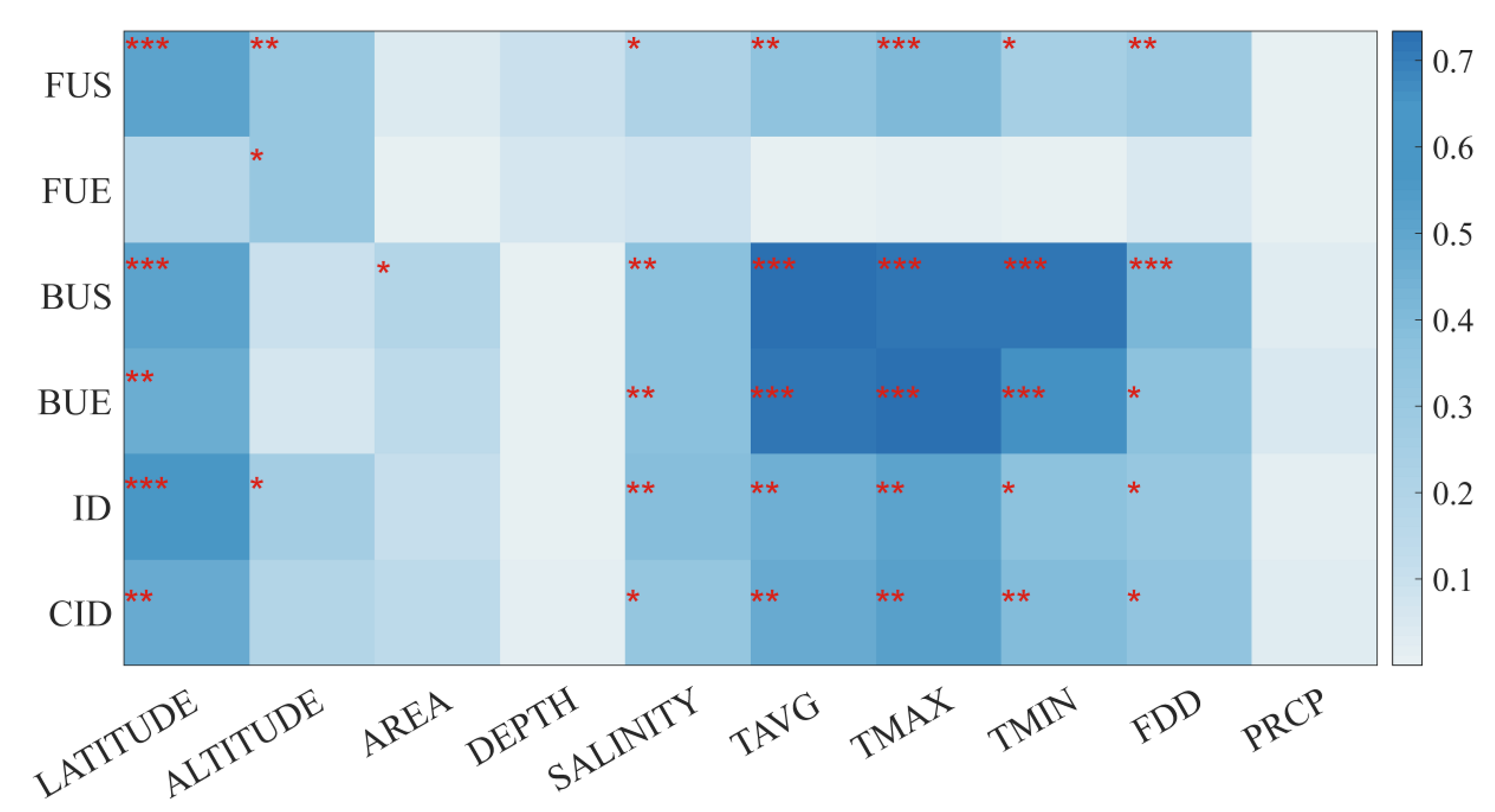
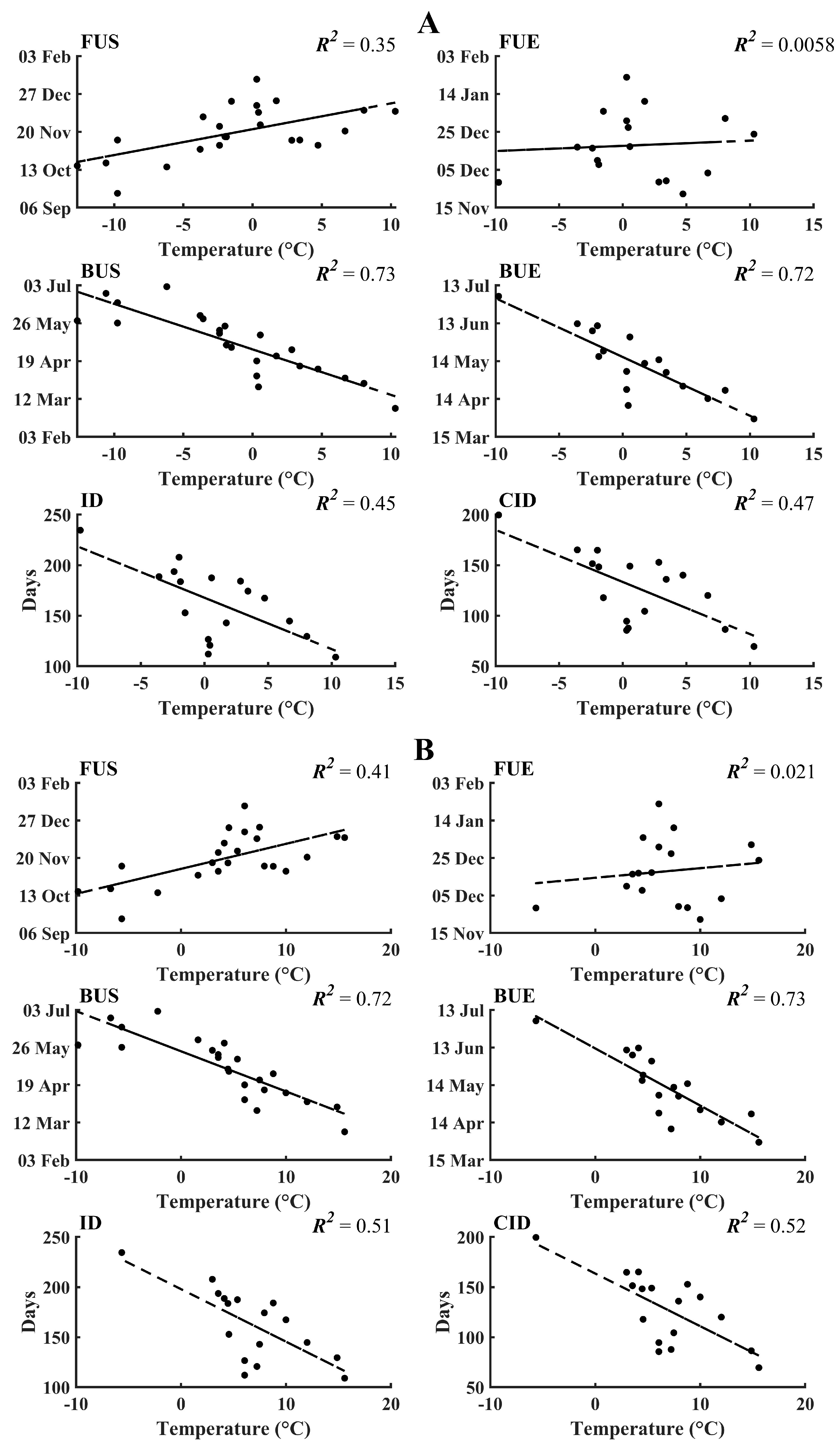
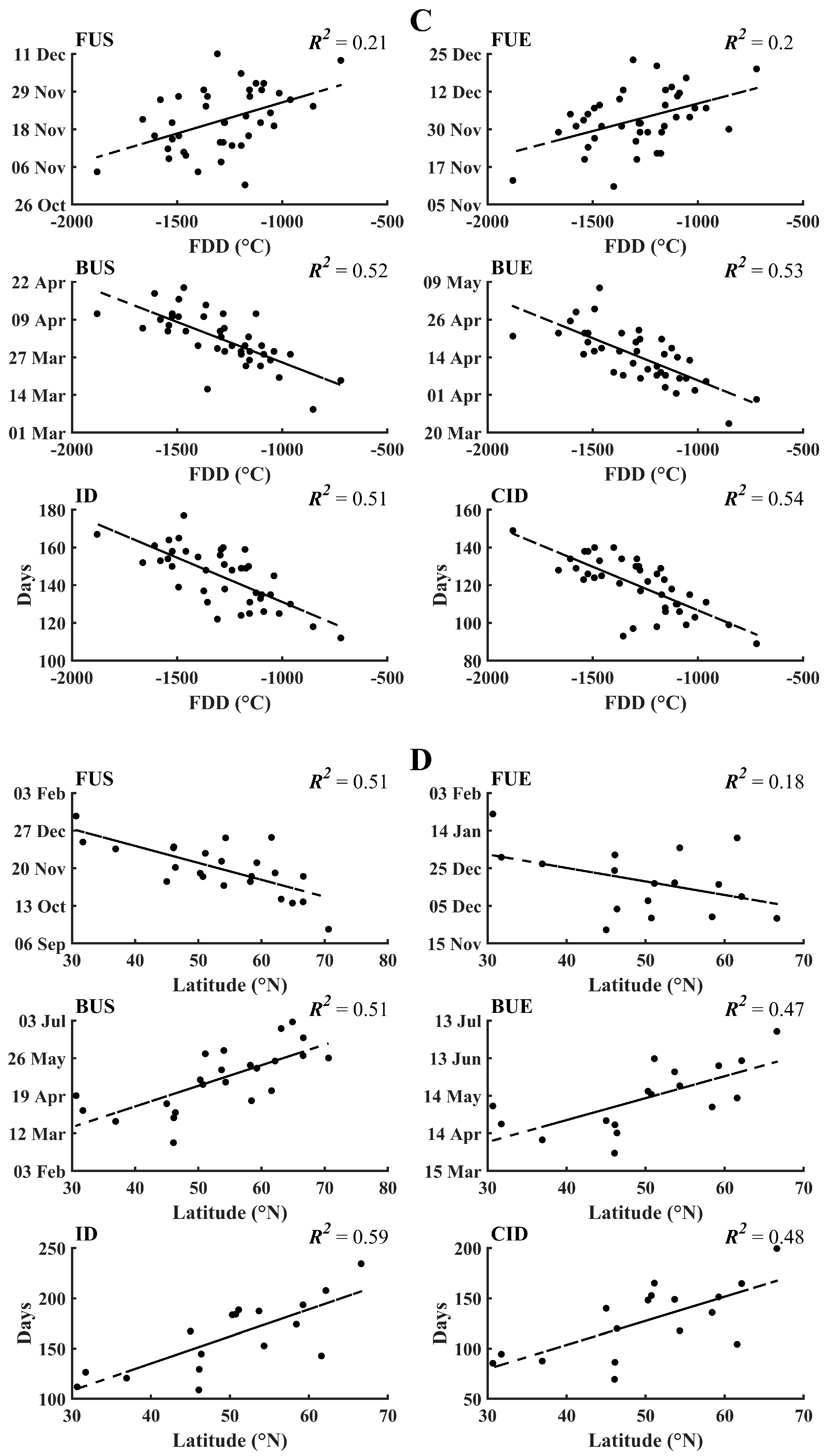
4.2. Driving Factors

Previous studies reported that latitude, surface area, volume, depth, salinity, air temperature, and precipitation are factors influencing lake ice phenology [12,19,26,30,35,36,84]. The quantitative relationships between lake ice phenology parameters and these factors were analyzed by linear regression, and the significance of these relationships was also calculated using the F-test with p < 0.05, p < 0.01, and p < 0.001. The air temperature observation data include annual average air temperature, annual maximum air temperature, annual minimum air temperature, and freezing degree days (FDD), which is the sum of average daily degrees below freezing for a year. In general, multiple factors comprehensively influence the interannual variations in lake ice phenology over the Northern Hemisphere. Among these factors, lake area, depth, and precipitation have little influence on ice phenology. Air temperature had the highest correlation with FUS, BUS, BUE, and CID, while latitude had the highest correlation with ID. Altitude was the only factor showing significant influence on FUE, with an R2 of 0.31 (Figure 9).
The coefficients of the break-up period were higher than that of the freezing period in all respects. The highest influencing factor of FUS was latitude, with a regression coefficient (R2) of 0.51. BUS and BUE were significantly influenced by air temperatures, latitude, and salinity. Among them, the average, maximum, and minimum air temperatures presented the largest influence on BUS and BUE. The R2 of average, maximum, minimum air temperatures with BUS were 0.73, 0.72, and 0.71, respectively. The R2 of average, maximum, minimum air temperatures with BUE were 0.72, 0.73, and 0.66, respectively. ID and CID were influenced by maximum air temperature, with an R2 of 0.51 and 0.52, respectively. As air temperature increased, FUS and FUE were delayed, BUS and BUE were earlier, and ID and CID became shorter (Figure A3).
The lakes located at higher latitude had earlier FUS and FUE, later BUS and BUE, and longer ID and CID. To investigate how much lake ice phenology was influenced by latitude, 22 lakes were grouped into three groups. Group A included lakes at a latitude below 50° N; group B was lakes between 50° N and 60° N; group C was lakes at latitudes greater than 60° N. In general, the interannual change rates of all lake ice phenology parameters in groups A and C were higher than group B, i.e., the change rates of lake ice phenology in low-latitude (<50° N) and high-latitude regions (>60° N) is higher than the mid-latitude (50° N ~ 60° N) region, which could be attributed to air temperature and polar amplification. Air temperature is the dominant factor in high annual change rates of lake ice phenology below the 50° N region, while polar amplification plays a greater role in the region above 60° N [11].

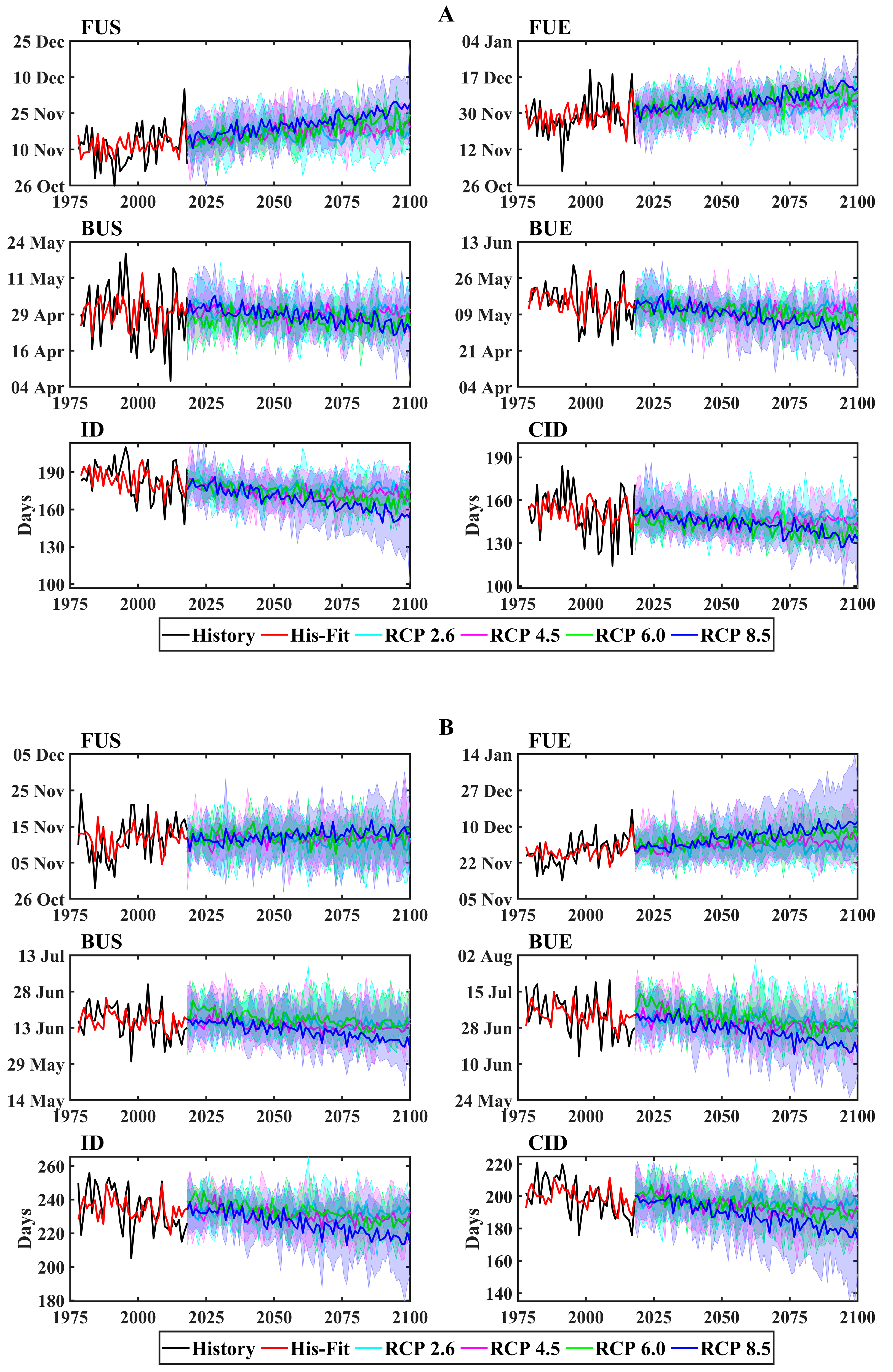
4.3. Variation of Lake Ice Phenology in the Future

According to the IPCC AR5 report, continued emissions of greenhouse gases will cause further global warming and long-lasting changes in all components of the climate system, increasing the likelihood of severe, pervasive, and irreversible impacts on people and ecosystems. Relative to 1850–1900, the global surface temperature change for the end of the 21st century (2081–2100) is projected to likely increase by 1.5 °C for RCP 4.5, RCP 6.0, and RCP 8.5 (high confidence) [1]. To project how lake ice will change at the hemispheric scale, the lake ice phenologies of 22 lakes in the period 2021–2100 were predicted by relating lake ice phenology and air temperature, which had the highest correlation coefficient among all factors.
Limited future change rates of lake ice phenologies of six well-known lakes were revealed in the low-emission pathways (RCPs 2.6 and 4.5), while higher change rates were found in the high-emission pathways (RCPs 6.0 and 8.5) (Lake Baikal is shown in Figure 10, other lakes are shown in Figure A4). Compared with lake ice phenology changes from 1990 to 2010, the average FUS of these 22 lakes from 2080 to 2100 will be delayed by 3.1 days in the RCP 2.6 scenario and 11.8 days in the RCP 8.5 scenario; the BUS will be earlier by 3.3 days in RCP 2.6. and 10.7 days in RCP 8.5; and the ID will be reduced by 6.5 days in RCP 2.6 and 21.9 days in RCP 8.5. Similar to the historical trends during the period 1979–2018, FUS and FUE from 2080 to 2100 will be delayed, BUS and BUE will be earlier, and ID and CID will shorten.
Analysis of ice phenology on a large number of lakes and rivers over the Northern Hemisphere demonstrated that the increase of 1 °C on mean air temperature would lead to a five-day decrease in ice cover duration [12,19,76]. Similar to previous research, the 1 °C increase in average air temperature will result in a 2.6-day delay on FUS, 2.7-day earlier BUS, and 5.3-day decrease in ID in this study.

5. Discussion

5.1. Validation with Site Observation

The GLRIPD sites observation data, including FUE and BUE, of four well-known lakes (Lake Baikal, Qinghai Lake, Lake Winnipeg, and Great Slave Lake) were used to validate lake ice phenology. Larger lakes have a greater impact on climate. FUE and BUE derived from passive microwave Tb were consistent with those from site observations. The smallest mean bias error (MBE) of FUE was 0.39 (comparison period was 1979 to 1990, Lake Winnipeg). The total MBE of FUE and BUE of these lakes was 7.96 and 3.65, respectively (Table 3). The deviation was mainly caused by the spatial heterogeneity of the freezing and thawing processes over large lakes (Figure 11). The passive microwave remote sensing data reflect the lake status over a large area, but the in situ observations refer to a point. For instance, the southernmost FUE was about 15 days later than the northernmost point of Great Slave Lake because the freezing process mainly starts from the northernmost areas. This heterogeneity in Qinghai Lake was lowest among the 22 lakes because the distance between the retrieval point and its weather station was the shortest of all.

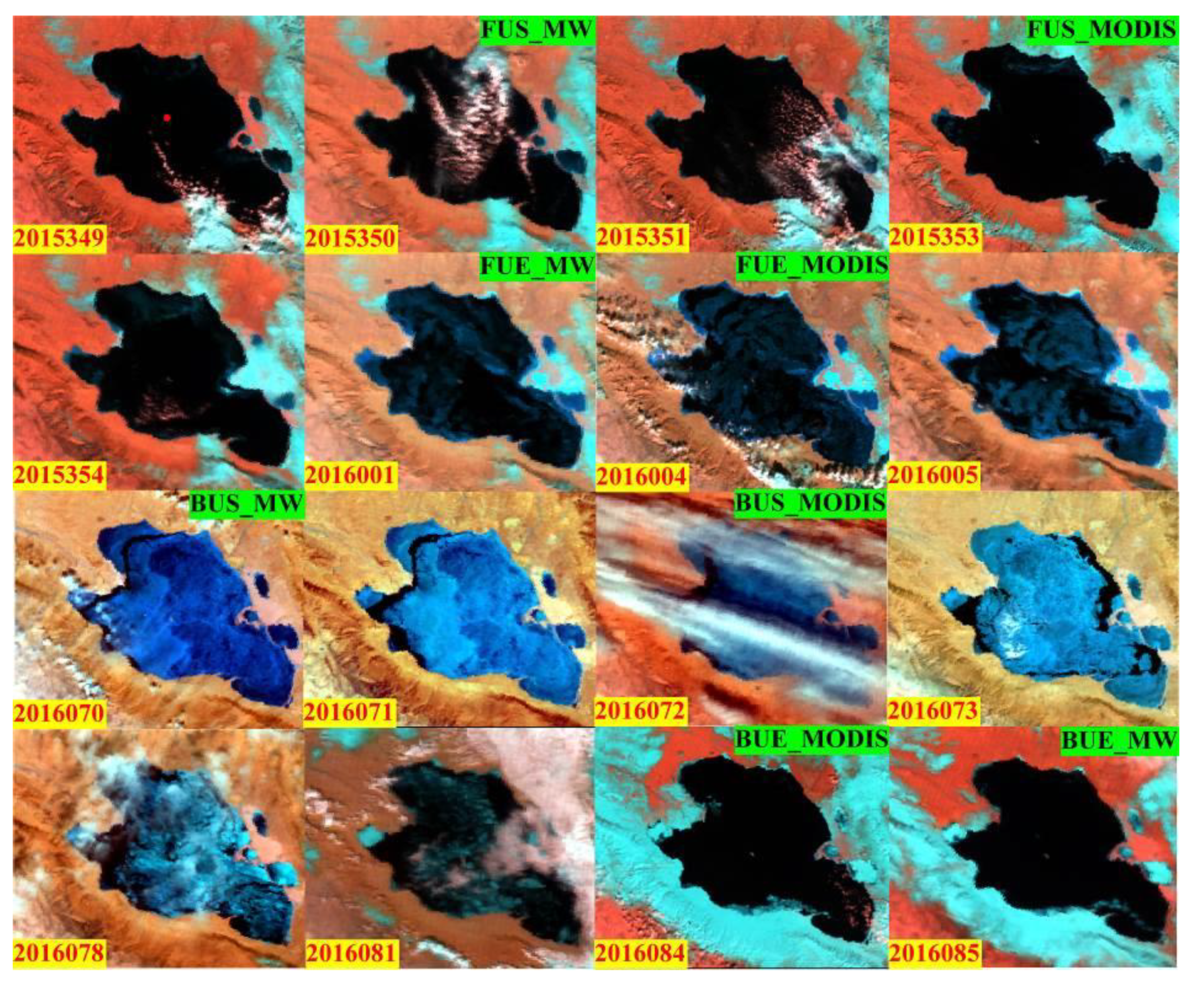
5.2. Comparison with Remote Sensing Products

The lake ice phenology was compared with visual interpretation from the MODIS surface reflectance product (MOD09GA, Collection 6) from 2015 to 2017, lake-wide ice product from the Canadian Ice Service (CIS) from 2000 to 2006 [15], and retrievals by other studies from passive microwave remote sensing in different periods (1979–2015 and 2002–2015).
Identifying the lake ice freezing process during the winter freezing period in higher latitude areas from optical images is difficult because optical remote sensing products are greatly affected by persistent cloud cover at low solar zenith angles [9,58,59,60]. As a result, only the BUS and BUE of lake ice of the Great Bear Lake, Great Slave Lake, Lake Baikal, Lake Winnipeg from the break-up period were retrieved (Figure A1). Qinghai Lake is in the mid-latitude region. Thus, all ice phenology parameters, FUS, FUE, BUS, BUE, ID, and CID, were retrieved (Figure 12). The MBE of BUS of these five lakes ranged from −0.11 to −2.67, and BUE was from −1 to −6.5. Overall, BUS and BUE during the break-up period in this study were earlier than those interpreted from MODIS. BUS was earlier by an average of 1.76 days, and BUE was earlier by an average of 3.13 days. These results are consistent with those reported in Cai, Ke and Duan [71]. Compared with the CIS product, the BUE of Great Bear Lake and Great Slave Lake showed an R2 of 0.94 and 0.75, respectively, but an MBE of −15.7 and −27, respectively (Table 4). The differences could be attributed to a sensor spatial resolution inconsistency of the CIS product with SMMR, SSM/I, and SSMIS. The SAR data used in the CIS product have a 100 m spatial resolution and seven-day temporal resolution. High R2 indicates the consistency of the time series trends despite systematic deviation. In general, the break-up period from passive microwave data was earlier than that from the optical remote sensing product, which could include frequent cloud contamination and have a different spatial resolution. In Qinghai Lake, the results were compared with those derived from AMSRE/2 in Qiu et al. [85] and those from SMMR and SSM/I in Cai, Ke and Duan [71] (Table 5). Compared with the result from AMSRE/2, the R2 values of FUS, FUE, BUS, and BUE are 0.11, 0.63, 0.94, and 0.91, respectively, while their MBEs are −9.64, −1.79, −2.14, and 3.21 days, respectively. Compared with the result of Cai, Ke and Duan [71], the R2 values of FUS, FUE, BUS and BUE are 0.18, 0.69, 0.81, and 0.77, respectively, while the MBEs are −5.35, −2.35, −4.00, and −1.32 days, respectively. The correlation between those results and this study is more consistent for the break-up period than for the freezing period.
Tb changed more regularly during the break-up period than the freezing period. It can be inferred that the ice near the lakeshore is hard to detect in terms of Tb variation; the freezing process is affected by weather variables such as wind. Different thresholds in the algorithms have greater inconsistencies, which leads to a relatively large deviation in the determination of the freezing period across studies. Furthermore, in some cases, the lake underwent a thaw–refreeze process in the break-up period that caused instability in the Tb value. Before BUE, the Tb value sometimes increased abruptly for a few days, then decreased. The thaw–refreeze process could be inferred from the Tb variation and could be attributed to the large fluctuations in air temperature during this period.

6. Conclusions

Six lake ice phenology parameters from 22 large lakes with areas greater than 625 km2 in the Northern Hemisphere have been derived from 18/19 GHz passive microwave Tb of SMMR, SSM/I, and SSMIS from forty ice seasons (1979–2018) by manual identification. The parameters included freeze-up start date (FUS), freeze-up end date (FUE) date, break-up start date (BUS), break-up end date (BUE) date, ice duration (ID), and complete ice duration (CID). There is a trend of significantly earlier ice break-up dates and decreasing ice duration in the last four decades. The freezing parameters (FUS, FUE) were both delayed by 0.23 days/year; the break-up parameters (BUS, BUE) were earlier by 0.17 and 0.33 days/year; and the duration parameters (ID, CID) were shortened by 0.67 and 0.48 days/year. The average change rate of BUE was higher than FUS, FUE, and BUS. The variation of lake ice phenology is the comprehensive effect of hydrology and climate change.
Latitude and air temperature may have a greater impact on lake ice phenology than other driving factors. The break-up parameters (BUS, BUE, ID, CID) were more strongly affected by air temperature than FUS and FUE. By establishing the relationship between lake ice phenology and air temperature, the variation of lake ice phenology in the period 2021–2100 were predicted under future climate change scenarios in different emission pathways. The ice duration will shorten by 6.5 days and 21.9 days under RCP 2.6 and RCP 8.5 scenarios, respectively, with global warming from 2021 to 2100 for the studied range at the hemispheric scale.
In this work, we studied the spatial pattern of large lakes’ ice phenology at the hemispheric scale; however, the spatiotemporal variabilities of ice phenology on different lake portions were analyzed on several special big lakes only. Recently, an improved, enhanced resolution, gridded passive microwave daily brightness temperature dataset had been published, which combined multiple sensors such as AMSRE, SMMR, SSM/I, and SSMIS, with higher spatial resolution at 3.125~25 km depending on different frequencies [86]. This provides a new opportunity to study the more detailed spatial characteristics of lake ice phenology in large lakes, as well as the lake ice phenology of those smaller lakes.

Author Contributions

Conceptualization, T.C.; funding acquisition, T.C. and L.D.; investigation, L.S.; software, L.S.; validation, L.S.; visualization, L.S.; writing—original draft preparation, L.S.; writing—review and editing, T.C. and L.D.; supervision, T.C.; All authors have read and agreed to the published version of the manuscript.

Funding

This study was funded by the Strategic Priority Research Program of the Chinese Academy of Sciences (grant no. XDA19070101), the National Natural Science Foundation of China (grant no. 41771389), and the CAS ‘Light of West China’ Program (grant no. E029070101).

Institutional Review Board Statement

Not applicable.

Informed Consent Statement

Not applicable.

Data Availability Statement

The retrieved lake ice phenology data are available from the corresponding author.

Acknowledgments

The authors would like to acknowledge the National Snow and Ice Data Center (NSIDC), the Canadian Ice Service (CIS), the World Wildlife Fund (WWF), and the International Lake Environment Committee Foundation (ILEC), who provided data related to this paper. We also acknowledge the World Climate Research Programme’s Working Group on Coupled Modelling, which is responsible for CMIP, and we thank the climate modeling groups (listed in Table 2 of this paper) for producing and making their model outputs available. Finally, we would like to thank the reviewers for providing useful and insightful feedback.

Conflicts of Interest

The authors declare no conflict of interest.

Appendix A

Table A1. Coordinates of the Tb retrieval points of five lakes: Lake Baikal, Great Bear Lake, Great Slave Lake, Lake Winnipeg, and Balkhash Lake.
Lake NamePixel IDLatitudeLongitude
Lake BaikalBK-155.341° N109.520° E
BK-255.123° N109.427° E
BK-354.819° N109.306° E
BK-454.562° N109.170° E
BK-554.303° N109.047° E
BK-654.073° N108.785° E
BK-753.874° N108.510° E
BK-853.192° N108.003° E
BK-953.006° N107.789° E
BK-1052.878° N107.511° E
BK-1152.814° N107.204° E
BK-1252.731° N106.922° E
BK-1352.375° N106.169° E
BK-1452.110° N105.951° E
BK-1551.928° N105.680° E
BK-1651.796° N105.391° E
BK-1751.714° N105.055° E
BK-1851.639° N104.348° E
Great Bear LakeGB-166.614° N120.829° W
GB-265.783° N120.805° W
GB-365.285° N122.325° W
GB-466.092° N118.288° W
Great Slave LakeGS-162.151° N114.561° W
GS-261.628° N113.587° W
GS-361.035° N115.605° W
GS-461.415° N114.513° W
Lake WinnipegWI-153.535° N98.457° W
WI-252.447° N97.617° W
Balkhash LakeBA-146.376° N74.600° E
BA-245.792° N73.935° E
Figure A1. MODIS images (MOD09GA) of lake ice break-up in one year of Great Bear Lake (A), Great Slave Lake (B), Lake Winnipeg (C), and Lake Baikal (D). Red dots in the first image of each sub figure denote the coordinates of the Tb retrieval points of each lake. The 6-2-1 band combination is shown in RGB view. To be noted, BUE_MW in Great Slave Lake is 2016149; in Lake Winnipeg, BUE_MODIS is 2017140, BUE_MW is 2017142; in Lake Baikal, BUS_MW is 2016114, which is fully covered by clouds and it is not shown. The abbreviations are as follows: FUS, freeze-up start date; FUE, freeze-up end date; BUS, break-up start date; BUE, break-up end date. “MW” denotes that this image is from microwave remote sensing in this study, “MODIS” means the result was obtained from the MODIS surface reflectance product.
Remotesensing 13 01389 g0a1aRemotesensing 13 01389 g0a1b
Figure A2. Variation in lake ice phenology of five typical lakes (1979–2018): Lake Winnipeg (A), Great Bear Lake (B), Great Slave Lake (C), Qinghai Lake (D), and Nam Co (E). FUS, freeze-up start date; FUE, freeze-up end date; BUS, break-up start date; BUE, break-up end date; ID, ice duration; CID, complete ice duration.
Remotesensing 13 01389 g0a2aRemotesensing 13 01389 g0a2b
Figure A3. Correlation between lake ice phenology and annual average air temperature (A), annual maximum air temperature (B), freezing degree days (FDD) (C), and latitude (D). The annual maximum air temperature is averaged based on daily data. FUS, freeze-up start date; FUE, freeze-up end date; BUS, break-up start date; BUE, break-up end date; ID, ice duration; CID, complete ice duration.
Remotesensing 13 01389 g0a3aRemotesensing 13 01389 g0a3b
Figure A4. Interannual variations of lake ice phenology of five well-known lakes from 1979 to 2100: Lake Winnipeg (A), Great Bear Lake (B), Great Slave Lake (C), Qinghai Lake (D), and Nam Co (E). The abbreviations are explained in Figure 10.
Remotesensing 13 01389 g0a4aRemotesensing 13 01389 g0a4bRemotesensing 13 01389 g0a4c

References

  1. Pachauri, R.K.; Allen, M.R.; Barros, V.R.; Broome, J.; Cramer, W.; Christ, R.; Church, J.A.; Clarke, L.; Dahe, Q.; Dasgupta, P.; et al. IPCC, 2014: Climate Change 2014: Synthesis Report; Contribution of Working Groups I, II and III to the Fifth Assessment Report of the Intergovernmental Panel on Climate Change; IPCC: Geneva, Switzerland, 2014; p. 151. [Google Scholar]
  2. World Meteorological Organization. The Global Observing System For Climate: Implementation Needs (GCOS-200). In GCOS 2016 Implementation Plan; World Meteorological Organization: Geneva, Switzerland, 2016; p. 9. [Google Scholar]
  3. Brown, L.C.; Duguay, C.R. The response and role of ice cover in lake-climate interactions. Prog. Phys. Geog. 2010, 34, 671–704. [Google Scholar] [CrossRef]
  4. Duguay, C.R.; Prowse, T.D.; Bonsal, B.R.; Brown, R.D.; Lacroix, M.P.; Menard, P. Recent trends in Canadian lake ice cover. Hydrol. Process. 2006, 20, 781–801. [Google Scholar] [CrossRef]
  5. Williams, G.P. Predicting the Date of Lake Ice Breakup. Water Resour. Res. 1971, 7, 323–333. [Google Scholar] [CrossRef] [Green Version]
  6. Livingstone, D.M. Break-up dates of Alpine lakes as proxy data for local and regional mean surface air temperatures. Clim. Chang. 1997, 37, 407–439. [Google Scholar] [CrossRef] [Green Version]
  7. Weber, H.; Riffler, M.; Noges, T.; Wunderle, S. Lake ice phenology from AVHRR data for European lakes: An automated two-step extraction method. Remote Sens. Environ. 2016, 174, 329–340. [Google Scholar] [CrossRef]
  8. Adrian, R.; O’Reilly, C.M.; Zagarese, H.; Baines, S.B.; Hessen, D.O.; Keller, W.; Livingstone, D.M.; Sommaruga, R.; Straile, D.; Van Donk, E.; et al. Lakes as sentinels of climate change. Limnol. Oceanogr. 2009, 54, 2283–2297. [Google Scholar] [CrossRef] [PubMed]
  9. Duguay, C.R.; Bernier, M.; Gauthier, Y.; Kouraev, A. Remote sensing of lake and river ice. In Remote Sensing of the Cryosphere; Wiley Blackwell: Hoboken, NJ, USA, 2015; pp. 273–306. [Google Scholar] [CrossRef]
  10. Mishra, V.; Cherkauer, K.A.; Bowling, L.C.; Huber, M. Lake Ice phenology of small lakes: Impacts of climate variability in the Great Lakes region. Glob. Planet. Chang. 2011, 76, 166–185. [Google Scholar] [CrossRef]
  11. Du, J.Y.; Kimball, J.S.; Duguay, C.; Kim, Y.; Watts, J.D. Satellite microwave assessment of Northern Hemisphere lake ice phenology from 2002 to 2015. Cryosphere 2017, 11, 47–63. [Google Scholar] [CrossRef] [Green Version]
  12. Magnuson, J.J.; Robertson, D.M.; Benson, B.J.; Wynne, R.H.; Livingstone, D.M.; Arai, T.; Assel, R.A.; Barry, R.G.; Card, V.; Kuusisto, E.; et al. Historical trends in lake and river ice cover in the Northern Hemisphere. Science 2000, 289, 1743–1746. [Google Scholar] [CrossRef] [Green Version]
  13. Latifovic, R.; Pouliot, D. Analysis of climate change impacts on lake ice phenology in Canada using the historical satellite data record. Remote Sens. Environ. 2007, 106, 492–507. [Google Scholar] [CrossRef]
  14. Prowse, T.; Alfredsen, K.; Beltaos, S.; Bonsal, B.; Duguay, C.; Korhola, A.; McNamara, J.; Pienitz, R.; Vincent, W.F.; Vuglinsky, V.; et al. Past and Future Changes in Arctic Lake and River Ice. Ambio 2011, 40, 53–62. [Google Scholar] [CrossRef] [Green Version]
  15. Howell, S.E.L.; Brown, L.C.; Kang, K.K.; Duguay, C.R. Variability in ice phenology on Great Bear Lake and Great Slave Lake, Northwest Territories, Canada, from SeaWinds/QuikSCAT: 2000–2006. Remote Sens. Environ. 2009, 113, 816–834. [Google Scholar] [CrossRef]
  16. Kang, K.K.; Duguay, C.R.; Howell, S.E.L. Estimating ice phenology on large northern lakes from AMSR-E: Algorithm development and application to Great Bear Lake and Great Slave Lake, Canada. Cryosphere 2012, 6, 235–254. [Google Scholar] [CrossRef] [Green Version]
  17. Che, T.; Li, X.; Jin, R. Monitoring the frozen duration of Qinghai Lake using satellite passive microwave remote sensing low frequency data. Chin. Sci. Bull. 2009, 54, 2294–2299. [Google Scholar] [CrossRef]
  18. Ke, C.Q.; Tao, A.Q.; Jin, X. Variability in the ice phenology of Nam Co Lake in central Tibet from scanning multichannel microwave radiometer and special sensor microwave/imager: 1978 to 2013. J. Appl. Remote Sens. 2013, 7. [Google Scholar] [CrossRef]
  19. Yao, X.J.; Li, L.; Zhao, J.; Sun, M.P.; Li, J.; Gong, P.; An, L.N. Spatial-temporal variations of lake ice phenology in the Hoh Xil region from 2000 to 2011. J. Geogr. Sci. 2016, 26, 70–82. [Google Scholar] [CrossRef]
  20. Qiu, Y.; Wang, X.; Ruan, Y.; Xie, P.; Zhong, Y.; Yang, S. Passive microwave remote sensing of lake freeze-thawing over Qinghai-Tibet Plateau. J. Lake Sci. 2018, 30, 1438–1449. (In Chinese) [Google Scholar] [CrossRef]
  21. Qi, M.M.; Liu, S.Y.; Yao, X.J.; Xie, F.M.; Gao, Y.P. Monitoring the Ice Phenology of Qinghai Lake from 1980 to 2018 Using Multisource Remote Sensing Data and Google Earth Engine. Remote Sens. 2020, 12, 2217. [Google Scholar] [CrossRef]
  22. Gou, P.; Ye, Q.H.; Che, T.; Feng, Q.; Ding, B.H.; Lin, C.G.; Zong, J.B. Lake ice phenology of Nam Co, Central Tibetan Plateau, China, derived from multiple MODIS data products. J. Great Lakes Res. 2017, 43, 989–998. [Google Scholar] [CrossRef]
  23. Veillette, J.; Muir, D.C.G.; Antoniades, D.; Small, J.M.; Spencer, C.; Loewen, T.N.; Babaluk, J.A.; Reist, J.D.; Vincent, W.F. Perfluorinated Chemicals in Meromictic Lakes on the Northern Coast of Ellesmere Island, High Arctic Canada. Arctic 2012, 65, 245–256. [Google Scholar] [CrossRef] [Green Version]
  24. Wrona, F.J.; Johansson, M.; Culp, J.M.; Jenkins, A.; Mard, J.; Myers-Smith, I.H.; Prowse, T.D.; Vincent, W.F.; Wookey, P.A. Transitions in Arctic ecosystems: Ecological implications of a changing hydrological regime. J. Geophys. Res. Biogeo 2016, 121, 650–674. [Google Scholar] [CrossRef] [Green Version]
  25. Greene, S.; Anthony, K.M.W.; Archer, D.; Sepulveda-Jauregui, A.; Martinez-Cruz, K. Modeling the impediment of methane ebullition bubbles by seasonal lake ice. Biogeosciences 2014, 11, 6791–6811. [Google Scholar] [CrossRef] [Green Version]
  26. Weyhenmeyer, G.A.; Livingstone, D.M.; Meili, M.; Jensen, O.; Benson, B.; Magnuson, J.J. Large geographical differences in the sensitivity of ice-covered lakes and rivers in the Northern Hemisphere to temperature changes. Glob. Change Biol. 2011, 17, 268–275. [Google Scholar] [CrossRef]
  27. Sharma, S.; Blagrave, K.; Magnuson, J.J.; O’Reilly, C.M.; Oliver, S.; Batt, R.D.; Magee, M.R.; Straile, D.; Weyhenmeyer, G.A.; Winslow, L.; et al. Widespread loss of lake ice around the Northern Hemisphere in a warming world. Nat. Clim. Change 2019, 9, 227–231. [Google Scholar] [CrossRef]
  28. Schroter, D.; Cramer, W.; Leemans, R.; Prentice, I.C.; Araujo, M.B.; Arnell, N.W.; Bondeau, A.; Bugmann, H.; Carter, T.R.; Gracia, C.A.; et al. Ecosystem service supply and vulnerability to global change in Europe. Science 2005, 310, 1333–1337. [Google Scholar] [CrossRef] [PubMed] [Green Version]
  29. Todd, M.C.; Mackay, A.W. Large-scale climatic controls on Lake Baikal ice cover. J. Clim. 2003, 16, 3186–3199. [Google Scholar] [CrossRef]
  30. Kouraev, A.V.; Semovski, S.V.; Shimaraev, M.N.; Mognard, N.M.; Legresy, B.; Remy, F. Observations of Lake Baikal ice from satellite altimetry and radiometry. Remote Sens. Environ. 2007, 108, 240–253. [Google Scholar] [CrossRef]
  31. Benson, B.J.; Magnuson, J.J.; Jensen, O.P.; Card, V.M.; Hodgkins, G.; Korhonen, J.; Livingstone, D.M.; Stewart, K.M.; Weyhenmeyer, G.A.; Granin, N.G. Extreme events, trends, and variability in Northern Hemisphere lake-ice phenology (1855–2005). Clim. Change 2012, 112, 299–323. [Google Scholar] [CrossRef]
  32. Liston, G.E.; Hall, D.K. Sensitivity of lake freeze-up and break-up to climate change: A physically based modeling study. Ann. Glaciol. 1995, 21, 387–393. [Google Scholar] [CrossRef] [Green Version]
  33. Walsh, S.E.; Vavrus, S.J.; Foley, J.A.; Fisher, V.A.; Wynne, R.H.; Lenters, J.D. Global patterns of lake ice phenology and climate: Model simulations and observations. J. Geophys. Res. Atmos. 1998, 103, 28825–28837. [Google Scholar] [CrossRef] [Green Version]
  34. O’Reilly, C.M.; Sharma, S.; Gray, D.K.; Hampton, S.E.; Read, J.S.; Rowley, R.J.; Schneider, P.; Lenters, J.D.; McIntyre, P.B.; Kraemer, B.M.; et al. Rapid and highly variable warming of lake surface waters around the globe. Geophys. Res. Lett. 2015, 42, 10773–10781. [Google Scholar] [CrossRef] [Green Version]
  35. Menard, P.; Duguay, C.R.; Flato, G.M.; Rouse, W.R. Simulation of ice phenology on Great Slave Lake, Northwest Territories, Canada. Hydrol. Process. 2002, 16, 3691–3706. [Google Scholar] [CrossRef]
  36. Qi, M.M.; Yao, X.J.; Li, X.F.; Duan, H.Y.; Gao, Y.P.; Liu, J. Spatiotemporal characteristics of Qinghai Lake ice phenology between 2000 and 2016. J. Geogr. Sci. 2019, 29, 115–130. [Google Scholar] [CrossRef] [Green Version]
  37. Wilson, J.W. Effect of Lake-Ontario on Precipitation. Mon. Weather. Rev. 1977, 105, 207–214. [Google Scholar] [CrossRef]
  38. Zhang, G.; Chen, W.; Li, G.; Yang, W.; Yi, S.; Luo, W. Lake water and glacier mass gains in the northwestern Tibetan Plateau observed from multi-sensor remote sensing data: Implication of an enhanced hydrological cycle. Remote Sens. Environ. 2020, 237, 111554. [Google Scholar] [CrossRef]
  39. Liu, Y.; Chen, H.P.; Li, H.X.; Wang, H.J. The Impact of Preceding Spring Antarctic Oscillation on the Variations of Lake Ice Phenology over the Tibetan Plateau. J. Clim. 2020, 33, 639–656. [Google Scholar] [CrossRef]
  40. Liu, Y.; Chen, H.P.; Wang, H.J.; Qiu, Y.B. The Impact of the NAO on the Delayed Break-Up Date of Lake Ice over the Southern Tibetan Plateau. J. Clim. 2018, 31, 9073–9086. [Google Scholar] [CrossRef]
  41. Park, H.; Yoshikawa, Y.; Oshima, K.; Kim, Y.; Thanh, N.D.; Kimball, J.S.; Yang, D.Q. Quantification of Warming Climate-Induced Changes in Terrestrial Arctic River Ice Thickness and Phenology. J. Clim. 2016, 29, 1733–1754. [Google Scholar] [CrossRef]
  42. Yang, X.; Pavelsky, T.M.; Allen, G.H. The past and future of global river ice. Nature 2020, 577, 69–73. [Google Scholar] [CrossRef]
  43. Dibike, Y.; Prowse, T.; Bonsal, B.; de Rham, L.; Saloranta, T. Simulation of North American lake-ice cover characteristics under contemporary and future climate conditions. Int. J. Clim. 2012, 32, 695–709. [Google Scholar] [CrossRef]
  44. Sharma, S.; Magnuson, J.J.; Batt, R.D.; Winslow, L.A.; Korhonen, J.; Aono, Y. Direct observations of ice seasonality reveal changes in climate over the past 320–570 years. Sci. Rep. 2016, 6, 25061. [Google Scholar] [CrossRef] [Green Version]
  45. Chaouch, N.; Temimi, M.; Romanov, P.; Cabrera, R.; McKillop, G.; Khanbilvardi, R. An automated algorithm for river ice monitoring over the Susquehanna River using the MODIS data. Hydrol. Process. 2014, 28, 62–73. [Google Scholar] [CrossRef]
  46. Kropacek, J.; Maussion, F.; Chen, F.; Hoerz, S.; Hochschild, V. Analysis of ice phenology of lakes on the Tibetan Plateau from MODIS data. Cryosphere 2013, 7, 287–301. [Google Scholar] [CrossRef] [Green Version]
  47. Liu, X.D.; Chen, B.D. Climatic warming in the Tibetan Plateau during recent decades. Int. J. Clim. 2000, 20, 1729–1742. [Google Scholar] [CrossRef]
  48. Shiklomanov, A.I.; Lammers, R.B.; Vörösmarty, C.J. Widespread decline in hydrological monitoring threatens Pan-Arctic Research. EOS 2002, 83, 13–17. [Google Scholar] [CrossRef]
  49. Richard, S.; Williams, J.; Ferrigno, G. State of the Earth’s Cryosphere at the Beginning of the 21st Century—Glaciers, Global Snow Cover, Floating Ice, and Permafrost and Periglacial Environments; U.S. Geological Survey; US Government: Washington, DC, USA, 2012; 546p.
  50. Lenormand, F.; Duguay, C.R.; Gauthier, R. Development of a historical ice database for the study of climate change in Canada. Hydrol. Process. 2002, 16, 3707–3722. [Google Scholar] [CrossRef]
  51. Nonaka, T.; Matsunaga, T.; Hoyano, A. Estimating ice breakup dates on Eurasian lakes using water temperature trends and threshold surface temperatures derived from MODIS data. Int. J. Remote Sens. 2007, 28, 2163–2179. [Google Scholar] [CrossRef]
  52. Hall, D.K.; Riggs, G.A.; Foster, J.L.; Kumar, S.V. Development and evaluation of a cloud-gap-filled MODIS daily snow-cover product. Remote Sens. Environ. 2010, 114, 496–503. [Google Scholar] [CrossRef] [Green Version]
  53. Hall, D.K.; Riggs, G.A. Accuracy assessment of the MODIS snow products. Hydrol. Process. 2007, 21, 1534–1547. [Google Scholar] [CrossRef]
  54. Pour, H.K.; Duguay, C.R.; Martynov, A.; Brown, L.C. Simulation of surface temperature and ice cover of large northern lakes with 1-D models: A comparison with MODIS satellite data and in situ measurements. Tellus A Dyn. Meteorol. Oceanogr. 2012, 64. [Google Scholar] [CrossRef] [Green Version]
  55. Cai, Y.; Ke, C.Q.; Li, X.G.; Zhang, G.Q.; Duan, Z.; Lee, H. Variations of Lake Ice Phenology on the Tibetan Plateau From 2001 to 2017 Based on MODIS Data. J. Geophys. Res. Atmos 2019, 124, 825–843. [Google Scholar] [CrossRef]
  56. Zhang, S.; Pavelsky, T.M. Remote Sensing of Lake Ice Phenology across a Range of Lakes Sizes, ME, USA. Remote Sens. 2019, 11, 1718. [Google Scholar] [CrossRef] [Green Version]
  57. Gafurov, A.; Bardossy, A. Cloud removal methodology from MODIS snow cover product. Hydrol. Earth Syst. Sci. 2009, 13, 1361–1373. [Google Scholar] [CrossRef] [Green Version]
  58. Maslanik, J.A.; Barry, R.G. The Influence of Climate Change and Climatic Variability on the Hydrologie Regime and Water Resources. In Proceedings of the Vancouver Symposium, Vancouver, BC, Canada, 9–22 August 1987. [Google Scholar]
  59. Jeffries, M.O.; Morris, K.; Kozlenko, N. Ice Characteristics and Processes, and Remote Sensing of Frozen Rivers and Lakes; American Geophysical Union: Washington, DC, USA, 2005. [Google Scholar]
  60. Smejkalova, T.; Edwards, M.E.; Dash, J. Arctic lakes show strong decadal trend in earlier spring ice-out. Sci. Rep. 2016, 6. [Google Scholar] [CrossRef] [PubMed]
  61. Hoekstra, M.; Jiang, M.Z.; Clausi, D.A.; Duguay, C. Lake Ice-Water Classification of RADARSAT-2 Images by Integrating IRGS Segmentation with Pixel-Based Random Forest Labeling. Remote Sens. 2020, 12, 1425. [Google Scholar] [CrossRef]
  62. Tom, M.; Kälin, U.; Sütterlin, M.; Baltsavias, E.; Schindler, K. Lake Ice Detection in Low-Resolution Optical Stellite Images. ISPR.S Ann. Photogramm. Remote Sens. Spat. Inf. Sci. 2018, IV-2, 279–286. [Google Scholar] [CrossRef] [Green Version]
  63. Wu, Y.; Duguay, C.R.; Xu, L. Assessment of machine learning classifiers for global lake ice cover mapping from MODIS TOA reflectance data. Remote Sens. Environ. 2021, 253, 112206. [Google Scholar] [CrossRef]
  64. Jeffries, M.O.; Morris, K.; Weeks, W.F.; Wakabayashi, H. Structural and Stratigraphic Features and Ers-1 Synthetic-Aperture Radar Backscatter Characteristics of Ice Growing on Shallow Lakes in Nw Alaska, Winter 1991–1992. J. Geophys. Res. Ocean. 1994, 99, 22459–22471. [Google Scholar] [CrossRef]
  65. Duguay, C.R.; Pultz, T.J.; Lafleur, P.M.; Drai, D. RADARSAT backscatter characteristics of ice growing on shallow sub-Arctic lakes, Churchill, Manitoba, Canada. Hydrol. Process. 2002, 16, 1631–1644. [Google Scholar] [CrossRef]
  66. Duguay, C.R.; Lafleur, P.M. Determining depth and ice thickness of shallow sub-Arctic lakes using space-borne optical and SAR data. Int. J. Remote Sens. 2003, 24, 475–489. [Google Scholar] [CrossRef]
  67. Surdu, C.M.; Duguay, C.R.; Pour, H.K.; Brown, L.C. Ice Freeze-up and Break-up Detection of Shallow Lakes in Northern Alaska with Spaceborne SAR. Remote Sens. 2015, 7, 6133–6159. [Google Scholar] [CrossRef] [Green Version]
  68. Dornhofer, K.; Oppelt, N. Remote sensing for lake research and monitoring—Recent advances. Ecol. Indic. 2016, 64, 105–122. [Google Scholar] [CrossRef]
  69. Cavalieri, D.J.; Gloersen, P.; Campbell, W.J. Determination of Sea Ice Parameters with the Nimbus-7 Smmr. J. Geophys. Res. Atmos. 1984, 89, 5355–5369. [Google Scholar] [CrossRef]
  70. Helfrich, S.R.; McNamara, D.; Ramsay, B.H.; Baldwin, T.; Kasheta, T. Enhancements to, and forthcoming developments in the Interactive Multisensor Snow and Ice Mapping System (IMS). Hydrol. Process. 2007, 21, 1576–1586. [Google Scholar] [CrossRef]
  71. Cai, Y.; Ke, C.Q.; Duan, Z. Monitoring ice variations in Qinghai Lake from 1979 to 2016 using passive microwave remote sensing data. Sci. Total Environ. 2017, 607–608, 120–131. [Google Scholar] [CrossRef] [PubMed]
  72. Kang, K.K.; Duguay, C.R.; Lemmetyinen, J.; Gel, Y. Estimation of ice thickness on large northern lakes from AMSR-E brightness temperature measurements. Remote Sens. Environ. 2014, 150, 1–19. [Google Scholar] [CrossRef]
  73. Messager, M.L.; Lehner, B.; Grill, G.; Nedeva, I.; Schmitt, O. Estimating the volume and age of water stored in global lakes using a geo-statistical approach. Nat. Commun. 2016, 7, 13603. [Google Scholar] [CrossRef]
  74. Lehner, B.; Doll, P. Development and validation of a global database of lakes, reservoirs and wetlands. J. Hydrol. 2004, 296, 1–22. [Google Scholar] [CrossRef]
  75. Global Lakes and Wetlands Database. Available online: https://www.worldwildlife.org/pages/global-lakes-and-wetlands-database (accessed on 8 March 2021).
  76. ILEC World Lake Database. Available online: https://wldb.ilec.or.jp/ (accessed on 8 March 2021).
  77. Global Lake Database. Available online: http://www.worldlakes.org/index.asp (accessed on 8 March 2021).
  78. Knowles, K.; Njoku, E.G.; Armstrong, R.; Brodzik, M.J. Nimbus-7 SMMR Pathfinder Daily EASE-Grid Brightness Temperatures. Version 1; NASA National Snow and Ice Data Center Distributed Active Archive Center: Boulder, CO, USA, 2000. [CrossRef]
  79. Armstrong, R.; Knowles, K.; Brodzik, M.J.; Hardman, M.A. DMSP SSM/I-SSMIS Pathfinder Daily EASE-Grid Brightness Temperatures. Version 2; NASA National Snow and Ice Data Center Distributed Active Archive Center: Boulder, CO, USA, 1994. [CrossRef]
  80. Menne, M.J.I.; Durre, R.S.V.; Gleason, B.E.; Houston, T.G. An overview of the Global Historical Climatology Network-Daily Database. J. Atmos. Ocean. Technol. 2012, 29, 897–910. [Google Scholar] [CrossRef]
  81. Menne, M.J.; Durre, I.; Korzeniewski, B.; McNeal, S.; Thomas, K.; Yin, X.; Anthony, S.; Ray, R.; Vose, R.S.; Gleason, B.E.; et al. Global Historical Climatology Network—Daily (GHCN-Daily). Version 3.27-upd-2019102718; NOAA National Climatic Data Center: Asheville, NC, USA, 2012. [CrossRef]
  82. Benson, B.; Magnuson, J.; Sharma, S. Global Lake and River Ice Phenology Database. Version 1; NSIDC—National Snow and Ice Data Center: Boulder, CO, USA, 2020. [Google Scholar] [CrossRef]
  83. Wang, G.; Zhang, T.; Yang, R.; Zhong, X.; Li, X. Lake ice changes in the Third Pole and the Arctic. J. Glac. Geocryol. 2020, 42, 124–139. [Google Scholar] [CrossRef] [Green Version]
  84. Skinner, W.R. Lake ice conditions as a cryospheric indicator for detecting climate variability in Canada. In World Data Center A, Glaciology (Snow & Ice); Canadian Climate Centre: Gatineau, QC, Canada, 1993; pp. 204–240. [Google Scholar]
  85. Qiu, Y.; Guo, H.; Ruan, Y.; Fu, X.; Shi, L.; Bangsen, T. Microwave Brightness Temperature and Freeze-Thaw Datasets for Medium-Large Lakes over the High Asia 2002–2016. V1; Science Data Bank: Beijing, China, 2017; (In Chinese). [Google Scholar] [CrossRef]
  86. Brodzik, M.J.; Long, D.G.; Hardman, M.A.; Paget, A.; Armstrong, R. MEaSUREs Calibrated Enhanced-Resolution Passive Microwave Daily EASE-Grid 2.0 Brightness Temperature ESDR. Version 1; NASA National Snow and Ice Data Center Distributed Active Archive Center: Boulder, CO, USA, 2020. [CrossRef]
Figure 1. Location of the 22 large lakes included in this study. Lake abbreviations are explained in Table 1.
Remotesensing 13 01389 g001
Figure 2. The methodological workflow of this study. All abbreviations are explained in Section 3.
Remotesensing 13 01389 g002
Figure 3. Variations in Tb for different polarizations and orbits, air temperature, ice thickness [83] in a hydrological year (2014/2015) in Qinghai Lake. Tb is shown with the acronym H and V, which represent horizontal and vertical polarization, while A and D represent ascending and descending orbits. Air temperature is depicted as the daily average air temperature (TAVG) of the nearby meteorological station GANGCHA. Only the monthly average values of ice thickness in the first three months of the year (January, February, March) are available. The lake ice phenology parameters are denoted in black vertical lines. FUS, freeze-up start date; FUE, freeze-up end date; BUS, break-up start date; BUE, break-up end date; ID, ice duration; CID, complete ice duration.
Remotesensing 13 01389 g003
Figure 4. Interannual variations in mean lake ice phenology of 22 lakes from 1979 to 2018. (A) FUS means freeze-up start date; (B) FUE means freeze-up end date; (C) BUS means break-up start date; (D) BUE means break-up end date; (E) ID means ice duration, which is the number of days between FUS and BUE; (F) CID means complete ice duration, which is the number of days between FUE and BUS. The unit of (AD) is the date of a month; (E,F) is days. The standard deviation is shown in the grey shadowed area.
Remotesensing 13 01389 g004
Figure 5. Annual change rate of lake ice phenology of 22 large lakes during the period 1979–2018. Each lake ice phenology (LIP) parameter is described in one color. Pink, blue, green, yellow, orange, and red denote the annual change rate of FUS, FUE, BUS, BUE, ID, and CID, respectively. The LIP parameters that pass the significance test (p < 0.05) are shown with a slash pattern. FUS, freeze-up start date; FUE, freeze-up end date; BUS, break-up start date; BUE, break-up end date; ID, ice duration; CID, complete ice duration.
Remotesensing 13 01389 g005
Figure 6. Variation in lake ice phenology of Lake Baikal, 1979–2018. FUS, freeze-up start date; FUE, freeze-up end date; BUS, break-up start date; BUE, break-up end date; ID, ice duration; CID, complete ice duration.
Remotesensing 13 01389 g006
Figure 7. Spatial distribution of Tb retrieval points and adjacent weather stations of Lake Baikal. Eighteen points were selected to quantify the spatio-temporal variability of lake ice phenology. The grey points were unused because of land interference.
Remotesensing 13 01389 g007
Figure 8. Spatial variation of lake ice phenology on Lake Baikal based on 18 retrieved Tb points. FUS, freeze-up start date; FUE, freeze-up end date; BUS, break-up start date; BUE, break-up end date; ID, ice duration; CID, complete ice duration.
Remotesensing 13 01389 g008
Figure 9. R2 heatmap of the lake ice phenology regression analysis results of driving factors, including five geo-based factors and four factors related to air temperature, including freezing degree days (FDD). The asterisk indicates that the parameter passes the significance in the F-test. * p < 0.05, ** p < 0.01, *** p < 0.001. Ice phenology parameters and climate factors are shown with the abbreviations. FUS, freeze-up start date; FUE, freeze-up end date; BUS, break-up start date; BUE, break-up end date; ID, ice duration; CID, complete ice duration. TAVG, annual average air temperature; TMAX, annual maximum air temperature; TMIN, annual minimum air temperature; FDD, freezing degree days; PRCP, annual average precipitation.
Remotesensing 13 01389 g009
Figure 10. Interannual variations of lake ice phenology of Lake Baikal from 1979 to 2100. The black line (History) represents the lake ice phenology data retrieved from Tb data of SMMR, SSM/I, and SSMIS (1979–2018), the red line (His-Fit) represents the regression fitting line of lake ice phenology and monthly maximum temperature from CMIP5 historical data (1979–2018). Lines in cyan, rose, green, and blue represent the predicted lake ice phenology values of RCP 2.6, 4.5, 6.0, and 8.5 in 2019–2100, respectively; the solid line represents the mean value predicted by six models, while the shaded range represents the range between maximum and minimum predicted lake ice phenology values by six models for each year. FUS, freeze-up start date; FUE, freeze-up end date; BUS, break-up start date; BUE, break-up end date; ID, ice duration; CID, complete ice duration.
Remotesensing 13 01389 g010
Figure 11. Spatial distribution of Tb retrieval points and adjacent weather stations of three well-known lakes: Qinghai Lake, Lake Winnipeg, and Great Slave Lake. Red dots denote Tb retrieval points; black dots denote the adjacent lake ice observation site. The coordinate system of each lake is WGS-84.
Remotesensing 13 01389 g011
Figure 12. MODIS images (MOD09GA) of lake ice freeze-up and break-up of Qinghai Lake in 2015/2016. Red dots in the first image of each figure denote the coordinates of Tb retrieving points of each lake. A 6-2-1 band combination is shown in RGB view. The abbreviations are as follows: FUS, freeze-up start date; FUE, freeze-up end date; BUS, break-up start date; BUE, break-up end date. “MW” denotes that this image was from microwave remote sensing in this study; “MODIS” means that the result was obtained from the MODIS surface reflectance product.
Remotesensing 13 01389 g012
Table 1. Specifications of the lakes selected in this study. The latitude and longitude are the coordinates of the Tb-retrieving point of each lake.
No.Lake NameAbbreviationCountryLatitudeLongitudeArea (km2)Altitude (m.a.s.l.)Adjacent Weather Station ID
1BaikalBKRussia54.321° N109.006° E31,924.6456RSM00030636
2Great BearGBCanada66.614° N120.829° W30,530.1186CA002300902
3Great SlaveGSCanada62.151° N114.561° W27,816.3156CA002202400
4WinnipegWICanada50.733° N96.710° W23,809.3217CA005022791
5BalkhashBAKazakhstan46.376° N74.600° E17,458.8341KZ000035796
6OnegaONRussia61.582° N35.668° E9608.135RSM00022831
7AthabascaATCanada59.254° N109.432° W7781.6213CA004063755
8KhankaKKChina and Russia45.007° N132.416° E4088.169RSM00031921
9QinghaiQHChina36.921° N100.143° E4449.73196CHM00052754
10KhuvsgulKHMongolia51.108° N100.516° E2741.41645MGM00044207
11UvsUVMongolia50.302° N92.711°E3421.5759MG000044212
12MelvilleMECanada53.678° N59.632° W3069.0−1CA008501900
13RybinkskRYRussia58.414°N38.491° E3926.6102RSM00027037
14AlakolALKazakhstan46.117° N81.746° E2802.1347KZ000036729
15Nam CoNMChina30.666° N90.527° E1933.64718CHM00055279
16Selin CoSLChina31.739° N89.114° E1640.94530CHM00055279
17NettillingNECanada66.582° N70.852° W5064.730CA002401030
18AmadjuakAMCanada64.898° N71.217° W3033.7113CA002403049
19DubawntDUCanada63.113° N101.540° W3628.5236CA002300500
20WollastonWOCanada58.233° N103.304° W2272.0398CA004063755
21MichikamauMICanada54.043° N63.974° W5610.4460CA007117827
22TeshekpukTEU.S.A.70.605° N153.632° W834.92CA002300902
Table 2. Coupled Model Intercomparison Project (CMIP5) models used in this study and their spatial coverage and availability of Representative Concentration Pathways in each model.
ModelInstituteNationSpatial Coverage (°)Representative Concentration Pathways (RCPs)
Lon.Lat.2.64.568.5
CanESM2Canadian Centre for Climate Modelling and AnalysisCanada2.79062.8125×
GFDL-CM3Geophysical Fluid Dynamics LaboratoryU.S.A.22.5
GFDL-ESM2GGeophysical Fluid Dynamics LaboratoryU.S.A.2.02252
IPSL-CM5A-LRInstitut Pierre Simon LaplaceFrance1.89473.75
MPI-ESM-LRMax Planck InstituteGermany1.86531.875×
NorESM1-MNorwegian Climate CentreNorway1.89472.5×
Table 3. Error statistics of lake ice phenology dates estimated from passive microwave remote sensing against site observation. FUE, freeze-up end date; BUE, break-up end date (in days).
Lake NameStation IDFUEBUEData Period
RMSEMAEMBERMSEMAEMBE
BaikalNG17.3212.70−12.705.3323.9023.901979–2005
VSV111.309.258.752.858.406.801982–1987
QinghaiWYK12.993.603.602.114.804.802002–2006
WinnipegWRS3117.605.460.394.708.087.751979–1990
Great SlaveWRS2554.4921.2021.208.0513.20−8.171979–1990
WRS25611.8020.5016.805.089.08−8.921979–1990
WRS2573.2917.7017.708.297.00−0.601985–1990
Average6.9712.927.965.2010.643.65
Table 4. Error statistics of lake ice phenology and manual identification during the period 2015–2017 from the MODIS surface reflectivity products (MOD09GA). Optical remote sensing products are greatly affected by persistent cloud cover at low solar zenith angles in winter; therefore, the BUS and BUE were interpreted only in four high-latitude lakes, including Great Bear Lake, Great Slave Lake, Lake Baikal, and Lake Winnipeg. FUS, freeze-up start date; FUE, freeze-up end date; BUS, break-up start date; BUE, break-up end date (in days); NA, not applicable.
Lake NameFUSFUEBUSBUE
MBEMAERMSEMBEMAERMSEMBEMAERMSEMBEMAERMSE
Qinghai−0.502.502.55−2.332.332.38−1.671.672.08−1.001.672.38
Great BearNANANANANANA−2.332.332.52−6.506.507.38
Great SlaveNANANANANANA−2.002.003.46−2.002.002.45
BaikalNANANANANANA−2.672.672.83−3.503.504.95
WinnipegNANANANANANA−0.111.221.50−2.672.672.75
Average−0.502.502.55−2.332.332.38−1.761.982.48−3.133.273.98
Table 5. Error statistics of lake ice phenology from the CIS product and other studies [71,85]. FUS, freeze-up start date; FUE, freeze-up end date; BUS, break-up start date; BUE, break-up end date (in days); NA, not applicable.
Lake NameFUSFUEBUSBUEData PeriodSource
R2MBEMAERMSER2MBEMAERMSER2MBEMAERMSER2MBEMAERMSE
Great BearNANANANA0.245.575.865.96NANANANA0.94−15.7015.702.922000–2006CIS [15]
Great SlaveNANANANA0.3514.9014.909.46NANANANA0.75−27.6027.607.40
Qinghai0.18−5.357.036.110.69−2.352.783.130.81−4.004.324.430.77−1.323.214.521979–2015SMMR, SSM/I [71]
0.11−9.649.645.030.63−1.792.792.700.94−2.142.432.060.913.213.212.162002–2015AMSRE/2 [85]
Publisher’s Note: MDPI stays neutral with regard to jurisdictional claims in published maps and institutional affiliations.

