Abstract
With the development of remote sensing algorithms and increased access to satellite data, generating up-to-date, accurate land use/land cover (LULC) maps has become increasingly feasible for evaluating and managing changes in land cover as created by changes to ecosystem and land use. The main objective of our study is to evaluate the performance of Support Vector Machine (SVM), Artificial Neural Network (ANN), Maximum Likelihood Classification (MLC), Minimum Distance (MD), and Mahalanobis (MH) algorithms and compare them in order to generate a LULC map using data from Sentinel 2 and Landsat 8 satellites. Further, we also investigate the effect of a penalty parameter on SVM results. Our study uses different kernel functions and hidden layers for SVM and ANN algorithms, respectively. We generated the training and validation datasets from Google Earth images and GPS data prior to pre-processing satellite data. In the next phase, we classified the images using training data and algorithms. Ultimately, to evaluate outcomes, we used the validation data to generate a confusion matrix of the classified images. Our results showed that with optimal tuning parameters, the SVM classifier yielded the highest overall accuracy (OA) of 94%, performing better for both satellite data compared to other methods. In addition, for our scenes, Sentinel 2 date was slightly more accurate compared to Landsat 8. The parametric algorithms MD and MLC provided the lowest accuracy of 80.85% and 74.68% for the data from Sentinel 2 and Landsat 8. In contrast, our evaluation using the SVM tuning parameters showed that the linear kernel with the penalty parameter 150 for Sentinel 2 and the penalty parameter 200 for Landsat 8 yielded the highest accuracies. Further, ANN classification showed that increasing the hidden layers drastically reduces classification accuracy for both datasets, reducing zero for three hidden layers.
1. Introduction
In recent years, the demand for land use/land cover (LULC) maps has grown, in part due to the growing availability of free satellite imagery [1], but also due to their function in land and resource planning and management [2]. Land cover maps show the biophysical land coverage, while land use maps show human activities in a specific type of land cover [3,4]. LULC maps have many useful applications, but for more effective planning and management, the information about ecosystem changes due to human activities is often considered more important than just land cover information alone [5]. There are various methods for producing LULC maps, but satellite imagery and remote sensing [6] offer advantages such as wide scope, using different parts of the electromagnetic spectrum to represent the features of phenomena, low cost, faster analysis (especially for large areas), and the option for repeated, short-term monitoring cycles [7]. The development of remote sensing increased satellite data with medium to high resolutions. Their availability to users worldwide has led to the increasing development of a new generation of algorithms for image classification based on the subject [5,8]. Each classifier has its specific operation process and, depending on the classifier and the software capabilities, the results generally vary. Both unsupervised and supervised algorithms may be used. Unsupervised algorithms use no site data and perform clustering only based on reflection attributes [9]. K-Means [10,11] and ISODATA [12] are examples of such algorithms. These methods are used when the studied region is unidentified. However, supervised algorithms use training site samples for classification, that is, these training samples are unique spectral signatures attributed to each class by the user [13]. Therefore, the human factor (and bias) is directly involved in deciding the training data and influences the end results. Supervised algorithms include minimum distance [14,15], maximum likelihood [16,17,18], artificial neural network [19,20], random forest [21,22,23], and support vector machine [24,25]. Compared to unsupervised algorithms, supervised ones perform better in class differentiation and hence offer better accuracy [26,27].
Although different studies use a variety of classification methods, in recent years more advanced machine learning (ML) methods have favor [28,29] especially in the assessment and prediction of natural hazards such flood, snow avalanche, and landslide [8,30,31,32,33], due to their greater accuracy and flexibility. However, the obtained results are different. Thus, machine learning models are used increasingly in the production of LULC maps [25,34]. Mondal et al. [35] compared SVM and MLC to classify land use, finding that non-parametric SVM classification performs better than MLC. Gosh and Joshi [36] showed that SVM and RF algorithms offer highly accurate, similar classification results.
Further, Gopinath et al. [37] found that compared to SAM, the SVM algorithm produces more accurate land use maps. Karan and Samadder [38] reported that SVM and ANN offer the best performance from six supervised classification algorithms. Noi and Kappas [2] classified land cover by comparing random forest, k-nearest neighbor, and SVM algorithms for land cover classification using Sentinel-2 imagery. They concluded that SVM had the highest overall accuracy with the least sensitivity to the training sample sizes, followed by RF and KNN algorithms. Additionally, Pouteau et al. [39] used six classification algorithms, including SVM, Naïve Bayes, C4.5, RF, Boosted Regression Tree, and KNN, and resulted that KNN better performed for the classification. Moreover, Mountrakis [40] compared Naïve Bayesian, KNN, SVM, Tree ensemble, and Artificial Neural Network algorithms to classify land cover and stated that SVM and KNN were the best classification methods for Landsat classification.
The challenge many users face is choosing the most appropriate algorithm. The algorithm choice depends on parameters such as site conditions, existing data, and spectral similarity of the classes [2,41]. For algorithms such as ANN, SVM, and RF, in addition to the above parameters, tuning parameters also significantly influence the output accuracy [42]. Regardless of the algorithm, accurate image classification is fundamental [18]. The present study followed the said steps to produce an accurate map.
In order to develop and improve the performance of classification algorithms, they have to be used in different sites through research. This study uses the satellite data of Sentinel 2 and Landsat 8 to generate LULC maps using the supervised algorithms Support Vector Machine (SVM), Artificial Neural Network (ANN), Maximum Likelihood Classification (MLC), Minimum Distance (MD), and Mahalanobis (MH) algorithms. The main objective of this study is that the best machine learning selects among SVM, ANN, MLC, MD, and MH for each image, in which image performs higher accuracy and applicability in similar conditions. Moreover, the effect of changing the tuning parameters evaluate for improving the results. Finally, we evaluate the overall accuracy, Kappa coefficient, and user accuracy to determine and compare the results.
2. Study Area
The study area is located around Saqqez city in Kurdistan province, west Iran (Figure 1). The 1250 km2 study area has an elevation range from 1383 to 2237 m in which including a heterogeneous land cover and topography. The area has a Mediterranean climate based on the De Martonne’s climatic system [43], with an average annual temperature of 10.02 °C and mean annual precipitation of 520 mm. The seasonal cycle is closely tied to seasonal changes in large-scale air movement and solar configuration, which results in four seasons that spatially and annually differ in timing and length due to the variability in precipitation: hot season (June to September) and cool season (December to March). In addition, it has a cold and snowy winter, typically up to 40 days in duration. The cool season begins in December and continues until late April. The significant features of the region are the existence of groundwater, springs, and permanent rivers. Soil types in the area typically comprise semi-wet lithosol soils, brown steppe soils, and oak soils. The characteristics area features include rangeland, agricultural (cultivated) land, water bodies, bare land, and residential land.
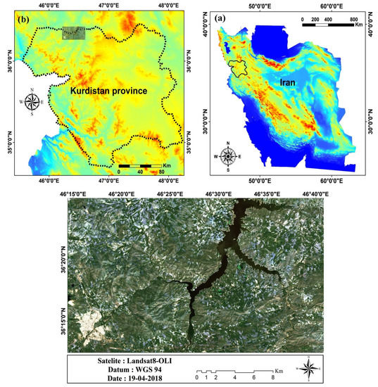
Figure 1.
Location of the study area in (a) Iran and (b) Kurdistan province.
3. Material and Methods
3.1. Data Acquisition and Pre-Processing
3.1.1. Sentinel-2B
Data from Sentinel-2B satellite image freely downloaded from the Copernicus Scientific Data Hub website (https://sentinels.copernicus.eu/web/sentinel/user-guides/sentinel-2-msi, accessed date: 18 February 2021) were used. Four tiles of Sentinel-2B cover the whole study area. Table 1 presents the details of data acquired. Two Sentinel 2A and 2B satellites were launched by the European Space Agency on 23 June 2015 and 7 March 2017, respectively. Both satellites are in the same orbit and have the same characteristics. Table 2 shows the spatial resolution of different bands based on wavelength. For pre-processing of Sentinel-2 B, first of all, visual image analysis was done to confirm the agreement of the georeferenced images. In the following, Sen2Cor tool, which is available in the Sentinel Application Platform (SNAP) software, was used for atmospheric correction. Then, we combined layer stacked image bands of 2, 3, 4, 8 into one file and image bands of 11 and 12, 20 m were added to a 10 m layer stack. Then, a 20 m resolution with layer stack was created to define the wavelength for each band in order to indicate relative abundance of features of interest, spectral indices (combinations of surface reflectance at two or more spectral bands).

Table 1.
List of the selected Sentinel-2B and Landsat-8 images for the study area.
Table 2.
Spectral bands of the Sentinel-2 B and Landsat-8 OLI satellite imagery.
3.1.2. Landsat-8
Data from Landsat-8 satellite image is open and freely available on the USGS website (https://glovis.usgs.gov/, accessed date: 18 February 2021). The whole area was covered by one tile for Landsat 8 on June 2018 (Table 3). As shown in Table 2, the OLI sensor has nine bands and is co-registered with the TIRS (Thermal Infrared Sensor) sensor, which has two spectral bands. The ground sampling distance for OLI and TIRS is 30 and 100 m, respectively. Unfortunately, the 12 μm TIRS band (band 11) has been remarkably affected by stray light, which compromises its utility for split-window atmospheric correction [44].
Table 3.
List of the selected the Landsat-8 operational Land Imager (OLI) images for the study area.
The pre-processing steps for the Landsat-8 involve radiometric calibration, top of the atmosphere reflectance and surface reflectance. In the first step, we broke Landsat 8 data into subsets as we did for the Sentinel-2 dataset. Then, Digital Number (DN) for each pixel was converted to radiance values using radiometric calibration. Removing the influence of the atmosphere is a necessary step to reach surface reflectance values. To do so, ENVI V5.3 software was used. This program offers various methods for atmospheric correction such as Dark Subtraction, FLAASH, Empirical Line, and Flat Field. In this work, we applied the Dark Object Subtraction (DOS) on the calibrated image to extract surface reflectance values. DOS works by searching each band to identify dark pixels. For this purpose, it is assumed that a dark object does not reflect any light and that any value greater than zero is the result of atmospheric scattering. Subtracting this value for each pixel from each band, scattering is then removed [45]. After atmospheric correction, the values of pixels show the surface reflectance. The methodology of this research is presented as a flowchart in Figure 2.
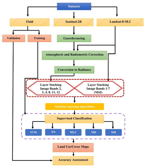
Figure 2.
Flowchart in this study.
3.2. Classification Training and Testing Data
We identified training and testing datasets that represent different surface cover types based on previously known actual surface cover types. These cover types were selected by field surveys in each land covers such as irrigated land, dry farming, range land (pasture), bare land, residential, and waterbodies. These areas were detected based on different supervised machine learning classification methods. We made sure that the training set had a sufficient number of independent samples for each class to exhibit the interclass variability [46]. After this, we used these specifically categorized training areas to recognize similar areas for each class using statistical algorithms. We used GPS (global positioning system) and high-resolution orthorectified Google Earth imagery as a reference for the selection and quality control of the training and testing samples with 2086 randomly selected ground truth points with a combination of 70%/30% (Table 4). The ground truth points used in this study is shown in Table S1 as Supplementary Materials.
Table 4.
The training and testing samples for land use/cover units.
3.3. Background of Image Classification Methods
3.3.1. Support Vector Machine Algorithm
The Support Vector Machine (SVM) model is a high-performing supervised machine learning technique that employs a binary classifier based on optimal separating hyper-plane and statistical machine learning theory [47]. The purpose of the optimal classification hyperplane is to distinguish between the two classes of used samples (the presence and absence classes) appropriately for a maximum of the classification margin in a feature space.
In general, the typical SVM model is separated into the two-class and multi-class SVM (combing a chain of two-class SVM). The two-class SVM is the most frequently applied machine learning model [48,49]. During the process of SVM, the separating hyperplane (H) is the probable planes for separating the two classes. SVM can find an optimal hyperplane by distinguishing the classes using the following equation [47]:
Subjected to the constraints as below:
where, w, b, , and c (>0) signifies a coefficient vector, the offset of the hyperplane from the beginning, the positive slack variable, and the penalty parameters of the errors, respectively. The details of two-class SVM can be referred in studies [50,51,52].
3.3.2. Artificial Neural Network Algorithm
Artificial Neural Network (ANN), which is based on the human biological neural network, is a nonlinear modeling tool that solves problems without any assumptions. Therefore, it has capability to identify complex relationships between input data types. This method has been widely used in different fields, such as landslide susceptibility mapping (LSM), landslide detection, classification, etc. [53,54,55]. The general structure of this method consists of three different layers. The first layer involves receiving data. In the second layer, which is also known as the hidden layer, the necessary calculations are applied to the data. These calculations are based on processing units called neurons. The number of neurons is obtained by the user based on a trial-and-error process. The last layer also specifies the final outputs. The network training structure of this method is such that the training samples enter the network through the input layer and then enter the middle layer after multiplying by the connecting weights of neurons. In the middle layer, the neurons also perform the necessary calculations and then send the resulting values to the output layer. Weights and biases are determined by means of a non-linear optimization procedure (training) that aims at minimizing a learning function conveying closeness between the observation and the ANN output.
Let signify n input neurons, while is output neurons. For the classification, the activation function applied in hidden neurons is expressed as below:
where are the connected weights between input neurons and output neurons and v and are the bias.
In this process, the number of nodes on the hidden layers used in ANN Algorithm is exactly equal to the number of bands. In addition, the training algorithm used to adjust weights and minimize the value of a loos function was gradient descent [56]. Furthermore, number of output neurons is the same as the number of the classes of land use map classes of the study area.
3.3.3. Maximum Likelihood Classification
Maximum likelihood classification is one of the most well-known and widely used classification algorithms in remote sensing, which is considered as a basic pixel method [35]. In this method, a pixel is assigned to the class that has the maximum likelihood (maximum probability) to it. This method relies on the assumption that the data of each class from each band has a normal distribution [35]. Therefore, selecting a few pixels is sufficient to provide an accurate estimate of the mean vector and the variance–covariance matrix. Moreover, as many samples as possible should be used so that the algorithm can take into account the many changes in spectral features. In general, two features of mean vector and covariance matrix are estimated for each pixel in order to calculate the similarity of each pixel with the considered classes. Bayesian law is used to calculate this likelihood as follows [45]:
where D (weighted distance) indicates the likelihood, c represents the specified class, X is the measurement vector of the desired pixel, Mc is the mean vector of the class c, and COVc represents the covariance matrix of the pixels of the class c.
3.3.4. Minimum Distance
The minimum distance classification method is based on calculating the mean vector of each class and the distance of unknown pixels to these mean vectors. In other words, the class whose mean values have the minimum distance to the desired pixel is assigned to the pixel. This method is a part of the supervised classification. Of the advantages of this method that have made it popular are its simple mathematics and the need for mean vector for each band of the training data [57]. Due to its simple logic, it does not require complex calculations and therefore has a good speed. It should also be considered that this method is not suitable in places where spectral classes are very close to each other, according to the following equation [58]
where Dist (distance) represents the distance of mean score to the unknown pixel), is the mean vector of the class c in the band k, and is the mean vector of the class c in the band I.
3.3.5. Mahalanobis Algorithm
The Mahalanobis algorithm (MH) proposed by Mahalanobis [59] originally relates to a distance measure that combines the correlation among the features MH relates to a generalized Euclidean Distance (ED) by means of the inverse of a variance-covariance matrix. In classification, the correlation among the image data plays an important role. It has been observed that MH provides greater accuracy than ED [60,61] where MH is used to measure the difference between the inverse similarity and dissimilarity matrices. It can be described by following equation:
where Ci means the covariance matrix for the particular imagined movement considered and T represents the transposition operator. The mean vector m stands for the average of the x vectors calculated.
3.4. Parameter Tuning
Parameter tuning has an effect role in the performance of the machine learning results [62]. Each machine learning algorithm has different tuning stages and tuned parameters [2]. An advanced machine learning algorithm features different tuning parameters. Setting the tuning parameters is one of the key phases of classification to improve the accuracy [43]. Hence, this study used different series of kernel function and penalty parameters for non-parametric classification in SVM. For the non-parametric classification of ANN, it used different hidden layers in order to select the most appropriate tuning parameters for producing the most accurate map. We in this study, tested a series of values for each parameters of the algorithms to obtain the optimal parameters resulted in highest overall classification accuracy. Then, we used of the overall accuracy and kappa index to compare the performance of classifiers [42]. We listed the parameters and the optimal values for each algorithm in Table 5 and Table 6.
Table 5.
Parameter tuning in Support Vector Machine (SVM) model in the LANDSAT and SENTINEL-2 images.
Table 6.
Parameter tuning in Artificial Neural Network (ANN) model in the LANDSAT and SENTINEL-2 images.
3.5. Classification Accuracy Scheme
Our classification scheme included six classes: irrigated land, dry farming, range land (pasture), bare land, residential area, and waterbodies (Table 7). In the study area, irrigated lands are not cultivated only be wheat but other strategic crops such as potato, sugar beet, and alfalfa. Therefore, we have to separate these land cover units. For example, Du et al. [63], Aslami and Ghorbani [64], Kingwell-Banham [65], Dobrinić et al. [66], and Eskandari et al. [67] have also been separated the irrigated lands from dry farming lands. The supervised classification was performed using SVM, ANN, MLC, MD, and Mahalanobis. We used of accuracy and kappa index to check and compare the performance of the algorithms in ability to classify the land cover/use units. Overall accuracy (OA) and kappa index can be computed based on the following equations:
where Dii is the number of observations in row i and column i of the confusion matrix, n is the number of rows in the error matrix, N is total number of counts in the confusion matrix, xi+ is the marginal total of row i, and x + i is the marginal total of column i.
4. Results and Analysis
4.1. Accuracy Assessment
Table 7 and Table 8 list the accuracy for SVM, ANN, MLC, MD, and MH for Sentinel 2 and Landsat 8, respectively. In many cases, the tuning parameters show identical Kappa coefficients, while their overall accuracies slightly vary. Thus, for a more accurate comparison, selecting the optimal tuning parameter, and producing the most accurate map, we used the overall accuracy as assessment criterion (Table 7 and Table 8). It is noted that the value in each class column mean of these tables is producer’s accuracy.
Table 7.
Accuracy and kappa measures of Sentinel 2.
Table 8.
Accuracy and kappa measures of Landsat 8-OLI.
4.2. Comparisons the Classifiers and Tuning Parameters
Our validation results indicated that, in general, SVM offered better accuracy in producing LULC maps for both sets of satellite data. Figure 3 illustrates the overall accuracy of the algorithms and the comparison between them for Sentinel 2 and Landsat 8 images. According to overall accuracy and the optimal tuning parameter, SVM algorithm performed best with overall accuracies of 95.82% and 94.78% for Sentinel 2 and Landsat 8, respectively (with Kappa coefficients 0.94 and 0.93) (Table 7). Figure 3 also shows the different results from other classification algorithms.
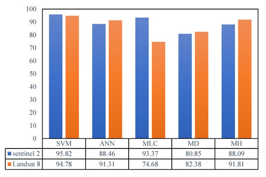
Figure 3.
Overall accuracy for each algorithm with optimal tuning parameters.
For Sentinel 2 data, after SVM, MLC ranked second with the overall accuracy of 93.37%. Further, ANN (with optimal parameters), MH, and MD algorithms ranked next with respective accuracies of 88.46%, 88.09%, and 80.85% and MD performing the poorest.
For Landsat 8 data, (Table 7; Figure 3), the MH classifier yielded the highest overall accuracy of 91.81%, and the Kappa coefficient of 0.89 had the second-best performance after SVM for generating LULC maps ta. This was followed by ANN (with optimal tuning parameters), MD, and MLC algorithms with respective overall accuracies of 91.31%, 82.38%, and 74.68%. Based on the results, MLC had the weakest performance (Kappa coefficient = 0.68).
In another comparison, different tuning parameters for non-parametric classifiers of SVM and ANN were used to determine the effect of optimal parameter tuning on the variation of classification results. For SVM, different values of kernel function and penalty parameter were tested. In this study, we compared four kernel types (linear, polynomial, sigmoid, and radial basis). Table 7 and Table 8 show how a linear kernel function offered the best classification accuracy for both Sentinel 2 (95.82% for SL150) and Landsat 8 (94.78% for SL200 and SL250). Comparing the results also indicated that the lowest accuracies belonged to radial kernel SR100 (overall accuracy of 93.86%) for Sentinel 2 image and SS100 sigmoid kernel (overall accuracy of 88.46%) for Landsat 8 image. For the penalty parameter, we tested values of 100, 150, 200, and 250. The optimal penalty parameter for the most accurate algorithm of Sentinel 2 data was 150 (SL 150), and these figures were 200 and 250 for Landsat 8 data (SL 200 and SL250). In addition, for the ANN classifier, we tested different numbers of hidden layers to clarify their effect on processing. As Table 7 and Table 8 show, running ANN with a single hidden layer offers the best performance for both datasets (88.46% for Sentinel 2 and 91.31% for Landsat 8). Further, the results show that increasing the hidden layers reduces algorithm accuracy. This reduction is such that three hidden layers result in accuracies of 18.89% and 9.3% for Sentinel 2 and Landsat 8, respectively.
4.3. Land Cover Change Assessment
To classify LULC maps, six classes (irrigated land, dry farming, range land (pasture), bare land, residential, and waterbodies) were used. Following the calculation of confusion matrix, we employed user accuracy to assess the differentiation of classes. Table 7 and Table 8 show these values for Sentinel 2 and Landsat 8 data. The higher the user accuracy, the higher the algorithm capability in spectrum differentiation for the respective class. First, we analyze Table 7, where the results indicate that with the optimal tuning parameter, the water body class has the highest error-free accuracy (100) for all algorithms. This is followed by MLC algorithm with the differentiation accuracy of 99.64 for the irrigated land class. For the classes dry farming, range land, bare land, and residential, SVM, MLC, ANN, and MLC offer the best classification accuracies, respectively (97.45, 91.55, 94.87, and 98.7). Based on the tuning parameters, SL100 and SL150 have the highest user accuracy for irrigated land class and the lowest accuracy belonged to ANN-H2 and ANN-H3 (Table 7).
Table 8 shows that similar to the case of Sentinel 2 data, with optimal tuning parameters the waterbody class in Landsat 8 image has the lowest classification error (100 for all algorithms save for MLC). For the irrigated land class, SVM algorithm (user accuracy= 98.2) offers the best performance, followed by classes: dry farming, pasture, bare land, and residential, where MH, MH, SVM, and MLC offer the best accuracy (97.85, 90, 96.1, 91.89). Among tuning parameters, SL100, SL150, SL200, SL250, SP150, SP200, SP250, SR150, and SR200 have the highest accuracy and ANN-H3 offers the worst performances. Figure 4 shows ANN RMSE curve under different iterations in Sentinel-2 and Landsat 8.
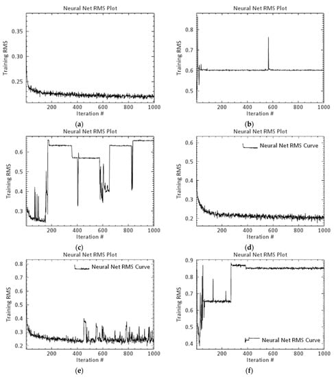
Figure 4.
Artificial Neural Network (ANN) Root Mean Square Error (RMSE) curve under different iterations in Sentinel-2: (a) hidden layer equal to 1, (b) hidden layer equal to 2, and (c) hidden layer equal to 3 and in Landsat 8: (d) hidden layer equal to 1, (e) hidden layer equal to 2, and (f) hidden layer equal to 3.
4.4. Land Cover Change Detection Map
Figure 5 illustrates the land cover differences that are identified within the study area by five SVM, ANN, MLC, MD, and MH machine learning methods for Sentinel and Landsat images. In the SVM method, the classification of the study area was done based on five kernel functions: Linear, Polynomial, Sigmoid, and Radial basis. The purpose of implementing these models was to estimate and compare the performance of models with various error levels (100, 150, and 200). Results indicated that all outputs in the SVM method show the highest degree of accuracy in identifying and distinguishing land use in the study area compared to other methods for both Sentinel and Landsat images.
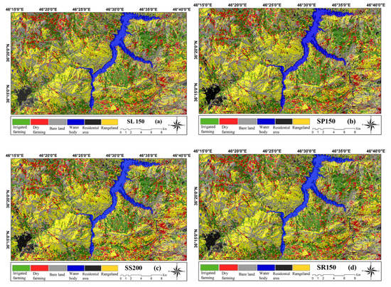
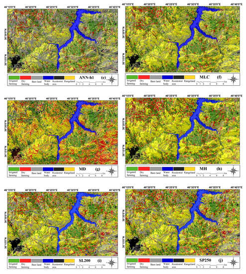
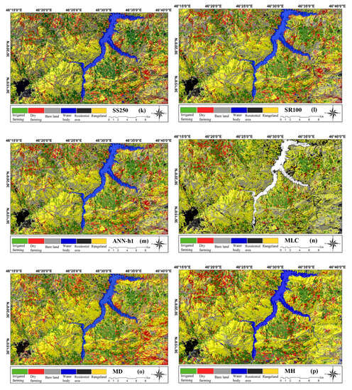
Figure 5.
Land cover change maps by sentinel-2: (a) SL150, (b) SP150, (c) SS200, (d) SR150, (e) ANN-H1, (f) MLC, (g) MD, and (h) Mh and landsat-8: (i) SL 200, (j) SP250, (k) SS250, (l) SR100, (m) ANN-H1, (n) MLC, (o) MD, and (p) MH.
The LULC map of the ANN-H1 model in the Sentinel image shows a larger area of bare land, which does not correspond to reality. The land cover change map of the ANN-H2 model does not have the ability to identify the blue class (water bodies) and shows a larger area of the range as bare land. However, the ANN-H3 model was not able to identify any of the six classification classes and shows the lowest accuracy according to the Table 5. The land cover change map prepared by the ANN-H1 model based on the Landsat image depicted land classification with a high degree of accuracy (91.3). However, the land cover change map by the ANN-H2 model performed very poorly in identifying the irrigated areas. Moreover, the output of ANN-H3 in the Landsat image did not show any of the six classification classes.
The MLC method for the Sentinel images, except for a percentage of error in showing the dry-farming class, performed poorly and showed a higher percentage of the study area as rangeland unit (93.37). The MLC method did not identify waterbodies by Landsat images and exaggerated the identification of the residential areas (74.68). The LULC map obtained by the MD method based on both Sentinel and Landsat images, and especially by the Sentinel images to detect the dry-farming class, is associated with a very high level of exaggeration and accuracy of 80.85 and 82.38, respectively. Finally, the classification in the MH method was not as good as the MD model and showed the highest level as the rangeland class.
5. Discussion
In this study, we used the same algorithm processing condition (with identical training and validation dataset), to compare Sentinel 2 and Landsat 8 data for optimal LULC mapping. First, we compared the algorithms based on optimal tuning parameters for SVM and ANN. The resulting overall accuracy and Kappa coefficient showed that the non-parametric SVM algorithm offers the best classification for both satellite datasets. Nevertheless, Sentinel 2 had a slightly higher accuracy compared to the Landsat 8 OLI sensor. Comparison with other algorithms confirms the effect of input data on the end results. For example, the MLC classifier for Sentinel 2 ranks second in accuracy after SVM; whereas, for Landsat 8 data, it has the poorest performance of all. Likewise, the overall accuracy of MH algorithm for Sentinel 2 is lower than those for Landsat 8 as the second-best accuracy after SVM. The observation implies that we cannot be certain about the choice of an algorithm until we have compared its performance with similar methods, therefore, simultaneous execution of several methods and comparing their results produces the most accurate map.
In the second step, we focused on the effect of tuning parameters on SVM and ANN classifiers. SVM results showed that for both Sentinel 2 and Landsat 8, the linear kernel offers the optimal output. Here, respective penalty parameters of 150 and 200 were used for sentinel 2 and Landsat. For Sentinel 2 images, a radial kernel with the penalty parameter 100 had the lowest accuracy, while for Landsat 8, the sigmoid kernel with the penalty parameter 100 had a lower classification accuracy. The comparisons show the effect of tuning parameters on the results, implying that testing different values is critical to producing a quality map, as optimizing the tuning parameters increases the accuracy and reduces classification error. Moreover, we used different numbers of hidden layers in ANN to find the effect of increasing them on the processing and the results. Both datasets experienced reduced overall accuracy and Kappa coefficient by increasing the number of hidden layers. Thus, the output analysis revealed that a more complex network structure does not necessarily mean a more optimal result while forcing the software to increase processing time.
In the last step, we estimated the accuracy of each algorithm in map classification. Our investigations showed that with optimal tuning parameters, all algorithms differentiate the water body with 100% accuracy. After that, MLC algorithm performed best for Sentinel 2 data while SVM performed best for Landsat 8 data in detecting the irrigated land class. Another comparison showed that in both satellite data, the parametric algorithm MLC had the most accurate classification for residential zones. This outcome is significant when put against more advanced classification methods (e.g., SVM and ANN) because due to the high spectrum similarity of residential regions with other terrain features such as bare land, their differentiation is one of the most challenging parts of processing. Comparisons illustrate that although more advanced machine learning methods such as SVM offer more accurate image classification in the presence of different classes, an algorithm such as MLC performs better when attempting to classify images in special spectrums such as residential terrains. In addition, the classes “irrigated land,” “dry farming,” and “range land (pasture)” have high spectrum similarity, which makes their differentiation difficult. The results also indicated that for Sentinel 2 data, MLC algorithm offers the best accuracy in differentiating the spectrums of “irrigated land” and “pasture” classes while SVM performed best for “dry farming.” For Landsat 8 data, SVM for “irrigated land” and MH algorithm for “dry farming” and “pasture” offer the highest accuracy in differentiating classes. The MLC and MD frequently used classification also were compared. The overall accuracy shows that the MLC algorithm has better performance than the MD for Sentinel-2 data, and MD provides better accuracy than MLC for LANDSAT8 data. The results display that although an advanced supervised algorithm such as SVM can have more overall accuracy for a class, it may perform weaker than a simpler method such as MLC in detecting and differentiating the spectrum of a specific class in LULC map. The ANN results show that increasing the hidden layers does not necessarily increase classification accuracy and may even work against it. It is essential to compare the results with those of similar studies, because it both offers a more realistic view of the methods and helps develop the future studies. There are numerous studies on classification via supervised algorithms, some of which are the following.
Adam et al. [21] used two machine learning algorithms (SVM and RF) to generate the LULC of a region on the east African coast. First, they obtained a high-resolution RapidEye image of the zone and then performed the required pre-processing. After that, they used training data and advanced methods (SVM and RF) to classify the region into 11 classes. Then, they generated the classification maps and compared them based on overall accuracy, Kappa coefficient, and McNamer’s test. They found that RF algorithm (overall accuracy = 93.07%) is more accurate compared to SVM (overall accuracy = 91.80%). Further, the Kappa coefficient for both methods was 0.92 Kumar et al. [68] used three algorithms (SVM, ANN, and SAM) to classify the produce of Varanasi in India. They first created a database consisting of training and validation data and the LISS IV sensor data. Then, they divided the zone to 13 classes and compared the results based on overall accuracies. They found that SVM and ANN with overall accuracies above 90% performed better than SAM. Further, SVM model with the accuracy of 93.45% performed better in classifying the studied zone compared to ANN model with the accuracy of 92.32%. Our study obtained similar results with lower resolution imagery. Based on overall accuracy, SVM algorithm performed better than ANN for the data of Sentinel 2 and Landsat 8 with respective differences of 7.36% and 3.47%. In another study, Jia et al. [69] attempted to classify land cover in Beijing, China, by comparing the images of Landsat 7 and Landsat 8 and using supervised algorithms MLC and SVM. They found that the SVM algorithm with an overall accuracy of 91.03% and the Kappa coefficient of 0.89 is more accurate compared to the MLC algorithm with the overall accuracy of 90.4% and the Kappa coefficient of 0.88. Further, they found that the quality of input data affects the end results, as OLI data performed better than ETM+ data. The results of the current study also indicate that SVM performs better than MLC with a difference of 2.45% for Sentinel 2 data and a noticeable difference of 21.1% for Landsat 8 data. Noi et al. [2] compared the results of three algorithms (RF, KNN, and SVM) to classify the Sentinel 2 data in a region of Vietnam. To show the impact of training pixels on the accuracy of the output map, they divided the training dataset into 14 sizes. The results showed that of the three algorithms, SVM offers a higher mean overall accuracy and performs better in producing the LULC maps, followed by RF and KNN algorithms by the order of their performance. Talukdar et al. [25] used six machine learning algorithms (RF, SVM, ANN, Fuzzy ARTMAP, SAM, and MD) to classify the LULC of three different regions alongside the Ganga River. For this purpose, first they obtained the input data consisting of the Landsat 8 image, training dataset, and validation dataset and then used the said algorithms to classify the regions. Ultimately, they used Kappa coefficient, AUC, and RMSE to compare the results. They found that RF algorithm (Kappa coefficient = 0.89, AUC = 0.91) performs slightly better than ANN in classifying the studied region, while MD algorithm (Kappa coefficient = 0.82 and AUC = 0.83) was the least accurate. In another study, Rahman et al. [59] applied three algorithms (RF, SVM, and their combination) to classify LULC in the rural (Bhola) and urban (Dhaka) regions using Landsat-8, Sentinel-2, and Planet satellite images. Their results showed that Sentinel-2 has better results among the three images. Further, they found that the SVM performs best with an overall accuracy (0.969 and 0.983) and kappa values (0.948 and 0.968) compared to RF and stack algorithms. Keshtkar et al. [60] compared random forest (RF), decision tree (DT), and support vector machine (SVM) in pixel-based and object-based approaches to classify land cover change from 1990 to 2010 using Landsat-8 image. They concluded that the object-based SVM classifier has a better performance than RF and DT (overall accuracy = 93.54% and kappa value = 0.88). Their results indicated that the expansion of built-up areas (with an annual increase in 4.53%) caused the most significant change (with a yearly decrease in about 0.81% in natural lands). Tu et al. [61] attempted to improve 10 m resolution land cover classification with different images (Sentinel-1, Sentinel-2, and Luojia-1) and machine learning algorithms in Guangdong province, China. They found that the RF model performs best results with overall accuracy and kappa coefficient of 86.12% and 0.84, respectively, compared to other CART, MD, and SVM models.
The results of this study are in line with those of previous studies. The evaluations illustrate that the SVM algorithm yields higher overall accuracy compared to other supervised algorithms. Our data comparison revealed that while using identical training and validation datasets, the satellite image effects the end results and is therefore one of the key steps in producing LULC maps. Further, proper tuning parameters increase map accuracy. The data type and processing used in the study can help local planners and authorities with producing more accurate maps.
6. Conclusions
The current study evaluated and then compared five supervised classification algorithms for generating LULC maps. To factor the effect of input data, two images from Sentinel 2 (with resolution of 20 m) and Landsat 8 (with resolution 30 m) were used. Different tuning parameters were applied for SVM and ANN algorithms in order to determine their effect on classification accuracy. With optimal tuning parameters, evaluating the overall accuracy indicated that among the utilized classification methods, SVM performed best in classifying the studied region for both images; however, Sentinel 2 data performed slightly better in class differentiation, although this superiority was not identical for all algorithms. ANN, MD, and MH algorithms on Landsat 8 data indicated higher accuracy compared to Sentinel 2 data. Another key finding was the effect of different tuning parameters on classification accuracy. SVM classification with linear kernel function proved more accurate in classifying both images. For Sentinel 2 penalty parameter 150 and for Landsat 8 penalty parameters 150 and 200 performed the best in training SVM. Further, for Sentinel 2 and Landsat 8, respectively, radial kernel and sigmoid kernel had given the lowest accuracies. Comparing the hidden layers of the ANN classifier, the best output was given by a single hidden layer and increasing these layers not only increased processing time but also greatly reduced accuracy. Further, considering the user accuracy, the classification performance of each algorithm in class differentiation was evaluated. For the “waterbody” class, all algorithms offered an accuracy of 100%. Although the overall classification accuracy of SVM was higher, analyzing the results indicated that for both satellite data, the MLC algorithm was more accurate in classifying residential regions. For the classes “irrigated land,” “dry farming,” “range land (pasture),” and “bare land,” for Sentinel 2 data, the MLC, SVM, MLC, and ANN algorithms, respectively, offered the best accuracies, while for Landsat 8 data SVM, MH, MH, and SVM algorithms were the most accurate. The results also indicated that different satellite data influenced the processing due to different resolutions and electromagnetic spectrum bands, changing the classification accuracy of each algorithm.
Supplementary Materials
The following are available online at https://www.mdpi.com/article/10.3390/rs13071349/s1, Table S1: The ground truth points used in this study.
Author Contributions
L.G., A.N., S.P., H.S., A.S., W.C., N.A.-A., M.G. (Marten Geertsema), M.P.A., M.G. (Mehdi Gholamnia), J.D. and A.A. contributed equally to the work. L.G., H.S., A.S. and M.P.A. collected field data and conducted the land cover/use classification and analysis. L.G., A.N., S.P., H.S., A.S., M.P.A. and J.D. wrote the manuscript. W.C., N.A.-A., M.G. (Marten Geertsema), M.G. (Mehdi Gholamnia) and A.A. provided critical comments in planning this paper and edited the manuscript. All the authors discussed the results and edited the manuscript. All authors have read and agreed to the published version of the manuscript.
Funding
This research was supported by the University of Kurdistan, Iran, based on grant number GRC98-04469-1.
Conflicts of Interest
The authors declare no conflict of interest.
References
- Bevington, A.; Gleason, H.; Giroux-Bougard, X.; de Jong, J.T. A Review of Free Optical Satellite Imagery for Watershed-Scale Landscape Analysis. Conflu. J. Watershed Sci. Manag. 2018, 2. [Google Scholar] [CrossRef]
- Thanh Noi, P.; Kappas, M. Comparison of random forest, k-nearest neighbor, and support vector machine classifiers for land cover classification using Sentinel-2 imagery. Sensors 2018, 18, 18. [Google Scholar] [CrossRef]
- Yang, D.; Fu, C.-S.; Smith, A.C.; Yu, Q. Open land-use map: A regional land-use mapping strategy for incorporating OpenStreetMap with earth observations. Geo Spat. Inf. Sci. 2017, 20, 269–281. [Google Scholar] [CrossRef]
- Tien Bui, D.; Shahabi, H.; Mohammadi, A.; Bin Ahmad, B.; Bin Jamal, M.; Ahmad, A. Land cover change mapping using a combination of Sentinel-1 data and multispectral satellite imagery: A case study of Sanandaj county, Kurdistan, Iran. Appl. Ecol. Environ. Res. 2019, 17, 5449–5463. [Google Scholar] [CrossRef]
- Wulder, M.A.; Coops, N.C.; Roy, D.P.; White, J.C.; Hermosilla, T. Land cover 2.0. Int. J. Remote Sens. 2018, 39, 4254–4284. [Google Scholar] [CrossRef]
- Topaloğlu, R.H.; Sertel, E.; Musaoğlu, N. Assessment of classification accuracies of Sentinel-2 and Landsat-8 data for land cover/use mapping. Int. Arch. Photogramm. Remote Sens. Spat. Inf. Sci. 2016, 41, 1055–1059. [Google Scholar] [CrossRef]
- Shahabi, H.; Ahmad, B.B.; Mokhtari, M.H.; Zadeh, M.A. Detection of urban irregular development and green space destruction using normalized difference vegetation index (NDVI), principal component analysis (PCA) and post classification methods: A case study of Saqqez city. Int. J. Phys. Sci. 2012, 7, 2587–2595. [Google Scholar]
- Shahabi, H.; Shirzadi, A.; Ghaderi, K.; Omidvar, E.; Al-Ansari, N.; Clague, J.J.; Geertsema, M.; Khosravi, K.; Amini, A.; Bahrami, S. Flood detection and susceptibility mapping using sentinel-1 remote sensing data and a machine learning approach: Hybrid intelligence of bagging ensemble based on k-nearest neighbor classifier. Remote Sens. 2020, 12, 266. [Google Scholar] [CrossRef]
- Halder, A.; Ghosh, A.; Ghosh, S. Supervised and unsupervised landuse map generation from remotely sensed images using ant based systems. Appl. Soft Comput. 2011, 11, 5770–5781. [Google Scholar] [CrossRef]
- Sathya, P.; Malathi, L. Classification and segmentation in satellite imagery using back propagation algorithm of ann and k-means algorithm. Int. J. Mach. Learn. Comput. 2011, 1, 422. [Google Scholar] [CrossRef]
- Al-Doski, J.; Mansorl, S.B.; Shafri, H.Z.M. Image classification in remote sensing. J. Environ. Earth Sci. 2013, 3, 10. [Google Scholar]
- Rozenstein, O.; Karnieli, A. Comparison of methods for land-use classification incorporating remote sensing and GIS inputs. Appl. Geogr. 2011, 31, 533–544. [Google Scholar] [CrossRef]
- Yousefi, S.; Mirzaee, S.; Tazeh, M.; Pourghasemi, H.; Karimi, H. Comparison of different algorithms for land use mapping in dry climate using satellite images: A case study of the Central regions of Iran. Desert 2015, 20, 1–10. [Google Scholar]
- Al-Ahmadi, F.; Hames, A. Comparison of four classification methods to extract land use and land cover from raw satellite images for some remote arid areas, Kingdom of Saudi Arabia. Earth 2009, 20, 167–191. [Google Scholar] [CrossRef]
- Bett, S.K.; Palamuleni, L.G.; Ruhiiga, T.M. Monitoring of urban sprawl using minimum distance supervised classification algorithm in Rustenburg, South Africa. Asia Life Sci. 2013, 9, 245–261. [Google Scholar]
- Kantakumar, L.N.; Neelamsetti, P. Multi-temporal land use classification using hybrid approach. Egypt. J. Remote Sens. Space Sci. 2015, 18, 289–295. [Google Scholar] [CrossRef]
- Rijal, S.; Rimal, B.; Sloan, S. Flood hazard mapping of a rapidly urbanizing city in the foothills (Birendranagar, Surkhet) of Nepal. Land 2018, 7, 60. [Google Scholar] [CrossRef]
- Rimal, B.; Rijal, S.; Kunwar, R. Comparing Support Vector Machines and Maximum Likelihood Classifiers for Mapping of Urbanization. J. Indian Soc. Remote Sens. 2020, 48, 71–79. [Google Scholar] [CrossRef]
- Omer, G.; Mutanga, O.; Abdel-Rahman, E.M.; Adam, E. Performance of support vector machines and artificial neural network for mapping endangered tree species using WorldView-2 data in Dukuduku forest, South Africa. IEEE J. Sel. Top. Appl. Earth Obs. Remote Sens. 2015, 8, 4825–4840. [Google Scholar] [CrossRef]
- Zhang, C.; Sargent, I.; Pan, X.; Li, H.; Gardiner, A.; Hare, J.; Atkinson, P.M. An object-based convolutional neural network (OCNN) for urban land use classification. Remote Sens. Environ. 2018, 216, 57–70. [Google Scholar] [CrossRef]
- Adam, E.; Mutanga, O.; Odindi, J.; Abdel-Rahman, E.M. Land-use/cover classification in a heterogeneous coastal landscape using RapidEye imagery: Evaluating the performance of random forest and support vector machines classifiers. Int. J. Remote Sens. 2014, 35, 3440–3458. [Google Scholar] [CrossRef]
- Eisavi, V.; Homayouni, S.; Yazdi, A.M.; Alimohammadi, A. Land cover mapping based on random forest classification of multitemporal spectral and thermal images. Environ. Monit. Assess. 2015, 187, 291. [Google Scholar] [CrossRef]
- Teluguntla, P.; Thenkabail, P.S.; Oliphant, A.; Xiong, J.; Gumma, M.K.; Congalton, R.G.; Yadav, K.; Huete, A. A 30-m landsat-derived cropland extent product of Australia and China using random forest machine learning algorithm on Google Earth Engine cloud computing platform. ISPRS J. Photogramm. Remote Sens. 2018, 144, 325–340. [Google Scholar] [CrossRef]
- Martins, S.; Bernardo, N.; Ogashawara, I.; Alcantara, E. Support vector machine algorithm optimal parameterization for change detection mapping in Funil Hydroelectric Reservoir (Rio de Janeiro State, Brazil). Modeling Earth Syst. Environ. 2016, 2, 138. [Google Scholar] [CrossRef]
- Talukdar, S.; Singha, P.; Mahato, S.; Pal, S.; Liou, Y.-A.; Rahman, A. Land-Use Land-Cover Classification by Machine Learning Classifiers for Satellite Observations—A Review. Remote Sens. 2020, 12, 1135. [Google Scholar] [CrossRef]
- Bahadur, K. Improving Landsat and IRS image classification: Evaluation of unsupervised and supervised classification through band ratios and DEM in a mountainous landscape in Nepal. Remote Sens. 2009, 1, 1257–1272. [Google Scholar] [CrossRef]
- Boori, M.; Paringer, R.; Choudhary, K.; Kupriyanov, A. Supervised and unsupervised classification for obtaining land use/cover classes from hyperspectral and multi-spectral imagery. In Proceedings of the Sixth International Conference on Remote Sensing and Geoinformation of the Environment (RSCy2018), Paphos, Cyprus, 26–29 March 2018; p. 107730L. [Google Scholar]
- Duro, D.C.; Franklin, S.E.; Dubé, M.G. A comparison of pixel-based and object-based image analysis with selected machine learning algorithms for the classification of agricultural landscapes using SPOT-5 HRG imagery. Remote Sens. Environ. 2012, 118, 259–272. [Google Scholar] [CrossRef]
- Ma, L.; Li, M.; Ma, X.; Cheng, L.; Du, P.; Liu, Y. A review of supervised object-based land-cover image classification. ISPRS J. Photogramm. Remote Sens. 2017, 130, 277–293. [Google Scholar] [CrossRef]
- Shafizadeh-Moghadam, H.; Valavi, R.; Shahabi, H.; Chapi, K.; Shirzadi, A. Novel forecasting approaches using combination of machine learning and statistical models for flood susceptibility mapping. J. Environ. Manag. 2018, 217, 1–11. [Google Scholar] [CrossRef]
- Mosavi, A.; Shirzadi, A.; Choubin, B.; Taromideh, F.; Hosseini, F.S.; Borji, M.; Shahabi, H.; Salvati, A.; Dineva, A.A. Towards an Ensemble Machine Learning Model of Random Subspace Based Functional Tree Classifier for Snow Avalanche Susceptibility Mapping. IEEE Access 2020, 8, 145968–145983. [Google Scholar] [CrossRef]
- Tien Bui, D.; Shahabi, H.; Shirzadi, A.; Chapi, K.; Alizadeh, M.; Chen, W.; Mohammadi, A.; Ahmad, B.; Panahi, M.; Hong, H. Landslide Detection and Susceptibility Mapping by AIRSAR Data Using Support Vector Machine and Index of Entropy Models in Cameron Highlands, Malaysia. Remote Sens. 2018, 10, 1527. [Google Scholar] [CrossRef]
- Nhu, V.-H.; Mohammadi, A.; Shahabi, H.; Ahmad, B.B.; Al-Ansari, N.; Shirzadi, A.; Clague, J.J.; Jaafari, A.; Chen, W.; Nguyen, H. Landslide susceptibility mapping using machine learning algorithms and remote sensing data in a tropical environment. Int. J. Environ. Res. Public Health 2020, 17, 4933. [Google Scholar] [CrossRef]
- Mohammadi, A.; Baharin, B.; Shahabi, H. Land cover mapping using a novel combination model of satellite imageries: Case study of a part of the Cameron Highlands, Pahang, Malaysia. Appl. Ecol. Environ. Res. 2019, 17, 1835–1848. [Google Scholar] [CrossRef]
- Mondal, A.; Kundu, S.; Chandniha, S.K.; Shukla, R.; Mishra, P. Comparison of support vector machine and maximum likelihood classification technique using satellite imagery. Int. J. Remote Sens. GIS 2012, 1, 116–123. [Google Scholar]
- Ghosh, A.; Joshi, P.K. A comparison of selected classification algorithms for mapping bamboo patches in lower Gangetic plains using very high resolution WorldView 2 imagery. Int. J. Appl. Earth Obs. Geoinf. 2014, 26, 298–311. [Google Scholar] [CrossRef]
- Gopinath, G.; Sasidharan, N.; Surendran, U. Landuse classification of hyperspectral data by spectral angle mapper and support vector machine in humid tropical region of India. Earth Sci. Inform. 2020, 13, 633–640. [Google Scholar] [CrossRef]
- Karan, S.K.; Samadder, S.R. A comparison of different land-use classification techniques for accurate monitoring of degraded coal-mining areas. Environ. Earth Sci. 2018, 77, 713. [Google Scholar] [CrossRef]
- Pouteau, R.; Collin, A.; Stoll, B. A Comparison of Machine Learning Algorithms for Classification of Tropical Ecosystems Observed by Multiple Sensors at Multiple Scales. Available online: http://pages.upf.pf/Benoit.Stoll/pdf/2011-isrse34-comparison.pdf (accessed on 18 February 2021).
- Heydari, S.S.; Mountrakis, G. Effect of classifier selection, reference sample size, reference class distribution and scene heterogeneity in per-pixel classification accuracy using 26 Landsat sites. Remote Sens. Environ. 2018, 204, 648–658. [Google Scholar] [CrossRef]
- Thakkar, A.; Desai, V.; Patel, A.; Potdar, M. Land use/land cover classification using remote sensing data and derived indices in a heterogeneous landscape of a khan-kali watershed, Gujarat. Asian J. Geoinformatics 2015, 14, 1–12. [Google Scholar]
- Qian, Y.; Zhou, W.; Yan, J.; Li, W.; Han, L. Comparing machine learning classifiers for object-based land cover classification using very high resolution imagery. Remote Sens. 2015, 7, 153–168. [Google Scholar] [CrossRef]
- Bagheri, M.; Akbari, A.; Mirbagheri, S.A. Advanced control of membrane fouling in filtration systems using artificial intelligence and machine learning techniques: A critical review. Process. Saf. Environ. Prot. 2019, 123, 229–252. [Google Scholar] [CrossRef]
- Montanaro, M.; Gerace, A.; Lunsford, A.; Reuter, D. Stray light artifacts in imagery from the Landsat 8 Thermal Infrared Sensor. Remote Sens. 2014, 6, 10435–10456. [Google Scholar] [CrossRef]
- Richards, J. Remote Sensing Digital Image Analysis; Springer: Berlin/Heidelberg, Germany, 1999; p. 240. [Google Scholar]
- Muñoz-Marí, J.; Bruzzone, L.; Camps-Valls, G. A support vector domain description approach to supervised classification of remote sensing images. IEEE Trans. Geosci. Remote Sens. 2007, 45, 2683–2692. [Google Scholar] [CrossRef]
- Vapnik, V. The support vector method of function estimation. In Nonlinear Modeling; Springer: Berlin/Heidelberg, Germany, 1998; pp. 55–85. [Google Scholar]
- Dou, J.; Paudel, U.; Oguchi, T.; Uchiyama, S.; Hayakavva, Y.S. Shallow and Deep-Seated Landslide Differentiation Using Support Vector Machines: A Case Study of the Chuetsu Area, Japan. Terr. Atmos. Ocean. Sci. 2015, 26, 227–239. [Google Scholar] [CrossRef]
- Yao, X.; Tham, L.G.; Dai, F.C. Landslide susceptibility mapping based on support vector machine: A case study on natural slopes of Hong Kong, China. Geomorphology 2008, 101, 572–582. [Google Scholar] [CrossRef]
- Tien Bui, D.; Shirzadi, A.; Shahabi, H.; Geertsema, M.; Omidvar, E.; Clague, J.J.; Thai Pham, B.; Dou, J.; Talebpour Asl, D.; Bin Ahmad, B. New ensemble models for shallow landslide susceptibility modeling in a semi-arid watershed. Forests 2019, 10, 743. [Google Scholar] [CrossRef]
- Mohammadi, A.; Shahabi, H.; Bin Ahmad, B. Land-Cover Change Detection in a Part of Cameron Highlands, Malaysia Using ETM+ Satellite Imagery and Support Vector Machine (SVM) Algorithm. Environ. Asia 2019, 12, 145–154. [Google Scholar]
- Hong, H.; Liu, J.; Zhu, A.-X.; Shahabi, H.; Pham, B.T.; Chen, W.; Pradhan, B.; Bui, D.T. A novel hybrid integration model using support vector machines and random subspace for weather-triggered landslide susceptibility assessment in the Wuning area (China). Environ. Earth Sci. 2017, 76, 652. [Google Scholar] [CrossRef]
- Nhu, V.-H.; Shirzadi, A.; Shahabi, H.; Singh, S.K.; Al-Ansari, N.; Clague, J.J.; Jaafari, A.; Chen, W.; Miraki, S.; Dou, J. Shallow Landslide Susceptibility Mapping: A Comparison between Logistic Model Tree, Logistic Regression, Naïve Bayes Tree, Artificial Neural Network, and Support Vector Machine Algorithms. Int. J. Environ. Res. Public Health 2020, 17, 2749. [Google Scholar] [CrossRef]
- Shirzadi, A.; Shahabi, H.; Chapi, K.; Bui, D.T.; Pham, B.T.; Shahedi, K.; Ahmad, B.B. A comparative study between popular statistical and machine learning methods for simulating volume of landslides. Catena 2017, 157, 213–226. [Google Scholar] [CrossRef]
- Chen, W.; Pourghasemi, H.R.; Zhao, Z. A GIS-based comparative study of Dempster-Shafer, logistic regression and artificial neural network models for landslide susceptibility mapping. Geocarto Int. 2017, 32, 367–385. [Google Scholar] [CrossRef]
- Srivastava, P.K.; Han, D.; Rico-Ramirez, M.A.; Bray, M.; Islam, T. Selection of classification techniques for land use/land cover change investigation. Adv. Space Res. 2012, 50, 1250–1265. [Google Scholar] [CrossRef]
- Bouaziz, M.; Eisold, S.; Guermazi, E. Semiautomatic approach for land cover classification: A remote sensing study for arid climate in southeastern Tunisia. Euro Mediterr. J. Environ. Integr. 2017, 2, 24. [Google Scholar] [CrossRef]
- Mohamed, E.S.; Belal, A.; Shalaby, A. Impacts of soil sealing on potential agriculture in Egypt using remote sensing and GIS techniques. Eurasian Soil Sci. 2015, 48, 1159–1169. [Google Scholar] [CrossRef]
- Mahalanobis, P. Mahalanobis Distance. Proceedings National Institute of Science of India, New Delhi, India, June 1999; Indian Academy of Sciences: New Delhi, India, 1999; pp. 234–256. [Google Scholar]
- Mei, J.; Liu, M.; Wang, Y.-F.; Gao, H. Learning a mahalanobis distance-based dynamic time warping measure for multivariate time series classification. IEEE Trans. Cybern. 2015, 46, 1363–1374. [Google Scholar] [CrossRef]
- Prekopcsák, Z.; Lemire, D. Time series classification by class-specific Mahalanobis distance measures. Adv. Data Anal. Classif. 2012, 6, 185–200. [Google Scholar] [CrossRef]
- Shirzadi, A.; Asadi, S.; Shahabi, H.; Ronoud, S.; Clague, J.J.; Khosravi, K.; Pham, B.T.; Ahmad, B.B.; Bui, D.T. A novel ensemble learning based on Bayesian Belief Network coupled with an extreme learning machine for flash flood susceptibility mapping. Eng. Appl. Artif. Intell. 2020, 96, 103971. [Google Scholar] [CrossRef]
- Du, L.; Song, N.; Liu, K.; Hou, J.; Hu, Y.; Zhu, Y.; Wang, X.; Wang, L.; Guo, Y. Comparison of two simulation methods of the temperature vegetation dryness index (TVDI) for drought monitoring in semi-arid regions of China. Remote Sens. 2017, 9, 177. [Google Scholar] [CrossRef]
- Aslami, F.; Ghorbani, A. Object-based land-use/land-cover change detection using Landsat imagery: A case study of Ardabil, Namin, and Nir counties in northwest Iran. Environ. Monit. Assess. 2018, 190, 376. [Google Scholar] [CrossRef]
- Kingwell-Banham, E. Dry, rainfed or irrigated? Reevaluating the role and development of rice agriculture in Iron Age-Early Historic South India using archaeobotanical approaches. Archaeol. Anthropol. Sci. 2019, 11, 6485–6500. [Google Scholar] [CrossRef]
- Dobrinić, D.; Medak, D.; Gašparović, M. Integration of Multitemporal SENTINEL-1 and SENTINEL-2 Imagery for Land-Cover Classification Using Machine Learning Methods. Int. Arch. Photogramm. Remote Sens. Spat. Inf. Sci. 2020, 43, 91–98. [Google Scholar] [CrossRef]
- Eskandari, S.; Reza Jaafari, M.; Oliva, P.; Ghorbanzadeh, O.; Blaschke, T. Mapping land cover and tree canopy cover in Zagros forests of Iran: Application of Sentinel-2, Google Earth, and field data. Remote Sens. 2020, 12, 1912. [Google Scholar] [CrossRef]
- Kumar, P.; Gupta, D.K.; Mishra, V.N.; Prasad, R. Comparison of support vector machine, artificial neural network, and spectral angle mapper algorithms for crop classification using LISS IV data. Int. J. Remote Sens. 2015, 36, 1604–1617. [Google Scholar] [CrossRef]
- Jia, K.; Wei, X.; Gu, X.; Yao, Y.; Xie, X.; Li, B. Land cover classification using Landsat 8 operational land imager data in Beijing, China. Geocarto Int. 2014, 29, 941–951. [Google Scholar] [CrossRef]


Publisher’s Note: MDPI stays neutral with regard to jurisdictional claims in published maps and institutional affiliations. |
© 2021 by the authors. Licensee MDPI, Basel, Switzerland. This article is an open access article distributed under the terms and conditions of the Creative Commons Attribution (CC BY) license (https://creativecommons.org/licenses/by/4.0/).