Article

Evaluating the Detection of Mesoscale Outflow Boundaries Using Scatterometer Winds at Different Spatial Resolutions

1
Department of Atmospheric Sciences, University of Alabama in Huntsville, Huntsville, AL 35899, USA
2
Marshall Flight Space Center, NASA, Huntsville, AL 35808, USA
3
Department of Atmospheric Sciences, University of Illinois Urbana-Champaign, Urbana, IL 61801, USA
4
Remote Sensing Systems, Santa Rosa, CA 95401, USA
5
Department of Earth Science, University of Alabama in Huntsville, Huntsville, AL 35899, USA
*
Author to whom correspondence should be addressed.
Remote Sens. 2021, 13(7), 1334; https://doi.org/10.3390/rs13071334
Submission received: 23 February 2021 / Revised: 23 March 2021 / Accepted: 25 March 2021 / Published: 31 March 2021
(This article belongs to the Special Issue High Winds and High Seas)

Abstract

:
Outflow boundaries induced by cold-pools are a key characteristic of convective systems related to microphysical and kinematic processes during the mature stage of their lifecycle. Over the ocean, such kinematic processes are associated with low-level wind modulations that are captured by scatterometers. This study investigates the ability of the Advanced Scatterometer (ASCAT) wind retrievals to detect the outflow boundary associated with an oceanic mesoscale convective system (MCS). Leveraging a new technique to identify cold pools that is based on features that enclose elevated magnitude of the gradient of the wind, termed as ‘Gradient Feature’ (GF), wind retrievals at 50-, 25- and 7-km spatial resolution were utilized to explore how the characteristics of the outflow boundary vary with resolution. Ground-based radar retrievals were also implemented to assess and correct, when possible, the performance of the ASCAT retrievals. The magnitude of the gradient of the wind for the coarser resolution was an order of magnitude smaller ( 10 4 s 1 ) than the finer ones ( 10 3 s 1 ). An increase in the magnitude of the gradient wind field associated with the outflow boundary was captured by all resolutions and a respective feature was identified by the GF method. The location of the features relative to the distance from the front edge of the MCS decreased with resolution, indicating the importance of the high resolution ASCAT product to capture their extent, as well as additional smaller scale features. The effect of the background wind field on the selection of the final wind field during the ambiguity removal process for the high-resolution product is also discussed.

Graphical Abstract

1. Introduction

Maritime convection exhibits characteristics on a wide variety of spatial and temporal scales. Unlike continental storms that exhibit strong diurnal variability in energy exchanges, maritime storms are characterized by fluxes with less variability and lower peak values. Precipitation radars onboard satellites have revealed that mesoscale convective systems (MCSs; [1]) are globally distributed and constitute an important source of rainfall [2,3] and severe weather within the tropics and sub-tropics. They can have different morphological characteristics but they all contain convective and stratiform precipitation [4]. Maritime MCSs are characterized by less intense convective region but larger stratiform region than the continental ones [4].
The precipitation process can produce strong downdrafts through both precipitation loading and evaporation of rain into a dry mid-level environment, transporting cooler and drier air to the boundary layer [5]. As the gravity-driven downdraft reaches the surface, it spreads out laterally in a turbulent manner, increasing the flow velocity closer to the surface. As the fast propagating flow surges ahead of the convection, it forms a distinctive boundary that separates cooler air from the surrounding air, namely the outflow boundary or gust front. Gust fronts and other wind discontinuities are of key importance in high-impact weather events, as they focus moisture convergence and lead to the development of new precipitation systems [6,7,8,9] that can ultimately sustain mesoscale-organized convection [10,11]. A well-defined form of outflow boundary is generated when convective and mesoscale downdrafts form a density current on the surface, known as a cold pool [12].
Over the past several decades, satellite scatterometers operating at different wavelengths have been providing valuable sea surface wind field information. Sea surface temperature effects are more pronounced when receiving and transmitting both at vertical polarization and at higher incidence angles, however C-band scatterometers are rather insensitive to such effects compared to Ku-bands [13]. On the other hand, Ku-band scatterometers are more sensitive to wind speed (especially variations at low wind speed) and direction, but they are subject to much higher variability than C-band scatterometers [14]. Therefore the C-band Advanced Scatterometer (ASCAT) is expected to provide a more robust wind retrieval associated with the outflow boundaries characteristics near precipitation than scatterometer satellite-1 (Scatsat-1; [15,16,17]). In case the cold pool edges are found within the precipitation itself, scatterometer retrievals may be degraded. Although ASCAT operates at C-band, rain contamination can be significant in case of heavy precipitation, resulting in ocean splash, which alters the backscattered signal [18]. Detailed examination of the wind solutions can help to mitigate such errors.
ASCAT wind retrievals are performed at a 50-km resolution, with 25-km cell spacing, and a 25-km resolution, hereinafter referred as the coastal product, with 12.5-km cell spacing. The surface winds are generated using a geophysical model function (GMF) that relates normalized radar cross section ( σ 0 ) to the observing geometry and the mean wind vector in a cell. Due to the ambiguous solutions of the GMF with respect to the wind direction, the maximum likelihood estimation (MLE) principle is implemented to rank the probabilities of these solutions. During the 2DVAR process an analyzed wind field is obtained [19]. Subsequently, at each wind vector cell, the wind vector ambiguity solution that lies closest to the analyzed field results in a final selected scatterometer wind field. In order to minimize the noise in the σ 0 data (level 1b), a Hamming window [20] is applied to derive the 50-km product, so that the main contribution of weighted σ 0 on a 100 km by 100 km area originates from the central 50 km by 50 km. However, it does not preserve any information at the edges, thus preventing any retrievals at distances closer than 50 km from the coast. Based on this fact, the higher resolution coastal product is obtained by applying a box averaging on a 50 km by 50 km area, in order to minimize the noise while preserving σ 0 measurements near the coast. The outcome is that the coastal product will have increased variability among neighbor wind vector cells since a larger number of measurements away from the center of the cell are included in the averaging. A different approach based on image reconstruction has been adopted by Lindsley et al. [21] to create a high resolution ASCAT wind product. The reconstruction is based on the weighted average method that is weighted by the spatial response function (SRF), which corresponds to the footprint of each measurement as a function of aperture [22]. The grid is defined to be the same as the coastal product, but sub-divided into 1.25-km spacing.
Leveraging wind retrievals at 12.5-km spatial resolution from the ASCAT instruments onboard the Meteorological Operational-A, -B (Metop-A, -B) satellite series, Garg et al. [23] developed a new method to identify cold pools globally based on the horizontal wind gradient, termed as ‘Gradient Feature’ (GF). The validity of this method was evaluated with simulation of the Weather Research and Forecasting (WRF) model over the Indian Ocean during the DYNAmics of Madden-Julian Oscillation field campaign, as well as air temperature from buoys and precipitation data from the Tropical Rainfall Measurement Mission (TRMM). However, some uncertainty in the method was also identified due to the characteristics of the ASCAT and its overpass relative to the life cycle of the convective system. The former accounts for the tendency of ASCAT to overestimate (underestimate) wind speed retrievals at lower (higher) wind speeds [24,25]. The authors suggested wind gradient to be more robust than divergence and vorticity since biases in the retrievals, especially near gust front boundaries, can complicate the interpretation between the two latter quantities. Nevertheless, Kilpatrick and Xie [26] demonstrated the ability of the 12.5-km ASCAT winds to detect the horizontal wind divergence associated with MCS downdrafts, whereas smaller convective-scale downdrafts were not resolved. The ability of ASCAT to detect more generalized wind patterns, such as outflow boundaries near precipitation at moderate rain rates was shown by Portabella et al. [27]. The authors utilized an image processing method, known as the singularity analysis to improve the quality control of wind retrievals under rain conditions.
A tracking algorithm for gust fronts of convective cold pools was developed by Fournier and Haerter [28], which was based on the gradient of the radial velocity. The algorithm can be described in three phases: first a rain cell tracking is performed, followed by the calculation of the radial velocity and its gradient. The last phase includes the identification of the cold pool edges based on the minimum in the gradient of the radial velocity. Using a large eddy simulation model, the authors were able to demonstrate the efficiency of the method to identify an ensemble of cold pools in comparison to traditional thermodynamical approaches. The physical basis lies on the fact that cold pool edges can exhibit thermodynamic properties similar to the surrounding air, while new convection is triggered in regions of near-surface convergence.
Gust fronts have also been studied utilizing ground-based radar systems Wakimoto [29]. Automated algorithms have been developed based on radar proxies to detect gust fronts [30,31,32]. The ability of the ground-based radar systems to assess the low-levels of the atmosphere that are key to the performance of the scatterometers has been demonstrated by Priftis et al. [33]. The authors demonstrated that quality flagging is sensitive to individual storm characteristics utilizing ground-based radar retrieved rain rate. In the same study, single-Doppler analysis wind retrievals were utilized to demonstrates the complementary role of space- and ground-based radar systems to obtain more accurate representation of the wind fields, as the latter depict wind features at a higher altitude than the scatterometer as a function of distance from the center of the radar.
This study explores the degree to which scatterometer wind retrievals can detect outflow boundaries at varying spatial resolutions taking into account the trade-off between wind vectors at finer spatial scales and noise levels with increasing spatial resolution. Section 2 describes the satellite and ground-based data used, Section 3 describes the methods, Section 4 describes the results obtained from a case study and Section 5 presents a summary and discussion.

2. Data

2.1. Advanced Scatterometer

MetOp is a series of three polar orbiting meteorological satellites which form the space segment component of the overall European Organization for the Exploitation of Meteorological Satellites (EUMETSAT) Polar System. The ASCAT instrument is on-board the MetOp-A and -B that were launched in 2006 and 2012, respectively. ASCAT is a real-aperture C-band (5.255 GHz) vertically polarized radar with three fan beam antennas that measure the backscattered signal from the ocean surface, pointing to the left-hand side of the sub-satellite track and three fan-beam antennas pointing to the right-hand side [20]. The system has two 550-km swaths, separated from the satellite ground track by about 360 km. The physical basis for the wind retrievals is Bragg scattering (cm-wavelength). Changes in ocean surface roughness induced by the wind stress alter the backscattered power depending on the incidence angle (30 –60 for scatterometers). Level 2 (L2) wind product was acquired from the EUMETSAT User Services for ASCAT-A and -B on 28 May 2016 at 02:51 UTC (49844 orbit) and 03:42 UTC (19158 orbit), respectively, at 50-km resolution and 25-km resolution ([34,35]; coastal product).
The coastal product has a 12.5-km cell spacing, which is adequate to resolve mesoscale phenomena, and it also has a smaller error with respect to buoys, in comparison with the 50-km resolution product [36]. It has an accuracy that is characterized by a root mean square error smaller than 2 m s 1 and a bias of less than 0.5 m s 1 in wind speed and also includes quality flags that account for cells that are subject to rain contamination. Moreover, this product reports the wind inversion residual values, known as the maximum likelihood estimation (MLE; [37]), to screen the quality of the wind vector, although this metric is not always effective in identifying rain-contaminated cells [27]. The MLE flag is set when the measured triplet has an anomalously large distance to the GMF cone, while the 2D-Var quality control flag (VarQC) is set during the 2-D variational (2DVAR) ambiguity removal when a wind vector is spatially inconsistent with the background wind [38]. Along with the wind retrievals, the L2 product also reports numerical weather prediction model (background) winds used in the ambiguity removal process, i.e., stress-equivalent winds [39] by the European Centre for Medium-Range Weather Forecasts (ECMWF) model.
ASCAT level 1b (L1B) full resolution product data were also acquired from the EUMETSAT User Services. This product type contains 192 geolocated full resolution backscatter values along with incidence angles and azimuth angles and this number is common for all beams. Also reported are flags that may affect the quality of the measurements, such as the noise, gain, height of the satellite, etc. Last but not least, a flag for the presence of land is being reported that takes into account the latitude and longitude of the backscatter measurement. L1B data were obtained for same date and times as the previous products.

2.2. MERRA-2

The Modern-Era Retrospective Analysis for Research and Applications, version 2 (MERRA-2, [40]) provides multiple diagnostics of the ocean surface, atmosphere and land. The collections of MERRA-2 are reported on a regular 0.625 × 0.5 longitude-by-latitude grid and all fields are computed on a cubed-sphere grid with an approximate resolution of 50 × 50 km. The ocean surface diagnostics (M2T1NXOCN) are obtained from NASA’s Earthdata web application and include hourly data of the u,v wind components at a single level. The u and v components of the wind at 10-m height were obtained for 28 May 2016.

2.3. RAP

National Oceanic and Atmospheric Administration’s (NOAA’s) Rapid Refresh (RAP, [41]) is a numerical forecast model that generates weather data on a 13-km horizontal grid resolution. RAP covers the entire North American continent including the contiguous United States and its coastal regions, generating forecasts every hour with forecast lengths going out 18 h. Data are available from the National Centers for Environmental Information (NCEI). The u and v components of the wind at 10-m height were obtained for 28 May 2016 at 03:00 UTC and 04:00 UTC.

2.4. Next Generation Weather Radar (NEXRAD)

The NEXRAD network consists of 160 high-resolution polarimetric Doppler weather radars that operate at S-band (10 cm). Here, we obtained level-II archived data from the NCEI for radars located over the coastal U.S. These datasets include the base data quantities of reflectivity, mean radial velocity, and spectrum width, as well as the dual-polarization data of differential reflectivity, correlation coefficient, and differential phase. The data are reported in line with the radar scan time, in intervals of 4.5, 5, 6 or 10 min, depending on the Volume Coverage Patterns in operation. Further analysis of the data, which provides metrics for the storm’s microphysical and dynamical characteristics, is described in the following section. Data were obtained from KHGX radar station based on Houston, TX, USA, for 28 May 2016 from 02:45:41 UTC to 04:01:15 UTC.

2.5. Buoy

Buoy surface wind measurements were obtained from the NOAA National Data Buoy Center (NDBC). Buoys consist of two types: either belonging to the Coastal-Marine Automated Network (C-MAN) stations, which use a 2-min data-acquisition period, or are moored buoys, which use an 8-min acquisition period. Anemometer heights at C-MAN stations vary widely, depending on site structure and elevation above sea level. The historical dataset provides unadjusted wind speeds as actually measured by station anemometers. Continuous measurements of wind speed and direction (the direction the wind is coming from, in degrees clockwise from true north) among others, are reported every 6 min, with a precision of 0.1 m s 1 and an accuracy of 1 m s 1 and a precision of 1 and an accuracy of 10 , respectively. 10-m wind speed and direction were acquired for stations EINL1, AMRL1, FRWL1, CAPL1 and 42035 at the closest time of ASCAT-A and -B over the area of study.

3. Methodology

3.1. Ultra-High Resolution ASCAT Retrieval

The ultra-high resolution (UHR) ASCAT product is described by Lindsley et al. [21]. The retrieval process is performed on an Earth-oriented grid defined at high resolution (by default, EASE-2 cylindrical at a grid spacing of 3.125 km). The UHR algorithm reads as input ASCAT L1B files (containing full-resolution data) along with a region of interest to process. The relevant L1B data are extracted and (partially) reconstructed on a high-resolution swath grid. The high-resolution backscatter data are processed with the ASCAT Wind Data Processor (AWDP) to obtain UHR winds. AWDP includes an empirical calibration to the σ 0 values that is applied before wind retrieval. Each measurement location is geoprojected to determine which pixel on the grid the center falls into. Additionally, the measurement SRF is sampled in a neighborhood around the measurement center. The prepared measurements ( σ 0 ) are (partially) reconstructed for each of the three look directions separately (fore, mid, and aft). The reconstructed data are used to perform wind retrieval on each UHR pixel independently. The winds are retrieved using a maximum-likelihood estimate with the C-band GMF, called CMOD5.n [42] as the forward model. A simple ambiguity selection is run to maintain spatial consistency using MERRA-2 u,v components interpolated at the grid spacing of the UHR, i.e., 3.125-km, resulting to a spatial resolution no larger than 6.25-km (hereinafter referred to as 7-km). Subsequently, the ambiguity selection is conducted and derived quantities such as the zonal and meridional wind components are also computed. The AWDP also applies some other steps, such as normalizing the MLE term using a look up table and model wind speeds. To date, there is neither quality control performed nor rain flagging nor sea ice flagging.
To evaluate the UHR product, Lindsley et al. [21] compared it with wind retrievals from ASCAT L2 12.5-km wind retrieval for hurricane Katia (2011) and found that the UHR captured a finer structure with higher spatial frequency variations. Additionally, in the same study, the ability of the UHR to provide accurate wind retrievals near the coast (<20 km offshore) was dictated by the low biases (buoy-UHR) with respect to L2 wind biases and the C-band advanced synthetic aperture radar, thus retaining a large number of valid wind retrievals.

3.2. Gradient Feature Algorithm

The detection of outflow boundaries is based on the algorithm developed by Garg et al. [23]. The mathematical expression of the wind gradient is:
V = u x + v x u y + v y
where u and v are zonal and meridional winds, respectively. The magnitude of the wind gradient is the given by:
V = u x + v x 2 + u y + v y 2
The method is based on the wind gradient, which may be more robust than divergence and vorticity in terms of the speed and directional bias in the retrieved winds, which can be significant near gust front boundaries. It is based on the observations that steep gradients in horizontal winds are induced by gust fronts, which very often border cold pools. In order to retain those steep gradients from the background noise, a primary cut-off threshold is applied. Lower wind gradients can complicate the cold pool identification, therefore a second threshold is applied to remove the bias. Subsequently, the scikit-image regionprops [43] was used to label each feature that satisfied the above thresholds of wind gradients, and the Sobel technique [44] was used for edge detection, thus closing the boundaries of a set of pixels and hence creating polygons. Polygons containing more than 4 pixels were divided into triangles using Delaunay triangulation [45]. The perimeter of a set of triangles was formed implementing alpha shapes, identified as a concave hull object, termed as ‘Gradient Feature’ (GF). Garg et al. [23] carried out simulations using the Weather Research and Forecasting Model over the tropical Indian Ocean for a portion of the DYNAmics of Madden-Julian Oscillation (DYNAMO) field campaign period, in order to create a physical basis behind choosing the thresholds for the wind gradient.

UHR Implementation

The spatial resolution of the UHR product is a factor of about 2 less than the standard L2W product, therefore additional tuning of the GF algorithm [23] was performed. To note, both primary and secondary thresholds are set an order of magnitude less than in the standard product. However, this is not a simple matching of the thresholds to the wind features. The reconstruction of the full resolution ASCAT data is a trade-off between higher spatial resolution and noise, which becomes important over small-scale and localized changes in the wind speed and direction, as well as in the presence of rain. Therefore, the gradient features associated with the UHR might not always correspond to the features associated with the L2 wind product due to the higher sensitivity of the former in capturing changes in the wind vectors. This is prevalent for high quality wind retrievals: on a 12.5-km (or 25 km) grid, wind variability at a sub-scale pixel might be hindered due to smoothness over a larger area, whereas the 3.125 km grid product is more challenged in detecting the respective variability over the same domain. Although the order of magnitude of the gradient wind field is the same ( 10 4 s 1 ) between ASCAT wind vectors of different resolutions, the thresholds that capture transitions within the field associated with the outflow boundaries are not the same. This indicates that the thresholds reflect to different scales of ocean wind, associated in this case with the evolution of an outflow boundary. The sensitivity of the UHR in response to the ocean state induces wind variability on a case-by-case basis, which is modulated according to the characteristics of the weather system. To capture this natural variability in the gradient wind field, additional small adjustments in the thresholds need to be applied. Due to the lack of quality control and appropriate rain flagging, the interpretation of UHR-derived GFs needs to be addressed with caution. For example, small features near precipitation may be related to rain-afflicted retrievals of low quality, which however may lead to gradient wind magnitudes that exceed the applied thresholds and ultimately to the generation of gradient wind features.

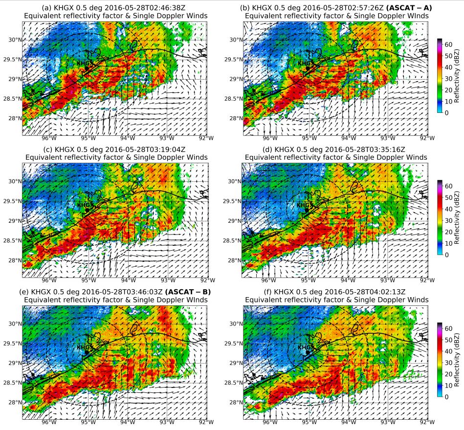
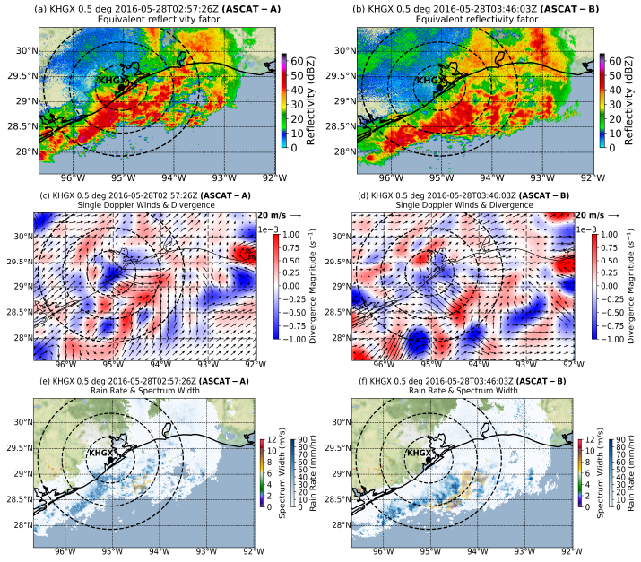
3.3. Ground Radar Processing

The radar analysis was performed using the Python Atmospheric Radiation Measurement (ARM) Radar toolkit (Py-ART; [46]), which is an open-source Python module containing a collection of weather radar algorithms and utilities for data processing and visualization. The first step was to perform a quality control of the data that included de-aliasing of the radial velocity field, removal of non-meteorological targets (e.g., insects) via thresholds on various polarimetric variables [47], and correction for attenuation, clutter, and second-trip contamination. Cartesian gridding of the data was performed at 225 × 225 horizontal domain (corresponding to 3.5 km grid spacing) and 40 vertical levels (corresponding to 500 m). The rainfall estimation is based on the algorithm developed by Cifelli et al. [48], referred to as CSU-HIDRO, which is coded in a Python package named CSU_RadarTools [49].
A single-Doppler analysis algorithm was applied to the radar data prior to the Cartesian gridding, utilizing 2DVAR approach of Xu et al. [50], which is an extension of the Velocity Azimuth Display (VAD) technique [51]. More specifically, after basic quality control, a background wind field is created using the traditional VAD analysis of radar data. Then, the raw radial velocity data is used to apply an optimal correction to the background winds, based on their error covariances. This method retrieves high-quality low-level 2-D Doppler vector winds on the conical radar scan surface, which are comparable to scatterometers’ performance (∼0 bias, ∼2 m s 1 speed and ∼20 direction errors, 0–32 m s 1 valid range; [52]), but have much finer resolution in space and time with no degradation in the presence of precipitation. The output velocity vector field obtained by our single-Doppler analysis has a spatial resolution of 3 km. For the purpose of this study, Doppler winds at only the lowest elevation sweep (0.5 ) were used to identify near-surface wind features.

3.4. Scatterometer Wind Retrieval Correction

Single-Doppler analysis winds provide an estimate of the local wind field that is unaffected by attenuation in the presence of rain, in contrast to scatterometer wind retrievals that can be affected by rain rates as low as 6 mm h 1 [53]. Moreover, the inability of weather forecasting models to resolve mesoscale phenomena can further complicate the ambiguity selection process, leading to false ambiguity wind selection. The winds retrieved by Doppler radars are reported at an increasing height with distance due to the earth’s curvature. At relatively close distances from the radar they can be representative of the near-surface wind conditions [33] and therefore be used to correct the low-quality scatterometer retrievals over precipitation. This process entails the manual examination of the scatterometer’s multiple/unambiguous wind direction solutions within a wind vector cell, which in the presence of rain should be more than 2 with similar probabilities, and the selection of the one that more closely matches the Doppler wind direction. Elevated magnitude of wind shear at the low levels of the troposphere is more conducive to generation of quasi-linear convective system [54], which can complicate the proposed correction of the wind direction. Using information of the MCS’s location and precipitation one can approximate the wind direction by relying on (radial) outflow processes.

3.5. Resampling of Background Winds

The ambiguity selection process was applied on the UHR product for 3 NWP models; i.e., ECMWF, MERRA-2 and RAP. The ECMWF and MERRA-2 models provided winds at a global scale, whereas the RAP winds were confined over the North America and adjacent oceanic regions. The ECMWF winds where obtained directly from the ASCAT L2 product and had 12.5-km spatial resolution. The MERRA-2 model global winds (tavg1_2d_ocn_Nx product) were available at 7-km spatial resolution through the UHR process. RAP winds were available at a native 13-km resolution horizontal grid and 3-h temporal resolution, and therefore were resampled at a 7-km prior to ingest them in the ambiguity removal process using the pyresample module [55]. This Python module is a fast and generalized interface to resample (reproject) Earth-observing satellite data, both gridded and swath types, by the implementation of a (custom) KD-tree approach.

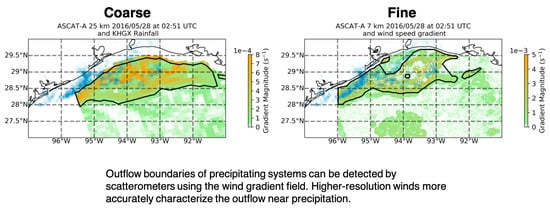
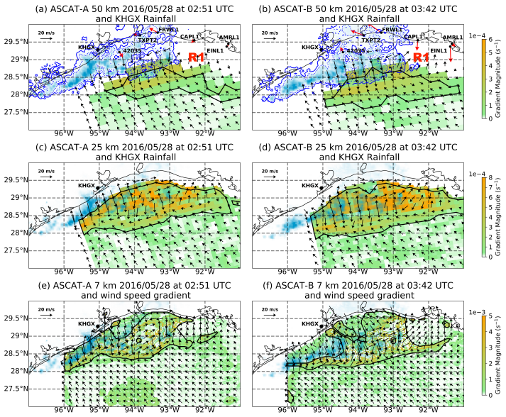
4. Results and Discussion

4.1. Outflow Boundary Detection

The method described in the previous sections has been applied to a severe weather system, located along the coastal U.S., in order to demonstrate the utility of the UHR product to identify small scale features along an outflow boundary and how those are related to features captured by the lower resolution ASCAT products. First, the method is applied on the lower resolution products, 25-km and 12.5-km, to provide a more abstract form of the detected outflow boundaries. The wind vectors are analyzed along the boundaries and at the vicinity of precipitation associated with them. Subsequently, the method is applied on the UHR product. The results are evaluated based on the precipitation retrievals from ground-based radars and characteristics of the UHR retrieval. In this context, the outflow boundary features detected by the coarser resolutions are considered as truth in order to evaluate the UHR detections, at least at the vicinity of the precipitating system.
An MCS was present over Houston (TX) on 28 May 2016 that coincided with the overpasses of the MetOp satellite series and was within the range of the KHGX radar. Ground-based radars are a valuable platform to study and detect features associated with convective systems [33,56,57,58]. The evolution of the MCS is depicted in Figure 1 by the radar reflectivity and single-Doppler radar wind-field retrieved at the lowest elevation angle. The overpasses of ASCAT-A and ASCAT-B at the closest times relative to the radar are also indicated (Figure 1b,e). The reflectivity field indicated that the system was slowly moving toward the southeast with the highest reflectivity magnitude reaching 56 dBZ within the convective core. An extensive stratiform region was visible at 3:35 UTC onwards (Figure 1d–f). During the last time step (Figure 1e,f) the system started to dissipate as the reflectivity magnitude decreased within the stratiform and regions of the main convection, although regionally the highest reflectivity remained the same. This reflectivity structure within the MCS is in line with the detailed analysis of MCS in Houze [59]. A similar case of a squall line was studied in Smull and Houze [60]; however, their case was strictly over land. The authors used reflectivity radar data to show that the system propagated towards the east-southeast and system-relative Doppler horizontal velocity to identify the presence of a rear-inflow jet (RIJ), and a gust front marked by strong low-level convergence. Doppler winds at the lowest scanning elevation angle can be representative of the near surface wind-conditions depending on the distance from the radar. Figure 1 was created to identify the structure and propagation of the MCS, along with the kinematic characteristics of the flow. The range rings during the overpasses (Figure 1b,e) are spaced at 50-km distance, where the retrievals at 100 km and 150 km from the radar location are obtained at a height of 1.5 km and 2.8 km, assuming standard beam-propagation conditions. The analysis revealed the presence of a descending rear-to-front flow that was characterized by a strong northwesterly flow reaching a height of 1.5-km. The descending flow (RIJ) typically forms as a response of the latent heat released by sublimation, melting and evaporation below the trailing-stratiform cloud Houze [59]. The RIJ was present during all time steps, fueling the MCS. The increase in the wind speed over a rear-inflow jet was also observed by Keene and Schumacher [61], who used observations and simulations to understand the mechanisms responsible for the initiation and maintenance of a convective line.

4.2. Impact of Different Scatterometer Product Resolutions

Klingle et al. [56] analyzed 9 cases in order to identify characteristics of gust fronts observed by a Doppler radar located in Norman, OK. The average maximum and minimum height of the respective gust fronts was 2.6 and 0.8 km, respectively. The authors found that the gust fronts can be detected as thin lines of echoes in the reflectivity field with a maximum of 7 dBZ. However, this feature becomes apparent at a later stage of the storm’s lifecycle, after the gust front has moved away from the parent storm. Similar cold pool characteristics were identified by Borque et al. [62], while also noting insect-related dual polarization radar signatures in the gust front. Additionally, turbulence that is present between the outflow boundary and the environmental flow can be identified as lines of enhanced spectrum width (e.g., [63]), thus indicating the presence of the gust front. Figure 2 was created to test the detection of the outflow boundary in any of the aforementioned radar fields. At the overpass of ASCAT-A there was no apparent line of low reflectivity echoes (Figure 2a) in front of the MCS, which could be attributed to the height of the outflow boundary relative to the distance from the radar. The outflow boundary should have been present at least about 100 km away from the radar (Figure 2a, middle concentric), which corresponds to reflectivity retrievals at a height of at least 1.5 km. It is probable that the beam was above the outflow, thus minimizing the detection of the outflow boundary in this case.
The Doppler-retrieved winds (Figure 2c) were northwesterly within the precipitating system and shifted south-southwesterly in front of the MCS, where convergence was observed along its boundary. Although, the outflow boundary was not prevalent in the reflectivity field, single-Doppler analysis winds captured a shift to south-southwesterly flow along the boundary of the MCS, which might indicate the presence of a deep outflow boundary embedded at the edge of the system.
Similar to ASCAT-A, at the overpass of ASCAT-B there was no apparent line of low reflectivity echoes (Figure 2b) in front of the MCS.
The Doppler wind field (Figure 2d) captured backing winds over the precipitating system, close to the time of ASCAT-B overpass. A large area of divergence was present in front of the system, at 100 km distance from the radar (middle dashed circle). Over the same area and in front of the heavy precipitation, elevated values of spectrum width were observed, with highest value of 11 m s 1 (Figure 2f). However, the linearity of the feature observed by Klingle et al. [56] at low levels was not present in this case. An indication of the presence of the outflow boundary could be deduced from the above observations, while at the same time the rear-to-front flow was also detected in the wind analysis field.
Scatterometer wind retrievals encompass a set of solutions (up to 4) for each wind vector cell, with the first two being of opposite direction due to the sinusoidal nature of the GMF. Figure 3 depicts the wind retrievals for ASCAT products of 50-km spatial resolution after the directional ambiguity removal (Figure 3a,b), along with the available wind solutions (Figure 3c–f) obtained through the GMF. Wind solutions 3 and 4 exhibited increased wind variability and are not presented here, as these solutions suffered from a known effect of rain, i.e., the alignment of the wind vectors perpendicular to the satellite track [64,65]. Wind retrievals at 50-km resolution are absent close to the coast due to potential land contamination. The wind field for both ASCAT-A and -B was southeasterly over the precipitation system (Figure 3a,b). The ECMWF model winds, used during the ambiguity removal process, also indicated southeasterly flow over the whole domain (Figure 7a,b), failing to resolve the mesoscale system. Over the same area single-Doppler analysis wind field indicated northwesterly flow (Figure 3a; red streamlines).
The correction method described in the methodology section was applied to rain-afflicted ASCAT wind vectors, offshore of Houston, where the ambiguity removal process most likely failed. Around 28.7 deg N and 94.5 deg W wind retrievals were flagged by the MLE for both ASCAT-A and -B (Figure 3c–f; gold vectors), indicating large distance between the ambiguous solution 1, 2 from the GMF and ECMWF background winds. Large values for the MLE might indicate that the retrieval is contaminated by rain or confused sea state. Not surprisingly, this area was severely affected by high rain rates (Figure 2e; 70 mm h 1 ), therefore the Doppler retrievals should have been more representative of the wind field than the scatterometer winds. In the absence of any other observations, the observed sounding at KLCH station at 12 UTC indicated a uniform wind flow (southwesterly) up to height of 1.5 km, therefore the correction method was applied to scatterometer wind vectors up to 100 km radial distance from the radar location. For example, the first wind solution for ASCAT-A (Figure 3c) captured north-northwest wind direction over the respective region, whereas the second wind solution (Figure 3e) indicated south-southeast wind direction, with the latter being the solution selected by the ambiguity process. The single-Doppler analysis wind field (Figure 2c) captured north-northwest wind direction over an area that expanded radially outwards from the location of the radar. For each wind vector cell that fell within the radar domain, the wind direction of the optimal solution was substituted with the Doppler-compliant unambiguous wind direction; i.e., north-northwest (Figure 3c, wind solution 1). The suggested wind solution was was then constructed for all ASCAT wind retrievals at 50-km.
The aforementioned approach was applied to the 25-km spatial resolution product (Figure 4). Wind retrievals were available closer to the coast, but the wind vectors exhibited significant variability in comparison to the coarser resolution, owing to the presence of the precipitating system. Once again, the ambiguity selection process likely erroneously indicated southerly flow over the radar-derived streamlines for both ASCAT-A (Figure 4a) and -B (Figure 4b).
ASCAT wind products at 7-km spatial resolution (Figure 5a,b) had the same response as the coarser wind products. Although the shift in the wind direction was an indication of the mesoscale system, the wind direction was wrong. Independent of the absence of a proper rain flag, the model winds played an important role in the selection of the wind direction. An evaluation of the available solutions (Figure 5c–f) was performed to obtain the wind direction that was in accordance with the low-level feature identified in the radar analysis. In turn the suggested wind field altered the structure of scatterometer wind field and its products near the precipitation region, such as the wind gradient, convergence and vorticity.
In front of the MCS all three ASCAT products showed a response by the winds to the cold-pool outflow (Figure 6). The valid wind retrievals at all 3 spatial resolutions indicated southeasterly flow over the open ocean. At the overpass of MetOp-A satellite, winds at 50-km resolution captured a sudden shift in the wind direction from southeasterly to northerly flow along the border of the precipitating system (Figure 6a, blue-dotted line), and an increase in the wind speed from 10 to 18 m s 1 . The system was characterized by high rainfall rates, reaching a local maximum of 130 mm h 1 . Over the precipitation region the wind vectors were characterized by increased speed and northerly flow, though the increase in the wind speed could be attributed to the effect of rain on scatterometers [27,65,66,67]. The presence of the rear-inflow jet ensured a wind maximum that started at or below 500 m above ground level, as friction near the surface prevented a rise in the wind speed to reach this maximum (logarithmic wind profile). At the eastern side of the domain and away from the precipitation (Figure 6a; R1), wind retrievals indicated southwesterly flow. Further south of the respective region (below 28.8 N) the wind direction shifted abruptly to northwest. However, the ECMWF model winds used in the ambiguity selection process indicated southeasterly flow over the whole domain (Figure 7). The coastal buoy observations of wind speed and direction for all stations were also examined before and after ASCAT overpasses to ensure that the buoys were operating normally. The observations indicated abnormal behavior of the buoys during this time and were suspicious, therefore, the ambiguity removal solutions were considered here as likely correct wind vectors. Scatterometers retrieve winds near the surface; i.e., equivalent neutral winds, therefore the wind gradient should have a distinctive signature, especially at the boundaries of the horizontally expanding cold air. The changes in the wind field induced by the outflow boundary were depicted in the wind gradient field, where the magnitude increased from near zero value in the open ocean to 3 × 10 4 s 1 within the system (Figure 6a). The two thresholds used in the GF algorithm for the 50-km retrievals were 6.8 × 10 5 s 1 and 1.2 × 10 4 s 1 , respectively. A unique GF (Figure 6a, black polygon) was identified that extended about 200 km in horizontal distance and located in front of the system.
At the overpass of MetOp-B satellite, the system had propagated further away to the open ocean, towards the southeast, and it was characterized by intense precipitation with maximum rain rate of 100 mm h 1 (Figure 6b). Over convective core of the system high values of wind gradient existed, reaching a maximum of 6 × 10 4 s 1 , associated with wind variability over intense rain rates. At the eastern side of the system (Figure 6b, R1) the wind had a similar response to ASCAT-A. In front of the system the wind gradient was characterized by higher values than at the overpass of ASCAT-A, indicating a more vigorous outflow boundary, which might have emanated from intersecting boundaries of nearby convective cores. The gradient wind feature (Figure 6b, black polygon) expanded outwards but in a more confined shape than ASCAT-A, probably denoting the presence of a well-defined outflow boundary. The thresholds used in the GF process were the same as for ASCAT-A since both ASCAT instruments are well calibrated with each other and have similar performance [68,69].
A sensitivity test was performed on the two thresholds to capture differences in the population of the gradient wind features, owing to smaller-scale wind features that could be associated with the MCS and its evolution. The primary threshold removes the background noise and the secondary accounts for the bias due to lower wind gradients. The primary (secondary) threshold used in the GF method varied from 1 − 9 × 10 5 ( 10 4 ). The results indicated that there was no change in the number of features, thus providing additional confirmation that wind vectors at 50-km spatial resolution cannot resolve smaller than mesoscale wind features.
The coastal wind product at 25-km spatial resolution provides retrievals as close as 50 km from the coast (Figure 6c,d). At the overpass of ASCAT-A (Figure 6c) many of the coastal wind vectors were contaminated by rain, therefore the suggested wind field provided a more realistic solution. Once again, wind speed within the precipitation system reached a maximum of 24 m s 1 , whereas over the open ocean the maximum was 10 m s 1 . In front of the MCS’s precipitation boundary (Figure 6c, blue line), wind vectors associated with the expanding outflow boundary shifted from southeast to east. Wind gradient magnitude increased over the same area to a maximum of 0.5 × 10 3 s 1 . Within the system, elevated values of wind gradient were locally confined near intense precipitation. A unique GF was identified that encompassed part of the precipitating system as well as the associated outflow boundary (Figure 6c, black solid line).
The primary and secondary thresholds used in the GF algorithm were 6.8 × 10 5 s 1 and 1.2 × 10 4 s 1 , respectively. Garg et al. [23] evaluated the GF method using thresholds determined by a model simulation. Based on statistical indices—i.e., critical success index, false alarm and bias ratio—the authors obtained a value of 6.8 × 10 5 s 1 and 1.2 × 10 4 s 1 for the primary and secondary thresholds, respectively. The same sensitivity test performed on the ASCAT-A wind gradient process had similar results to the coarser wind product. Kilpatrick and Xie [26] hypothesized that ASCAT wind retrievals at 25-km spatial resolution failed to detect convective-scale gust fronts because the product’s resolution is too coarse to resolve such phenomena.
At the overpass of ASCAT-B (Figure 6d) the wind direction shifted to easterly in front of the border of the precipitation (Figure 6d, blue line). Wind direction within the system was northerly, according to the suggested solution. The wind gradient increased from near zero at the open ocean to 0.62 × 10 3 s 1 towards the boundary of the precipitation. On the eastern side of the MCS (Figure 6d, R1), elevated values of wind gradient were associated with variable wind direction and speed on the contrary with the uniform wind field depicted by ASCAT-A. Single-Doppler analysis winds (Figure 1e) over the same area indicated a shift in the wind for distances longer than 150 km from the radar location; although at such distances the wind vectors didn’t correspond to a low-level field, they might be representative of a deep gust front layer. The unique GF (Figure 6d, black solid line) extended further east near the coastline and included the shift in the wind vectors induced by the outflow boundary, thus supporting the utility of this method for the detection of such phenomena. The primary and secondary threshold values used in the GF algorithm were 2.2 × 10 4 s 1 and 1.8 × 10 4 s 1 , respectively. The sensitivity test on the thresholds used in the GF algorithm affected only the size of the feature and not the population.
UHR adjusted wind retrievals at the overpass of ASCAT-A (Figure 6e) were available as close as 10 km from the coast. Offshore Houston winds were characterized by northwesterly flow with high wind speeds reaching a maximum of 30 m s 1 . A buoy located at 29.3 N 94.4 W (Figure 6a, 42035) indicated northerly direction (350 N) at the closest time to the ASCAT-A overpass, in accordance with the UHR retrievals near the coast. However, some wind retrievals were suspect due to land contamination and/or precipitation. Rain-afflicted wind vector were aligned perpendicular to the MetOp-A track (ascending, towards northwest) near the center of the domain. In the eastern side of the domain (Figure 6a, R1) the wind was southerly (Figure 6e), over an area not affected by precipitation. However, at about 29 N 92 W, a wind shift to southwesterly winds was observed, which was characterized by elevated wind gradient values (2.7 × 10 3 s 1 ). In front of the precipitating system winds shifted to southwesterly in contrast to the direction indicated by the coarser resolutions. The wind gradient magnitude over the area was reached a local maximum of 4 × 10 3 s 1 .
Differences in the wind vectors between the UHR and the coarser resolution might have arisen from differences in the retrieval algorithms, as well as from the different model winds used in the ambiguity selection. While ASCAT winds at 50- and 25-km spatial resolution implement the ECMWF model for the MLE estimator, UHR process uses model winds from MERRA-2. Portabella and Stoffelen [18] found that 50-km ASCAT winds performed better than ECMWF model winds against buoy wind measurements in the presence of rain-induced downdraft, pointing out that ECMWF does not resolve well the airflow near rain.
Two main GFs were obtained in this case, for the primary and secondary threshold values of 6.8 × 10 4 s 1 and 2 × 10 3 s 1 , respectively. Other smaller features behind the MCS were spurious due to the aforementioned low-quality retrievals. UHR spatial resolution allowed for small variations in the wind that could lead to a larger bias in the wind gradient field in comparison with the coarser resolution, therefore the secondary threshold used in the GF method was an order of magnitude higher. The GF that was characterized by the largest area, encompassed a large part of the precipitation. However, in front of the MCS, the outline of the feature was in agreement with the precipitation structure near the surface and the precipitation-induced outflow boundary. The feature offshore the coast of Houston was associated with increased wind gradient magnitude over an area that was affected by precipitation (Figure 6e). The radar analysis over the respective area (Figure 1), didn’t reveal any change in the wind field before and after the overpass, which might have indicated that scatterometer wind retrievals were of low quality.
At the overpass of ASCAT-B (Figure 6f) elevated wind speed magnitude (30 m s 1 ) was retrieved within the precipitating system, while the suggested wind direction was northwesterly. Wind gradient magnitude was small due to the homogeneity of the vectors over the area. A buoy located at 29.3 N 94.4 W (Figure 6b, 42035) indicated southeasterly direction (153 N) at the closest time to the ASCAT-A overpass; however, measurements taken 30 min earlier (obtained every 10 min) reported northwesterly to northeasterly direction. Considering the delay in the response of the scatterometer at sudden wind changes, the surrounding UHR retrievals near the coast were in accordance with previous buoy measurements (Figure 6f). On the eastern side of the domain (Figure 6b, R1), the wind was southwesterly over an area free of precipitation (Figure 6f). In front of the system’s precipitation border the wind direction shifted to southwesterly, with speed of the same magnitude (19 m s 1 ) as over the open ocean. The wind gradient field was characterized by fragments and large variations in magnitude along the front edge of the MCS. Fragments within the gust front have also being observed by high-resolution Doppler radars Uyeda and Zrnic [70], providing confidence that the 7-km resolution product can detect such fine-scale features.
Multiple wind gradient features were identified in the UHR product during the overpass of ASCAT-B (Figure 6f, black solid polygons), with the largest feature capturing the wind shift in front of the MCS associated with the outflow boundary. The wind feature at the most eastern part of the domain (29.4 N 91.7 W) was characterized by wind gradient maximum, induced by a sudden change in the wind direction from southerly to northerly over the respective area. Two buoys (Figure 6b, AMRL1 and EINL1) located near the coast, measured northwesterly and northerly wind direction, respectively, indicating that the UHR retrieval was valid. Further north, two small features near the coast (29.5 N 92.2 W) were also related to a wind shift; however, in this case the buoy (Figure 6b, CAPL1) located near them measured northeasterly wind direction. To note, the standard meteorological data product reported wind speed and direction at 6 min interval time, however many invalid measurements were present in both variables, probably due to malfunction during this time period. Offhsore Houston, another GF was present that included spurious retrievals under the effect of rain.

4.3. Effects of Background Winds on Scatterometer Retrievals

A critical component of the ambiguity removal process is the input of background winds, which are typically provided by a weather model. It has been shown that national weather prediction (NWP) model biases are due to mesoscale processes, e.g., convection, which are resolved by the scatterometers but not by models [71]. Portabella et al. [53] investigated the rain effects on ASCAT-retrieved winds and found that the ECMWF winds did not resolve well high-wind-variability cases, such as downdraft-like wind patterns, due to the coarse spatial resolution. In the same study, the inability of the ECMWF to resolve wind variability under rainy conditions was also observed.
A distinctive signature of a well-organized MCS is the cold pool [1] that develops near the surface as radially expanding winds, producing gusty winds [72].
At the overpass of ASCAT-A ECMWF (Figure 7a) indicated southeasterly flow with constant wind speed over the domain. A similar response to the winds was also captured by MERRA-2 (Figure 7b). Buoys near the coast measured winds coming from variable directions, indicating that there was at least some wind variability present. More specifically, buoy 42035, located within the precipitation area, measured northwesterly direction. Considering the inability of the ECMWF to wind variability under rainy conditions Portabella et al. [53] and the buoy measurements, it is evident that both models failed to capture surface wind features associated with the presence of the MCS. On the contrary, the RAP model (Figure 7c) clearly captured wind speed and direction changes in front and within the system itself. In front of the MCS, over the western side, wind speed magnitude was decreased substantially, which could be attributed to opposing winds over the convergence zone. Variable wind direction was observed by the model at the eastern side of the domain, near the buoys EINL1 and AMRL1. Surprisingly, the low wind speed magnitude observed by the buoys was also captured by the models. Around an area centered at 28.7 N 95.5 W the wind direction shifted to northwesterly with increased speed capturing the RIJ that was also observed by the radar analysis wind field (Figure 1b). Around 29 N 91.6 W, the RAP winds were variable in direction and speed magnitude. Importantly, the UHR-wind gradient magnitude was elevated over the same area (Figure 6e), which was also included in the gradient feature, providing evidence that the UHR is able to identify wind features not related to convective systems.
At the overpass of ASCAT-B, wind direction retrieved by ECMWF (Figure 7d) and MERRA-2 (Figure 7e) remained southeasterly throughout the domain at the same wind speed. At the western side of the system, the decreased wind speed area had expanded along the precipitation boundary, as well as towards the open ocean probably denoting a vigorous outflow boundary. Behind the system wind direction was southeasterly in contrast with the radar-derived wind analysis field (Figure 1e). Buoy station CAPL1 measured northerly wind with high speed magnitude, whereas RAP captured easterly direction with moderate speed, which was higher than at the overpass of ASCAT-A (Figure 1c). Near buoy station AMRL1, wind speed magnitude and direction was variable, which was also indicated by a nearby station (EINL1) that measured northerly direction and high speed magnitude. Not surprisingly, UHR-wind gradient magnitude was elevated and enclosed in a gradient feature over the same area (Figure 6f).
In order to examine the response of the UHR retrievals to the background wind field, Figure 8 was created, which depicts the divergence field calculated from the UHR wind retrievals as a result of the ambiguity removal process from the MERRA-2 and RAP models. ECMWF and MERRA-2 wind field had nearly-identical wind direction (southeasterly) over the domain, therefore only MERRA-2 winds were used in the ambiguity removal process. The wind divergence field obtained from UHR-MERRA-2 winds at the overpass of ASCAT-A (Figure 8a) captured divergence along the front edge of the MCS. On the contrary, UHR-RAP (Figure 8b) captured convergence over the same area. Fuglestvedt and Haerter [73] found that as cold pools spread out along the surface, they form a surge of flow that leads to moisture convergence induced by the low-level wind. At the overpass of ASCAT-B the UHR-MERRA-2 (Figure 8c) and UHR-RAP (Figure 8d) divergence field has the same response as in the overpass of ASCAT-A, i.e., divergence and convergence, respectively. Thus, the depiction of low-level wind features associated with convective systems depend to a large degree on the accurate representation of the background winds. This analysis also supports the usage of the wind gradient as more independent metric to capture outflow boundaries, as natural characteristics can complicate the interpretation of the divergence field.

5. Summary and Conclusions

In this study we applied a novel technique based on the wind gradient, termed gradient feature method Garg et al. [23] to identify outflow boundaries induced by MCSs from scatterometer data. Such systems produce intense precipitation at the ocean’s surface, which can degrade the quality of scatterometer retrievals. To mitigate these effects we adjust the retrievals of rain-afflicted wind vector cells by examining the available solution obtained from the GMF and ground-based radar single-Doppler analysis wind retrievals. In order to assess the ability of scatterometers to accurately captured low-level wind features associated with convective systems, we examine the response of ASCAT wind retrievals on the different background winds as a result of the ambiguity removal process.
Leveraging the close time interval of overpasses between the MetOp-A and -B satellites, the GF method was applied over an MCS located offshore of Houston for adjusted wind retrievals at spatial resolutions of 50-, 25- and 7-km. An increase in the wind speed was observed in front of the MCS by all resolutions, whereas the change in the wind direction was more variable. Increased wind gradient magnitude was also observed by all resolutions, indicating the ability of the method to detect outflow boundaries. Noticeably, the wind gradient magnitude for the 50-km product ( 10 4 s 1 ) was one order of magnitude less than the 25- and 7-km ( 10 3 s 1 ), since smoothing at the coarser resolution can obscure sudden changes in the wind speed and/or direction, thus leading to much smoother variation between adjacent wind vector cells. Differences in the wind gradient field were also observed between the 25-km and 7-km product, with the latter capturing fragments and larger variations in magnitude along the front edge of the MCS.
At all three resolutions, a gradient feature was captured that encompassed a large area of the MCS and its outflow boundary. The area of the GF increased with resolution as more wind vectors were available close to the coast. The importance of spatial resolution became apparent by looking at the location of the GF-detected outflow boundary relative to the MCS. In the 25-km product, the gradient feature included an area that extended further outwards from the 1 mm h 1 rainfall rate border, whereas in the 7-km, the feature was within the edge of the precipitation. This indicated that the high resolution product identified a more detailed structure of the outflow boundary that can be associated with its evolution. Additionally, smaller-scale features at 7-km resolution were also detected by the GF method, however, their nature was uncertain due to a lack of buoy observations over the respective area.
Scatterometer wind retrievals depend on the background wind field obtained from weather models, which is an input in the ambiguity selection process. Global models are characterized by low spatial resolution and therefore are unlikely to detect mesoscale phenomena. In this study, 25-km ECMWF and MERRA-2 winds failed to accurately simulate winds near the MCS, instead showed uniform wind speed and direction over the domain. The 13-km RAP model was able to detect surface-wind modulations induced by the MCS throughout the overpasses of ASCAT-A and -B. Buoy wind measurements along the coast of the domain were also in better agreement with the RAP winds, providing confidence that the simulated wind field was more correct. The difference between the retrieval products became important in the divergence field, where divergence in front of the MCS using UHR-MERRA-2 wind field was replaced by convergence by the UHR-RAP. Additionally, this analysis supports the use of the wind gradient field as a more independent metric to capture surface wind features than the divergence [23].
Additional case studies need to be investigated to draw more robust conclusions on the detection of outflow boundaries using the GF method, especially in the case of smaller convective systems, where the utility of the 7-km product is of primary importance. Ku-band scatterometers have been providing valuable wind measurements over the ocean, however the retrieval process is affected by the sea surface temperature (SST) [74] and to a larger degree by rain [64], due to the wavelength dependence on scattering ( λ 4 ) in comparison to the C-band. Several studies have explored solutions to mitigate these effects [75,76] and validated the performance of Ku-band against C-band scatterometers [77,78]. Considering the characteristics of MCSs, Ku-band scatterometers might provide a more accurate depiction of the outflow and precipitation boundary. The extend to which the GF method can be applied to scatterometers operating at higher frequencies needs to explored, especially the physical significance of its thresholds.

Author Contributions

Conceptualization, T.J.L.; methodology, T.J.L., G.P., P.G., S.W.N., R.D.L.; software, G.P.; validation, G.P., T.J.L.; formal analysis, G.P.; investigation, G.P., T.J.L.; resources, T.J.L., T.C.; data curation, G.P.; writing–original draft preparation, G.P.; writing–review and editing, G.P., T.J.L., P.G., S.W.N., R.D.L.; visualization, G.P.; supervision, T.J.L., T.C.; project administration, T.J.L., T.C.; funding acquisition, T.J.L., T.C. All authors have read and agreed to the published version of the manuscript.

Funding

This research was funded by NASA’s Ocean Vector Winds Science Team (OVWST) grant number NNH13ZDA001N-OVWST.

Acknowledgments

The authors would like to credit the Py-Art and Pytroll community. The ASCAT data were gathered from EUMETSAT through the Earth Observation Portal. NEXRAD data were gathered from the NOAA’s NCEI and buoy data from the NOAA’s NDBC. Winds components were collected from NASA’s Earthdata web application that is built on top of NASA’s Common Metadata Repository, as part of the Earth Observing System Data and Information System project.

Conflicts of Interest

The authors declare no conflict of interest. The funders had no role in the design of the study; in the collection, analyses, or interpretation of data; in the writing of the manuscript, or in the decision to publish the results.

Abbreviations

The following abbreviations are used in this manuscript:
ARMAtmospheric Radiation Measurement
ASCATAdvanced Scatterometer
AWDPASCAT Wind Data Processor
C-MANCoastal-Marine Automated Network
CSUColorado State University
DYNAMODYNAmics of Madden-Julian Oscillation
ECMWFEuropean Centre for Medium-Range Weather Forecasts
EUMETSATEuropean Organization for the Exploitation of Meteorological Satellites
GFGradient Feature
GMFGeophysical Model Function
L1BLevel 1b
L2Level 2
MERRA-2Modern-Era Retrospective Analysis for Research and Applications
MetOpMeteorological Operational
MCSMesoscale Convective System
MLEMaximum Likelihood Estimation
NASANational Aeronautics and Space Administration
NCEINational Centers for Environmental Information
NDBCNational Data Buoy Center
NOAANational Oceanic and Atmospheric Administration
NWPNational Weather Prediction
Py-ARTPython ARM Radar Toolkit
RAPRapid Refresh
RIJRear-Inflow Jet
SRFSpatial Response Function
SSTSea Surface Temperature
TRMMTropical Rainfall Measurement Mission
UHRUltra-High Resolution
UTCUniversal Time Coordinated
VADVelocity Azimuth Display
VarQCVariational quality control flag
WRFWeather Research and Forecasting
2DVAR2-D variational

References

  1. Corfidi, S.F. Cold pools and MCS propagation: Forecasting the motion of downwind-developing MCSs. Weather Forecast. 2003, 18, 997–1017. [Google Scholar] [CrossRef]
  2. Nesbitt, S.W.; Cifelli, R.; Rutledge, S.A. Storm Morphology and Rainfall Characteristics of TRMM Precipitation Features. Mon. Weather Rev. 2006, 134, 2702–2721. [Google Scholar] [CrossRef] [Green Version]
  3. Yuan, J.; Houze, R.A., Jr. Global variability of mesoscale convective system anvil structure from A-Train satellite data. J. Clim. 2010, 23, 5864–5888. [Google Scholar] [CrossRef]
  4. Houze, R.A. 100 years of research on mesoscale convective systems. Meteorol. Monogr. 2018, 59, 17.1–17.54. [Google Scholar] [CrossRef]
  5. Young, G.S.; Perugini, S.M.; Fairall, C. Convective wakes in the equatorial western Pacific during TOGA. Mon. Weather Rev. 1995, 123, 110–123. [Google Scholar] [CrossRef] [Green Version]
  6. Weaver, J.F.; Nelson, S.P. Multiscale aspects of thunderstorm gust fronts and their effects on subsequent storm development. Mon. Weather Rev. 1982, 110, 707–718. [Google Scholar] [CrossRef] [Green Version]
  7. Forbes, G.S.; Wakimoto, R.M. A concentrated outbreak of tornadoes, downbursts and microbursts, and implications regarding vortex classification. Mon. Weather Rev. 1983, 111, 220–236. [Google Scholar] [CrossRef] [Green Version]
  8. Wilson, J.W.; Schreiber, W.E. Initiation of convective storms at radar-observed boundary-layer convergence lines. Mon. Weather Rev. 1986, 114, 2516–2536. [Google Scholar] [CrossRef] [Green Version]
  9. Wilson, J.W.; Foote, G.B.; Crook, N.A.; Fankhauser, J.C.; Wade, C.G.; Tuttle, J.D.; Mueller, C.K.; Krueger, S.K. The role of boundary-layer convergence zones and horizontal rolls in the initiation of thunderstorms: A case study. Mon. Weather Rev. 1992, 120, 1785–1815. [Google Scholar] [CrossRef] [Green Version]
  10. Feng, Z.; Hagos, S.; Rowe, A.K.; Burleyson, C.D.; Martini, M.N.; de Szoeke, S.P. Mechanisms of convective cloud organization by cold pools over tropical warm ocean during the AMIE/DYNAMO field campaign. J. Adv. Model. Earth Syst. 2015, 7, 357–381. [Google Scholar] [CrossRef] [Green Version]
  11. Moncrieff, M.W.; Liu, C.; Bogenschutz, P. Simulation, modeling, and dynamically based parameterization of organized tropical convection for global climate models. J. Atmos. Sci. 2017, 74, 1363–1380. [Google Scholar] [CrossRef]
  12. Thorpe, A.; Miller, M.; Moncrieff, M. Two-dimensional convection in non-constant shear: A model of mid-latitude squall lines. Q. J. R. Meteorol. Soc. 1982, 108, 739–762. [Google Scholar] [CrossRef]
  13. Wang, Z.; Stoffelen, A.; Fois, F.; Verhoef, A.; Zhao, C.; Lin, M.; Chen, G. SST dependence of Ku-and C-band backscatter measurements. IEEE J. Sel. Top. Appl. Earth Obs. Remote Sens. 2017, 10, 2135–2146. [Google Scholar] [CrossRef]
  14. Long, D.G.; Collyer, R.; Arnold, D.V. Dependence of the normalized radar cross section of water waves on Bragg wavelength-wind speed sensitivity. IEEE Trans. Geosci. Remote Sens. 1996, 34, 656–666. [Google Scholar] [CrossRef] [Green Version]
  15. Kumar, R.; Bhowmick, S.A.; Chakraborty, A.; Sharma, A.; Sharma, S.; Seemanth, M.; Gupta, M.; Chakraborty, P.; Modi, J.; Misra, T. Post-launch calibration–validation and data quality evaluation of SCATSAT-1. Curr. Sci. 2019, 117, 973. [Google Scholar] [CrossRef]
  16. Bhowmick, S.A.; Cotton, J.; Fore, A.; Kumar, R.; Payan, C.; Rodríguez, E.; Sharma, A.; Stiles, B.; Stoffelen, A.; Verhoef, A. An assessment of the performance of ISRO’s SCATSAT-1 Scatterometer. Curr. Sci. 2019, 117, 959. [Google Scholar] [CrossRef]
  17. Misra, T.; Chakraborty, P.; Lad, C.; Gupta, P.; Rao, J.; Upadhyay, G.; Kumar, S.V.; Kumar, B.S.; Gangele, S.; Sinha, S.; et al. SCATSAT-1 Scatterometer: An improved successor of OSCAT. Curr. Sci. 2019, 117, 941. [Google Scholar] [CrossRef]
  18. Portabella, M.; Stoffelen, A. Rain detection and quality control of SeaWinds. J. Atmos. Ocean. Technol. 2001, 18, 1171–1183. [Google Scholar] [CrossRef]
  19. Vogelzang, J.; Stoffelen, A.; Verhoef, A.; De Vries, J.; Bonekamp, H. Validation of two-dimensional variational ambiguity removal on SeaWinds scatterometer data. J. Atmos. Ocean. Technol. 2009, 26, 1229–1245. [Google Scholar] [CrossRef]
  20. Figa-Saldaña, J.; Wilson, J.J.; Attema, E.; Gelsthorpe, R.; Drinkwater, M.R.; Stoffelen, A. The advanced scatterometer (ASCAT) on the meteorological operational (MetOp) platform: A follow on for European wind scatterometers. Can. J. Remote Sens. 2002, 28, 404–412. [Google Scholar] [CrossRef]
  21. Lindsley, R.D.; Blodgett, J.R.; Long, D.G. Analysis and validation of high-resolution wind from ASCAT. IEEE Trans. Geosci. Remote Sens. 2016, 54, 5699–5711. [Google Scholar] [CrossRef]
  22. Lindsley, R.D.; Long, D.G. Enhanced-resolution reconstruction of ASCAT backscatter measurements. IEEE Trans. Geosci. Remote Sens. 2015, 54, 2589–2601. [Google Scholar] [CrossRef]
  23. Garg, P.; Nesbitt, S.W.; Lang, T.J.; Priftis, G.; Chronis, T.; Thayer, J.D.; Hence, D.A. Identifying and Characterizing Tropical Oceanic Mesoscale Cold Pools using Spaceborne Scatterometer Winds. J. Geophys. Res. Atmos. 2020, 125, e2019JD031812. [Google Scholar] [CrossRef]
  24. Chou, K.H.; Wu, C.C.; Lin, S.Z. Assessment of the ASCAT wind error characteristics by global dropwindsonde observations. J. Geophys. Res. Atmos. 2013, 118, 9011–9021. [Google Scholar] [CrossRef]
  25. Remmers, T.; Cawkwell, F.; Desmond, C.; Murphy, J.; Politi, E. The potential of advanced scatterometer (ASCAT) 12.5 km coastal observations for offshore wind farm site selection in Irish waters. Energies 2019, 12, 206. [Google Scholar] [CrossRef] [Green Version]
  26. Kilpatrick, T.J.; Xie, S.P. ASCAT observations of downdrafts from mesoscale convective systems. Geophys. Res. Lett. 2015, 42, 1951–1958. [Google Scholar] [CrossRef]
  27. Portabella, M.; Stoffelen, A.; Verhoef, A.; Verspeek, J. A new method for improving scatterometer wind quality control. IEEE Geosci. Remote Sens. Lett. 2012, 9, 579–583. [Google Scholar] [CrossRef]
  28. Fournier, M.B.; Haerter, J.O. Tracking the gust fronts of convective cold pools. J. Geophys. Res. Atmos. 2019, 124, 11103–11117. [Google Scholar] [CrossRef]
  29. Wakimoto, R.M. The life cycle of thunderstorm gust fronts as viewed with Doppler radar and rawinsonde data. Mon. Weather Rev. 1982, 110, 1060–1082. [Google Scholar] [CrossRef] [Green Version]
  30. Troxel, S.; Frankel, B.; Echels, B.; Rolfe, C. An Improved Gust Front Detection Capability for the ASR-9 WSP. In Proceedings of the 10th Conference Aviation, Range, Aerospace Meteorology (ARAM), Portland, OR, USA, 13–16 May 2002; pp. 379–382. [Google Scholar]
  31. Hwang, Y.; Yu, T.Y.; Lakshmanan, V.; Kingfield, D.M.; Lee, D.I.; You, C.H. Neuro-fuzzy gust front detection algorithm with S-band polarimetric radar. IEEE Trans. Geosci. Remote Sens. 2016, 55, 1618–1628. [Google Scholar] [CrossRef]
  32. Yuan, Y.; Wang, P.; Wang, D.; Jia, H. An algorithm for automated identification of gust fronts from Doppler radar data. J. Meteorol. Res. 2018, 32, 444–455. [Google Scholar] [CrossRef]
  33. Priftis, G.; Lang, T.; Chronis, T. Combining ASCAT and NEXRAD retrieval analysis to explore wind features of mesoscale oceanic systems. J. Geophys. Res. Atmos. 2018, 123, 10–341. [Google Scholar] [CrossRef]
  34. Verhoef, A.; Portabella, M.; Stoffelen, A. High-resolution ASCAT scatterometer winds near the coast. IEEE Trans. Geosci. Remote Sens. 2012, 50, 2481–2487. [Google Scholar] [CrossRef] [Green Version]
  35. Verhoef, A.; Stoffelen, A. Algorithm Theoretical Basis Document for the OSI SAF Wind Products Version 1.1. Document External Project: SAF; Technical Report; OSI/CDOP2/KNMI/SCI/MA/197: EUMETSAT: Darmstadt, Germany, 2014. [Google Scholar]
  36. Vogelzang, J.; Stoffelen, A.; Verhoef, A.; Figa-Saldaña, J. On the quality of high-resolution scatterometer winds. J. Geophys. Res. Ocean. 2011, 116. [Google Scholar] [CrossRef] [Green Version]
  37. Stoffelen, A.; Portabella, M. On Bayesian scatterometer wind inversion. IEEE Trans. Geosci. Remote Sens. 2006, 44, 1523–1533. [Google Scholar] [CrossRef]
  38. Lin, W.; Portabella, M.; Stoffelen, A.; Verhoef, A. On the characteristics of ASCAT wind direction ambiguities. Atmos. Meas. Tech. 2013, 6, 1053. [Google Scholar] [CrossRef] [Green Version]
  39. de Kloe, J.; Stoffelen, A.; Verhoef, A. Improved use of scatterometer measurements by using stress-equivalent reference winds. IEEE J. Sel. Top. Appl. Earth Obs. Remote Sens. 2017, 10, 2340–2347. [Google Scholar] [CrossRef]
  40. Gelaro, R.; McCarty, W.; Suárez, M.J.; Todling, R.; Molod, A.; Takacs, L.; Randles, C.A.; Darmenov, A.; Bosilovich, M.G.; Reichle, R.; et al. The modern-era retrospective analysis for research and applications, version 2 (MERRA-2). J. Clim. 2017, 30, 5419–5454. [Google Scholar] [CrossRef]
  41. Benjamin, S.G.; Weygandt, S.S.; Brown, J.M.; Hu, M.; Alexander, C.R.; Smirnova, T.G.; Olson, J.B.; James, E.P.; Dowell, D.C.; Grell, G.A.; et al. A North American hourly assimilation and model forecast cycle: The Rapid Refresh. Mon. Weather Rev. 2016, 144, 1669–1694. [Google Scholar] [CrossRef]
  42. Hersbach, H. CMOD5. N: A C-Band Geophysical Model Function for Equivalent Neutral Wind; European Centre for Medium-Range Weather Forecasts: Reading, UK, 2008. [Google Scholar]
  43. Pedregosa, F.; Varoquaux, G.; Gramfort, A.; Michel, V.; Thirion, B.; Grisel, O.; Blondel, M.; Prettenhofer, P.; Weiss, R.; Dubourg, V.; et al. Scikit-learn: Machine learning in Python. J. Mach. Learn. Res. 2011, 12, 2825–2830. [Google Scholar]
  44. Van der Walt, S.; Schönberger, J.L.; Nunez-Iglesias, J.; Boulogne, F.; Warner, J.D.; Yager, N.; Gouillart, E.; Yu, T. scikit-image: Image processing in Python. PeerJ 2014, 2, e453. [Google Scholar] [CrossRef]
  45. Lee, D.T.; Schachter, B.J. Two algorithms for constructing a Delaunay triangulation. Int. J. Comput. Inf. Sci. 1980, 9, 219–242. [Google Scholar] [CrossRef]
  46. Helmus, J.J.; Collis, S.M. The Python ARM Radar Toolkit (Py-ART), a library for working with weather radar data in the Python programming language. J. Open Res. Softw. 2016, 4. [Google Scholar] [CrossRef] [Green Version]
  47. Lang, T.J.; Ahijevych, D.A.; Nesbitt, S.W.; Carbone, R.E.; Rutledge, S.A.; Cifelli, R. Radar-observed characteristics of precipitating systems during NAME 2004. J. Clim. 2007, 20, 1713–1733. [Google Scholar] [CrossRef] [Green Version]
  48. Cifelli, R.; Chandrasekar, V.; Lim, S.; Kennedy, P.; Wang, Y.; Rutledge, S. A new dual-polarization radar rainfall algorithm: Application in Colorado precipitation events. J. Atmos. Ocean. Technol. 2011, 28, 352–364. [Google Scholar] [CrossRef] [Green Version]
  49. Lang, T.J.; Dolan, B.; Fuchs, B.; Hein, P.; Thompson, E.; Collis, S.; Helmus, J.; Guy, N. Marshall Space Flight Center and the Open-Source Radar Software Revolution; AMS: Boston, MA, USA, 2015. [Google Scholar]
  50. Xu, Q.; Liu, S.; Xue, M. Background error covariance functions for vector wind analyses using Doppler-radar radial-velocity observations. Q. J. R. Meteorol. Soc. A J. Atmos. Sci. Appl. Meteorol. Phys. Oceanogr. 2006, 132, 2887–2904. [Google Scholar] [CrossRef]
  51. Browning, K.; Wexler, R. The determination of kinematic properties of a wind field using Doppler radar. J. Appl. Meteorol. 1968, 7, 105–113. [Google Scholar] [CrossRef]
  52. Fast, J.D.; Newsom, R.K.; Allwine, K.J.; Xu, Q.; Zhang, P.; Copeland, J.; Sun, J. An evaluation of two NEXRAD wind retrieval methodologies and their use in atmospheric dispersion models. J. Appl. Meteorol. Climatol. 2008, 47, 2351–2371. [Google Scholar] [CrossRef] [Green Version]
  53. Portabella, M.; Stoffelen, A.; Lin, W.; Turiel, A.; Verhoef, A.; Verspeek, J.; Ballabrera-Poy, J. Rain effects on ASCAT-retrieved winds: Toward an improved quality control. IEEE Trans. Geosci. Remote Sens. 2012, 50, 2495–2506. [Google Scholar] [CrossRef]
  54. Chen, Q.; Fan, J.; Hagos, S.; Gustafson, W.I., Jr.; Berg, L.K. Roles of wind shear at different vertical levels: Cloud system organization and properties. J. Geophys. Res. Atmos. 2015, 120, 6551–6574. [Google Scholar] [CrossRef]
  55. Raspaud, M.; Hoese, D.; Dybbroe, A.; Lahtinen, P.; Devasthale, A.; Itkin, M.; Hamann, U.; Rasmussen, L.Ø.; Nielsen, E.S.; Leppelt, T.; et al. PyTroll: An open-source, community-driven Python framework to process earth observation satellite data. Bull. Am. Meteorol. Soc. 2018, 99, 1329–1336. [Google Scholar] [CrossRef] [Green Version]
  56. Klingle, D.L.; Smith, D.R.; Wolfson, M.M. Gust front characteristics as detected by Doppler radar. Mon. Weather Rev. 1987, 115, 905–918. [Google Scholar] [CrossRef] [Green Version]
  57. Hermes, L.G.; Witt, A.; Smith, S.D.; Klingle-Wilson, D.; Morris, D.; Stumpf, G.J.; Eilts, M.D. The gust-front detection and wind-shift algorithms for the Terminal Doppler Weather Radar System. J. Atmos. Ocean. Technol. 1993, 10, 693–709. [Google Scholar] [CrossRef] [Green Version]
  58. Alkhouli, O.; DeBrunner, V. Gust Front Detection in Weather Radar Images by Entropy Matched Functional Template. In Proceedings of the Conference Record of the Thirty-Eighth Asilomar Conference on Signals, Systems and Computers, Pacific Grove, CA, USA, 7–10 November 2004; Volume 1, pp. I–645. [Google Scholar]
  59. Houze, R.A. Mesoscale convective systems. Rev. Geophys. 2004, 42. [Google Scholar] [CrossRef] [Green Version]
  60. Smull, B.F.; Houze, R.A. Rear inflow in squall lines with trailing stratiform precipitation. Mon. Weather Rev. 1987, 115, 2869–2889. [Google Scholar] [CrossRef] [Green Version]
  61. Keene, K.M.; Schumacher, R.S. The bow and arrow mesoscale convective structure. Mon. Weather Rev. 2013, 141, 1648–1672. [Google Scholar] [CrossRef] [Green Version]
  62. Borque, P.; Nesbitt, S.W.; Trapp, R.J.; Lasher-Trapp, S.; Oue, M. Observational Study of the Thermodynamics and Morphological Characteristics of a Midlatitude Continental Cold Pool Event. Mon. Weather Rev. 2020, 148, 719–737. [Google Scholar] [CrossRef]
  63. Lang, T.; Guy, N. Diagnosing turbulence for research aircraft safety using open source toolkits. Results Phys. 2017, 7, 2425–2426. [Google Scholar] [CrossRef]
  64. Stiles, B.W.; Yueh, S.H. Impact of rain on spaceborne Ku-band wind scatterometer data. IEEE Trans. Geosci. Remote Sens. 2002, 40, 1973–1983. [Google Scholar] [CrossRef]
  65. Tournadre, J.; Quilfen, Y. Impact of rain cell on scatterometer data: 1. Theory and modeling. J. Geophys. Res. Ocean. 2003, 108. [Google Scholar] [CrossRef]
  66. Weissman, D.E.; Bourassa, M.A.; Tongue, J. Effects of rain rate and wind magnitude on SeaWinds scatterometer wind speed errors. J. Atmos. Ocean. Technol. 2002, 19, 738–746. [Google Scholar] [CrossRef]
  67. Hilburn, K.; Wentz, F.; Smith, D.; Ashcroft, P. Correcting active scatterometer data for the effects of rain using passive radiometer data. J. Appl. Meteorol. Climatol. 2006, 45, 382–398. [Google Scholar] [CrossRef] [Green Version]
  68. Verspeek, J.; Verhoef, A.; Stoffelen, A. ASCAT-B NWP Ocean Calibration and Validation; OSI SAF Technical Report; EUMETSAT: Darmstadt, Germany, 2013. [Google Scholar]
  69. Anderson, C.; Figa-Saldana, J.; Wilson, J.J.W.; Ticconi, F. Validation and cross-validation methods for ASCAT. IEEE J. Sel. Top. Appl. Earth Obs. Remote Sens. 2017, 10, 2232–2239. [Google Scholar] [CrossRef]
  70. Uyeda, H.; Zrnic, D.S. Fine structure of gust fronts obtained from the analysis of single Doppler radar data. J. Meteorol. Soc. Jpn. Ser. II 1988, 66, 869–881. [Google Scholar] [CrossRef] [Green Version]
  71. Lin, W.; Portabella, M.; Stoffelen, A.; Vogelzang, J.; Verhoef, A. On mesoscale analysis and ASCAT ambiguity removal. Q. J. R. Meteorol. Soc. 2016, 142, 1745–1756. [Google Scholar] [CrossRef] [Green Version]
  72. Drager, A.J.; van den Heever, S.C. Characterizing convective cold pools. J. Adv. Model. Earth Syst. 2017, 9, 1091–1115. [Google Scholar] [CrossRef]
  73. Fuglestvedt, H.F.; Haerter, J.O. Cold pools as conveyor belts of moisture. Geophys. Res. Lett. 2020, 47, e2020GL087319. [Google Scholar] [CrossRef]
  74. Grodsky, S.A.; Kudryavtsev, V.N.; Bentamy, A.; Carton, J.A.; Chapron, B. Does direct impact of SST on short wind waves matter for scatterometry? Geophys. Res. Lett. 2012, 39. [Google Scholar] [CrossRef] [Green Version]
  75. Wang, Z.; Stoffelen, A.; Zhao, C.; Vogelzang, J.; Verhoef, A.; Verspeek, J.; Lin, M.; Chen, G. An SST-dependent Ku-band geophysical model function for Rapid Scat. J. Geophys. Res. Ocean. 2017, 122, 3461–3480. [Google Scholar] [CrossRef]
  76. Xu, X.; Stoffelen, A. Improved Rain Screening for Ku-Band Wind Scatterometry. IEEE Trans. Geosci. Remote Sens. 2019, 58, 2494–2503. [Google Scholar] [CrossRef]
  77. Wang, H.; Zhu, J.; Lin, M.; Zhang, Y.; Chang, Y. Evaluating Chinese HY-2B HSCAT ocean wind products using buoys and other scatterometers. IEEE Geosci. Remote Sens. Lett. 2019, 17, 923–927. [Google Scholar] [CrossRef]
  78. Wang, Z.; Stoffelen, A.; Zou, J.; Lin, W.; Verhoef, A.; Zhang, Y.; He, Y.; Lin, M. Validation of new sea surface wind products from Scatterometers Onboard the HY-2B and MetOp-C satellites. IEEE Trans. Geosci. Remote Sens. 2020, 58, 4387–4394. [Google Scholar] [CrossRef]
Figure 1. Time series depiction of reflectivity field and single-Doppler winds for KHGX radar station. Concentric circles (black dashed) are drawn at 50 km intervals, i.e., at a distance of 50, 100 and 150 km from the radar location. (b,e) correspond to the closest times of the ASCAT-A and -B overpass, respectively.
Remotesensing 13 01334 g001
Figure 2. NEXRAD (KHGX) and single-Doppler analysis wind fields. The subfigures at the left correspond to the closest time of ASCAT-A overpass: (a) Radar reflectivity field (in dBZ), (c) single-Doppler analysis wind field (in m s 1 ) and divergence field (in s 1 ), and (e) radar-estimated precipitation rate (in mm h 1 ) with enhanced spectrum width magnitude (in m s 1 ). (b,d,f) have the same configuration but correspond to the closest time of ASCAT-B overpass. Dashed concentric circles indicate radial distance from the radar at 50, 100 and 150 km.
Remotesensing 13 01334 g002
Figure 3. ASCAT-A and -B 50-km wind products on 28 May 2016 at 02:51 UTC and 03:42 UTC, respectively. Black vectors in (a,b) correspond to ASCAT-A, -B winds and red streamlines to radar-derived winds at the lowest elevation angle. (c,e) correspond to ASCAT-A wind solutions 1 and 2 of the available solutions. Blue vectors correspond to good quality wind retrievals, gold and magenta to retrievals for which the MLE and variational quality control flag has been activated, respectively. (d,f) have the same configuration as (c,e) but for ASCAT-B.
Remotesensing 13 01334 g003
Figure 4. ASCAT-A and -B 25-km wind products on 28 May 2016 at 02:51 UTC and 03:42 UTC, respectively. The configuration is the same as in Figure 3.
Remotesensing 13 01334 g004
Figure 5. Same configuration as Figure 3, but for the UHR product (7-km spatial resolution) on 28 May 2016 at 02:51 UTC and 03:42 UTC for ASCAT-A and -B, respectively. Wind solution 3 is excluded as rain effects were prevalent and did not provide any valid solution.
Remotesensing 13 01334 g005
Figure 6. Adjusted ASCAT wind vectors (black vectors) and gradient wind magnitude are depicted for the overpasses of MetOp-A and -B. Left column, i.e., (a,c,e), corresponds to ASCAT-A overpass at 02:55 UTC on 28 May 2016; right column, i.e., (b,d,f) to ASCAT-B at 03:47 UTC. From top to bottom spatial resolution increases from 50 km to 7 km. Black polygons correspond to gradient wind features. KHGX precipitation rate (>40 mm h 1 ) is depicted in light blue filled contours and reported at 02:57:26 UTC for ASCAT-A and 03:46:03 UTC for ASCAT-B. In (a,b) blue line depicts the 1 mm h 1 rain rate border along the precipitation region and blue doted line the 6 mm h 1 . Buoy stations and the corresponding wind (red) vectors are shown in (a).
Remotesensing 13 01334 g006
Figure 7. Background wind vectors are depicted in black for (a) ECMWF, (b) MERRA-2 and (c) RAP model at 02:51 UTC (ASCAT-A) on 28 May 2016; similarly for (d,e,f) but at 03:42 UTC (ASCAT-B). KHGX rainfall rate is depicted in light blue filled contours and reported at 02:57 UTC for ASCAT-A and 03:46 UTC for ASCAT-B. Buoy measurements at different stations are depicted in red vectors.
Remotesensing 13 01334 g007
Figure 8. UHR wind vectors are depicted in black and divergence field in green and dark pink for (a) MERRA-2 and (b) RAP background winds at 02:51 UTC (ASCAT-A) on 28 May 2016. Similarly, (c) MERRA-2 and (d) RAP background winds at 03:42 UTC (ASCAT-B). KHGX rainfall rate is depicted in light blue filled contours and reported at 02:57 UTC for ASCAT-A and 03:46 UTC for ASCAT-B.
Remotesensing 13 01334 g008
Publisher’s Note: MDPI stays neutral with regard to jurisdictional claims in published maps and institutional affiliations.

