Using Information Content to Select Keypoints for UAV Image Matching

Abstract

Image matching is one of the most important tasks in Unmanned Arial Vehicles (UAV) photogrammetry applications. The number and distribution of extracted keypoints play an essential role in the reliability and accuracy of image matching and orientation results. Conventional detectors generally produce too many redundant keypoints. In this paper, we study the effect of applying various information content criteria to keypoint selection tasks. For this reason, the quality measures of entropy, spatial saliency and texture coefficient are used to select keypoints extracted using SIFT, SURF, MSER and BRISK operators. Experiments are conducted using several synthetic and real UAV image pairs. Results show that the keypoint selection methods perform differently based on the applied detector and scene type, but in most cases, the precision of the matching results is improved by an average of 15%. In general, it can be said that applying proper keypoint selection techniques can improve the accuracy and efficiency of UAV image matching and orientation results. In addition to the evaluation, a new hybrid keypoint selection is proposed that combines all of the information content criteria discussed in this paper. This new screening method was also compared with those of SIFT, which showed 22% to 40% improvement for the bundle adjustment of UAV images.

1. Introduction

Recent developments in Unmanned Arial Vehicles (UAVs) have changed them to a low-cost, flexible and feasible acquisition system for many photogrammetry and remote sensing applications [1,2,3]. UAV images can be used to produce various outputs, such as high-density point clouds, object 3D models, mosaic images, cadastral maps and orthophotos of high resolution. The quality of products for UAV photogrammetry depends primarily on the accuracy and completeness of keypoints extracted from the images.

By far, numerous algorithms [4,5,6,7,8,9] dealing with keypoint extraction have been developed. Due to a large number of keypoint detectors and descriptors, many surveys [10,11] discussing their advantages and drawbacks have been reported. Furthermore, many works have evaluated and compared the performance of keypoint extraction and description techniques for various image matching tasks [12,13,14,15]. Clearly, the number and distribution of the extracted keypoints play a vital role in the reliability and accuracy of the image matching results, which is a very critical factor in high-resolution UAV photogrammetry bundle adjustment [16].

Many keypoints are extracted in current feature-based matching algorithms, the number of which depends directly on the content of the image. In addition to suffering from scale, rotation, viewing angle, image blur and illumination changes [17,18], UAV images are usually taken with inaccurate non-metric cameras and therefore the possibility of getting multiple incorrect matches is usually high. Besides, the huge number of keypoints detected make the matching process time consuming and error prone [19]. The number of extracted keypoints is reduced either during the matching process using some stricter or adaptive thresholds [20,21,22,23] or subsequently through matchability prediction [24,25] or the keypoint screening process [26,27].

In the case of stricter keypoint detection, the number of keypoints is controlled by setting stricter thresholds, which extract fewer but more repeatable and stable keypoints [25]. Adaptive threshold setting methods are also intended to dynamically update these thresholds instead of using a fixed threshold [21,28]. On the other hand, matchability prediction strategies attempt to explicitly predict the matchability of a particular keypoint during descriptor computing and keypoint matching processes [24,26]. A classifier is usually trained on a large set of descriptors that are successfully matched to predict which keypoints would likely survive the matching test.

In addition to eliminating keypoints that lead to incorrect matches or do not produce any match at all, keypoint selection/screening strategies are also capable of providing well-distributed matched keypoints. Furthermore, screening approaches provide the opportunity to use various relevant keypoint selection criteria based on different objectives and applications. These advantages caused keypoint selection strategies to receive considerable attention in recent studies [16,27,29]. However, keypoint selection must be performed very carefully as removing too many points blindly can easily lead to a gap in the reconstructed model.

Up to now, numerous selection criteria/scores have been proposed for keypoint selection purposes. These criteria either result from the keypoint detecting and description processes or are computed using the image’s information content. The first group works by using the keypoint detection and description outputs such as keypoint locations in image space [29], keypoint scale in scale pyramid [16,30] and their equivalent descriptor elements [31]. The second group includes criteria such as spatial saliency [32], entropy [30] and texture coefficient [19], while the latter includes scores such as robustness and scale [16], confusion risk [31] and keypoint distance [28]. In essence, they are measures to distinguish gray-level patterns at a keypoint location and show the variation of the underlying grey values. The suitability of keypoints could be assessed using one or more of these criteria.

Among the above two groups, the information content-based criteria are the most frequently used methods [16,23,30,32,33,34,35], which is why their effect on keypoint selection is studied in this paper. For example, in studies [16,35,36], a selection strategy is proposed that extracts high-quality SIFT keypoints. The entropy of the selected keypoints in the corresponding Gaussian image is considered as a keypoint distinctiveness measure. As another example, in ACT-SIFT [21], robust keypoints against illumination changes are extracted by checking the keypoint entropy through an iterative process. In Mukherjee et al. [32], the selection criterion relies on the detectability, distinctiveness and repeatability of the keypoints. These scores are combined to give a keypoint a saliency score. The keypoints are ranked according to their saliency values to filter out weak or irrelevant keypoints based on a given threshold. Furthermore, in a so-called UC algorithm [14], the quality of the keypoints is controlled using a competency parameter that consists of three quality measures which are robustness, spatial saliency and scale through a gridding schema.

Paper Aims and Contributions

To the best of authors knowledge, although learning-based keypoint detectors and descriptors start to be available [37,38,39,40], most researchers have focused mainly on developing handcrafted new methods/criteria for keypoint detection and/or description. They usually evaluate the overall accuracy of points produced by different detectors. Unfortunately, no work is found that compares the quality of keypoint thresholding methods. However, such information can significantly help researchers develop hybrid detectors (see Section 7) that can produce higher quality keypoints and improve (UAV) image bundle adjustment quality. To this end, in this paper, the quality of keypoint selection criteria is deeply studied. Also, as mentioned, there exist many criteria which can be used for keypoint selection. This paper focuses on evaluating the performance of information content based keypoint selection criteria. This is because they are among the most frequently used methods for keypoint selection. Also, all studies that have evaluated the accuracy of detectors have carried it out only in 2D (i.e., only for matching performance evaluation). However, in this paper, in addition to performing assessments in 2D, we evaluate them in 3D. The goal of 3D evaluations is to study the effect of the selected keypoints on bundle adjustment of UAV images. The reported experiments are extensive and include several 2D and 3D quality measures. In 2D, they include repeatability, recall, precision, positional accuracy and spatial distribution. In 3D, they are the RMSE of re-projection errors, visibility of 3D points in more than three images, the average number of rays and intersection angles per 3D point. Together with the quality measures employed in our experiments, the methods could be used as a new and robust framework to effectively and rigorously evaluate any detection or selection algorithm/criterion accuracy.

The keypoint selection criteria hereafter presented (Section 3) include the essential and popular ones, which are entropy, spatial saliency and texture coefficient. Detectors used for the production of initial keypoints are those which are well known for the extraction of scale and affine invariant features and include scale-invariant feature transform (SIFT) [6], speeded up robust features (SURF) [4], binary robust invariant scalable keypoints (BRISK) [5] and maximally stable extremal regions (MSER) [41]. These methods are used and discussed in different previous studies; therefore, we can compare our results with those reported in previous studies.

The remainder of this paper is organized as follows. A detailed explanation of the criteria for selecting keypoints is provided in Section 2. The proposed evaluation methodology is discussed in Section 3. Used datasets are presented in Section 4 while results and discussion on both simulation and real data are reported in Section 5 and Section 6, respectively. A proposal for a hybrid keypoint selection algorithm is presented in Section 7, before concluding the paper with final remarks and suggestion for future studies.

2. Keypoint Selection Criteria

We hereafter present the criteria used for selecting the best keypoints extracted from an image and used for image orientation. The purpose of the keypoint selection is to obtain an adequate number of high-quality interest points that are likely to be matched correctly. The quality of the extracted keypoints can be assessed using different quality measures. Some of the most popular ones studied in this paper are entropy, spatial saliency and texture coefficient.

• Entropy: This refers to the uniqueness of the keypoints and their descriptors. The entropy of a keypoint in the relevant Gaussian image and within a local region around the feature point shows its distinctiveness. It can be computed using the following equation.

  $$E=-{\displaystyle \sum }{P}_{i}lo{g}_2{P}_i.$$

  (1)
  In Equation (1), P_i is the histogram-driven probability of the ith pixel within the local region around the detected keypoint. The scale of the extracted feature (σ) is used to select the relevant smoothed image. The local region is considered a surrounding circle with radius r = 3σ as suggested by [30].

2.

Spatial saliency: Another property dealing with image information content level is spatial saliency. This criterion deals with detecting visually distinct and prominent areas inside the image which are more critical and contain valuable information. The visual attention approach is the process that allows machine vision systems to detect the most essential and informative regions in the image. Among the various algorithms computing spatial saliency in images, the Weighted Maximum Phase Alignment (WMAP) model [42] offered appropriate results on various datasets [43]. This model uses the local phase (energy) information of the input data to achieve the saliency map by the integration of the WMAP measures for each pixel of each color channel (c) as follows:

$$Saliency\left(x.y\right)={{\displaystyle \sum }}_{c=1}^{3}WMAP\left(x.y\right).$$

(2)

To achieve the WMAP measures, the level of local phase alignment of the Fourier Harmonics is weighted by the strength of the visual structure in each scale to measure its importance. Therefore, the WMAP measure can be computed as follows:

$$WMAP\left(x.y\right)=w_{fdn}·ma{x}_{i=1}^s\{\Vert \overrightarrow{f_{M.i}}\left(x.y\right)\Vert ·\cos {\theta }_i\},$$

(3)

where $\overrightarrow{f_{M.i}}\left(x.y\right)$ is the monogenic signal for the ith scale and ${\theta }_i$ is the angle between vectors $\overrightarrow{f_{M.i}}\left(x.y\right)$ and $\overrightarrow{E_{local}}$. This angle measures the deviation of the local phase in the monogenic signal at the ith scale with respect to the local energy vector in pixel (x, y). A simple implementation of the monogenic signal in the frequency domain and the method to achieve the $w_{fdn}$ factor can be found in [44]. Once the saliency map is computed in the relevant Difference of Gaussians (DoG) image, the average saliency of the pixels inside the local region is computed for each keypoint. The radius of the local region is r = 3σ.

3.

Texture coefficient: The grey values underlying the detected features should have enough variation to generate a unique descriptor for each keypoint. To define this variation, a coefficient is used that can define the local texture of the image. This coefficient is the standard deviation of N × N neighboring pixels surrounding each keypoint. It is computed using the gray values of the smoothed image produced during the keypoint extraction process using the following equation:

$$txt-coef=\frac{{{\displaystyle \sum }}_{layer-1}^{layer+1}\sqrt{\frac{1}{N^2}{{\displaystyle \sum }}_{i=1}^n{{\displaystyle \sum }}_{j=1}^m{\left(x_{ij}-\overline{x}\right)}^2}}{3}.$$

(4)

In Equation (4), m and n are coordinates of the keypoint in the image, N is the number of neighbouring pixels around the target pixel, layer is the relevant DoG scale space image, $x_{ij}$ is the grey level value of the pixels in the relevant scale space and $\overline{x}$ is the mean grey level value in the template.

3. Evaluation Methodology

The proposed framework evaluates the performance of selection algorithms in two separate steps using both synthetic and real datasets. In this section, the methodology of evaluating the effect of information content criteria on matching results is described. The evaluations use either synthetic or real images. As for the synthetic data, the evaluation process is used at the end of the descriptor matching phase. This is a 2D process and is done to assess the efficiency of information content criteria in selecting high quality keypoints. In contrast, the assessments carried out using the real images are 3D in nature and their goal is to study the effect of point selection strategies on the quality of UAV image orientation.

The methodology adopted in each case (i.e., using synthetic or real images) is described first. Then, the quality measures used to evaluate the results are explained. Finally, details of applying the suggested criteria for keypoint selection are given in the Implementation sub-section.

3.1. Evaluations Using Synthetic Data

A synthetic data set was prepared to provide the required data for the first phase. In this dataset, one image was considered as a reference and a known geometric transformation was applied to generate the second one. To generate the synthetic dataset, three geometric transformations including rotation, scale and 2D projective transformation were applied. The details are discussed below.

Suppose $G\left(j.k\right) 1\le j\le J. 1\le k\le K$ is a discrete output image which is created by applying a geometric transformation on input image of $F\left(p.q\right) 1\le p\le P. 1\le q\le Q$. Let $u_q$ and $v_p$ be the coordinate of a pixel in the input image. For each transformation, the $x_k$ and $y_j$ are the coordinates of the output pixel.

• Scaling: Spatial size scaling of an image can be obtained by modifying the coordinates of the input image according to the following equation:

  $$\left[\begin{array}{c}{x}_k\\ y_j\end{array}\right]=\left[\begin{array}{c}{s}_x\\ s_y\end{array}\right]·\left[\begin{array}{c}{u}_q\\ v_p\end{array}\right],$$

  (5)

  where $s_x$ and $s_y$ are positive-valued scaling factors, but not necessarily integer-valued. If $s_x$ and $s_y$ are each greater than unity, the applied equation will lead to magnification. In our dataset, five scaled images were generated using different scale factors ranging from 1.2 to 2.6.

2.

Rotation: Rotation of an input image about its origin can be accomplished by the following equation:

$$\left[\begin{array}{c}{x}_k\\ y_j\end{array}\right]=\left[\begin{array}{cc}\cos \theta & -\sin \theta \\ \sin \theta & \cos \theta \end{array}\right]·\left[\begin{array}{c}{u}_q\\ v_p\end{array}\right],$$

(6)

where $\theta$ is the counter-clockwise rotation angle with respect to the horizontal axis of the input image. In our prepared synthetic dataset, six images were created with rotation angles varying from 5° to 155° by a difference of 30° at each step.

3.

2D Projective transform: The projective transformation shows how the perceived objects change when the viewpoint of the observer changes. This transformation allows creating perspective distortion and is computed using the following equation:

$$\left[\begin{array}{c}{x}_k\\ y_j\\ 1\end{array}\right]=\underset{H}{\underbrace{\left[\begin{array}{ccc}{a}_1& a_2& b_1\\ a_3& a_4& b_2\\ c_1& c_2& 1\end{array}\right]}}·\left[\begin{array}{c}{u}_q\\ v_p\\ 1\end{array}\right],$$

(7)

where $c=\left[\begin{array}{cc}{c}_1& c_2\end{array}\right]$ is the projection vector, $K=\left[\begin{array}{cc}{a}_1& a_2\\ a_3& a_4\end{array}\right]$ is a rotation matrix and $b=\left[\begin{array}{c}{b}_1\\ b_2\end{array}\right]$ is the translation vector. In our prepared synthetic dataset, five images were created with different values for matrix H simulating images captured from different viewing angles. The projection vector (c) values were changed to generate each simulated image. The greater values for projection vector (c) simulated images captured from a larger viewpoint angle. A constant rotation value equal to 1° and translation vector equal to zero was considered for all images.

In this paper, different geometric transformations, such as 2D affine or projective transformations, are considered in order to evaluate the performance of keypoint selection algorithms under different imaging conditions. The synthetic dataset was designed to eliminate the effect of image content and texture quality on the matching results of selection algorithms. Furthermore, the stability of keypoint selection algorithms could be investigated under different imaging conditions. As shown in Figure 1, a keypoint detector was used to extract keypoints and compute descriptors for each of them. After that, the keypoint selection stage was performed based on Algorithm 1 (pseudo-code details are shown in Figure 2) to select high-quality keypoints. Finally, to determine the performance of keypoint selection methods, nominated keypoints were matched.

The pseudo-code of Algorithm1 is shown in Figure 2. In summary it includes the following steps:

• The initial keypoint locations and scales were extracted in both original and transformed images.
• The quality values for each keypoint were computed separately. The quality measures of entropy, spatial saliency and texture coefficient were computed using Equation (1), WMAP method and Equation (4), respectively. Each value of entropy, spatial saliency and texture coefficient was considered as the competency value of the initial keypoints.
• For each criterion, the mean competency value of all initial keypoints was considered as a threshold. Most researchers [30,34,35] define this threshold empirically. However, in this paper, we use the mean competency value which, first of all, is calculated robustly over the corresponding image. Secondly, as the values computed for each criterion are all positive, their average has a meaningful value that could well serve as the threshold for eliminating the weaker points. This way, the selected points all have a competency value that is above the average magnitude of all points.
• The initial keypoints are ordered based on their competencies. Here, only the keypoints having a competency value higher than the computed threshold were selected. Other keypoints were discarded.

3.2. Evaluations Using Real Images

In the second phase of the evaluation of keypoint selection criteria, the performance was checked using real image blocks and the Structure from Motion (SfM) pipeline. These tests verify the influence of the keypoint selection methods on the orientation of the image. Keypoint selection algorithms certainly affect the number of matches and their distribution. This phase of the evaluation explores how the keypoint selection methods influence the results of the image orientation. In order to have a standard evaluation procedure, the keypoints were extracted and described in the first step. After that, each of the keypoint selection algorithms was applied to the dataset separately. After the matching procedure and the tie point triangulation, the bundle adjustment was initiated. The results achieved are compared to the original SfM pipeline. Figure 3 summarizes the whole process.

3.3. The Quality Measures Used for Comparisons

In the synthetic dataset, five criteria including repeatability, recall, precision, positional accuracy and spatial distribution quality, were used to evaluate the capability of the keypoint selection methods. Repeatability is defined as the percentage of the keypoints detected on the scene part visible in both images. The recall and precision criteria were computed using the following equations.

$$Precision=\frac{CM}{CM+FM}$$

(8)

$$Recall=\frac{CM}{CM+FN}$$

(9)

In Equations (8) and (9), Correct Match (CM) and False Match (FM) are numbers of correctly and falsely matched pairs, respectively. False Negative (FN) is the number of existing correctly matched pairs that are incorrectly rejected. The positional accuracy of the keypoint detector algorithm is calculated using the Root-Mean-Square Error (RMSE). The RMSE is computed using the pairs of keypoints that are correctly matched and the ones determined by the computed transformations. In order to evaluate the quality of the distribution, the global coverage index, based on the Voronoi diagrams, is calculated as follows:

$$\alpha =\frac{{{\displaystyle \sum }}_{i=1}^n{A}_i}{A_{Total}}$$

(10)

where $A_i$ is the area of the ith Voronoi cell, n is the number of Voronoi cells and $A_{Total}$ is the area of the whole image. The larger the α value, the better the spatial distribution of the matched pairs.

In a real image block dataset, four criteria, including the following outcomes of bundle adjustment, were analyzed for comparison.

• RMSE of the bundle adjustment: This criterion expresses the re-projection error of all computed 3D points.
• Average number of rays per 3D point: It shows the redundancy of the computed 3D object coordinates.
• Visibility of 3D points in more than three images: It indicates the number of the triangulated points which are visible in at least 3 images in the block.
• Average intersection angles per 3D points: This criterion shows the intersection angle of 3D points, which are determined by the triangulation. A higher intersection angle of homologues rays provides more accurate 3D information.

3.4. Implementation

The original detectors of SIFT, SURF, MSER and BRISK were used to extract a sufficient number of initial keypoints for each synthetic image. For each keypoint detected, based on the gradient orientation histogram described in [6], one orientation was assigned to achieve rotation invariance. The descriptors were finally computed using the SIFT descriptor for all keypoint detectors in all experiments using the VLFeat toolbox [45]. All detectors were implemented in MATLAB (R2017b).

Table 1. The parameters of detectors.

Algorithm	Parameter Name	Value
SIFT	Number of octaves	4
	Number of layers	3
	Initial Gaussian smoothing	1.6
SURF	Number of octaves	3
	Number of layers	3
MSER	Minimum region area	30 pixels
	Maximum area variation	0.2%
	The step size between the intensity threshold level	1.2–5 *%
BRISK	Number of octaves	4
	Minimum intensity difference between a corner and its surrounding region	0.28–0.41 *
	Minimum accepted quality of corners	0.28–0.41 *

* Minimum and maximum values applied according to the image scene type.

shows the parameters set for each detector in the synthetic image dataset.

Each of the entropy, spatial saliency and texture coefficient criterion was then calculated separately for each keypoint. Entropy and spatial saliency were calculated based on the local region with radius r = 3σ. A 7 × 7 template around the target pixel was also considered for texture coefficient criterion computation.

In order to produce the required synthetic dataset, three simple image transformations were applied. The scaled images were generated using a scale transformation with different scale factors from 1.2 to 2.6. A rotation transformation was also applied with rotation angles varying from 5° to 155° by a difference of 30° at each step. To generate an image from a different view, a projective transformation was used to simulate angle differences between 20° and 60°.

To evaluate the matching results in the synthetic dataset, due to the known geometrical relationship between each pair of images, the values CM, FM and FN could be calculated automatically. A spatial threshold of 1.5 pixels was used to separate correct matches from false matches. The precision and recall criteria could be computed using CM, FM and FN values. The RMSE value was also calculated using the location of correctly matched keypoints and their computed location determined by the known transformations. The global coverage index was also calculated using the Voronoi diagrams computed by locations of correctly matched keypoints and Equation (10).

For the real data analysis, the SfM pipeline was implemented in MATLAB with the exception of the bundle adjustment written in C++ using the Levenberg–Marquardt algorithm [46]. Some of the codes provided in [47] were used to implement the proposed algorithm. All experiments were performed on a PC with a 3.40 GHz Intel Core i3-4130 processor and 8 GB of RAM.

4. Description of Datasets

Performance evaluation was carried out on the basis of two different datasets, i.e., synthetic image dataset and real image dataset. In the synthetic dataset, one image was considered as a reference, and a known geometric transformation was used to generate the second one. In this paper, two reference images of different textures were used. The first one includes mostly man-made objects (i.e., buildings, roads and trees) constructed on a flat area, whereas the second one covers a soil-type hilly area. For the simulation of different image conditions, three different types of geometric transformations including rotation, scaling and viewing changes were applied. In the transformed image, no radiometric differences are considered. Figure 4 is an example of the synthetic images generated for each type of transformation used in the experiments.

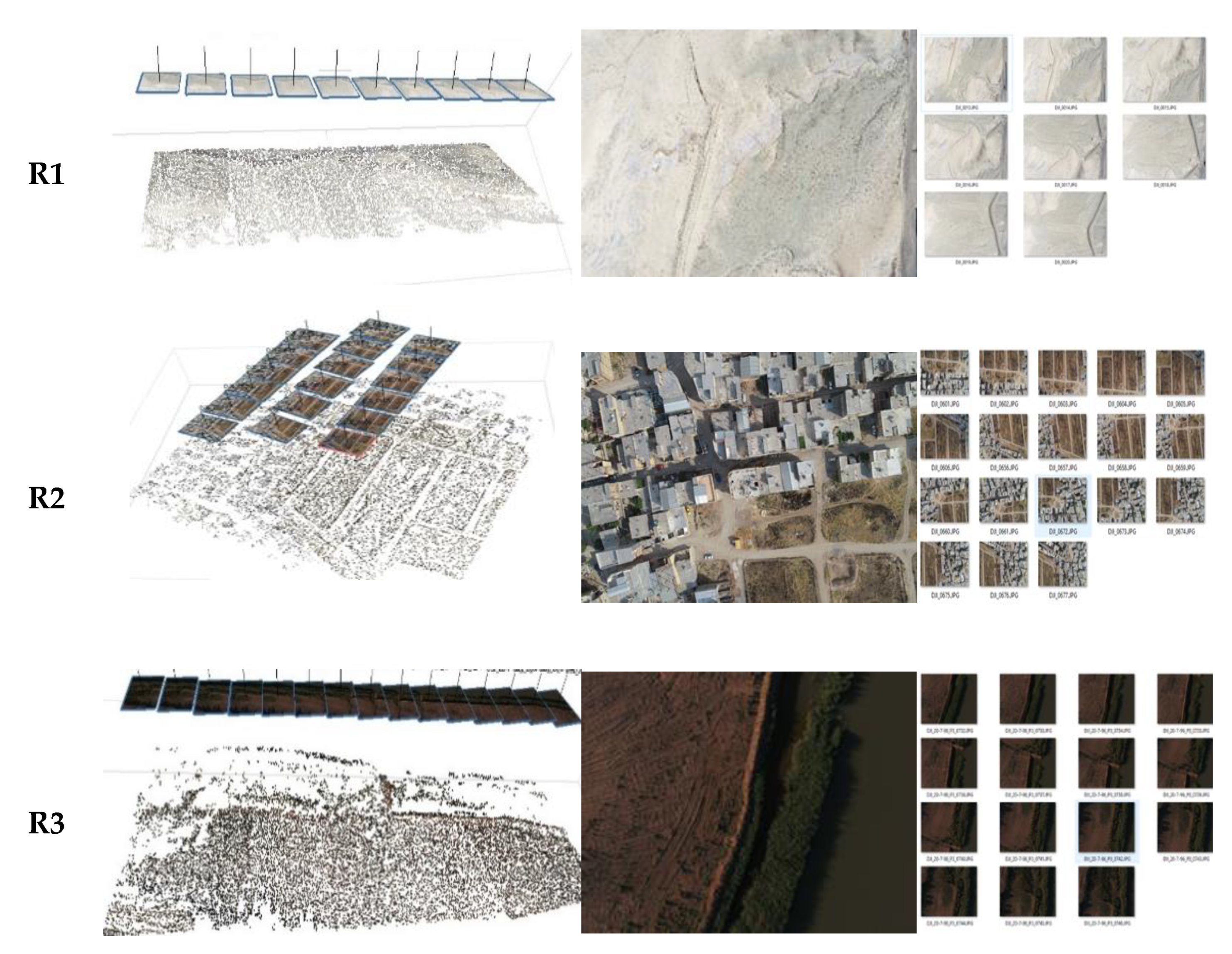
Three UAV image blocks were used in the real image network dataset. The selected images were captured by low-cost aircraft and cover both urban and rural areas with different patterns of texture. Datasets are characterized by different image resolution, the number of images, the overlap of images, changes in illumination and surfaces with different textures and sizes. Figure 5 shows the datasets used with their sample images and camera networks, and

Table 2. Specifications of the real image datasets.

Dataset	No. of Images	Camera Model	Sensor Size (mm)	Resolution (pixel)	Pixel Size (µm)	Nominal Focal Length (mm)
R1	8	DJI FC6310	13.2 × 8.8	5472 × 3648	2.41	8.8
R2	18	DJI FC6310	13.2 × 8.8	5472 × 3648	2.41	8.8
R3	15	DJI FC6520	13 × 17.3	5280 × 3956	3.28	12

summarizes their specifications.

5. Results

This section presents the evaluation results of keypoint selection methods using synthetic and real image datasets (Section 4). In the first part, the effect of selection methods is thoroughly evaluated using the SIFT detector on the synthetic dataset (Section 5.1). In the following, the results obtained using the detectors MSER, SURF and BRISK are shown in a way similar to that of SIFT. In the second part, the results of the evaluations carried out using the real image datasets are presented (Section 5.2). It should be noted that in Figure 6, Figure 7, Figure 8, Figure 9 and Figure 10 the figures shown on the left are obtained using S1 images and those on the right using the S2 images.

5.1. Matching Results Obtained Using the Synthetic Dataset

This section explains the comparative results of the experiments, including repeatability, recall, precision and spatial distribution quality for the three keypoint selection strategies.

Before presenting the results and discussions in the following sections, a sample evaluation is described to illustrate how the results in the following sections are obtained. Figure 6 shows the selected keypoint using the entropy selection criterion, the spatial saliency and the texture coefficient of one of the image pairs in the dataset. A synthetic rotation angle equal to 5° was applied to the reference image to generate geometric differences between the image pairs. Initial keypoints were extracted using SIFT for each image. The keypoints are shown in red. As can be seen, the selected keypoints for the different selection strategies are shown in green. The final matched keypoints are also shown in yellow. Generally, each selection strategy chooses different keypoint subsets with different properties, with a relatively small overlap between the results. The number of keypoints initially extracted in the reference image and the transformed image is 688 and 820, respectively. The keypoint method of selection of entropy, spatial saliency and texture coefficient reduces these numbers to 360,270 and 430 for the reference image and 440,350 and 530 for the transformed one. These numbers show that between 39% and 62% of the initial keypoints are discarded during the selection process, but matching results are not degraded at all.

5.1.1. Repeatability

The comparative results for repeatability of the SIFT detector using different keypoint reduction methods are shown in Figure 7. As shown, the repeatability of the selected keypoints is not significantly degraded by screening strategies compared to the original SIFT. Generally speaking, SIFT-Saliency with average repeatability of 65% has the best performance. SIFT-texture coefficient and SIFT-entropy are ranked second and third with 62% and 56% repeatability, respectively. SIFT-entropy has the lowest repeatability in the experiments conducted.

The results obtained for repeatability tests on images with different scales (Figure 7b) show that the SIFT texture coefficient with an average repeatability increase of 10% has superior results. SIFT-saliency results indicate that as the scale difference between images increases, the number of salient keypoints decreases significantly. This problem affects the repeatability of the selected keypoints. The aggregation of salient objects in a small part of the image is the main reason for this.

As Figure 7c shows, the repeatability of the SIFT detector degrades significantly with an increase in viewpoint angle. Repeatability of screening methods under different viewing angles is reduced by 5% for the image (S1), while in the image (S2), the keypoint selection strategies are superior in comparison to the original SIFT. SIFT-saliency obtains an average repeatability of 35% in the image (S2) and SIFT-entropy obtains 37% of the repeatable keypoints. The weakest results in this regard belong to SIFT-texture coefficient.

From the repeatability tests performed in the synthetic dataset it can be concluded that in spite of keypoint elimination, the repeatability of the selection strategies is reduced by an average of 10% to 15%. As a result, it seems losing the keypoints repeatability is not big enough to be a serious challenge in keypoint reduction strategies. Overall, the SIFT-saliency has the best performance in terms of repeatability results except for scale transformation in low-quality texture images. The SIFT-texture coefficient performs well in rotation and scale transformation but is not successful under viewpoint transformations. SIFT-entropy has the weakest results regarding repeatability quality measures in all experiments.

5.1.2. Precision

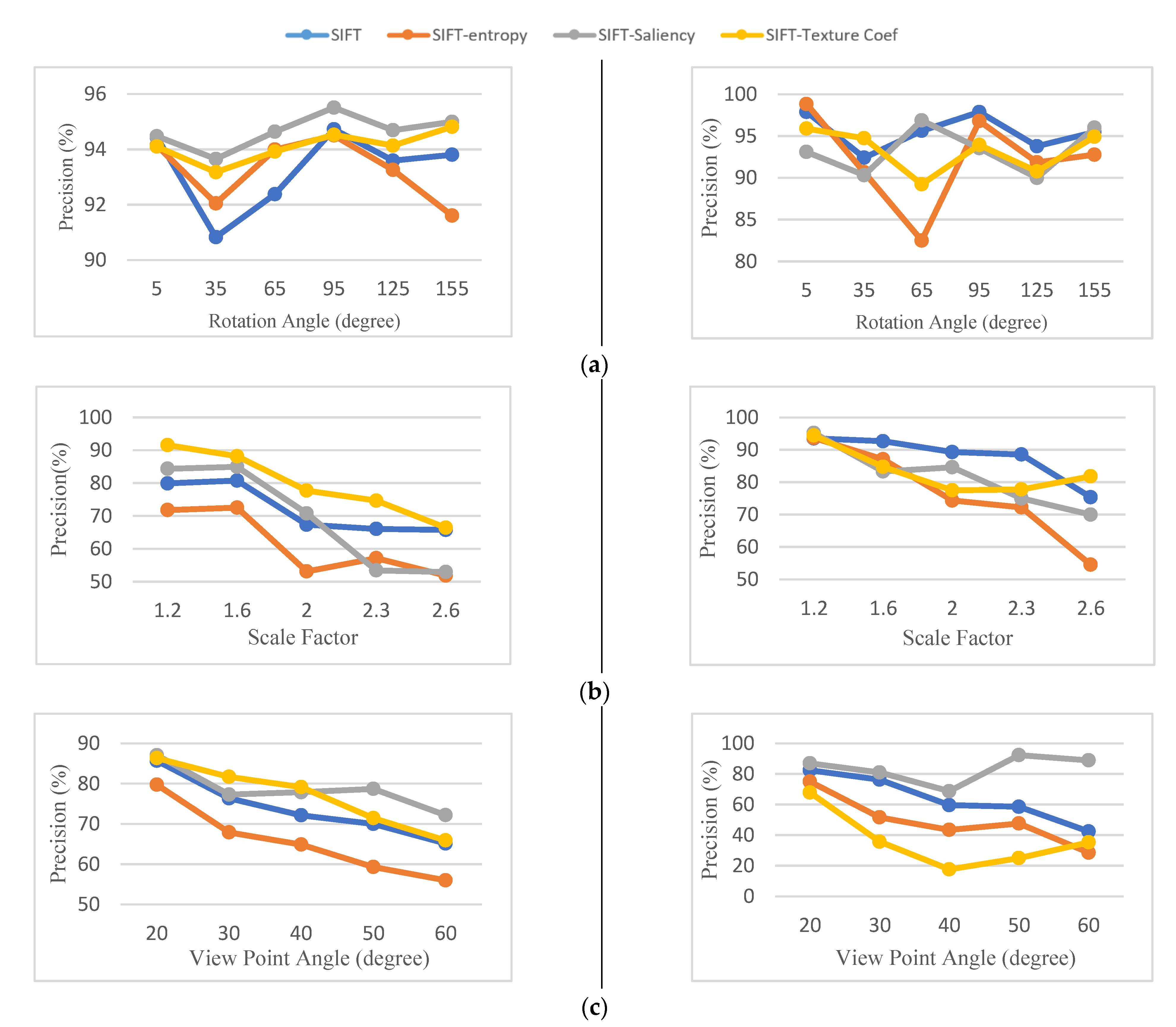
The precision of the matching results for all transformations is shown in Figure 8. The results of Figure 8a indicate that the original SIFT detector and screening methods are almost invariant with rotational changes. Selecting keypoints on the basis of their saliency increases the precision performance of SIFT in S1 dataset. SIFT-saliency with an average precision of 96.4% has superior results in the (S1) dataset. However, the SIFT-texture coefficient and the SIFT-entropy perform differently based on the scene type. Using entropy as a feature selection criterion degrades the precision of matching results in low dynamic range images (i.e., image (S2)) under rotation variations. This is mainly due to a large number of mismatches in the matching process.

As shown in Figure 8b, the matching capability of the SIFT detector and the keypoint selection methods deteriorates as the scale difference between the images increases. For the image (S1), the selection of keypoints based on the value of the texture coefficient increases the precision of the matching results. The average value of the SIFT-texture coefficient precision criteria is 85% in the image (S1). Nevertheless, none of the keypoint selection methods perform well in the image (S2). This is mainly due to the low number of extracted keypoints. However, the SIFT-entropy shows different results when the image is changed. The average precision results for SIFT-entropy are 61% for images (S1) and 76% for images (S2).

The results of Figure 8c show that SIFT-texture coefficient and SIFT-saliency improve the efficiency of the keypoint detector in terms of precision results dealing with different viewpoint images. Selected keypoints using SIFT-saliency have achieved an average precision of 78% and 83% in images (S1) and (S2), respectively. However, SIFT-texture coefficient does not perform well in (S2) dataset.

The precision results in the synthetic dataset indicate that the performance of keypoint selection methods varies depending on the image type and the applied keypoint selection criteria. Overall it can be said that the SIFT-saliency and SIFT-texture-coefficient perform better in images that contain surfaces of different textures and sizes. For the areas with poor texture quality and under viewpoint transformation, the SIFT-texture coefficient does not perform well. In all our experiments, SIFT entropy has the weakest results in terms of precision results.

5.1.3. Recall

The results of the calculation of the recall criteria for the different transformations are shown in Figure 9. As can be seen in Figure 9a, the applied selection methods outperform the original SIFT detector in all experiments. SIFT performance improves between 5% to 10% in terms of recall results using different keypoint selection methods. The SIFT-texture coefficient performs the best in images (S1) and (S2) with an average of 95%.

In most experiments for images with different scale factors and viewing angles, as shown by Figure 9b,c, the recall criterion of screening methods is relatively higher than the original SIFT. The top-ranked keypoint selection method in all transformations in the image (S1) and (S2) is SIFT-saliency with an average recall criterion of 88%, 87% and 93%, respectively.

The higher recall results in the synthetic dataset indicate that almost all of the keypoints were selected during the matching process. This means the number of redundant keypoints that are not useful in the matching process are significantly reduced by the applied selection methods.

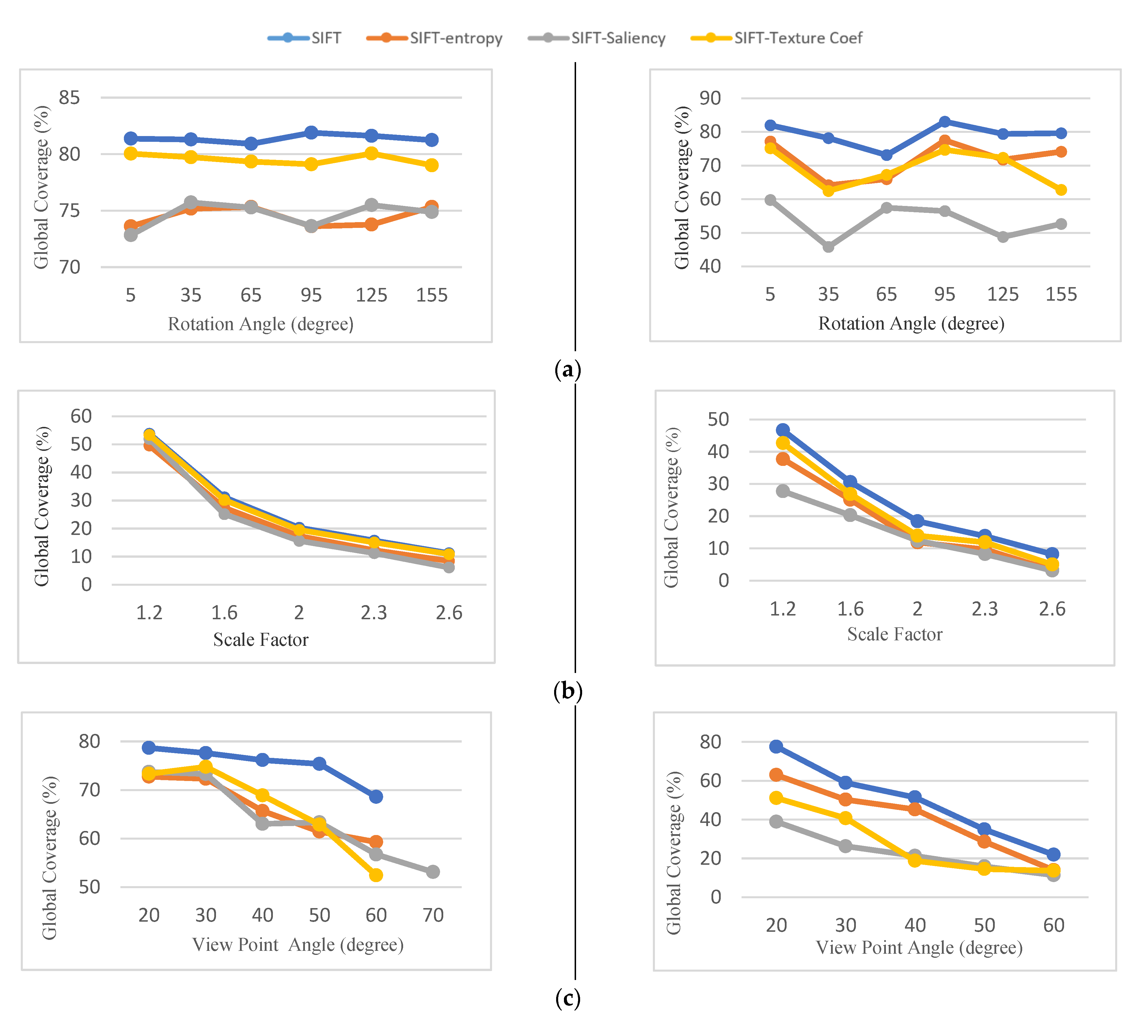
5.1.4. Global Coverage

The global coverage parameter for matching results can be seen in Figure 10. In experiments, the global coverage criterion for selected keypoints is relatively lower. As Figure 10a shows, SIFT-saliency has the lowest global coverage, with an average of 74% in the image (S1) and 53% in the image (S2). SIFT-texture coefficient has the best performance comparing keypoint discarding methods. The main reason is that the SIFT-texture coefficient method selects a higher number of keypoints during the selection process. Also, as can be seen, the screening-based version of the detectors select a subset of high-quality keypoints from the interest points that were initially extracted. However, the distribution of the selected keypoints is only reduced 5.1% to 14.41% compared to the original method.

As the scale difference between images increases, the area of Voronoi cells computed by the corresponding keypoints decreases. Consequently, the global coverage criterion is gradually reduced. This is mainly because the number of extracted keypoints decreases as the scale differences increase. As can be seen in Figure 10b, the performance of screening approaches is similar with different scale changes.

As Figure 10c shows, among the selection methods, SIFT-saliency has the weakest performance in terms of global coverage criteria, especially for the image (S2). The average global coverage criteria for SIFT-saliency for image (S1) is 63%, while the average value of this criterion is around 23.6% for image (S2). From this point of view, SIFT-entropy and SIFT-texture coefficient methods achieve similar results in the same image.

The results of global coverage in synthetic datasets indicate that, despite the keypoint selection approaches having better performance in terms of precision and recall values, the distribution of the selected keypoints cannot be controlled during the selection process and must be considered.

5.1.5. Matching Results in Detectors Other Than SIFT

Three other keypoint detectors, including MSER, SURF and BRISK, were analyzed to fully investigate the performance of keypoint selection methods. The matching results of these detectors are shown in

Table 3. The matching results of MSER detector in synthetic images.

		Rotation				Scale				Viewpoint Change
		MSER	MSER-Entropy	MSER-Saliency	MSER -Texture Coef.	MSER	MSER-Entropy	MSER-Saliency	MSER-Texture Coef.	MSER	MSER-Entropy	MSER-Saliency	MSER- Texture Coef.
Repeatability (%)	Mean	83.57	58.53	62.34	60.35	47.17	37.28	41.93	43.29	39.33	26.32	32.31	29.17
	Std.	6.32	11.39	14.08	8.00	19.74	19.85	18.30	18.20	2.03	2.44	3.35	3.68
Precision (%)	Mean	45.09	73.41	45.83	60.08	18.44	45.23	70.74	58.86	34.58	76.48	55.59	53.84
	Std.	11.06	10.46	23.31	20.26	14.41	23.18	12.65	13.88	7.88	8.62	13.65	12.41
Recall (%)	Mean	19.84	24.18	17.04	19.40	99.83	67.64	95.54	85.84	19.82	24.29	17.70	20.60
	Std.	0.17	8.95	11.34	13.76	0.21	17.55	5.50	7.47	0.24	5.82	8.02	6.21
Global coverage (%)	Mean	57.07	29.49	10.47	20.65	14.00	9.23	4.35	10.99	62.01	31.66	10.69	21.23
	Std.	5.01	12.94	4.40	17.45	3.43	2.68	487	1.65	7.22	15.96	7.43	9.17
RMSE (pixel)	Mean	0.72	0.71	0.75	0.72	1.39	1.27	1.414	1.413	0.70	0.74	0.56	0.64
	Std.	0.31	0.27	0.43	0.29	0.04	0.28	0.0006	0.0007	0.07	0.13	0.22	0.12

,

Table 4. The matching results of SURF detector in synthetic images.

		Rotation				Scale				Viewpoint Change
		SURF	SURF -Entropy	SURF -Saliency	SURF -Texture Coef.	SURF	SURF -Entropy	SURF -Saliency	SURF -Texture Coef.	SURF	SURF -Entropy	SURF -Saliency	SURF - Texture Coef.
Repeatability (%)	Mean	50.39	31.17	39.00	33.77	86.58	63.46	72.07	82.26	13.58	9.11	11.69	11.74
	Std.	12.65	13.71	13.07	16.39	2.69	5.24	4.83	2.02	2.04	1.33	2.35	2.79
Precision (%)	Mean	61.23	81.50	76.99	68.44	59.19	66.02	68.85	77.43	22.02	48.75	57.85	43.96
	Std.	16.72	9.00	12.68	17.54	14.34	11.27	12.97	11.87	7.47	9.28	9.96	12.19
Recall (%)	Mean	45.45	86.08	78.90	79.25	99.55	99.33	99.90	99.95	25.37	55.42	61.88	54.26
	Std.	15.83	6.62	11.39	9.39	0.39	0.80	0.12	0.07	7.65	14.39	10.02	7.82
Global coverage (%)	Mean	81.56	80.39	34.95	62.89	25.56	21.47	11.10	21.67	35.27	44.83	31.01	39.62
	Std.	3.98	2.01	1.39	14.43	15.62	14.78	8.27	14.41	11.39	10.31	4.39	13.47
RMSE (pixel)	Mean	0.56	0.62	0.63	0.56	1.39	1.37	1.40	1.410	0.64	0.72	0.71	0.71
	Std.	0.13	0.14	0.13	0.10	0.01	0.011	0.013	0.002	0.03	0.04	0.03	0.06

and

Table 5. The matching results of BRISK detector in synthetic images.

		Rotation				Scale				Viewpoint Change
		BRISK	BRISK -Entropy	BRISK -Saliency	BRISK -Texture Coef.	BRISK	BRISK -Entropy	BRISK -Saliency	BRISK -Texture Oef.	BRISK	BRISK -Entropy	BRISK -Saliency	BRISK - Texture Coef.
Repeatability (%)	Mean	74.12	50.51	60.77	56.73	91.89	75.89	76.67	81.76	29.42	25.30	17.43	25.23
	Std.	5.05	8.23	7.10	5.79	2.07	3.46	4.78	3.97	0.93	1.62	1.89	0.93
Precision (%)	Mean	72.09	71.53	78.22	71.77	71.74	62.04	54.40	67.66	51.09	56.11	62.60	51.75
	Std.	11.96	9.00	8.05	10.39	10.55	11.26	15.76	10.86	10.74	8.78	7.18	9.40
Recall (%)	Mean	41.87	50.96	52.16	51.58	94.73	90.07	90.97	93.65	23.63	37.71	42.43	35.77
	Std.	16.49	12.79	13.51	14.02	1.70	4.36	4.84	3.04	6.23	9.66	10.16	9.61
Global coverage (%)	Mean	71.91	57.24	30.89	58.48	24.25	17.64	9.75	18.09	40.36	32.78	16.73	31.53
	Std.	5.04	6.13	2.04	4.64	14.28	9.90	6.93	10.08	11.49	8.27	5.70	9.78
RMSE (pixel)	Mean	0.40	0.46	0.45	0.44	1.397	1.380	1.382	1.392	0.44	0.50	0.50	0.48
	Std.	0.03	0.05	0.05	0.05	0.002	0.005	0.007	0.004	0.04	0.05	0.05	0.06

and the best results are shown in Bold font. The mean and standard deviations under different geometric transformations were calculated for each assessment criterion. The higher standard deviation results of the image detectors show their different performance. Further discussion is provided in this section.

MSER

The matching results with the MSER detector are shown in Table 3, and the best results are shown in Bold font. By comparing the achieved results under different geometric transformations, it can be seen that MSER extracts the most repeatable keypoints but does not perform well in the matching process. In all experiments, the precision and stability of the obtained results in original MSER detector was lower than the keypoint selection methods. Generally speaking, keypoint selection methods achieved better results compared to the original MSER in all experiments. MSER-entropy with an average precision of 73.41% and an average recall of 24.18% outperforms other keypoint selection methods in images with varying rotation changes. For scaled images, MSER-saliency achieves superior results with average precision and recall criteria of 70.74% and 95.5%, respectively. In viewpoint change transformation, MSER-entropy gets the best results in terms of precision but considering recall parameter, MSER-saliency is the best.

SURF

The matching results using the SURF detector are summarized in Table 4. The original SURF has the best repeatability criteria results. SURF-entropy with an average precision of 81.5% and an average recall of 86% improves the matching capabilities of the detectors. SURF-texture coefficient with an average precision of 77.43% outperforms other keypoint selection algorithms dealing with images with different scale factors. SURF-Saliency with precision of 68.85% and a recall of 99.9% obtains the best results during the matching process in synthetic images with different viewing angles. In all tests, the original SURF has the best results in terms of the global coverage criterion.

BRISK

The matching results using the BRISK detector are shown in Table 5. BRISK gives greater robustness to large-scale changes. It improves matching performance over large-scale changes with an average precision of 71.74% and an average recall rate of 94.73%. Additionally, selecting keypoints based on their saliency measure increases the precision criteria around 9% and the recall criteria around 15%. Concerning the RMSE point of view, BRISK and BRISK-entropy have the best performance. In all tests, the original BRISK has the best results in terms of the global coverage criterion.

5.2. Results Obtained Using Real Images

In this section, keypoint selecting strategies were applied to blocks of real images to evaluate the effect of keypoint selection algorithms. To do so, each algorithm was performed separately on the actual image datasets. Following the pairwise matching process, the results achieved after the bundle solution were compared to the original SfM pipeline. The SIFT detector was selected for the extraction and description of the keypoints.

As the experiments on synthetic image pairs have shown, the number and distribution of extracted keypoints are decreased using keypoint selection methods. This can lead to either orientation failure due to the inadequate number of tie points or incorrect orientation results. Experiments in this section evaluate the impact of keypoint selection algorithms based on the results of the image orientation. The four criteria, as described in Section 3.3, are evaluated in the comparisons. Detailed findings will be discussed below.

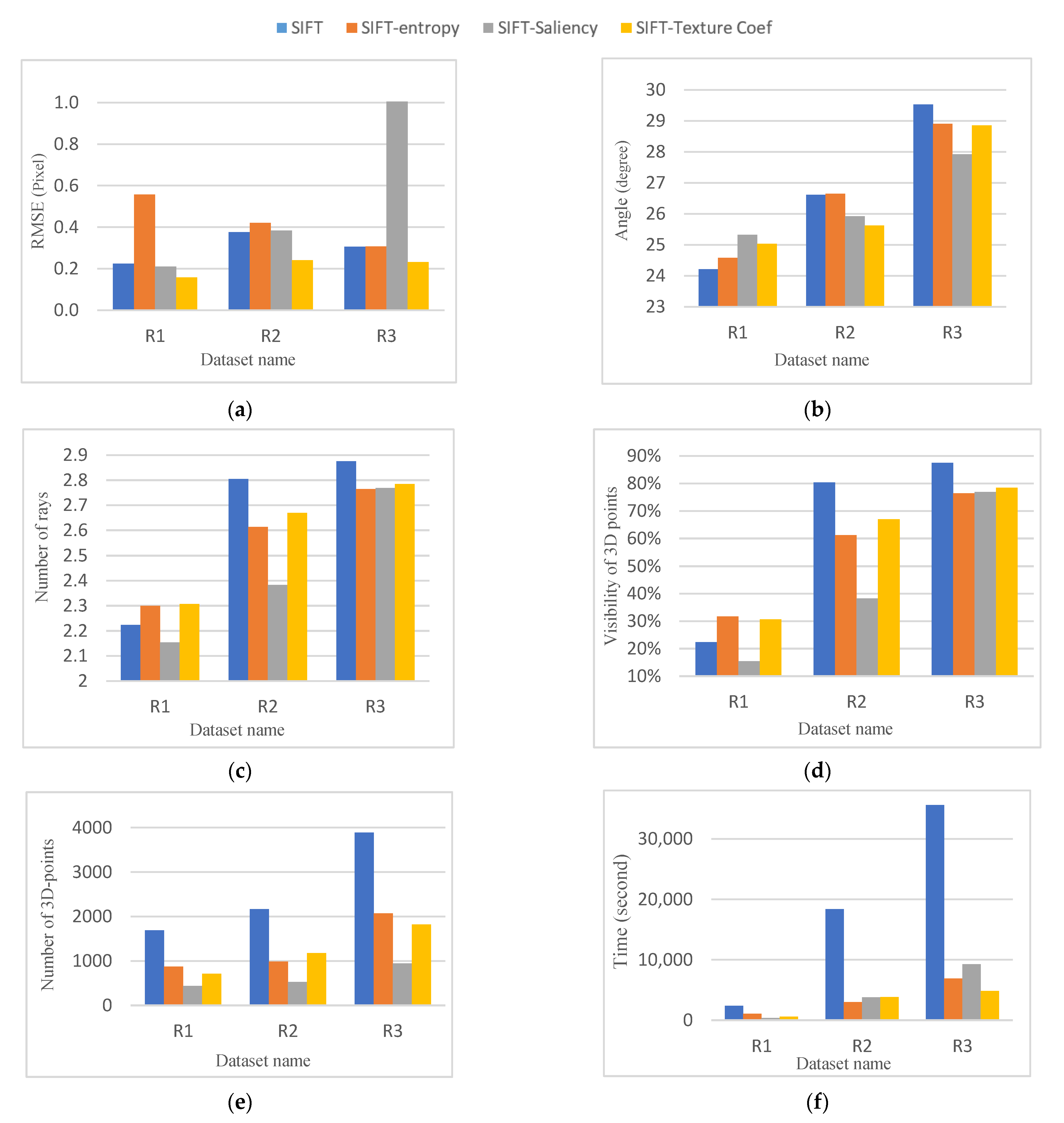
5.2.1. RMSE of the Bundle Adjustment

The re-projection error of all computed 3D points is shown in Figure 11a for all datasets. As shown, the SIFT-texture coefficient has the best performance comparing keypoint screening methods in each dataset. SIFT-saliency with 1-pixel re-projection error has the weakest test results. The main reason for this is that the R3 dataset contains uniform and low-contrast images with a lower number of salient objects. For this reason, keypoints with larger scales are selected in a saliency-based strategy, leading to lower spatial resolution. The same is true for SIFT-entropy screening in the R1 dataset. The selected keypoints in SIFT-entropy algorithm are from a larger scale, leading to larger re-projection errors in the bundle adjustment.

5.2.2. Average Angles of Intersection

Since 3D points are calculated by triangulation, a higher angle of intersection of similar rays provides more accurate 3D details. As shown in Figure 11b, higher intersection angles are achieved in R1 and R2 datasets consisting of higher overlapping images (almost more than 70%). For R1 datasets with fewer overlapping images, the intersection angles are relatively smaller. In this respect, however, SIFT saliency performs better.

5.2.3. Average Rays Per 3D Point

As the overlap between images in a dataset increases, more redundancy was expected for 3D object coordinates. As shown in Figure 11c, higher average multiplicity for the tie-points is achieved in datasets R1 and R2 with higher overlapping images. The larger multiplicity belongs to the original SIFT and SIFT-texture coefficient keypoints with an average of 2.83 and 2.72 rays, respectively. However, for R1 datasets containing fewer overlapping images, SIFT-entropy and SIFT-texture coefficients with an average ray of 2.3 outperform other methods.

5.2.4. Visibility of 3D Points in More Than Three Frames

Figure 11d shows the visibility of the 3D points that are normalized with respect to all extracted points for each dataset. The visibility results indicate that 30% of the triangulate points using the SIFT-entropy strategy are visible in three images in the R1 dataset. The original SIFT and SIFT-texture coefficient strategies achieved the best results for R2 and R3 datasets with an average image overlap of 60% and 80%.

5.2.5. The Number of 3D Points

Figure 11e shows the number of the 3D points used for the bundle adjustment process. The results indicate that nearly 50% of the 3D points are eliminated using the SIFT-entropy and SIFT-texture coefficient strategies. The SIFT-saliency method reduces nearly 75% of 3D points compared to the original SIFT. However, the quality of the image orientation is not reduced except for the R3 dataset. This is because it contains a relatively lower number of salient objects.

5.2.6. Processing Time

The time required for the orientation of the image for each dataset is shown in Figure 11f. As shown, using the original SIFT in blocks with a large number of images is more time-consuming. Whereas selection-based approaches are more efficient, SIFT-saliency, SIFT-entropy and SIFT-texture coefficient keypoint selection approaches are the most time-efficient strategies for R1, R2 and R3 datasets.

6. Discussions

The presented evaluation framework (Section 5) compares results in two separate phases. In the first part, the evaluation process is performed at the end of the descriptor matching phase using synthetic datasets. The tests then compare the results of a real image block orientation to understand the performance of keypoint selection methods for 3D reconstruction purposes. The achieved results are respectively discussed in this section.

The achieved results on the synthetic dataset show that the repeatability of the selected keypoints is 10% to 15% degraded by keypoint selection strategies when SIFT detector is applied to extract keypoints. Similarly, repeatability of the selected keypoints is 3% to 20% lower when keypoints are extracted using MSER, SURF and BRISK detectors.

From the precision point of view, the performance of the applied screening methods was different depending on the image type and the keypoint selection criteria. Generally, in most experimental cases, precision was improved 10% to 15%. Furthermore, SIFT performance improves between 5% to 10% in terms of recall results using different keypoint selection methods. For the MSER detector, in all experiments the precision and recall of the obtained results in the original MSER detector was lower than the screening methods. Generally speaking, keypoint selection methods achieved 25% to 40% better precision results compared to the original MSER in the conducted experiments. Keypoint selection methods in the SURF detector had similar performance, enhancing the precision and recall results from 10% to 25% in synthetic dataset. Selecting keypoints based on their saliency measure increases the matching capability of the BRISK detector. Precision and recall criteria for both rotation and viewpoint change tests are improved in the BRISK detector. However, the selection of keypoints based on selection criteria measures does not affect the performance of the BRISK detector in scaled images.

The result of global coverage criteria for all detectors shows that the global coverage criterion for selected keypoints is relatively lower and should be considered.

Experiments on synthetic image pairs showed that screening methods decrease the number and distribution of selected keypoints. Further experiments were performed to evaluate the impact of these shortcomings on the results of the 3D reconstruction. Similar to synthetic dataset, the achieved results showed that screening methods perform well in real images. The re-projection error of computed 3D points is on average 15% to 30% decreased using selected keypoints. This means that the adequate number of tie points with an appropriate distribution are selected by screening methods. However, the keypoint selection strategies are not capable of controlling the scale of the selected keypoints. As a result, keypoints with larger scales may be selected, which leads to less accurate results in bundle adjustment. As far as computing time is concerned, keypoint selection approaches outperform conventional methods and improve time efficiency, especially for blocks with large number images.

7. Development of a New Hybrid Keypoint Selection Algorithm

As shown by the presented results on real and synthetic images (Section 5), keypoint selection methods, thanks to their own specifications and functionalities, have an overall positive impact on the accuracy of image matching and orientation. Each of the keypoint reduction methods discussed perform well when they are separately applied for keypoint selection. However, developing a hybrid keypoint selection algorithm that combines all these criteria simultaneously could be a more efficient solution. This is because it can provide the opportunity to compensate for the shortcomings of each keypoint selection criteria and, and thus, reinforce their strengths. On this basis, in this section, a new hybrid keypoint selection algorithm is proposed, which uses all the keypoint selection criteria at the same time.

In order to combine entropy, saliency and texture coefficient criteria to achieve a single competency value for each keypoint, a simple average ranking method is used. Suppose that $n$ initial keypoints are extracted, and each criterion of entropy, saliency and texture coefficient are computed for them. For each quality measures, the rank vector is computed as follows:

$$R_i=\left\{r_i^j\right\}j=\mathrm{1.2.3}i=\mathrm{1.2.}\dots n,$$

(11)

where $r_i^j$ represent the rank of ith keypoint in the jth quality measures. The rank of each keypoint in each quality criteria is calculated by sorting the quality measures values in descending order and assigning the rank according to its position.

Afterwards, the average rank for each keypoint (${\overline{r}}_i$) is computed using the following equation:

$${\overline{r}}_i=\frac{\left({{\displaystyle \sum }}_j^n{r}_i^j\right)}{n}$$

(12)

where n is the number of criteria and ${\overline{r}}_i$ is the average rank for the ith keypoint. Once the average rank for each keypoint is computed, the image is gridded and the keypoints with ${\overline{r}}_i$ larger than the average rank of each cell is selected as the final keypoints.

To evaluate the proposed hybrid criterion, different experiments are carried out similar to those mentioned in Section 5.2. To this end, the real datasets of R1, R2 and R3 (Section 4) were used to assess the results of the image orientation. The four quality measures mentioned in Section 3.3, including re-projection error of bundle adjustment, average rays per 3D points, visibility of 3D points in more than three images and average intersection angle per each 3D point are used to compare the performance of the proposed algorithm to that of SIFT. The required processing time is also tested to evaluate the time efficiency of the proposed method. Detailed results are discussed below.

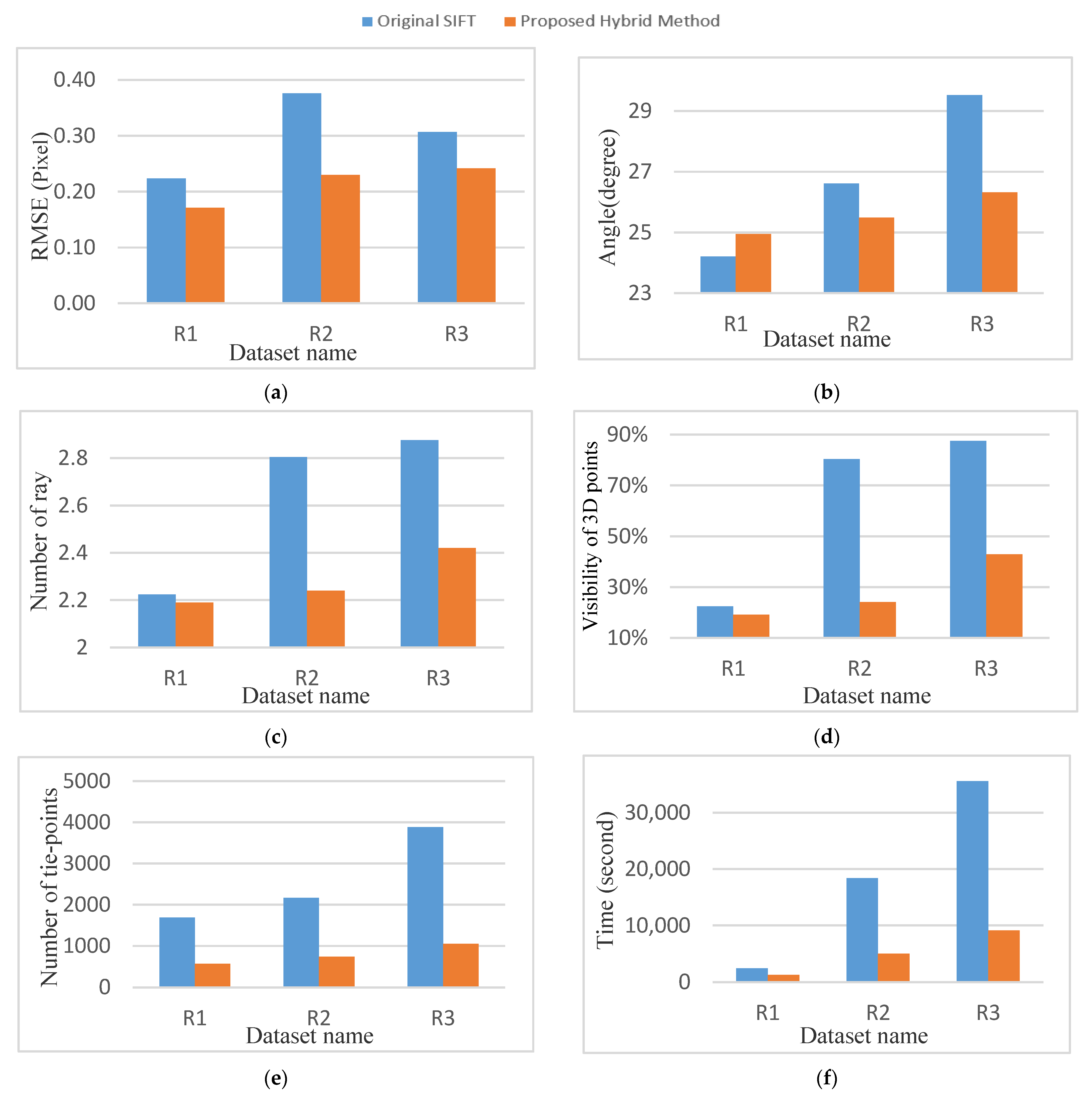
7.1. RMSE of the Bundle Adjustment

Figure 12a shows the RMSE of bundle adjustment in the hybrid proposed method and the original SIFT. The re-projection error of bundle adjustment for the proposed hybrid method is lower in all datasets. The re-projection error is on average 22% to 40% improved using the proposed hybrid algorithm.

7.2. Average Angles of Intersection

The average intersection angles in the proposed algorithm, as shown in Figure 12b, for dataset R2 and R3 are relatively smaller. For R1 datasets with fewer overlapping images, the average intersection angle for the proposed method is 3% larger in comparison to the original SIFT.

7.3. Average Rays Per 3D Point

The average multiplicity results are shown in Figure 12c and indicate that the proposed algorithm does not perform well from this aspect. For the R1 dataset, the average multiplicity for the tie-points for both the proposed method and the original SIFT is almost the same. However, for R2 and R3 dataset, the average multiplicity for the proposed method is 15% to 20% lower in comparison with the original SIFT.

7.4. Visibility of 3D Points in More Than Three Frames

The visibility of the 3D points is shown in Figure 12d, which are normalized with respect to all extracted points for each dataset. The visibility results indicate that in the R1 dataset for both the original SIFT and the proposed method, an average of 20% of the triangulate points are visible in more than three images. The visibility results in the proposed method and original SIFT differ 54% and 45% for R2 and R3 datasets, respectively.

7.5. The Number of 3D points

Figure 12e shows the number of the 3D points applied for the bundle adjustment process. A high number of keypoints are eliminated during keypoint selection. Generally, the proposed method eliminates averagely 70% of keypoints which leads to lower multiplicity and average rays per 3D point. However, the quality of the bundle adjustment is not reduced in comparison with the original SIFT.

7.6. Processing Time

The required processing time for the image orientation for each dataset is shown in Figure 12f. Similar to the results of Section 5.2.6, the proposed method is more efficient regarding the required processing time.

The evaluation results of the proposed method show that applying all the discussed criteria simultaneously for keypoint selection could provide better results regarding matching and 3D reconstruction results. The proposed algorithm enhances the performance of bundle adjustment in terms of re-projection error and processing time. However, the problem of setting the optimal threshold for keypoint selection/discarding is still a challenge. As shown by the experiments, a high number of keypoints are eliminated during keypoint selection which leads to lower performance in terms of multiplicity and average rays per each 3D point. Furthermore, despite the obtained results in Section 5.2, the problem of image scene type, which affected the results of the R3 dataset is solved by the combination of selection criteria.

8. Conclusions

Accurate keypoint extraction and matching is a key issue for various UAV photogrammetry applications. Previous studies have not paid due attention to the impact of the information content criteria on the quality of the selected keypoints. Several tests were carried out in this paper using simulated and real data to verify the impact of different information content criteria on keypoint selection tasks. To this end, three strategies have been chosen to select among the detected interest points. In these approaches, different quality measures were applied to the conventional keypoint detectors and extracted keypoints were selected based on their measure values. In summary, the following results have been obtained.

• Each keypoint detector performs differently depending on the type of image and the type of scene. Enhancing the capabilities of the original detectors, keypoint selection strategies (i.e., entropy, saliency and texture coefficient), are advantageous for accurate image matching and UAV image orientation.
• Despite the reduction of keypoints, the keypoint selection strategies applied almost preserve the distribution of corresponding points.
• Information-based selection methods can effectively control the number of keypoints detected. As discussed (Section 5.1 and Section 5.2.5), in our experiments, the remaining keypoints range between 38% to 61% for the synthetic data and between 25% to 50% for the real data. As a result, the large number of detected keypoints that make the matching process time-consuming and error-prone is significantly decreased. The results of the image orientation also confirm this fact.
• It should be noted that keypoint selection algorithms are not capable of finding matched pairs with lower scale over entire image. This is because there is a lack of control over the scale of the keypoints in the selection process.

It can generally be concluded that keypoint selection methods have a positive impact on the accuracy of image matching. Developing an approach that uses all the keypoint selection criteria simultaneously is, therefore, of interest. To this end, a new hybrid keypoint selection that combines all of the information content criteria discussed in this paper was proposed. The results from this new screening method were also compared with those of SIFT, which showed a 22% to 40% improvement for the bundle adjustment of UAV images. In addition, providing a strategy that considers the scale of keypoints is also suggested for further research. Last but not least, it is possible to use measures other than a criterion’s average as the threshold, below which the keypoints are discarded. This is done to study the effect of new thresholds on the quality of point selection. Therefore, it is suggested that this issue is further explored in future studies.