Wide Sliding Window and Subsampling Network for Hyperspectral Image Classification

Abstract

Recently, deep learning methods, for example, convolutional neural networks (CNNs), have achieved high performance in hyperspectral image (HSI) classification. The limited training samples of HSI images make it hard to use deep learning methods with many layers and a large number of convolutional kernels as in large scale imagery tasks, and CNN-based methods usually need long training time. In this paper, we present a wide sliding window and subsampling network (WSWS Net) for HSI classification. It is based on layers of transform kernels with sliding windows and subsampling (WSWS). It can be extended in the wide direction to learn both spatial and spectral features more efficiently. The learned features are subsampled to reduce computational loads and to reduce memorization. Thus, layers of WSWS can learn higher level spatial and spectral features efficiently, and the proposed network can be trained easily by only computing linear weights with least squares. The experimental results show that the WSWS Net achieves excellent performance with different hyperspectral remotes sensing datasets compared with other shallow and deep learning methods. The effects of ratio of training samples, the sizes of image patches, and the visualization of features in WSWS layers are presented.

1. Introduction

Hyperspectral images (HSI) include hundreds of continuous spectral bands, which gives them abundant information to classify different ground objects. These images, together with the classification methods, are used in many applications including agriculture monitoring, change detection of land cover, urban mapping, forest protection, and object detection. One difficulty for HSI classification involves homogeneous ground objects having different spectral features due to different illumination, atmospheric environment, etc. during imaging process. Another difficulty is that although a large number of spectral bands provide a large amount of data, the training data are usually very limited and the image scene is complicated because of mixed pixels.

In the past decades, researchers used different machine learning methods for HSI classification including k-nearest neighbors (KNN) [1], support vector machine (SVM) [2], multilayer perceptron (MLP) [3], random forest (RF) [4], radial basis function network (RBF) [3], etc. These methods are mainly in the spectral domain.

Recently, many works utilizing both spectral and spatial features have been proposed to obtain higher HSI classification performance including the morphological profiles (MPs) [5], Markov random fields (MRFs) [6], SVM-MRF [2], sparsity-based method [7] using spatial and contextual features, and generalized composite kernel machine [8], which tries to balance spectral and spatial information without introducing weights and parameters. These methods usually combine both the spectral and spatial information from the neighborhood area of the given pixel.

With deep learning, many methods based on convolutional neural network (CNN) have been proposed to learn features automatically in both spacial and spectral domains [9,10,11,12,13,14,15]. This is a great advantage compared with the aforementioned methods which use manually extracted features from only the spatial domain or both the spatial and spectral domains. Zhang et al. [16] gave a full description of how to use deep learning methods with different types of inputs and applications. A contextual deep CNN was proposed by Lee et al. [9], which can optimally find local contextual interactions by exploiting local spatio-spectral relationships of neighboring pixels. Mei et al. [10] proposed a CNN with five layers combining advances of batch normalization, dropout, and parametric rectified linear unit (PReLU) activation function. Gao et al. [11] proposed a CNN with various features extracted from the input images. Wang et al. [12] proposed an end-to-end fast dense spectral–spatial convolution (FDSSC) method, which uses different convolutional kernels to extract both spectral and spatial features. Paoletti et al. [13] proposed a 3-D CNN that uses both spectral and spatial information. A diverse region-based CNN was proposed by Zhang et al. [14], which encodes semantic context-aware representation to obtain more valuable features. Chen et al. [15] proposed a method to extract hierarchical deep spatial features from CNN. Other deep architectures have also been explored for hyperspectral image classification. Mou et al. [17] presented a deep recurrent neural network to do hyperspectral image classification. Spectral-spatial attention networks based on RNN and CNN were proposed by Mei et al. [18], which can learn spectral correlations within a continuous spectrum and spatial relevance within neighboring pixels.

CNN was combined with other recently emerged methods to solve the HSI classification problem. The hybrid spectral CNN (HybridSN) [19] and mixed CNN [20] are spectral–spatial 3-D CNNs followed by spatial 2-D CNNs. Gong [21] proposed multiscale convolution (MS-CNNs) with diversified metric to obtain discriminative features. CNN was also combined with active learning [22,23] to obtain good classification performance with few training labels. Feng et al. [24] combined attentional mechanism, adaptive region search, and multibranch CNN to learn features more flexibly. Chen et al. [25] designed automatic CNN to find deep learning architecture automatically for HSI classification. Hong et al. [26] proposed invariant attribute profiles (IAPs) to extract the spatial invariant features. Wang et al. [27] combined adaptive dropBlock-Enhanced and generative adversarial networks (GAN) for HSI classification. A deep fully convolutional network (FCN) with an efficient nonlocal module (ENL-FCN) was proposed by Shen et al. [28] for HSI classification. A content-guided CNN (CGCNN) proposed by Liu et al. [29] adjusts the kernel shape adaptively according to the spatial distribution of land covers. Tang et al. [30] proposed a 3-D octave convolution with the spatial–spectral attention network (3DOC-SSAN) to capture discriminative spatial–spectral features. Masarczyk et al. [31] proposed a strategy of transfer learning that uses unsupervised pretraining step and combined it with CNN.

Although the deep learning methods have made great improvements in various areas, they usually need a long training time because of the large number of parameters. Another problem is that CNN achieves greater performance as the depth increases. However, the training samples of HSI images are usually limited in number, and small patches are used for HSI classification to extract spatial features. Therefore, it is not possible to use CNN with many layers and a large number of convolutional kernels. Different learning models have been proposed to gain better performance. Okwuashi et al. [32] proposed a deep support vector machine (DSVM) for hyperspectral image classification. Cao et al. [33] proposed a cascaded dual-scale crossover network, which extracts more features without making the network deeper. Recently, many works on wide learning [34,35], as well as wide and deep learning architectures [36], have been proposed. Here, width means the number of hidden neurons or channels in the fully connected or convolutional layers. The wide fully connected neural networks are equivalent to a Gaussian process. Therefore, training and learning can be characterized simply by evaluating the Gaussian process, and it is found that the wide neural network generalizes better [34,35]. Other than Gaussian kernels, Daniel et al. [37] proposed harmonic networks, which use circular harmonics instead of CNN kernels. Liu et al. [38] extended it, and proposed naive Gabor networks to reduce the number of parameters involved in HSI classification. Different hyperspectral classification methods have been summarized in Table 1.

Table 1. Hyperspectral classification methods.

Types and Descriptions	Related Works
Machine learning, spectral features	KNN [1], SVM [2], MLP [3], RBF [3], RF [4]
Machine learning and other methods without using deep learning, spectral, and spatial features	MPs (Fauvel et al.) [5], IAPs (Hong et al.) [26], MRFs (Li et al.) [6], SVM-MRF (Tarabalka) [2], sparsity-based method (Chen et al.) [7], generalized composite kernel machine (Li et al.) [8]
Deep learning, spectral, and spatial features	contextual CNN (Lee et al.) [9], Mei et al. [10], Gao et al. [11], FDSSC (Wang et al.) [12], 3-D CNN (Paoletti et al.) [13], diverse region-based CNN (Zhang et al.) [14], Chen et al. [15], Zhang et al. [16], deep RNN (Mou et al.) [17], Mei et al. [18]
Deep learning combined with emerging methods, spectral, and spatial features	HybridSN (Roy et al.) [19], mixed CNN (Zheng et al.) [20], CNN with active learning: (Haut et al.) [22], and (Cao et al.) [23], attentional model (Feng et al.) [24], MS-CNNs (Gong et al.) [21], automatic CNN (Chen et al.) [25], dropBlock GAN (Wang et al.) [27], ENL-FCN (Shen et al.) [28], CGCNN (Liu et al.) [29], 3DOC-SSAN (Tang et al.) [30], transfer learning (Masarczyk et al.) [31]
Learning models with different novel architectures, spectral, and spatial features	DSVM (Okwuashi et al.) [32], cascaded dual-scale crossover network (Cao et al.) [33], naive Gabor networks(Liu et al.) [38]

In this paper, we propose a wide sliding window and subsampling network (WSWS Net) for hyperspectral image classification. It is based on transform kernels with sliding windows, which can be extended in the wide direction to learn both spatial and spectral features sufficiently. Sorting and subsampling operations are introduced to reduce the number of outputs of transform kernels. The above process is denoted as the WSWS layer. Then, succeeding WSWS layers are added in the same way, and multiple WSWS layers can be combined in cascade to learn higher level spatial and spectral features with a larger field of view. Finally, a fully connected layer with linear weights is combined with the WSWS layers to predict the pixel class. The proposed WSWS Net has the following features:

• Extracting a higher level of spatial and spectral features by the multiple layers of transform kernels efficiently, and the parameters of these transform kernels can be learned using unsupervised learning or obtained directly by randomly choosing them from training samples.
• Adjusting features easily by adjusting the width and the field of view of WSWS layers according to the size of training data.
• Training the WSWS Net easily, because the weights are mostly in the fully connected layer, which can be computed with least squares.

The rest of the paper is organized as follows. Section 2 presents the proposed WSWS Net. Section 3 discusses the used datasets and the experimental settings. Section 4 provides the HSI classification results with the proposed WSWS Net. In Section 5 and Section 6, discussions and conclusions are given.

2. Wide Sliding Window and Subsampling Network (WSWS Net)

In this section, the proposed WSWS Net is described in detail, including how to generate patch vectors from HSI as inputs to the WSWS Net; how to construct the wide transform kernel layers using sliding window, sorting, subsampling; and how to go deeper with a fully connection layer. Finally, we explain how to adjust the width of the transform kernel layers, and how to obtain different higher level spacial and spectral features by adjusting the field of view in the transform kernel layers. The architecture of the WSWS Net is shown in Figure 1.

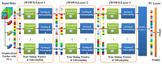
Figure 1. Architecture of the wide sliding window and subsampling (WSWS) network for hyperspcetral image classification.

2.1. Generating Patch Vectors for WSWS Net from HSI Data

The original HSI data are denoted as $\mathbf{X}\in {\mathbf{R}}^{W\times H\times B}$, where $W\times H$ is the width and height of the HSI, and B is the number of hyperspectral bands, which is usually as large as several hundred with a very large number of redundant spectral information. Therefore, principal component analysis (PCA) is often performed to reduce the number of bands to $B_{PCA}$. After that, normalization is performed for each chosen reduced band, which is as shown below.

$${\mathbf{X}}_{norm}\left(k\right)=\frac{\mathbf{X}\left(k\right)-min\left(\mathbf{X}\left(k\right)\right)}{max\left(\mathbf{X}\left(k\right)\right)-min\left(\mathbf{X}\left(k\right)\right)},1\le k\le B_{PCA}$$

(1)

Suppose there are C classes of land objects, and the generated 3-dimensional patches have the size with $S_W\times S_H\times B_{PCA}$ (odd window size in both width and height directions). Before generating patches, zero padding is performed on the whole image ${\mathbf{X}}_{norm}$ with padding sizes $\left(S_W-1\right)/\phantom{\left(S_W-1\right)2}2$ and $\left(S_W-1\right)/\phantom{\left(S_W-1\right)2}2$ in width and height directions, respectively. The HSI image after zero padding is denoted as ${\mathbf{X}}_{norm\_pad}$. The independent pixels are called instances. A given proportion of instances for each class whose numbers are denoted as $Nc\left(1\le c\le C\right)$, and 3D patches are generated for pixels of each class automatically from ${\mathbf{X}}_{norm\_pad}$ according to the required numbers of training, validation, and test processes. These patches are flattened as vectors in cascade along spectral bands, and denoted as ${\mathbf{X}}_{tr}$, ${\mathbf{X}}_{val}$, and ${\mathbf{X}}_{test}$, respectively. The length of these patch vectors is $M=S_W\times S_H\times B_{PCA}$.

2.2. Constructing the Transform Kernel Layer by Wide Sliding Window and Subsampling

The CNN uses convolutional kernels to extract spatial features with multiple channels. The local receptive field and the weight sharing are used to reduce the number of weights of convolutional kernels. Although it is reduced a lot, the weights are learned with back propagation (BP)-based training methods for a number of epochs, which is time-consuming. Another problem is that for HSI classification, small patches are usually fed as input to convolutional layers, making it difficult to use CNN with very deep architecture. Therefore, researchers started to use different kernels to improve the performance of learning models, such as circular harmonics [37] and Naive Gabor filters [38]. In the proposed WSWS Net, the transform kernels are used as extractors, and the sliding window is used to make it much wider to represent learning features. Then, the more important extracted features are obtained with sorting and subsampling processes as the important property of WSWS layers is that the parameters of these kernels can be learned by unsupervised such as k-means or EM algorithm, or they can be obtained by randomly choosing them from training instances. The constructing process of the wide sliding window and subsampling (WSWS) layers is shown in Figure 2.

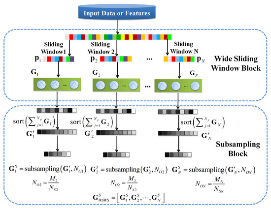
Figure 2. Constructing the wide sliding window and subsampling (WSWS) Layer by wide sliding window and subsampling.

For HSI classification, the size of the 1 dimensional sliding window is chosen as m and the number of instances is denoted as $N_p$. The sliding direction is from top to bottom. For the $n\mathrm{th}$ ($1\le n\le N=\left(M-m+1\right)$) sliding time, the input vector ${\mathbf{p}}_n\in {\mathbf{R}}^{m\times N_p}$ from $\mathbf{X}$ is fed into a set of Gaussian kernels denoted as $\{g_{n1},g_{n2},\cdots ,g_{n{M}_n}\}$, where $M_n$ denotes the number of Gaussian kernels for $n\mathrm{th}$ sliding time. The outputs of the Gaussian kernels from the $n\mathrm{th}$ sliding are denoted by

$${\mathbf{G}}_n=\left[\begin{array}{cccc}{g}_{n1}\left({\mathbf{p}}_n\right),& g_{n2}\left({\mathbf{p}}_n\right),& \dots ,& g_{n{M}_n}\left({\mathbf{p}}_n\right)\end{array}\right]$$

(2)

where $g_{ni}\left({\mathbf{p}}_n\right)(1\le i\le M_n)$ is a column vector with $N_p$ components (number of patch vectors).

During sliding, the Gaussian kernels are extended in the wide direction, where the width refers to the number of hidden units in the WSWS layer. Finally, for the input ${\mathbf{p}}_{WSWS}=\left[{\mathbf{p}}_1,{\mathbf{p}}_2,\cdots ,{\mathbf{p}}_N\right]$, a wide sliding window layer is constructed with N sets of Gaussian kernels denoted as

$${\mathbf{G}}_{WSWS}=\left[\begin{array}{cccc}{\mathbf{G}}_1,& {\mathbf{G}}_2,& \dots ,& {\mathbf{G}}_N\end{array}\right]$$

(3)

After extending it in the wide direction to obtain sufficient number of features, the outputs are sorted and subsampled to reduce the number of outputs. The sorting is performed in each set of Gaussian kernels. All the instances of each Gaussian kernel are summed and sorted from maximum to minimum, which is expressed as

$${\mathbf{I}}_{WSWS}=\left[{\mathbf{I}}_1,{\mathbf{I}}_2,\cdots ,{\mathbf{I}}_N\right]=\left[\mathrm{sort}\left({\sum }_{j=1}^{N_p}{\mathbf{G}}_1\right),\mathrm{sort}\left({\sum }_{j=1}^{N_p}{\mathbf{G}}_2\right),\cdots ,\mathrm{sort}\left({\sum }_{j=1}^{N_p}{\mathbf{G}}_N\right)\right]$$

(4)

The outputs of each set of Gaussian kernels in ${\mathbf{G}}_{WS}$ are sorted according to the sorting indices, given by

$${{\mathbf{G}}^{\prime }}_{WSWS}=\left[{{\mathbf{G}}^{\prime }}_1,{{\mathbf{G}}^{\prime }}_2,\cdots ,{{\mathbf{G}}^{\prime }}_N\right]=\left[{\mathbf{G}}_1\left({\mathbf{I}}_1\right),{\mathbf{G}}_2\left({\mathbf{I}}_2\right),\cdots ,{\mathbf{G}}_N\left({\mathbf{I}}_N\right)\right]$$

(5)

Then, they are subsampled by a given subsampling interval $N_{Sn}$. The numbers of outputs after subsampling are given by

$$N_{WSWS}=\left[N_{O1},N_{O2},\cdots ,N_{ON}\right]=\left[\frac{M_1}{N_{S1}},\frac{M_2}{N_{S2}},\cdots ,\frac{M_N}{N_{SN}}\right]$$

(6)

The final outputs after subsampling outputs are denoted by

$${\mathbf{G}}_{WSWS}^S=\left[{\mathbf{G}}_1^S,{\mathbf{G}}_2^S,\cdots ,{\mathbf{G}}_N^S\right]$$

(7)

where,

$${\mathbf{G}}_n^S=\mathrm{subsampling}\left({{\mathbf{G}}^{\prime }}_n,N_{On}\right),1\le n\le N$$

(8)

2.3. Going Deeper with a Fully Connected Layer

In order to learn higher level spatial and spectral features, the WSWS Net is extended deeper with more WSWS layers. The input of the second layer is denoted as

$${\mathbf{p}}_{WSWS}^{\left(2\right)}=\left[{\mathbf{p}}_1^{\left(2\right)},{\mathbf{p}}_2^{\left(2\right)},\cdots ,{\mathbf{p}}_{N^{\left(2\right)}}^{\left(2\right)}\right]={\mathbf{G}}_{WSWS}^{\left(1\right)S}=\left[{\mathbf{G}}_1^{\left(1\right)S},{\mathbf{G}}_2^{\left(1\right)S},\cdots {\mathbf{G}}_{N^{\left(1\right)}}^{\left(1\right)S}\right]$$

(9)

where ${\mathbf{G}}_{WSWS}^{\left(1\right)S}={\mathbf{G}}_{WSWS}^S$ is the sampled outputs of the first WSWS layer. The size of the sliding window of the second layer is $m^{\left(2\right)}$. The Gaussian kernels for the $n^{\left(2\right)}\mathrm{th}$ ($1\le n^{\left(2\right)}\le N^{\left(2\right)}=\left(M^{\left(2\right)}-m^{\left(2\right)}+1\right)$) sliding time in the second layer are set as $\{g_{n1}^{\left(2\right)},g_{n2}^{\left(2\right)},\cdots ,g_{n{M}_n^{\left(2\right)}}^{\left(2\right)}\}$, and $M_n^{\left(2\right)}$ denotes the number of Gaussian kernels for $n^{\left(2\right)}\mathrm{th}$ sliding time.

The $N^{\left(2\right)}$ sets of Gaussian kernels are denoted as

$${\mathbf{G}}_{WSWS}^{\left(2\right)}=\left[\begin{array}{cccc}{\mathbf{G}}_1^{\left(2\right)},& {\mathbf{G}}_2^{\left(2\right)},& \dots ,& {\mathbf{G}}_{N^{\left(2\right)}}^{\left(2\right)}\end{array}\right]$$

(10)

The final outputs after sampled are denoted by

$${\mathbf{G}}_{WSWS}^{\left(2\right)S}=\left[{\mathbf{G}}_1^{\left(2\right)S},{\mathbf{G}}_2^{\left(2\right)S},\cdots ,{\mathbf{G}}_{N^{\left(2\right)}}^{\left(2\right)S}\right]$$

(11)

Similarly, the succeeding layers can be added according to the data amount and task complexity. For HSI hyperspectral classification, if four Gaussian layers are constructed, the outputs of the $3\mathrm{th}$ and $4\mathrm{th}$ WSWS layers are given by

$${\mathbf{G}}_{WSWS}^{\left(3\right)S}=\left[{\mathbf{G}}_1^{\left(3\right)S},{\mathbf{G}}_2^{\left(3\right)S},\cdots ,{\mathbf{G}}_{N^{\left(3\right)}}^{\left(3\right)S}\right]$$

(12)

$${\mathbf{G}}_{WSWS}^{\left(4\right)S}=\left[{\mathbf{G}}_1^{\left(4\right)S},{\mathbf{G}}_2^{\left(4\right)S},\cdots ,{\mathbf{G}}_{N^{\left(4\right)}}^{\left(4\right)S}\right]$$

(13)

The outputs of the $4\mathrm{th}$ WSWS layer are combined together using a fully connected layer with linear weights

$$\mathbf{W}=\left[\begin{array}{cccc}{\mathbf{W}}_1,& {\mathbf{W}}_2,& \cdots ,& {\mathbf{W}}_C\end{array}\right]$$

(14)

where C is the number of classes. The weights are computed using least squares (LS) by

$$\widehat{\mathbf{W}}=arg\underset{\mathbf{W}}{min}{∥{\mathbf{G}}_{WSWS}^{\left(4\right)S}\mathbf{W}-\mathbf{D}∥}^2$$

(15)

where $\mathbf{D}\in {\mathbf{R}}^{N\times C}$ is the labeled outputs, and the outputs of the WSWS Net are given by

$$\mathbf{Y}={\mathbf{G}}_{WSWS}^{\left(4\right)S}\widehat{\mathbf{W}}={\mathbf{G}}_{WSWS}^{\left(4\right)S}\left({\mathbf{G}}_{WSWS}^{\left(4\right)S+}D\right)={\mathbf{G}}_{WSWS}^{\left(4\right)S}{\left({\left({\mathbf{G}}_{WSWS}^{\left(4\right)S}\right)}^T{\mathbf{G}}_{WSWS}^{\left(4\right)S}\right)}^{-1}{\left({\mathbf{G}}_{WSWS}^{\left(4\right)S}\right)}^{T}D$$

(16)

2.4. Extracting Different Level of Spatial and Spectral Features Stably and Effectively

In the proposed WSWS Net, the weights of the fully connected layers are learned using the least squares method, which is very convenient and easy. The validation set is used to evaluate the performance with given hyperparameters for the WSWS Net. In order to extract the features of different levels stably and effectively without overfitting, these hyperparameters are searched initially from a set of small numbers, and then increased step by step and layer by layer. The main hyperparameters for the WSWS Net are the sliding window size, numbers of transform kernels, and subsampling in each WSWS layer. The learning of spatial and spectral features using multiple WSWS layers is shown in Figure 3.

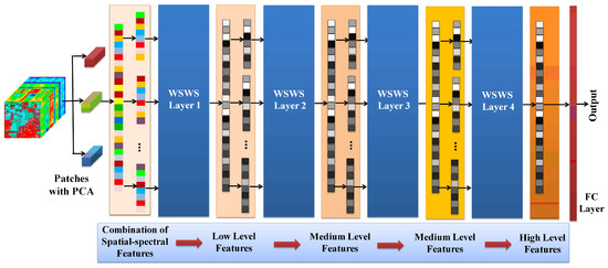
Figure 3. Learning spatial and spectral features using multiple WSWS layers.

3. Datasets and Experimental Settings

3.1. Dataset Description

Three typical hyperspectral remote sensing datasets including Pavia University (PU, Pavia, Italy), the Kennedy Space Center (KSC, Merritt Island, FL, USA), and Salinas hyperspectral images were used to test the performance of the WSWS Net. The datasets are as in Table 2, and described in detail below

Table 2. Description of hyperspectral remote sensing datasets.

NO.	Pavia University		KSC		Salinas
	Class Name	NO.	Class Name	NO.	Class Name	NO.
1	Asphalt	6631	Scrub	347	Brocoli-green-weeds-1	2009
2	Meadows	18,649	Willow swamp	243	Brocoli-green-weeds-2	3726
3	Gravel	2099	CP hammock	256	Fallow	1976
4	Trees	3064	Slash pine	252	Fallow-rough-plow	1394
5	Painted metal sheets	1345	Oak/broadleaf	161	Fallow-smooth	2678
6	Bare soil	5029	Hardwood	229	Stubble	3959
7	Bitumen	1330	Swamp	105	Celery	3579
8	Self-blocking bricks	3682	Graminoid marsh	390	Grapes-untrained	11,271
9	Shadows	947	Spartina marsh	520	Soil-vinyard-develop	6203
10			Cattail marsh	404	Corn-senesced-green-weeds	3278
11			Salt marsh	419	Lettuce-romaine-4wk	1068
12			Mud flats	503	Lettuce-romaine-5wk	1927
13			Water	927	Lettuce-romaine-6wk	916
14					Lettuce-romaine-7wk	1070
15					Vinyard-untrained	7268
16					Vinyard-vertica-trellis	1807
Total		42,776		5211		54,129

(1) Pavia University: The Pavia University scenes were acquired by the ROSIS sensor over Pavia. It has a dimension of $610\times 610$ (after discarding the pixels without information, the dimension is $610\times 340$). There are 9 classes in the image ground truth.

(2) KSC: The KSC dataset was acquired over the Kennedy Space Center in Florida. It has 176 bands after removing water absorption and low SNR bands from 224 bands. The image size of each band is $512\times 614$, and there are 13 classes for classification.

(3) Salinas: It was gathered in Salinas valley, California, including 204 bands after abandoning bands of water absorption. Its dimension is $512\times 217$ pixels, and the class number is 16.

3.2. Experimental Setup

The experiments were implemented using a Dell Work Station with Intel-i7-8700K CPU @ 3.7GHz, 32G memory. Principal component analysis (PCA) was used to reduce the number of redundant spectral bands to 15. For the proposed WSWS Net, the patch size of $9\times 9$ was used for Pavia Universiy, $11\times 11$ for KSC, and $13\times 13$ for Salinas datasets, which were determined in the section of discussions. The pixel at the center of the patches was taken as an independent instance for training, validation, and testing. The proportions of instances for training and validation were 0.2, and the remaining instances were reserved for the testing process. The overall accuracy (OA), average accuracy (AA), and Kappa coefficient were used to evaluate the performance. OA and AA are defined as

$$OA=\frac{N_{correct}}{N_{total}}$$

(17)

$$AA=\frac{1}{C}\sum _{i=1}^C\frac{N_{correct\_i}}{N_{total\_i}}$$

(18)

where $N_{correct}$ and $N_{total}$ are the correctly classified and the total number of testing samples, respectively. $N_{correct\_i}$ and $N_{total\_i}$ are the numbers of correctly classified and testing samples for class i, respectively.

The proposed WSWS Net can learn spatial and spectral features hierarchically by multiple WSWS layers. The key hyperparameters, including the sliding window size, numbers of transform kernels, and subsampling in each WSWS layer, are fine-tuned (increased) from the first layer to succeeding layers. The initial settings of each WSWS layer are the same. The initial sliding window size was 0.9 of the length of the input vectors, and the initial numbers of transform kernels and subsampling were 6 and 3, respectively. Then, the validation set was used to find the proper parameters. The number of training samples and the size of patches are also important for the classification performance of hyperspectral remote sensing images, as discussed in Section 4.

The proposed method was compared with other methods including multilayer perceptron (MLP), stacked autoencoder (SAE), radial basis function (RBF), CNN, RBF ensemble, and CNN ensemble. The hyperparameters of these models were fine-tuned using the validation set.

4. Experimental Results

4.1. Classification Results for Pavia University

In this experiment, the proposed WSWS Net included four WSWS layers. The window sizes, numbers of transform kernels, and subsampling layer were 13, 40, and 20 for the first WSWS layer, respectively; 0.8 of the length of input vector, 16, and 8 for the second WSWS layer, respectively; 0.9 of the length of input vector, 6, and 3 for the third WSWS layer, respectively; and 0.9 of the length of input vector, 6, and 3 for the fourth WSWS layer, respectively. The compared method MLP had 1000 hidden units. The RBF had 2000 Gaussian kernels with the centers of the Gaussian kernels randomly chosen from the training samples. The SAE had 400 hidden units for encoder, and 50 hidden units for decoder. The architecture of the CNN included 6 convolutional kernels, a pooling layer with scale 2, 12 convolutional kernels, and a pooling layer with scale 2. The RBF ensemble included 5 RBF networks with the same architecture as the compared single RBF network. The CNN ensemble included 5 CNNs with the same architecture as the compared single CNN. Different sizes of input patches were selected for different methods to obtain the best performance and fair comparisons. The size of input patches was $9\times 9$ for MLP and SAE, $5\times 5$ for RBF and RBF ensemble, and $3\times 3$ for CNN and CNN ensemble.

The experimental results are shown in Table 3 and Figure 4. It is observed from the table that the proposed method had the best test performance including OA, AA, and Kappa coefficient, which were 99.19%, 98.51%, and 98.93%, respectively. It is seen that more balanced classification results were achieved in each class for the proposed WSWS Net. The MLP, RBF, and CNN have good performances, which are higher than 93% compared with SAE. The ensemble methods of RBFE and CNNE can help improve the classification performances of RBF and CNN. It is observed in Figure 4 that the proposed WSWS Net had a much smoother prediction result in the areas without label information. This can be seen, for example, in the regions with brown color (bare soil) compared with CNNE and RBFE methods, especially in related images. The testing time was also compared with these methods, and it is seen that the proposed WSWS Net achieved 6.4s, which is faster than RBFE and CNNE. Although MLP, RBF, SAE, and CNN were faster, the classification performances are lower than that of the proposed WSWS Net. The proposed method was also compared with a recently proposed [39] method, which uses spectral blocks to convert the high-dimensional data into small subsets to accelerate the computing resources. It is seen that the WSWS has greater OA and Kappa than SMSB. The testing time of SMSB is 61 s, which is slower than WSWS Net, but the experimental platform is not the same.

Table 3. Classification results of different methods for Pavia University.

Class NO.	Class Name	MLP	RBF	SAE	CNN	RBFE	CNNE	SMSB [39]	WSWS
1	Asphalt	97.13	97.65	97.43	96.18	98.99	95.22	99.11	99.10
2	Meadows	98.43	99.53	98.60	96.69	99.86	99.03	98.97	100.00
3	Gravel	85.15	80.62	0.00	80.86	81.43	82.92	98.89	93.01
4	Trees	95.05	93.84	91.35	87.21	95.43	87.00	98.74	98.37
5	Painted metal sheets	99.88	91.58	99.75	99.63	99.88	99.75	100	99.88
6	Bare soil	96.35	87.06	76.30	88.30	81.67	80.88	99.87	99.97
7	Bitumen	90.85	90.30	0.00	82.58	84.46	90.73	99.79	99.00
8	Self-blocking bricks	93.21	92.43	85.84	94.12	92.85	93.44	98.99	98.33
9	Shadows	99.30	94.84	95.61	99.30	97.72	99.47	98.04	98.95
OA (%)		96.47	95.18	86.23	93.66	95.23	93.95	99.11	99.19
AA (%)		95.04	91.98	71.64	91.65	92.41	92.05	99.16	98.51
Kappa (%)		95.36	93.66	82.03	91.72	93.72	92.05	98.79	98.93
Test Time (s)		1.3	1.5	0.2	3.7	8.6	22.2	61.0	6.4

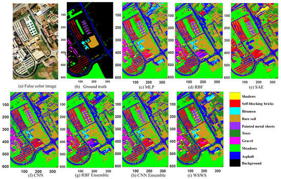
Figure 4. Classification results of Pavia University data. (a) Original image, (b) ground truth (there are no class labels for the black background), (c) multilayer perceptron (MLP), (d) radial basis function (RBF), (e) stacked autoencoder (SAE), (f) convolutional neural network (CNN), (g) RBE ensemble, (h) CNN ensemble, and (i) WSWS.

4.2. Classification Results for KSC

In this experiment, the WSWS Net included four WSWS layers, and the window sizes, numbers of transform kernels, and subsampling layer were 77, 10, and 5 for the first WSWS layer, respectively; 0.9 of the length of input vector, 10, and 5 for the second WSWS layer; 0.9 of the length of input vector, 8, 4 for the third WSWS layer; and 0.9 of the length of input vector, 6, and 3 for the fourth WSWS layer, respectively. The compared method MLP had 1000 hidden units. The RBF had 1000 Gaussian kernels, and the centers of the Gaussian kernels were randomly chosen from the training samples. The SAE had 300 hidden units for encoder, and 50 hidden units for decoder, respectively. The architectures of the CNN and CNN ensemble were the same as for Pavia University. The RBF ensemble included 5 RBF networks with the same architecture as the compared single RBF network. Different sizes of input patches were selected for different methods to present the best performance and fair comparisons. The size of input patches for MLP, SAE, RBF, RBF ensemble, CNN, and CNN ensemble was the same as for Pavia University.

It is observed from Table 4 that the WSWS had the best OA, AA, and Kappa coefficient with the test set, which were 99.87%, 99.71%, and 99.86%, respectively. Eight of 13 performances of single classes reached the accuracy 100%. The performances for each class had more balanced accuracy than other compared methods. The typical result was that, although MLP had OA, AA, and Kappa coefficient as high as 97.95%, 96.60%, and 97.72%, respectively, the lowest accuracy of class no.4 was only 79.61, compared to the highest accuracies of class no. 7, 8, 9, and 13, which were 100%. MLP, RBF, and CNN can achieve test OAs higher than 95%. The ensemble methods of RBFE and CNNE have higher test performances than those of RBF and CNN, respectively. Other than classes no. 3 and no. 5, the proposed WSWS Net has the best test performance on other single classes. It is seen from Figure 5 that the proposed WSWS Net had a much smoother prediction result compared with other methods. For example, this can be seen in the regions with yellow color representing hardwood compared with MLP, CNN, and CNNE methods in related images. It is also seen in the regions with pink color (slash pine) compared with RBF, and RBFE methods in corresponding images. The testing time was also shown in the table, and it is observed that the WSWS Net consumes 1.9 s, which is faster than RBFE and CNNE. Although other methods were faster, the classification performances are not as good as the WSWS Net.

Table 4. Classification results of different methods for KSC.

Class NO.	Class Name	MLP	RBF	SAE	CNN	RBFE	CNNE	WSWS
1	Scrub	99.78	98.47	98.69	97.37	96.94	97.81	100.00
2	Willow swamp	99.31	88.28	71.03	94.48	92.41	94.48	100.00
3	CP hammock	92.86	96.75	93.51	95.45	96.10	98.70	99.35
4	Slash pine	79.61	64.47	34.21	76.97	71.71	70.39	100.00
5	Oak/broadleaf	87.63	90.72	0.00	72.16	92.78	69.07	96.91
6	Hardwood	99.27	88.32	2.19	83.21	83.21	86.13	100.00
7	Swamp	100.00	96.83	12.70	100.00	95.24	90.48	100.00
8	Graminoid marsh	100.00	98.07	83.01	96.53	94.98	99.61	100.00
9	Spartina marsh	100.00	100.00	99.36	100.00	100.00	100.00	100.00
10	Cattail marsh	99.59	99.59	100.00	100.00	97.93	100.00	100.00
11	Salt marsh	98.41	90.84	97.61	100.00	95.62	100.00	100.00
12	Mud flats	99.34	98.01	92.68	96.01	98.67	98.34	100.00
13	Water	100.00	100.00	100.00	100.00	100.00	100.00	100.00
OA (%)		97.95	95.36	83.72	95.75	95.52	95.97	99.87
AA (%)		96.60	93.10	68.31	93.25	93.51	92.69	99.71
Kappa (%)		97.72	94.85	82.03	95.28	95.03	95.52	99.86
Test Time (s)		0.6	0.1	0.1	0.9	2.2	5.9	1.9

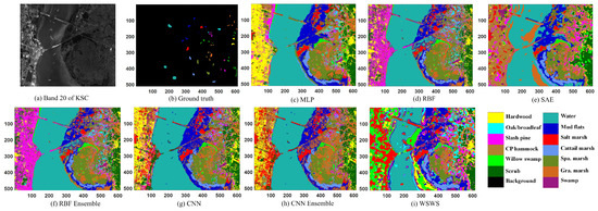
Figure 5. Classification results of KSC data. (a) Original image, (b) ground truth (there are no class labels for the black background), (c) MLP, (d) RBF, (e) SAE, (f) CNN, (g) RBE ensemble, (h) CNN ensemble, and (i) WSWS.

4.3. Classification Results for Salinas

The proposed WSWS Net included four WSWS layers in this experiment. The window sizes, numbers of transform kernels, and subsampling layer were 33, 20, and 10 for the first WSWS layer; 0.9 of the length of input vector, 20, and 10 for the second and third WSWS layers; 0.9 of the length of input vector, 6, and 3 for the third WSWS layer; and 0.7 of the length of input vector, 20, and 10 for the fourth WSWS layer, respectively. The compared method MLP included 2000 hidden units. The RBF had 2000 Gaussian kernels, and the centers of the Gaussian kernels were randomly chosen from the training samples. The SAE had 200 hidden units for encoder, and 50 hidden units for decoder. The architecture of the CNN and CNN ensemble were the same as for Pavia University and KSC. The RBF ensemble was composed of five RBF networks with the same architecture as the compared single RBF network. The size of input patches was $9\times 9$ for MLP and SAE, $5\times 5$ for RBF and RBF ensemble, and $3\times 3$ for CNN and CNN ensemble, respectively.

The experimental results are shown in Table 5 and Figure 6. It is observed that the proposed method had the best classification results in terms of OA, AA, and Kappa coefficient (99.67%, 99.63%, and 99.63%, respectively). The performances for single classes had the most balanced accuracy among all the methods, which were in the range from 97.73% to 100.00%. The RBF, SAE, and CNN have test OAs higher than 92%. The test performances of the RBFE and CNNE are higher than those of RBF and CNN, respectively. The testing time was given with these methods in the table, and it is seen that the proposed WSWS Net achieved 11.8 s, and it is faster than RBFE and CNNE. Although MLP, RBF, SAE, and CNN were faster, the classification performance of the WSWS Net is much better than these methods. The proposed method was also compared with the SMSB method, and it is seen that the WSWS has better performance than SMSB. The testing time of SMSB is slower than WSWS Net, but the experimental platform is not the same.

Table 5. Classification results of different methods for Salinas.

Class NO.	Class Name	MLP	RBF	SAE	CNN	RBFE	CNNE	SMSB [39]	WSWS
1	Bro.-gw-1	100.00	99.75	99.17	98.51	100.00	98.92	99.78	100.00
2	Bro.-gw-2	100.00	100.00	99.87	99.82	100.00	99.87	99.97	99.87
3	Fallow	99.41	99.83	92.16	99.66	99.75	99.41	99.94	98.82
4	Fal.-rough-plow	99.52	99.52	97.61	98.68	99.52	98.80	99.28	97.73
5	Fallow-smooth	97.70	97.14	98.63	99.38	97.14	99.75	99.54	99.38
6	Stubble	100.00	100.00	99.92	99.96	100.00	99.92	99.97	99.96
7	Celery	0.00	100.00	99.63	99.95	100.00	99.95	99.88	99.91
8	Gra.-untrained	90.64	91.22	89.75	74.24	91.62	90.17	98.87	99.72
9	Soil-vd	100.00	100.00	99.87	100.00	100.00	100.00	99.91	99.76
10	Corn-sgw	99.08	98.98	96.19	93.44	99.08	93.13	98.85	99.64
11	Let.-r-4wk	99.53	99.69	93.75	96.72	99.69	97.19	99.79	100.00
12	Let.-r-5wk	100.00	100.00	98.96	99.74	100.00	99.91	99.94	99.91
13	Let.-r-6wk	99.64	99.27	100.00	98.91	99.64	99.82	99.03	99.82
14	Let.-r-7wk	99.84	99.69	96.42	100.00	99.53	99.69	98.86	100.00
15	Vinyard-u	85.53	79.33	77.50	88.65	79.54	75.16	97.63	99.52
16	Vinyard-v-t	99.91	100.00	99.45	98.53	99.91	98.62	99.92	100.00
OA (%)		89.27	95.14	93.86	92.42	95.26	93.97	99.26	99.67
AA (%)		91.92	97.78	96.18	96.64	97.84	96.90	99.45	99.63
Kappa (%)		88.20	94.64	93.23	91.69	94.77	93.35	99.17	99.63
Test Time (s)		4.1	4.6	0.7	4.5	25.5	46.9	51.0	11.8

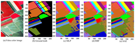
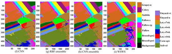
Figure 6. Classification results of Salinas data. (a) Original image, (b) ground truth (there are no class labels for the black background), (c) MLP, (d) RBF, (e) SAE, (f) CNN, (g) RBE ensemble, (h) CNN ensemble, and (i) WSWS.

5. Discussion

5.1. The Effects of Different Ratio of Training Samples

As more training samples of hyperspectral remote sensing images are provided, the test accuracy can be improved, and it will finally stop increasing or increase slowly [29,40]. Therefore, there is a trade-off between the ratio of training samples and the test performance of hyperspectral remote sensing images. That may be because a given number of training samples with given sizes of patches provides limited spatial and spectral information for the learning models. Different ratios of training samples were used to test the influence to the performance of the proposed WSWS Net. The patch sizes here of the WSWS Net are $7\times 7$ for Pavia University data, and $9\times 9$ for KSC and Salinas datasets. Other settings are the same as the experiment in Section 4.

The results are shown in Table 6 and Figure 7. It is observed from the table that as the training samples increased, the test performances were also increased. For Pavia University, the test performance increased until the train ratio reached 0.2, then it decreased and fluctuated. For KSC data, the test performance increased until the training ratio reached 0.3. This is mainly because this dataset is rather small; therefore, the WSWS Net can learn the data more easily without overfitting. For Salinas data, the trend is similar to that of the Pavia University, and the test performance dropped when the ratio was higher than 0.25.

Table 6. Test accuracies of different partition of training Samples on Pavia Center, Pavia University, and KSC datasets.

Ratio of Training Samples	Pavia Univ./(%)			KSC/(%)			Salinas (%)
	OA	AA	Kappa	OA	AA	Kappa	OA	AA	Kappa
0.05	96.33	94.21	95.16	91.94	88.23	91.08	97.19	98.20	96.89
0.1	98.38	97.34	97.86	96.38	94.24	95.98	98.62	98.97	98.47
0.15	98.84	98.07	98.46	99.21	98.39	99.12	99.19	99.23	99.10
0.2	99.11	98.44	98.82	99.52	99.24	99.47	99.44	99.57	99.38
0.25	98.92	97.94	98.56	99.65	99.37	99.62	99.48	99.64	99.42
0.3	98.96	98.17	98.62	99.79	99.57	99.77	99.37	99.47	99.30

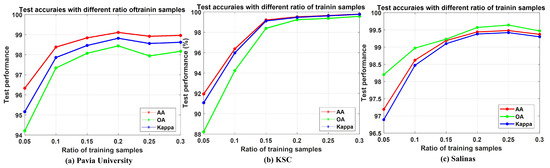
Figure 7. Test performance with different ratio of training samples on different hyperspectral datasets. (a) Pavia University. (b) KSC. (c) Salinas.

5.2. The Effects of Different Neighborhood Sizes

The different neighborhood sizes or patch sizes of the hyperspectral remote sensing images have an important influence on the classification performance of learning models [11,30]. Therefore, it is also discussed here for the proposed WSWS Net. The number of spectral bands after PCA was still reduced to 15. The WSWS Net settings are the same as the experiment in Section 4.

The results are shown in Table 7. As the size of path size increased, the performance was improved. It is observed from the table that neither too small nor too big patch size is best for Pavia University and KSC hyperspectral image classification. For Pavia University and KSC datasets, the best test performance was obtained with the patch size $9\times 9$ and $11\times 11$, respectively. Then, the performances decreased. For Salinas data, the test performance continued increasing until the patch size reached $13\times 13$. The AA grew with a little fluctuation as the size of patches increased for Salinas dataset.

Table 7. Test accuracies with different neighborhood sizes of Pavia Center, Pavia University, and KSC datasets.

Neighborhood Sizes	Pavia Univ./(%)			KSC/(%)			Salinas/ (%)
	OA	AA	Kappa	OA	AA	Kappa	OA	AA	Kappa
$3\times 3$	95.13	92.41	93.61	80.46	69.71	78.53	92.83	96.66	92.12
$5\times 5$	98.22	96.87	97.65	95.87	93.14	95.42	93.07	96.55	92.37
$7\times 7$	99.11	98.44	98.82	98.31	97.00	98.11	98.67	99.15	98.52
$9\times 9$	99.19	98.51	98.93	99.52	99.24	99.47	99.44	99.57	99.38
$11\times 11$	99.17	98.63	98.91	99.87	99.71	99.86	99.56	99.53	99.51
$13\times 13$	97.45	96.36	96.64	99.26	99.12	99.18	99.67	99.63	99.63

5.3. Visualization of Different Layers of Extracted features

The extracted features from WSWS layers are visualized in this section. These features from the first and fourth layers are obtained with two steps: (1) The subsampled output vectors of the WSWS layers are reorganized for the related input elements. (2) These reorganized data are summed together, and the vector of corresponding input vector is generated, which can be seen as the extracted features from the current WSWS layer.

For Pavia University and Salinas data, the extracted features from the above two layers of 30 training samples were stacked together, and for KSC data, these features of all training samples were stacked because this dataset is smaller. The visualization results are shown in Figure 8, Figure 9 and Figure 10. Four classes are chosen and shown. For each class itself, it is seen the stacked features in the first and fourth layers are very similar for the corresponding layer, and for different classes, it is seen that the extracted features are very different. This demonstrates that the WSWS layers can extract features effectively, and how the proposed WSWS Net can classify hyperspectral images effectively.

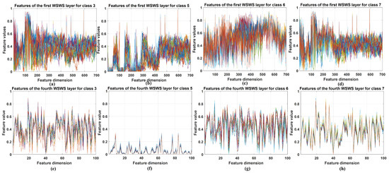
Figure 8. Visualization of the selected extracted features from the first and fourth WSWS layers of the Pavia University dataset. (a–d) The stacked results of extracted features of class 3, 5, 6, and 7 in the first WSWS layers from 30 training samples. (e–h) The stacked results of extracted features of class 3, 5, 6, and 7 in the fourth WSWS layers from 30 training samples.

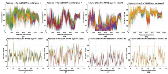
Figure 9. Visualization of the selected extracted features from the first and fourth WSWS layers of the KSC dataset. (a–d) The stacked results of extracted features of class 1, 7, 10, and 13 in the first WSWS layers from all the training samples. (e–h) The stacked results of extracted features of class 1, 7, 10, and 13 in the fourth WSWS layers from all the training samples.

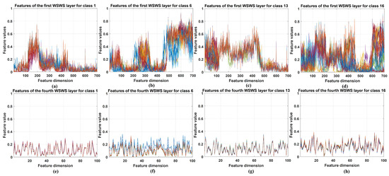
Figure 10. Visualization of the selected extracted features from the first and fourth WSWS layers of the Salinas dataset. (a–d) The stacked results of extracted features of class 1, 6, 13, and 16 in the first WSWS layers from 30 training samples. (e–h) The stacked results of extracted features of class 1, 6, 13, and 16 in the fourth WSWS layers from 30 training samples.

6. Conclusions

Hyperspectral remote sensing images provide abundant information both in spatial and spectral domains. It is usually very expensive to acquire a large number of hyperspectral images, and it is hard to use them effectively for land cover classification with such a large number of bands. CNN-based methods have been extended to HSI classification and achieved excellent performance. The limited training samples of HSI with small patches makes it difficult to utilize the advantages of deep learning models, and the deep learning models with a large number of weights usually need a long training time. We propose a WSWS Net for HSI classification, which is composed of layers of transform kernels with sliding windows and subsampling (WSWS). First, it is extended in the wide direction to learn both the spatial and spectral features sufficiently using transform kernels and wide sliding windows. The parameters of these kernels can be learned easily by unsupervised method or choosing them randomly from training samples. Then, the learned features are subsampled to reduce computational loads and avoid overfitting. Second, the layers of WSWS are organized in a cascade to learn higher level spatial and spectral features efficiently. Finally, the proposed WSWS Net is trained fast by only learning linear weights with least squares method.

The proposed method was tested with Pavia University, KSC, and Salinas hyperspectral remote sensing datasets. It is seen from the experimental results that the proposed WSWS Net achieves excellent performance compared with both shallow and deep learning methods. The influence of neighborhood size and ratio of training samples on the test performance was also discussed, and it is observed that neighborhood sizes such as $9\times 9$ and a ratio of 0.2 for training samples can give good enough performance for WSWS Net. The extracted features of different WSWS layers were also visualized to show that the WSWS Net can extract different features in different classes for classification effectively. In future work, the scalability of the proposed method will be explored mainly with the iterative method or ensemble method to learn hyperspectral images with a large number of pixels efficiently. One of the important problems is to deal with hyperspectral images containing a large number of mixed pixels by extracting endmembers and abundances in these pixels. We will also combine the hyperspectral unmixing methods together with the proposed classification method to evaluate classification performance more precisely in future work.

References

- Li, W.; Wu, G.; Zhang, F.; Du, Q. Hyperspectral image classification using deep pixel-pair features. IEEE Trans. Geosci. Remote Sens. 2016, 55, 844–853. [Google Scholar] [CrossRef]
- Tarabalka, Y.; Fauvel, M.; Chanussot, J.; Benediktsson, J.A. SVM-and MRF-based method for accurate classification of hyperspectral images. IEEE Geosci. Remote Sens. Lett. 2010, 7, 736–740. [Google Scholar] [CrossRef]
- Xi, J.; Ersoy, O.K.; Fang, J.; Wu, T.; Wei, X.; Zhao, C. Parallel Multistage Wide Neural Network; Department of Electrical and Computer Engineering Technical Reports; Purdue University: West Lafayette, Indiana, 2020; Volume 757. [Google Scholar]
- Li, J.; Bioucas-Dias, J.M.; Plaza, A. Semisupervised hyperspectral image classification using soft sparse multinomial logistic regression. IEEE Geosci. Remote Sens. Lett. 2012, 10, 318–322. [Google Scholar]
- Fauvel, M.; Benediktsson, J.A.; Chanussot, J.; Sveinsson, J.R. Spectral and spatial classification of hyperspectral data using SVMs and morphological profiles. IEEE Trans. Geosci. Remote Sens. 2008, 46, 3804–3814. [Google Scholar] [CrossRef]
- Li, J.; Bioucas-Dias, J.M.; Plaza, A. Spectral–spatial hyperspectral image segmentation using subspace multinomial logistic regression and Markov random fields. IEEE Trans. Geosci. Remote Sens. 2011, 50, 809–823. [Google Scholar] [CrossRef]
- Chen, Y.; Nasrabadi, N.M.; Tran, T.D. Hyperspectral image classification using dictionary-based sparse representation. IEEE Trans. Geosci. Remote Sens. 2011, 49, 3973–3985. [Google Scholar] [CrossRef]
- Li, J.; Marpu, P.R.; Plaza, A.; Bioucas-Dias, J.M.; Benediktsson, J.A. Generalized composite kernel framework for hyperspectral image classification. IEEE Trans. Geosci. Remote Sens. 2013, 51, 4816–4829. [Google Scholar] [CrossRef]
- Lee, H.; Kwon, H. Going deeper with contextual CNN for hyperspectral image classification. IEEE Trans. Image Process. 2017, 26, 4843–4855. [Google Scholar] [CrossRef]
- Mei, S.; Ji, J.; Hou, J.; Li, X.; Du, Q. Learning sensor-specific spatial-spectral features of hyperspectral images via convolutional neural networks. IEEE Trans. Geosci. Remote Sens. 2017, 55, 4520–4533. [Google Scholar] [CrossRef]
- Gao, Q.; Lim, S.; Jia, X. Hyperspectral image classification using convolutional neural networks and multiple feature learning. Remote Sens. 2018, 10, 299. [Google Scholar] [CrossRef]
- Wang, W.; Dou, S.; Jiang, Z.; Sun, L. A fast dense spectral–spatial convolution network framework for hyperspectral images classification. Remote Sens. 2018, 10, 1068. [Google Scholar] [CrossRef]
- Paoletti, M.; Haut, J.; Plaza, J.; Plaza, A. A new deep convolutional neural network for fast hyperspectral image classification. ISPRS J. Photogramm. Remote Sens. 2018, 145, 120–147. [Google Scholar] [CrossRef]
- Zhang, M.; Li, W.; Du, Q. Diverse region-based CNN for hyperspectral image classification. IEEE Trans. Image Process. 2018, 27, 2623–2634. [Google Scholar] [CrossRef] [PubMed]
- Cheng, G.; Li, Z.; Han, J.; Yao, X.; Guo, L. Exploring hierarchical convolutional features for hyperspectral image classification. IEEE Trans. Geosci. Remote Sens. 2018, 56, 6712–6722. [Google Scholar] [CrossRef]
- Zhang, L.; Zhang, L.; Du, B. Deep learning for remote sensing data: A technical tutorial on the state of the art. IEEE Geosci. Remote Sens. Mag. 2016, 4, 22–40. [Google Scholar] [CrossRef]
- Mou, L.; Ghamisi, P.; Zhu, X.X. Deep recurrent neural networks for hyperspectral image classification. IEEE Trans. Geosci. Remote Sens. 2017, 55, 3639–3655. [Google Scholar] [CrossRef]
- Mei, X.; Pan, E.; Ma, Y.; Dai, X.; Huang, J.; Fan, F.; Du, Q.; Zheng, H.; Ma, J. Spectral-spatial attention networks for hyperspectral image classification. Remote Sens. 2019, 11, 963. [Google Scholar] [CrossRef]
- Roy, S.K.; Krishna, G.; Dubey, S.R.; Chaudhuri, B.B. HybridSN: Exploring 3-D–2-D CNN feature hierarchy for hyperspectral image classification. IEEE Geosci. Remote Sens. Lett. 2019, 17, 277–281. [Google Scholar] [CrossRef]
- Zheng, J.; Feng, Y.; Bai, C.; Zhang, J. Hyperspectral Image Classification Using Mixed Convolutions and Covariance Pooling. IEEE Trans. Geosci. Remote Sens. 2020, 59, 522–534. [Google Scholar] [CrossRef]
- Gong, Z.; Zhong, P.; Yu, Y.; Hu, W.; Li, S. A CNN With Multiscale Convolution and Diversified Metric for Hyperspectral Image Classification. IEEE Trans. Geosci. Remote Sens. 2019, 57, 3599–3618. [Google Scholar] [CrossRef]
- Haut, J.M.; Paoletti, M.E.; Plaza, J.; Li, J.; Plaza, A. Active Learning With Convolutional Neural Networks for Hyperspectral Image Classification Using a New Bayesian Approach. IEEE Trans. Geosci. Remote Sens. 2018, 56, 6440–6461. [Google Scholar] [CrossRef]
- Cao, X.; Yao, J.; Xu, Z.; Meng, D. Hyperspectral image classification with convolutional neural network and active learning. IEEE Trans. Geosci. Remote Sens. 2020. [Google Scholar] [CrossRef]
- Feng, J.; Wu, X.; Shang, R.; Sui, C.; Li, J.; Jiao, L.; Zhang, X. Attention Multibranch Convolutional Neural Network for Hyperspectral Image Classification Based on Adaptive Region Search. IEEE Trans. Geosci. Remote Sens. 2020. [Google Scholar] [CrossRef]
- Chen, Y.; Zhu, K.; Zhu, L.; He, X.; Ghamisi, P.; Benediktsson, J.A. Automatic Design of Convolutional Neural Network for Hyperspectral Image Classification. IEEE Trans. Geosci. Remote Sens. 2019, 57, 7048–7066. [Google Scholar] [CrossRef]
- Hong, D.; Wu, X.; Ghamisi, P.; Chanussot, J.; Yokoya, N.; Zhu, X.X. Invariant attribute profiles: A spatial-frequency joint feature extractor for hyperspectral image classification. IEEE Trans. Geosci. Remote Sens. 2020, 58, 3791–3808. [Google Scholar] [CrossRef]
- Wang, J.; Gao, F.; Dong, J.; Du, Q. Adaptive DropBlock-Enhanced Generative Adversarial Networks for Hyperspectral Image Classification. IEEE Trans. Geosci. Remote Sens. 2020. [Google Scholar] [CrossRef]
- Shen, Y.; Zhu, S.; Chen, C.; Du, Q.; Xiao, L.; Chen, J.; Pan, D. Efficient Deep Learning of Nonlocal Features for Hyperspectral Image Classification. IEEE Trans. Geosci. Remote Sens. 2020. [Google Scholar] [CrossRef]
- Liu, Q.; Xiao, L.; Yang, J.; Chan, J.C.W. Content-Guided Convolutional Neural Network for Hyperspectral Image Classification. IEEE Trans. Geosci. Remote Sens. 2020, 58, 6124–6137. [Google Scholar] [CrossRef]
- Tang, X.; Meng, F.; Zhang, X.; Cheung, Y.; Ma, J.; Liu, F.; Jiao, L. Hyperspectral Image Classification Based on 3-D Octave Convolution With Spatial-Spectral Attention Network. IEEE Trans. Geosci. Remote Sens. 2020. [Google Scholar] [CrossRef]
- Masarczyk, W.; Głomb, P.; Grabowski, B.; Ostaszewski, M. Effective Training of Deep Convolutional Neural Networks for Hyperspectral Image Classification through Artificial Labeling. Remote Sens. 2020, 12, 2653. [Google Scholar] [CrossRef]
- Okwuashi, O.; Ndehedehe, C.E. Deep support vector machine for hyperspectral image classification. Pattern Recognit. 2020, 103, 107298. [Google Scholar] [CrossRef]
- Cao, F.; Guo, W. Cascaded dual-scale crossover network for hyperspectral image classification. Knowl. Based Syst. 2020, 189, 105122. [Google Scholar] [CrossRef]
- Neyshabur, B.; Li, Z.; Bhojanapalli, S.; LeCun, Y.; Srebro, N. The role of over-parametrization in generalization of neural networks. In Proceedings of the International Conference on Learning Representations, Vancouver, BC, Canada, 30 April–3 May 2019. [Google Scholar]
- Lee, J.; Xiao, L.; Schoenholz, S.S.; Bahri, Y.; Sohl-Dickstein, J.; Pennington, J. Wide neural networks of any depth evolve as linear models under gradient descent. arXiv 2019, arXiv:1902.06720. [Google Scholar]
- Cheng, H.T.; Koc, L.; Harmsen, J.; Shaked, T.; Chandra, T.; Aradhye, H.; Anderson, G.; Corrado, G.; Chai, W.; Ispir, M.; et al. Wide & deep learning for recommender systems. In Proceedings of the 1st Workshop on Deep Learning for Recommender Systems, Boston, MA, USA, 15 September 2016; pp. 7–10. [Google Scholar]
- Worrall, D.E.; Garbin, S.J.; Turmukhambetov, D.; Brostow, G.J. Harmonic networks: Deep translation and rotation equivariance. In Proceedings of the IEEE Conference on Computer Vision and Pattern Recognition, Honolulu, HI, USA, 21–26 July 2017; pp. 5028–5037. [Google Scholar]
- Liu, C.; Li, J.; He, L.; Plaza, A.; Li, S.; Li, B. Naive Gabor Networks for Hyperspectral Image Classification. IEEE Trans. Neural Networks Learn. Syst. 2020. [Google Scholar] [CrossRef] [PubMed]
- Azar, S.G.; Meshgini, S.; Rezaii, T.Y.; Beheshti, S. Hyperspectral image classification based on sparse modeling of spectral blocks. Neurocomputing 2020, 407, 12–23. [Google Scholar] [CrossRef]
- Yu, S.; Jia, S.; Xu, C. Convolutional neural networks for hyperspectral image classification. Neurocomputing 2017, 219, 88–98. [Google Scholar] [CrossRef]
Publisher’s Note: MDPI stays neutral with regard to jurisdictional claims in published maps and institutional affiliations. |
© 2021 by the authors. Licensee MDPI, Basel, Switzerland. This article is an open access article distributed under the terms and conditions of the Creative Commons Attribution (CC BY) license (http://creativecommons.org/licenses/by/4.0/).