Abstract
Deep learning provides a promising approach for air pollution prediction. The existing deep learning-based predicted models generally consider either the temporal correlations of air quality monitoring stations or the nonlinear relationship between the PM2.5 (particulate matter with an aerodynamic diameter of less than 2.5 μm) concentrations and explanatory variables. Spatial correlation has not been effectively incorporated into prediction models, therefore exhibiting poor performance in PM2.5 prediction tasks. Additionally, determining the manner by which to expand longer-term prediction tasks is still challenging. In this paper, to allow for spatiotemporal correlations, a spatiotemporal convolutional recursive long short-term memory (CR-LSTM) neural network model is proposed for predicting the PM2.5 concentrations in long-term prediction tasks by combining a convolutional long short-term memory (ConvLSTM) neural network and a recursive strategy. Herein, the ConvLSTM network was used to capture the complex spatiotemporal correlations and to predict the future PM2.5 concentrations; the recursive strategy was used for expanding the long-term prediction tasks. The CR-LSTM model was used to realize the prediction of the future 24 h of PM2.5 concentrations for 12 air quality monitoring stations in Beijing by configuring both the appropriate time lag derived from the temporal correlations and the spatial neighborhood, including the hourly historical PM2.5 concentrations, the daily mean meteorological data, and the annual nighttime light and normalized difference vegetation index (NDVI). The results showed that the proposed CR-LSTM model achieved better performance (coefficient of determination (R2) = 0.74; root mean square error (RMSE) = 18.96 μg/m3) than other common models, such as multiple linear regression (MLR), support vector regression (SVR), the conventional LSTM model, the LSTM extended (LSTME) model, and the temporal sliding LSTM extended (TS-LSTME) model. The proposed CR-LSTM model, implementing a combination of geographical rules, recursive strategy, and deep learning, shows improved performance in longer-term prediction tasks.
1. Introduction
Fine particulate matter with an aerodynamic diameter <2.5 μg (PM2.5) is one of the most significant sources of air pollution in urban areas [1,2]. Long-term exposure to heavy PM2.5 concentrations is related to adverse effects on human organs and, furthermore, causes cardiovascular diseases [3,4,5,6,7]. Many cities in China still face haze pollution due to the energy consumption caused by human activities and economic development in recent years [8]. PM2.5 pollution has received increasing attention from the public in China since 2013 [9]. Since 2013, approximately 1500 air quality monitoring stations across China have been built to accurately monitor the ground-level air quality conditions in real time. Therefore, it is meaningful to predict PM2.5 concentrations in advance using these established air quality monitoring stations to prevent major accidents caused by air pollution, thus assisting in atmospheric management decisions and controlling major air pollution events.
Previous studies [3,10,11] introduced two classes of models for predicting PM2.5 concentrations—deterministic models and statistical models. Deterministic models predict PM2.5 concentrations by simulating physical transmission and the chemical reactions of air pollutants [3,12]. Despite the progress made by those methods, they suffer from expensive computation due to the photochemical dispersion mechanism and uncertainties in emissions, which is not suitable for air quality prediction in large-scale areas [11,13,14,15]. Statistical models, mainly referring to machine- or deep-learning techniques, can fit the complicated relationship between PM2.5 concentrations and exogenous variables [16,17] and reach a prediction accuracy almost comparable to deterministic models [18,19]. Due to their incredible speed, lower costs, and lower requirement for prior knowledge, statistical models are widely used in prediction tasks [17,20,21,22,23,24]. With improvements in computational capacity and deep learning theory, these models can achieve better performance in PM2.5 concentrations prediction tasks, providing a promising prospect for expanding the application of statistical models in atmospheric environmental science [16,17,25].
Existing studies show that machine learning- and deep learning-based models have been widely applied in atmospheric environmental modeling for the monitoring and prediction of air pollutants, such as the multilayer perceptron (MLP) model [26,27], the backpropagation neural network (BPNN) model [28], support vector regression (SVR) [28,29], the random forest (RF) model [30,31,32], the general regression neural network (GRNN) model [28,33], the recurrent neural network (RNN) model [34], and long short-term memory (LSTM)-based models [11,35,36,37,38]. The careful reasoning process in machine learning-based models (such as MLP, SVR, and RF) is comparable to mathematical reasoning [11]. However, those models generally exhibit linear relationships between PM2.5 concentrations and exogenous variables. The models’ structures are relatively simple, resulting in disadvantages in extracting the complex nonlinear relationships between input and output variables [3,39]. Additionally, the fault-tolerant ability of machine learning-based models for training samples is unsatisfactory. However, deep learning-based models have satisfactory addictiveness and robustness and can overcome the defects of machine learning-based models [17,22]. Among those deep learning-based prediction models (such as GRNN, BPNN, RNN, and LSTM), the LSTM model can capture temporal autocorrelations and can be widely used in prediction tasks by configuring the corresponding mechanisms for historical time series data [11,20]. More importantly, the LSTM model can overcome gradient explosion and disappearance in error backpropagation and is much better at capturing long short-term information [11,36]. Many LSTM-based models for predicting air quality have been proposed, such as LSTM extended (LSTME) [40], convolutional LSTM extended (C-LSTME) [10], graph convolutional LSTM (GC-LSTM) [24], deep multi-output LSTM (DM-LSTM) [41], Read-first LSTM (RLSTM) [36], convolutional neural network LSTM (CNN-LSTM) [42], and temporal sliding LSTM extended (TS-LSTME) [11] models. However, there are several key limitations in PM2.5 concentration prediction tasks for LSTM-based models. First, various studies have demonstrated that spatiotemporal correlations play a major role in influencing changes in air pollution [3,11,16,22,32,43,44]. Previous studies [11,40] have generally considered the temporal correlations of air pollution. In contrast, spatial correlations have not been effectively incorporated into the corresponding models, affecting these models’ PM2.5 concentration prediction performance. For example, Mao [11] proposed a TS-LSTME model for predicting the 24-h PM2.5 concentration in areas in Jin-jing-ji based on the conventional LSTM model and sliding prediction. Simultaneously, spatial correlations among air quality monitoring stations have only been applied to reference partitioning modeling strategies rather than incorporated into sliding prediction tasks. Therefore, it is worth discussing the manner in which to effectively capture and quantify spatial correlation. Second, conventional LSTM-based models are suitable for long short-term prediction tasks but longer-term prediction tasks (up to or greater than 24-h prediction) generally exhibit poor performance. For example, Wen [10] proposed a C-LSTME model for predicting the PM2.5 concentrations in Beijing and across the whole of China through the combination of a convolutional neural network (CNN) and the conventional LSTM model, but it still can’t be good at longer-term prediction tasks. Compared to short-term predictions, such as 1-h predictions, expanding longer-term PM2.5 concentrations prediction can better assist in early warning and air pollution management.
In this study we propose a spatiotemporal convolutional recursive long short-term memory (CR-LSTM) neural network model for predicting PM2.5 concentrations in long-term prediction tasks by allowing for the spatiotemporal correlations of air pollution through the combination of a convolutional long short-term memory (ConvLSTM) neural network and the recursive strategy. A regional spatial station representation method was used to readjust to the location relationship among air quality monitoring stations to adapt to the data input requirement of the ConvLSTM network. The conventional LSTM model itself can only capture the temporal correlation of individual air quality monitoring stations. The ConvLSTM network, adding a convolution operation to the conventional LSTM model, captures not only temporal correlations similarly to the LSTM model, but also extracts spatial correlations similarly to a CNN [20,45]. Meanwhile, the recursive strategy was used for expanding long-term prediction tasks. Although the ConvLSTM network captures temporal correlations, a proper recursive period in the proposed CR-LSTM model needs to be configured for long-term prediction tasks. Pearson’s correlation coefficient was used to quantify the temporal correlation of air quality monitoring stations. The optimizing time lag derived from the temporal correlations of air quality monitoring stations was achieved and set as the period of recursive prediction of the proposed CR-LSTM model. Additionally, daily mean meteorological data, geographic conditions, human activities, and time features were incorporated into the proposed CR-LSTM model to improve its performance. Taking the hourly historical PM2.5 concentrations and daily mean meteorological data for Beijing from 1 January 2014 to 31 December 2019, as well as the annual nighttime light and normalized difference vegetation index (NDVI) data from 2014 to 2019, as the case study, a 24-h PM2.5 concentration prediction task was built with the proposed CR-LSTM model and the performance was verified. The results show that the proposed CR-LSTM model achieved better performances (all test samples: coefficient of determination (R2) = 0.74, root mean square error (RMSE) = 18.96 μg/m3, and mean absolute error (MAE) = 12.89 μg/m3; daily samples: R2 = 0.80, RMSE = 15.53μg/m3, and MAE = 10.18μg/m3) than the current common models (i.e., multiple linear regression (MLR), SVR, conventional LSTM, LSTME, and TS-LSTME). According to the daily mean of Level 2 of the China Ambient Air Quality Standards (CAAQS) introduced in 2012 (>75 μg/m3) [46], such performance can assist early warning and management service for air pollution. Thus, the model has broad application prospects in atmospheric environmental science.
The remainder of this paper is organized as follows: Section 2 introduces the study areas, data source, and the structure of the proposed CR-LSTM model. Section 3 outlines the results and analysis of the proposed CR-LSTM model based on a 24-h PM2.5 concentration prediction task. Section 4 represents a comparison of the model with other models, discussing the sensitivity analysis of time lag and meteorological dynamics, and presents both the contributions and limitations of this study. Section 5 concludes this paper.
2. Materials and Methods
2.1. Study Area and Data Source
Since 2013, China has established many air quality monitoring stations and has become aware of the adverse impact on human health from excessive PM2.5 concentrations. China has come a long way in its journey to reduce harmful emissions. However, the Jing-Jin-Ji region is still of critical concern with regard to its air pollution management practices [8]. Beijing, as the capital of China, is one of the most prosperous cities in China, with a permanent resident population of 21.53 million in 2019. However, the city still faces haze pollution. According to the Beijing Municipal Ecology and Environment Bureau (http://sthjj.beijing.gov.cn/ (accessed on 4 January 2021)), the yearly mean PM2.5 concentration in Beijing was 38μg/m3 in 2020, exceeding Level 2 of the China Ambient Air Quality Standards introduced in 2012 (>35 μg/m3), and was nearly four times higher than the World Health Organization (WHO) standard in 2019 (10 μg/m3) [47].
Our study collected the hourly historical PM2.5 concentrations and daily mean meteorological data of 12 air quality monitoring stations in Beijing from 1 January 2014 to 31 December 2019, as well as the annual nighttime light and NDVI data from 2014 to 2019, to verify the proposed CR-LSTM model’s performance. The hourly historical PM2.5 concentration and daily mean meteorological data came from the National City Air Quality Real-Time Publishing Platform (http://106.37.208.233:20035/ (accessed on 4 January 2021)) and the Meteorological Data Service Center (http://data.cma.cn/en (accessed on 4 January 2021)), respectively. The nighttime light and NDVI data were obtained from the Earth Observation Group (https://eogdata.mines.edu/products/vnl/#annual_v2 (accessed on 4 January 2021)) and the Resource and Environment Data Cloud platform (http://www.resdc.cn/ (accessed on 4 January 2021)), respectively. The adjacent short-term value interpolated the missing PM2.5 concentrations and meteorological data. The meteorological data included the wind speed (WS; m/s), relative humidity (RHU; %), surface pressure (PRS; Pa), temperature (TEM; °C), precipitation (PRE; mm), and sunshine duration (SSD; h). The meteorological data were matched to air quality monitoring stations through inverse distance weighted (IDW) interpolation. We extracted the pixel value of the nighttime light and NDVI data closest to air quality monitoring stations. Figure 1 shows the study area and the location of the 12 air quality monitoring stations, while Table 1 shows the statistics of the 12 air quality monitoring stations in Beijing.
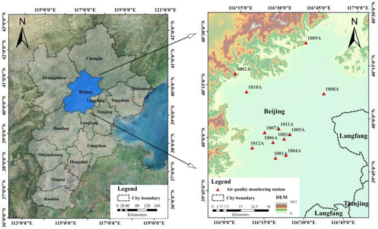
Figure 1.
Study area and the 12 air quality monitoring stations.

Table 1.
Information on the variables of the 12 air quality monitoring stations in Beijing.
2.2. CR-LSTM Model
A previous study [11] demonstrated the significant spatiotemporal correlation between PM2.5 concentrations of air quality monitoring stations in the Beijing–Tianjin–Hebei region. The spatial correlation of 12 air quality monitoring stations is more significant in Beijing (R2 > 0.81) [11]. Therefore, the modeling process should consider the spatiotemporal correlation of air pollution. Additionally, the temporal correlation in individual air quality monitoring stations is also significant through Pearson correlation coefficient analysis. Figure 2 shows the temporal correlation decrease with the increase of the time lag. When the time lag is equal to 12, the Pearson correlation coefficient for 12 air quality monitoring stations is between 0.59 and 0.68. The smaller the time lag, the higher the temporal correlation. The analysis above shows that the spatiotemporal correlation is necessary for the process of modeling. Due to the significant temporal correlation between individual air quality monitoring stations, the combination between recursive strategy and the ConvLSTM network extends the longer-term prediction task and makes up for the shortcoming of the conventional LSTM-based network in long-term prediction tasks. These features allowed us to gain the theoretical basis we needed for constructing the CR-LSTM model.
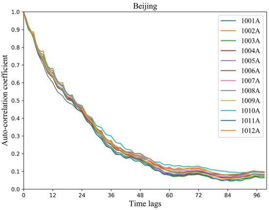
Figure 2.
Temporal correlation for 12 air quality monitoring stations.
2.2.1. The Regional Spatial Station Representation Method
Due to the irregular distribution of the 12 air quality monitoring stations in Beijing (Figure 1), these uneven distributions were not input into the ConvLSTM network. Considering Tobler’s First Law of Geography [3,48], a regional spatial station representation method was used to reorganize the 12 air quality monitoring stations into a regular distribution, using the location relationships (longitude and latitude) to adapt to the data input requirements of the ConvLSTM network, which was viewed as an approximate representation of regional PM2.5 concentration distribution. Additionally, a CNN, as part of a ConvLSTM network and a typical deep learning algorithm, can consider the neighborhood information to extract image features via the convolution kernel operation, which is also used to mine complex spatial relationships around neighborhoods [49,50]. In our study, a CNN was used to capture and quantify the complex spatial correlation of air pollution. Figure 3 shows the reorganized distribution of the 12 air quality monitoring stations in Beijing.
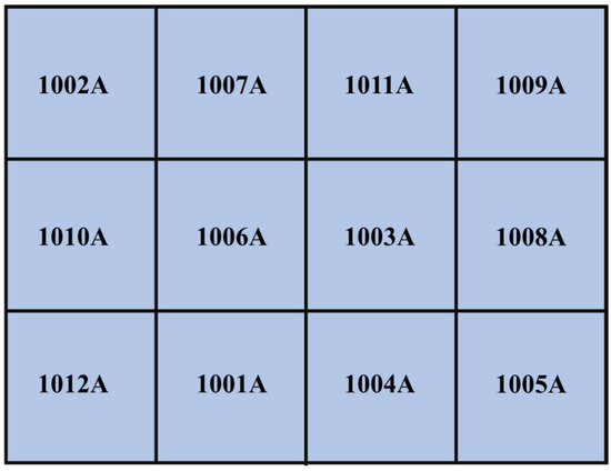
Figure 3.
Reorganized distribution (image) of the 12 air quality monitoring stations in Beijing.
2.2.2. The LSTM Neural Network
The LSTM neural network, a special type of recurrent neural network (RNN), comprised an input layer, an output layer, and a series of memory blocks. Herein, each block had three central units (an input gate, an output gates, and a forget gate) that stored long-term data dependencies. Compared to an RNN, the LSTM model can overcome gradient explosion and disappearance in error backpropagation and is much better at capturing long short-term information. Figure 4 represents the structure of the conventional LSTM model.
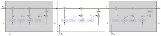
Figure 4.
Structure of the conventional long short-term memory (LSTM) model.
Three gating mechanisms control information transmission in the LSTM model. Herein, the input gate was responsible for inputting the external information into the memory block. The forget and output gates were used for controlling the information that needed to be saved or released from the LSTM block. The conventional LSTM network guided the information transmission through the forget gate ft, the input gate it, and the output gate ot. Xt, Ct, and ht represent the input, internal and external state at time t, respectively. The detailed information transformation in the LSTM block is as follows:
where W and b represent the weights and bias between the transmission layers of the LSTM block; Xt, ht, and Ct are the input, output and memory information at time t; it, ot, and ft represent the input, output, and forget gates, respectively; and (Sigmoid) and tanh are the activation functions, and the formulas are as follow:
2.2.3. The ConvLSTM Neural Network
The conventional LSTM model itself only can capture the temporal correlation of individual air quality monitoring stations. However, the ConvLSTM network, adding a convolution operation to the traditional LSTM model, captures temporal correlations, similarly to the LSTM model, and the spatial correlations among air quality monitoring stations similarly to the CNN, extracting the complex spatiotemporal correlation characteristics of air pollution (Figure 5) [35]. Additionally, the ConvLSTM network can also overcome gradient explosion and disappearance in error backpropagation, resulting in the better capture of long short-term and neighbor information than the conventional LSTM network. Similarly to the LSTM networks, the ConvLSTM network also provides information transmission through the forget gate ft, the input gate it, and the output gate ot. Xt, Ct, and ht refer to the input, internal, and external states at time t, respectively. However, the forget gate ft, the input gate it, and the output gate ot are calculated through states Xt and ht-1 by convolution operation and batch normalization (BN) (Equations (9)–(12)), as well as the internal Ct-1 or Ct. Compared to the conventional LSTM model, the ConvLSTM network is better able to capture longer-term information dependencies. The formulas of information transmission in the ConvLSTM network are as follows:
where Nt is the intermediate variable for the input feature at current moment t, computed by the convolution operation; Wx and Wh are the weight matrixes for the intermediate variable Nt; BN represents the batch normalization operation; Wci and Wcf are the weight matrixes for the variables between internal Ct-1 and input gate it and between Ct-1 and forget gate ft, respectively; Wco is the weight matrixes for the variables between internal Ct and output gate it; bN, bi, bf, bc, and bo are the corresponding biases; and is the matrix operation.
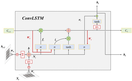
Figure 5.
Structure of the convolutional long short-term memory (ConvLSTM) network.
2.2.4. The CR-LSTM Model
In our study, to allow for spatiotemporal correlations, a spatiotemporal CR-LSTM model was proposed by combining a ConvLSTM neural network and the recursive strategy for predicting future 24-h PM2.5 concentrations for the 12 air quality monitoring stations in Beijing. Figure 6 shows the framework of the proposed CR-LSTM model. Although the ConvLSTM network can predict long short-term prediction tasks, longer-term prediction (up to or greater than 24 h) tasks exhibit poor performance. The recursive strategy was introduced to a ConvLSTM network to extend the long-term prediction task, exploring the prediction potential of said ConvLSTM network in longer-term prediction tasks. A previous study [11] proved that the recursive strategy can improve the conventional LSTM model’s prediction ability in long-term prediction tasks. The CR-LSTM model mainly consists of three parts as follows.
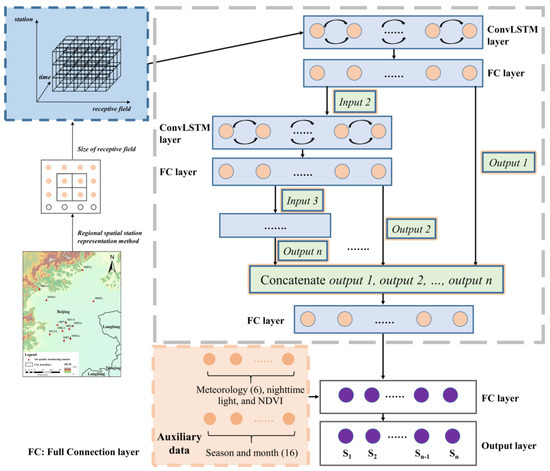
Figure 6.
Framework of the CR-LSTM model. The FC layer refers to the full connection layer, s represents the air quality monitoring station, and n indicates the number of air quality monitoring stations.
Part 1: Spatiotemporal Correlations Configuration
The aim of the first part was to configure the spatiotemporal correlations among air quality monitoring stations and to incorporate them into the ConvLSTM block/unit. The detailed processes were as follows: (1) the spatial correlations of the 12 air quality monitoring stations in Beijing were between 0.81 and 0.97, verifying the necessity of spatial correlations in modeling. The regional spatial station representation method was used to reorganize the 12 air quality monitoring stations in Beijing into a regular distribution using the location relationships (longitude and latitude) to adapt to the data input requirements of the ConvLSTM block. The appropriate receptive field (neighborhood) was configured to quantify the spatial correlation of air pollution. (2) Pearson’s correlation coefficient analysis showed significant temporal correlations for the 12 air quality monitoring stations in Beijing (Figure 2). Since the next prediction results rely on the previous prediction results in the proposed CR-LSTM model, more recursive iterations will result in error accumulation and poor performance. The increase in the number of recursive iterations also increases the number of ConvLSTM units, resulting in expensive computation. Thus, the period of the recursive strategy in the CR-LSTM model affects the model’s performance. In our study, temporal correlations were used to obtain the optimizing time lag r in the recursive prediction task. (3) The ConvLSTM network captured the spatiotemporal correlations of air quality monitoring stations. The configured spatiotemporal correlations were incorporated into the model and were used as the inputs of the ConvLSTM network of the CR-LSTM model.
Part 2: Recursive Prediction Configuration
Part 2 focuses on the crucial component of the proposed CR-LSTM model. The ConvLSTM network can also predict future PM2.5 concentrations. However, it is more suitable for long short-term prediction tasks. Longer-term prediction tasks exhibit poor performance. Previous studies [10,11] have also demonstrated that the accuracy of LSTM-based models decreases significantly as the prediction time interval increases. Longer-term prediction (up to or greater than 24 h) tasks are a challenge for LSTM-based models. The starting point of the proposed CR-LSTM model lowers the model’s prediction error for a longer prediction period of time by combining the recursive strategy and adding the ConvLSTM block, expanding the model’s prediction ability in longer-term prediction tasks. The detailed processes of recursive prediction were as follows: (1) the optimizing time lag r was obtained through Pearson’s correlation coefficient analysis and the appropriate receptive field (neighborhood) was configured from experience. (2) The continuous hourly historical PM2.5 concentrations for the 12 air quality monitoring stations during time interval r and those of the neighboring stations within the N×N window were captured through the bidirectional ConvLSTM layer and the fully connected layer, and the hour-by-hour prediction results within future r hours (output 1) for the 12 air quality monitoring stations were then forecasted. Since the ConvLSTM network generally exhibits good performance for short-term prediction tasks, the time lag r was configured through a trade-off between accuracy and computational expense. Subsequently, the hour-by-hour prediction results within the future r hours (output 1) and the data for the neighboring stations within the N×N window input into the next bidirectional ConvLSTM layer and the fully connected layer, as well as the hour-by-hour prediction results from r to 2*r (output 2) in the future, were obtained. In this iteration, longer-term hour-by-hour prediction results (output 3, …, output n) can be achieved. Finally, the multi-period hour-by-hour prediction results (output 1, output 2, …, output n) were concatenated and input into the next fully connected layer. In the recursive prediction, the selection of time lag r is key to the CR-LSTM model. For specific prediction tasks, a larger r will affect the model’s accuracy in the period of prediction; a smaller r will add to the number of recursive iterations, resulting in error accumulation and expensive computation. In our study, we proposed that the time lag r could be achieved by observing the characteristics of the data and their temporal correlations. In summary, Pearson’s correlation coefficient analysis was one of the tools for obtaining the optimizing time lag r.
Part 3: Auxiliary Data Incorporation
Previous studies [51,52,53] have shown that synoptic conditions are an essential contributor to PM2.5 concentrations. For example, precipitation can wash particles, including PM2.5 particles, reducing the PM2.5 concentration; a higher temperature will significantly dilute surface air pollution, decreasing the PM2.5 concentration. Additionally, the PM2.5 concentration also shows significant seasonal effects: The PM2.5 concentration is highest in the winter and lowest in the summer. Additionally, geographical conditions and human activities also affect the distribution of PM2.5 concentrations. Many studies [10,11,14,34,37] have also incorporated synoptic conditions, geographical conditions, human activities, and season effects into the corresponding models to improve the models’ performance. Our study assumed that the combination of the internal historical change trend derived from the air quality monitoring stations and the dynamic disturbance of the synoptic conditions, geographical conditions, human activities, and seasonal effect together affect future PM2.5 concentrations. Hence, the previous layer’s outputs and auxiliary data (synoptic conditions, geographical conditions, human activities, and seasonal and month effects) were flattened, input into a fully connected layer, and the final hour-by-hour prediction results for the 12 air quality monitoring stations were obtained. The synoptic conditions included wind speed, relative humidity, surface pressure, temperature, precipitation, and sunshine duration; the geographical conditions and human activities were quantified by the NDVI and nighttime light data, respectively. All of the above were normalized by using the min–max scaling method. The seasonal and month effects consisted of the four seasons and 12 months, achieved by one-hot encoding. In the future, more exogenous variables derived from auxiliary data (e.g., topographic data, wind direction, and socio-economic data) will also be incorporated into the corresponding models based on actual business requirements.
In addition, the activation function of the ConvLSTM block is the rectified linear unit (ReLU). The regularization (L2) and dropout (0.1) were used in the fully connected and ConvLSTM layers. The RMSE, the MAE, and the R2 were used to test the model’s performance.
3. Results and Analysis
3.1. Pre-Processing of the Model
The proposed CR-LSTM model could, in theory, be used to predict infinite long-term PM2.5 concentrations via the recursive strategy. However, the temporal correlation of air quality monitoring stations decreases as the time lag increases. Since the following prediction results relied on the previous prediction results, an increasing number of recursive iterations would result in significant error accumulation, especially in the last recursive stage. Generally, the model’s performance in the last recursive stage was the worst of the total recursive prediction process due to the error accumulation. The hour-by-hour prediction results in the last recursive stage may not apply to the actual forecast scenario due to the higher error accumulation. Hence, to improve the model’s performance and to minimize the complexity of the model structure, the mean PM2.5 concentrations in the last recursive stage were set as the model’s output rather than the hour-by-hour prediction results. The detailed recursive processes were as follows. As shown in Figure 6, after configuring the time lag r, it is grouped with the predicted long-term T to form the (T/r) ConvLSTM units. Taking a 24-h (T = 24) prediction task as an example, when time lag r sets to 6, the CR-LSTM model includes six (T/r = 6) ConvLSTM units: the first ConvLSTM unit represents the first set of prediction results (output 1: 1–4 h), the second represents the second set of prediction results (output 2: 5–8 h), the sixth represents the sixth set of prediction results (output 6: The average PM2.5 concentrations from 20 to 24 h), and so on. Through such a recursive prediction, the final continuous long-term prediction sequence is formed.
Ultimately, the time lag r is the key to the CR-LSTM model, determining the time interval of the prediction and the number of recursive iterations. In our study, temporal correlations were used to optimize time lag r in the recursive prediction tasks. The hourly historical PM2.5 concentrations of the 12 air quality monitoring stations in Beijing showed a Pearson’s correlation coefficient between 0.59 and 0.68 when r = 12 (Figure 2). Such a high temporal correlation can be selected as the time lag r of the CR-LSTM model. Hence, in our study, for predicting future 24-h PM2.5 concentrations, the time lag r of the CR-LSTM model was set as 12, the output of the CR-LSTM model included hour-by-hour predictions of the future 1–12 h and the mean PM2.5 concentrations of the future 13–24 h. Tensorflow deep learning lib was then used to build our proposed CR-LSTM model and to train the corresponding model in the Jupyter notebook environment.
3.2. CR-LSTM Model Performance
In our study we collected the hourly historical PM2.5 concentrations and daily mean meteorological data for Beijing from 1 January 2014 to 31 December 2019. Additionally, we also collected the annual nighttime light and NDVI data from 2014 to 2019 and assumed that these do not change within a year. The ratios for the training, verification, and test sets were 60%, 20%, and 20%, respectively. In the ConvLSTM block, the receptive field was set to 2 × 2, and the number of filters was set to 32. The nodes of the fully connected layer in the CR-LSTM model were set to 1000. After determining the network architecture, the CR-LSTM model for 24-h PM2.5 concentration prediction tasks in Beijing was established. The inputs for the CR-LSTM network had five dimensions: the number of input samples, the optimizing time lag r, the width of the image of the ConvLSTM block, the height of the image of the ConvLSTM block, and the number of monitoring stations. The results showed that the model’s performance for the 12 air quality monitoring stations in Beijing was good (R2 = 0.74, RMSE = 18.96 μg/m3, and MAE = 12.89 μg/m3). The details of the performance of the CR-LSTM model for the 12 air quality monitoring stations in Beijing are shown in Table 2 and Figure 7 and Figure 8. The R2 ranged from 0.64 to 0.78, the RMSE from 14.21 to 22.12 μg/m3, and the MAE from 10.16 and 14.75 μg/m3. These results indicate that the proposed CR-LSTM model achieved good performance at both city and individual station scales. According to the daily mean for Level 2 of the CAAQS introduced in 2012 (>75 μg/m3), such performance can assist early warning and management systems of air pollution and has broad application prospects in atmospheric environmental science.
Table 2.
Performance of the CR-LSTM model for the 12 air quality monitoring stations.
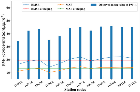
Figure 7.
Performance of the CR-LSTM model and the mean PM2.5 concentrations of the 12 air quality motoring stations in Beijing.
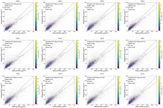
Figure 8.
Correlations between the predicted and observed mean PM2.5 concentrations with the CR-LSTM model for the 12 air quality motoring stations in Beijing.
The hourly historical meteorological data were hard to obtain from the corresponding agencies due to the high data security level in China, resulting in the large time interval overlap in the test set for the existing samples. Using all test samples to evaluate the model’s performance may have brought about a few biases. To minimize these biases and to further explore the proposed CR-LSTM model’s performance at the daily scale, we extracted the specified periods (12–23 h) of the previous day from the test set to predict the daily PM2.5 concentrations on the next day (0–24 h). For example, the daily mean PM2.5 concentration on 1 July 2019 can be predicted from the specified periods (12–23 h) on 30 June 2019. As shown in Figure 9, the R2, RMSE, and MAE for the 12 air quality monitoring stations in Beijing at the daily scale reached 0.8, 15.53μg/m3, and 10.81μg/m3, respectively. Additionally, the R2 of the individual air quality monitoring station at the daily scale ranged from 0.70 to 0.80, the RMSE from 13.57 to 19.98 μg/m3, and the MAE from 9.41 to 13.04 μg/m3 (Figure 10). The results above show that the proposed CR-LSTM model achieved good performance.
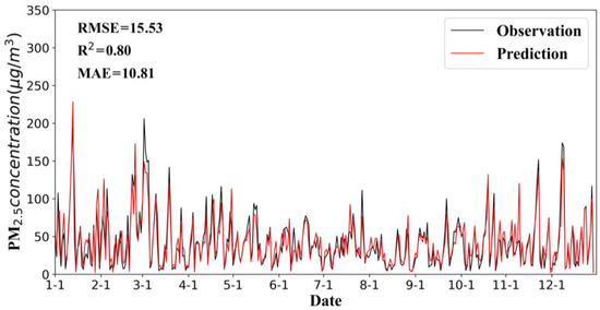
Figure 9.
Comparison between the predicted and observed daily mean PM2.5 concentrations in Beijing from 1 January 2019 to 31 December 2019.
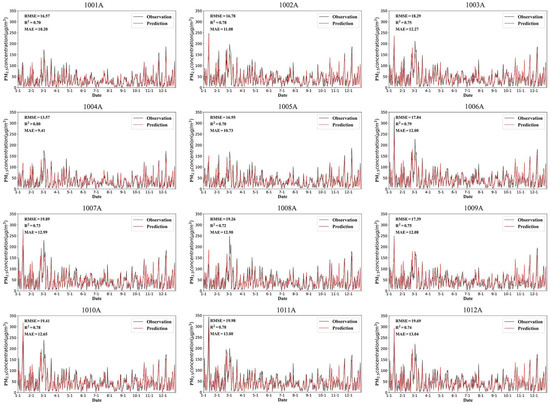
Figure 10.
Comparison between predicted and observed daily mean PM2.5 concentrations of the 12 air quality monitoring stations in Beijing from 1 January 2019 to 31 December 2019.
4. Discussion
4.1. Comparison of the Experiments
Other common models (i.e., MLR, SVR, LSTM, LSTME, and T-LSTME) were selected for comparison with the proposed CR-LSTM model to determine its performance. The MLR, SVR, and LSTM models only consider the hourly historical PM2.5 concentrations; the LSTME and TS-LSTME consider the hourly historical PM2.5 concentrations, as well as the daily mean meteorological data, the geographical conditions, and human activities, but ignore the spatial correlations among air quality monitoring stations. Table 3 shows that the performances of different models at day scale in Beijing, indicating that the proposed CR-LSTM model achieved better performance than the other models. The comparison showed that the deep learning-based models (LSTME, TS-LSTME, and CR-LSTM) were superior to the machine learning-based models (MLR and SVR). Additionally, the comparison between the recursive prediction models (TS-LSTM and CR-LSTM) and the conventional LSTM-based models (LSTME and TS-LSTME) showed that the recursive strategy can significantly improve model performance. The comparison between the CR-LSTM and TS-LSTME models showed that spatial correlation can also improve model performance (RMSE = 18.96 μg/m3 versus 19.87.00 μg/m3; MAE = 12.89 μg/m3 versus 13.24 μg/m3, R2 = 0.74 versus 0.72). Therefore, it is reasonable to assume that the proposed CR-LSTM model provides better PM2.5 concentration prediction than the other models for large-scale regions, such as Jing-Jin-Ji in China.
Table 3.
Comparison of the experiments for the different models for 24-h prediction task in Beijing.
Figure 11 shows the performances (MAE) of the different models for the 12 air quality monitoring stations at the daily scale in Beijing. The results indicate that the proposed CR-LSTM model achieved better performance than the MLR, SVR, LSTM, and LSTME models. Compared to the TS-LSTME model, the proposed CR-LSTM model achieved better accuracy at most air quality monitoring stations.
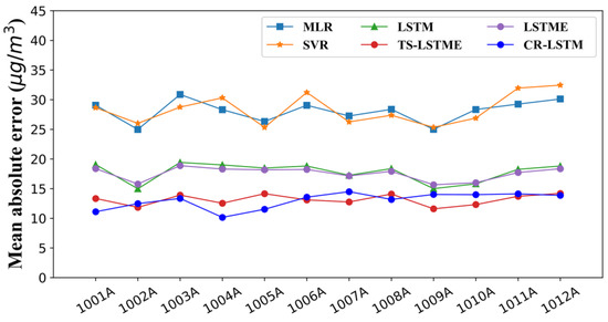
Figure 11.
Performances of other models for the 12 air quality monitoring stations in Beijing.
4.2. Rationality of Time Lag r Derived from the Temporal Correlation
The time lag r, key for the CR-LSTM model, was derived from the temporal correlation analysis of the air quality monitoring stations. Selection of the proper time lag r based on the temporal correlation analysis is worth discussing. A longer time lag r brings about a lower prediction error, particularly in the recursive prediction period, especially in the last time point, while a shorter time lag r brings about an increase in the number of recursive iterations and the complexity of model structure, resulting in error accumulation and expensive computation. Hence, the time lag r was obtained through a trade-off between accuracy and computation expense. In our study, we selected a Pearson’s correlation coefficient value of approximately 0.6 as the time lag r, determined from experience. Artificial judgment may be somewhat subjective. Hence, taking the future 24-h PM2.5 concentrations prediction as an example, we tried to setting multiple time lag values, such as {4, 6, 8, 12, and 24}, in order to validate the rationality of the selected Pearson’s correlation coefficient value of 0.6.
Table 4 shows the performance of the CR-LSTM model for different time lags r in 24-h prediction tasks. Generally, when the time lag r = 12, the proposed CR-LSTM model exhibited better performance than the prediction results with the other time lag value. The results also demonstrated that with an increase in the time lag r, the performance of the proposed CR-LSTM model improved, demonstrating that error accumulation exists in the prediction process along with recursive iterations. Additionally, a smaller r increased the number of ConvLSTM units, thus significantly increasing the training operations. However, the advantage of a smaller r is that it can improve the temporal resolution of the prediction results; For example, when r = 6, the hourly prediction time is 1–18 and the mean PM2.5 concentration is obtained for 19–24 h; when r = 12,the hourly prediction time is 1–12 and the mean PM2.5 concentration is obtained for 13–24 h. Our study provides a Pearson’s correlation coefficient of 0.6 as the reference value of the time lag r in the CR-LSTM model. The time lag r of the CR-LSTM model can also be adjusted based on actual business requirements.
Table 4.
Performance of the CR-LSTM model with different time lags r in 24-h prediction tasks.
4.3. Sensitivity of the Spatiotemporal Dynamics Related to Meteorological Dynamics
Previous studies [51,52,53] have proved that synoptic conditions are an essential contributor to the PM2.5 concentration. For example, Zhang [53] studied the impact of meteorological changes on the PM2.5 mass reduction in key regions in China using the hourly historical PM2.5 concentrations and meteorological data, further guiding us to consider meteorological dynamics in modeling. The leave-one-out method for meteorological data, which involves discarding a meteorological feature, was used to analyze the sensitivity of the spatiotemporal dynamics related to meteorological dynamics for the proposed CR-LSTM model. Due to the reduction in the model’s variables, the fully connected layer nodes in the CR-LSTM model were set to 800. Table 5 shows the model’s performance in different scenes. The results further proved that synoptic conditions affect the model’s performance. Scenes 2–7 of Table 5 show that the RHU and TEM were relatively sensitive to the other synoptic conditions (WS, PRS, PRE, and SSD) for the proposed CR-LSTM model, closely followed by WS and PRE, while the sensitivity of PRS was the lowest. Table 5 (scene 8) demonstrates that the consideration of six sets of meteorological data obtained the best performance in the proposed CR-LSTM model. However, increasing the number of variables leads to complexity of the model structure and computation expense. Hence, sensitivity analysis of variables helps to optimize the model by selecting the corresponding variables through the trade-off of both accuracy and time efficiency.
Table 5.
Performance of the CR-LSTM model in different scenes for the meteorological data.
4.4. Contributions and Limitations
Our study proposed a spatiotemporal CR-LSTM neural network model for predicting PM2.5 concentrations in longer-term prediction tasks by combining a ConvLSTM neural network and the recursive strategy. The proposed CR-LSTM model allows for efficient spatiotemporal correlations of air pollution, while the recursive strategy expands long-term prediction tasks. Longer-term air pollution prediction can also better assist in early warning and air pollution management, showing higher practicalities. The critical contributions of our study are as follows.
(1) We proposed a CR-LSTM model whose essential contribution is to expand longer-term prediction tasks by efficiently considering spatiotemporal correlations and introducing the recursive strategy.
(2) The proposed CR-LSTM model also has strong expansibility and practicability by configuring the proper time lag r derived from temporal correlations.
(3) In the proposed CR-LSTM model, we selected the ConvLSTM block as the basic unit of the CR-LSTM model, improving the model’s performance by efficiently considering spatial autocorrelation. A comparison between the CR-LSTM model and other common models (i.e., MLR, SVR, LSTM, LSTME, and T-LSTME) was used to evaluate the accuracy and stability of the ConvLSTM block of the CR-LSTM model.
However, some limitations still exist in this study and some work needs to be completed in the future. First, our study did not consider spatiotemporal heterogeneity. A previous study [54] proposed geographically and temporally weighted regression (GTWR) to capture spatiotemporal heterogeneity, while the spatiotemporal relationship is still not clear for deep learning-based models. Hence, we will introduce spatiotemporal heterogeneity into the proposed CR-LSTM model in the future [16]. Second, previous studies have also shown a spatiotemporal heterogeneity between PM2.5 concentrations and meteorological features. Our study used meteorological data as auxiliary variables and the spatiotemporal heterogeneity of the meteorological features was ignored. In future research, we will consider the spatiotemporal heterogeneity of meteorological features in modeling. Third, the phenomenon of underestimation of high PM2.5 concentrations and overestimation of low PM2.5 concentrations exists in the many prediction models (see Figure 8 for details), which may bring about some biases. Future research will further analyze the reasons for this phenomenon and improve the model’s performance and practicability. Fourth, we cannot predict if the proposed CR-LSTM model will work for other types of air pollution prediction. In a future study, we will apply the proposed CR-LSTM model to other long-term predictions of air pollution (e.g., O3, NO2, and PM10) to broaden its application. Fifth, our study focused on the validation and analysis of 24-h PM2.5 concentration prediction tasks for the proposed CR-LSTM model. The CR-LSTM will be further applied to longer-term prediction task (e.g., 36, 48, 60, and 72 h) to test the model’s performance in the future. Sixth, the reorganization mapping of the air quality monitoring stations needs to be further optimized by taking into consideration geographical conditions (such as topography, traffic station, and roads network) to improve the model’s performance. Finally, the model was validated based on only 12 air quality monitoring stations in Beijing and so the reliabilities and applicability of the model need further validation. In the next study, we will apply the proposed CR-LSTM model to the case of China and test the model’s performance in large-scale regions.
5. Conclusions
A previous study [11] showed a significant spatiotemporal correlation of the PM2.5 concentrations in the Jing-Jin-Ji Region. The modeling process should consider the spatiotemporal correlation of air pollution efficiently. The manner in which to capture and quantify spatial correlation is also worth discussing. Additionally, conventional LSTM-based models are suitable for long short-term prediction tasks, the longer-term prediction exhibited poor performance. Therefore, expanding longer-term prediction tasks is still challenging. In our study, a spatiotemporal CR-LSTM model was proposed for predicting PM2.5 concentrations by combining a ConvLSTM network and the recursive strategy, thereby expanding the long-term prediction ability. Herein, the ConvLSTM network was used to capture the complex spatiotemporal correlations and to predict the future PM2.5 concentrations; the recursive strategy was used for expanding long-term prediction tasks. The CR-LSTM model was used to realize the future 24-h PM2.5 concentration prediction for 12 air quality monitoring stations in Beijing through the configuration of both the appropriate time lag, derived from the temporal correlations, and spatial neighborhood, including the hourly historical PM2.5 concentrations, daily mean meteorological data, and annual nighttime light and NDVI data. In addition, we also explained the rationality of the combination between the ConvLSTM network and the recursive strategy. Taking the case of 12 air quality monitoring stations in Beijing, the prediction results showed that the proposed CR-LSTM model achieved good performance (all test samples: R2 = 0.74, RMSE = 18.96 μg/m3, MAE = 12.89 μg/m3; daily samples: R2 = 0.8, RMSE = 15.53 μg/m3, MAE = 10.81 μg/m3) and the comparison with the other models also proved the validity and advantage of the proposed CR-LSTM model (see Section 4.1 for details). The conclusions are as follows.
(1) The combination of geographical law, recursive strategy, and deep learning can improve the model’s long-term prediction task performance. The spatiotemporal correlation characteristics of air pollution should be considered in the modeling in long-term prediction tasks.
(2) The combination of a ConvLSTM network and the recursive strategy can improve the model’s performance in expanding longer-term prediction tasks, which provides a new perspective for other deep learning-based methods in longer-term prediction modeling and application.
(3) A spatiotemporal CR-LSTM neural network model was proposed based on a ConvLSTM network and the recursive strategy for PM2.5 concentrations prediction, the essential contribution of which was to expand long-term predicted tasks. The rationality and empirical analysis of the proposed CR-LSTM model were also discussed in detail. The methodological advancements of this study are also applicable to long-term air pollution prediction tasks in other cities or large-scale regions.
Author Contributions
Conceptualization, G.X., W.M., and W.W.; Methodology, W.M. and W.W.; Software, W.M.; Validation, W.W., W.M. and G.X.; Formal Analysis, W.W., W.M., and X.T.; Investigation, W.M., G.X., and W.W.; Resource, G.X.; Data Curation, W.M., and G.X.; Writing, W.W.; Supervision, G.X.; Project Administration, G.X.; Funding Acquisition, G.X. All authors have read and agreed to the published version of the manuscript.
Funding
This study was supported by the Natural Science Foundation of Hubei Province, China (2020CFB274).
Acknowledgments
The authors would like to thank the data provider listed in Table 1 for freely releasing the fundamental data for use. In addition, we sincerely appreciate all the anonymous reviewers for their valuable comments.
Conflicts of Interest
The authors declare no conflict of interest.
References
- Barzeghar, V.; Sarbakhsh, P.; Hassanvand, M.S.; Faridi, S.; Gholampour, A. Long-term trend of ambient air PM10, PM2.5, and O3 and their health effects in Tabriz city, Iran, during 2006–2017. Sustain. Cities Soc. 2020, 54, 101988. [Google Scholar] [CrossRef]
- Kampa, M.; Castanas, E. Human health effects of air pollution. Environ. Pollut. 2008, 151, 362–367. [Google Scholar] [CrossRef] [PubMed]
- Wang, W.; Zhao, S.; Jiao, L.; Taylor, M.; Zhang, B.; Xu, G.; Hou, H. Estimation of PM2.5 concentrations in china using a spatial back propagation neural network. Sci. Rep. 2019, 9, 13788. [Google Scholar] [CrossRef] [PubMed]
- Lelieveld, J.; Evans, J.S.; Fnais, M.; Giannadaki, D.; Pozzer, A. The contribution of outdoor air pollution sources to premature mortality on a global scale. Nature 2015, 525, 367–371. [Google Scholar] [CrossRef]
- Madrigano, J.; Kloog, I.; Goldberg, R.; Coull, B.A.; Mittleman, M.A.; Schwartz, J. Long-term exposure to PM2.5 and incidence of acute myocardial infarction. Environ. Health Persp. 2013, 121, 192–196. [Google Scholar] [CrossRef]
- Zhang, Q.; Jiang, X.; Tong, D.; Davis, S.J.; Zhao, H.; Geng, G.; Feng, T.; Zheng, B.; Lu, Z.; Streets, D.G. Transboundary health impacts of transported global air pollution and international trade. Nature 2017, 543, 705–709. [Google Scholar] [CrossRef]
- Nel, A. Air pollution-related illness: Effects of particles. Science 2005, 308, 804–806. [Google Scholar] [CrossRef]
- National Urban Air Quality Report of China. 2019. Available online: http://www.mee.gov.cn/hjzl/dqhj/cskqzlzkyb/201908/P020190821498490317309.pdf (accessed on 2 July 2019).
- Li, T.; Shen, H.; Zeng, C.; Yuan, Q.; Zhang, L. Point-surface fusion of station measurements and satellite observations for mapping PM2.5 distribution in China: Methods and assessment. Atmos. Environ. 2017, 152, 477–489. [Google Scholar] [CrossRef]
- Wen, C.; Liu, S.; Yao, X.; Peng, L.; Li, X.; Hu, Y.; Chi, T. A novel spatiotemporal convolutional long short-term neural network for air pollution prediction. Sci. Total Environ. 2019, 654, 1091–1099. [Google Scholar] [CrossRef]
- Mao, W.; Wang, W.; Jiao, L.; Zhao, S.; Liu, A. Modeling air quality prediction using a deep learning approach: Method optimization and evaluation. Sustain. Cities Soc. 2020, 65, 102567. [Google Scholar] [CrossRef]
- Geng, G.; Zhang, Q.; Martin, R.V.; van Donkelaar, A.; Huo, H.; Che, H.; Lin, J.; He, K. Estimating long-term PM2.5 concentrations in China using satellite-based aerosol optical depth and a chemical transport model. Remote Sens. Environ. 2015, 166, 262–270. [Google Scholar] [CrossRef]
- Stern, R.; Builtjes, P.; Schaap, M.; Timmermans, R.; Vautard, R.; Hodzic, A.; Memmesheimer, M.; Feldmann, H.; Renner, E.; Wolke, R. A model inter-comparison study focussing on episodes with elevated PM10 concentrations. Atmos. Environ. 2008, 42, 4567–4588. [Google Scholar] [CrossRef]
- Wang, J.; Bai, L.; Wang, S.; Wang, C. Research and application of the hybrid forecasting model based on secondary denoising and multi-objective optimization for air pollution early warning system. J. Clean. Prod. 2019, 234, 54–70. [Google Scholar] [CrossRef]
- Pan, L.; Sun, B.; Wang, W. City air quality forecasting and impact factors analysis based on grey model. Procedia Engineering. 2011, 12, 74–79. [Google Scholar] [CrossRef]
- Li, T.; Shen, H.; Yuan, Q.; Zhang, L. Geographically and temporally weighted neural networks for satellite-based mapping of ground-level PM2.5. ISPRS J. Photogramm. Remote Sens. 2020, 167, 178–188. [Google Scholar] [CrossRef]
- Yuan, Q.; Shen, H.; Li, T.; Li, Z.; Li, S.; Jiang, Y.; Xu, H.; Tan, W.; Yang, Q.; Wang, J.; et al. Deep learning in environmental remote sensing: Achievements and challenges. Remote Sens. Environ. 2020, 241, 111716. [Google Scholar] [CrossRef]
- Lv, B.; Cai, J.; Xu, B.; Bai, Y. Understanding the rising phase of the PM2.5 concentration evolution in large China cities. Sci. Rep. 2017, 7, 46456. [Google Scholar] [CrossRef]
- Gupta, P.; Christopher, S.A. Particulate matter air quality assessment using integrated surface, satellite, and meteorological products: 2. A neural network approach. J. Geophys. Res. Atmos. 2009, 114, 1–14. [Google Scholar] [CrossRef]
- Zhang, G.; Lu, H.; Dong, J.; Poslad, S.; Li, R.; Zhang, X.; Rui, X. A framework to predict high-resolution spatiotemporal PM2.5 distributions using a deep-learning model: A case study of Shijiazhuang, China. Remote Sens. 2020, 12, 2825. [Google Scholar] [CrossRef]
- Fan, Z.; Zhan, Q.; Yang, C.; Liu, H.; Bilal, M. Estimating PM2.5 concentrations using spatially local Xgboost based on full-covered SARA AOD at the urban scale. Remote Sens. 2020, 12, 3368. [Google Scholar] [CrossRef]
- Shen, H.; Jiang, Y.; Li, T.; Cheng, Q.; Zeng, C.; Zhang, L. Deep learning-based air temperature mapping by fusing remote sensing, station, simulation and socioeconomic data. Remote Sens. Environ. 2020, 240, 111692. [Google Scholar] [CrossRef]
- Wan, R.; Mei, S.; Wang, J.; Liu, M.; Yang, F. Multivariate temporal convolutional network: A deep neural networks approach for multivariate time series forecasting. Electronics 2019, 8, 876. [Google Scholar] [CrossRef]
- Qi, Y.; Li, Q.; Karimian, H.; Liu, D. A hybrid model for spatiotemporal forecasting of PM2.5 based on graph convolutional neural network and long short-term memory. Sci. Total Environ. 2019, 664, 1–10. [Google Scholar] [CrossRef]
- Shen, H.; Li, T. Progress of remote sensing mapping of atmospheric PM2.5. Acta Geodaetica et Cartographica Sinica 2019, 48, 1426–1635. [Google Scholar]
- Han, L.; Zhao, J.; Gao, Y.; Gu, Z.; Xin, K.; Zhang, J. Spatial distribution characteristics of PM2.5 and PM10 in Xi’an city predicted by land use regression models. Sustain. Cities Soc. 2020, 61, 102329. [Google Scholar] [CrossRef] [PubMed]
- Stadlober, E.; Hörmann, S.; Pfeiler, B. Quality and performance of a PM10 daily forecasting model. Atmos. Environ. 2008, 42, 1098–1109. [Google Scholar] [CrossRef]
- Perez, P.; Reyes, J. An integrated neural network model for PM10 forecasting. Atmos. Environ. 2006, 40, 2845–2851. [Google Scholar] [CrossRef]
- Suárez Sánchez, A.; García Nieto, P.J.; Riesgo Fernández, P.; Del Coz Díaz, J.J.; Iglesias-Rodríguez, F.J. Application of an SVM-based regression model to the air quality study at local scale in the Avilés urban area (Spain). Math. Comput. Model. 2011, 54, 1453–1466. [Google Scholar] [CrossRef]
- Gariazzo, C.; Carlino, G.; Silibello, C.; Renzi, M.; Finardi, S.; Pepe, N.; Radice, P.; Forastiere, F.; Michelozzi, P.; Viegi, G.; et al. A multi-city air pollution population exposure study: Combined use of chemical-transport and random-forest models with dynamic population data. Sci. Total Environ. 2020, 724, 138102. [Google Scholar] [CrossRef] [PubMed]
- Danesh Yazdi, M.; Kuang, Z.; Dimakopoulou, K.; Barratt, B.; Suel, E.; Amini, H.; Lyapustin, A.; Katsouyanni, K.; Schwartz, J. Predicting fine particulate matter (PM2.5) in the greater London area: An ensemble approach using machine learning methods. Remote Sens. 2020, 12, 914. [Google Scholar] [CrossRef]
- Schneider, R.; Vicedo-Cabrera, A.M.; Sera, F.; Masselot, P.; Stafoggia, M.; de Hoogh, K.; Kloog, I.; Reis, S.; Vieno, M.; Gasparrini, A. A satellite-based spatio-temporal machine learning model to reconstruct daily PM2.5 concentrations across Great Britain. Remote Sens. 2020, 12, 3803. [Google Scholar] [CrossRef]
- Zhou, Q.; Jiang, H.; Wang, J.; Zhou, J. A hybrid model for PM2.5 forecasting based on ensemble empirical mode decomposition and a general regression neural network. Sci. Total Environ. 2014, 496, 264–274. [Google Scholar] [CrossRef]
- Chang-Hoi, H.; Park, I.; Oh, H.; Gim, H.; Hur, S.; Kim, J.; Choi, D. Development of a PM2.5 prediction model using a recurrent neural network algorithm for the Seoul metropolitan area, Republic of Korea. Atmos. Environ. 2021, 245, 118021. [Google Scholar] [CrossRef]
- Abirami, S.; Chitra, P. Regional air quality forecasting using spatiotemporal deep learning. J. Clean. Prod. 2021, 283, 125341. [Google Scholar] [CrossRef]
- Zhang, B.; Zou, G.; Qin, D.; Lu, Y.; Jin, Y.; Wang, H. A novel Encoder-Decoder model based on read-first LSTM for air pollutant prediction. Sci. Total Environ. 2021, 765, 144507. [Google Scholar] [CrossRef] [PubMed]
- Ma, J.; Ding, Y.; Cheng, J.C.P.; Jiang, F.; Gan, V.J.L.; Xu, Z. A Lag-FLSTM deep learning network based on Bayesian optimization for multi-sequential-variant PM2.5 prediction. Sustain. Cities Soc. 2020, 60, 102237. [Google Scholar] [CrossRef]
- Yan, R.; Liao, J.; Yang, J.; Sun, W.; Nong, M.; Li, F. Multi-hour and multi-site air quality index forecasting in Beijing using CNN, LSTM, CNN-LSTM, and spatiotemporal clustering. Expert Syst. Appl. 2021, 169, 114513. [Google Scholar] [CrossRef]
- Leng, X.; Wang, J.; Ji, H.; Wang, Q.; Li, H.; Qian, X.; Li, F.; Yang, M. Prediction of size-fractionated airborne particle-bound metals using MLR, BP-ANN and SVM analyses. Chemosphere 2017, 180, 513–522. [Google Scholar] [CrossRef]
- Li, X.; Peng, L.; Yao, X.; Cui, S.; Hu, Y.; You, C.; Chi, T. Long short-term memory neural network for air pollutant concentration predictions: Method development and evaluation. Environ. Pollut. 2017, 231, 997–1004. [Google Scholar] [CrossRef]
- Zhou, Y.; Chang, F.; Chang, L.; Kao, I.; Wang, Y. Explore a deep learning multi-output neural network for regional multi-step-ahead air quality forecasts. J. Clean. Prod. 2019, 209, 134–145. [Google Scholar] [CrossRef]
- Huang, C.; Kuo, P. A deep CNN-LSTM model for particulate matter (PM2.5) forecasting in Smart Cities. Sensors 2018, 18, 2220. [Google Scholar] [CrossRef] [PubMed]
- Li, T.; Shen, H.; Yuan, Q.; Zhang, X.; Zhang, L. Estimating ground-level PM2.5 by fusing satellite and station observations: A geo-intelligent deep learning approach. Geophys. Res. Lett. 2017, 44, 911–985, 993. [Google Scholar] [CrossRef]
- Li, T.; Wang, Y.; Yuan, Q. Remote sensing estimation of regional NO2 via space-time neural networks. Remote Sens. 2020, 12, 2514. [Google Scholar] [CrossRef]
- Shi, X.; Chen, Z.; Wang, H.; Yeung, D.; Wong, W.; Woo, W. Convolutional LSTM network: A machine learning approach for precipitation nowcasting. Adv. Neural Inf. Process. Syst. 2015, 28, 802–810. [Google Scholar]
- Ministry of Ecology and Environment of the People’s Republic of China. Ambient Air Quality Standards. 2012. Available online: http://www.mee.gov.cn/ywgz/fgbz/bz/bzwb/dqhjbh/dqhjzlbz/201203/t20120302_224165.shtml (accessed on 29 February 2012).
- Centre for Research on Energy and Clean Air. 2020. Air Pollution in China (2019). Available online: https://energyandcleanair.org/wp/wp-content/uploads/2020/01/CREA-brief-China2019-Zh.pdf (accessed on 31 January 2020).
- Tobler, W.R. A computer movie simulating urban growth in the Detroit region. Econ. Geogr. 1970, 46, 234–240. [Google Scholar] [CrossRef]
- He, J.; Li, X.; Yao, Y.; Hong, Y.; Jinbao, Z. Mining transition rules of cellular automata for simulating urban expansion by using the deep learning techniques. Int. J. Geogr. Inf. Sci. 2018, 32, 2076–2097. [Google Scholar] [CrossRef]
- Wu, C.; Li, Q.; Hou, J.; Karimian, H.; Chen, G. PM2.5 concentration prediction using convolutional neural networks. Sci. Surv. Mapp. 2018, 43, 68–75. [Google Scholar]
- Xu, G.; Jiao, L.; Zhao, S.; Cheng, J. Spatial and temporal variability of PM2.5 concentration in China. Wuhan Univ. J. Nat. Sci. 2016, 21, 358–368. [Google Scholar] [CrossRef]
- Xu, G.; Jiao, L.; Zhang, B.; Zhao, S.; Ma, Y.; Gu, Y.; Liu, J.; Tang, X. Spatial and temporal variability of the PM2.5/PM10 ratio in Wuhan, Central China. Aerosol Air Qual. Res. 2017, 17, 1–11. [Google Scholar] [CrossRef]
- Zhang, X.; Xu, X.; Ding, Y.; Liu, Y.; Zhang, H.; Wang, Y.; Zhong, J. The impact of meteorological changes from 2013 to 2017 on PM2.5 mass reduction in key regions in China. Sci. China Earth Sci. 2019, 62, 1885–1902. [Google Scholar] [CrossRef]
- Huang, B.; Wu, B.; Barry, M. Geographically and temporally weighted regression for modeling spatio-temporal variation in house prices. Int. J. Geogr. Inf. Sci. 2010, 24, 383–401. [Google Scholar] [CrossRef]


Publisher’s Note: MDPI stays neutral with regard to jurisdictional claims in published maps and institutional affiliations. |
© 2021 by the authors. Licensee MDPI, Basel, Switzerland. This article is an open access article distributed under the terms and conditions of the Creative Commons Attribution (CC BY) license (http://creativecommons.org/licenses/by/4.0/).