Abstract
Convolutional neural networks (CNNs) have been widely used in change detection of synthetic aperture radar (SAR) images and have been proven to have better precision than traditional methods. A two-stage patch-based deep learning method with a label updating strategy is proposed in this paper. The initial label and mask are generated at the pre-classification stage. Then a two-stage updating strategy is applied to gradually recover changed areas. At the first stage, diversity of training data is gradually restored. The output of the designed CNN network is further processed to generate a new label and a new mask for the following learning iteration. As the diversity of data is ensured after the first stage, pixels within uncertain areas can be easily classified at the second stage. Experiment results on several representative datasets show the effectiveness of our proposed method compared with several existing competitive methods.
1. Introduction
Remote sensing (RS) change detection is used to detect changes in a particular area on the surface of the Earth at different times. It provides references for urban planning [1], environment monitoring [2,3], and disaster assessment [4,5]. Several kinds of RS images exist—namely, optical RS images, electro-optical imaging images, and synthetic aperture radar (SAR) images. Among these images, SAR images are widely used because of their independence in atmospheric and sunlight conditions. However, SAR images often have the characteristics of low resolution and low contrast, and suffer from high speckle noise. Over the decades, although many excellent change detection methods have been proposed, how to detect changes accurately and efficiently remains challenging.
Many change detection algorithms for RS images can be shared, to some extent. However, some differences in characteristics exist among RS images. First, an RS image based on optics has abundant texture information, but most SAR images are single bands with relatively low resolutions and less texture information. Second, the types of noise are different. SAR images often have strong speckle noise, while optical RS images often have other types of noise, such as Gaussian noise, impulse noise, and periodic noise. Finally, compared with the optical RS dataset, very few SAR datasets are available for change detection. Usually, a dataset contains only one pair of temporal images. Moreover, for different datasets, the noise distribution and types of ground, such as sea ice, forest, and city, are different. In addition, the image size of the SAR dataset is very small, being usually only a few hundred pixels in length and width. Thus, achieving end-to-end learning for SAR datasets is more difficult. A detailed comparison will be made for optical and SAR images in this paper.
1.1. Traditional Methods
Traditional RS image change detection methods can be divided into two categories: pixel-based and object-based [6]. For RS images, pixel-based methods directly compare the same pixels in different images and then obtain the detection result by using the threshold method or clustering method. Early pixel-based algorithms often take a single pixel as a unit without considering spatial information. So far, many excellent methods have been proposed, such as algebra-based methods [7,8], transformation-based methods [9,10], and classification-based methods [11,12]. Methods for SAR images follow the same ideas as the above RS methods. However, different from RS images, SAR images contain serious speckle noise, which leads to different ideas when making difference images (DI). Three main steps exist for the pixel-based method: (i) preprocessing images, (ii) obtaining DI from inputs, and (iii) processing DI to obtain the final change detection result. The purpose of preprocessing was introduced before. To obtain good DI, log-ratio operator [13] for SAR images is widely adopted because of its excellent performance in suppressing speckle noise. Other kinds of operators are also used in some studies, such as the mean ratio operator [14], the Gauss ratio operator [15], and the neighborhood ratio operator [16]. To obtain change detection results from DI, thresholding approaches [17,18] and clustering approaches [19,20,21] are popularly used. However, because these methods do not make full use of spatial information, it always leads to noisy output. Later, some methods introduced the information of surrounding pixels to weaken this defect, such as spectral–spatial feature extraction methods [16] and random fields-based methods [22]. These improved algorithms may be effective for low-to medium-resolution imagery but always fail to detect for high-resolution imagery [23,24]. Therefore, numerous object-based methods have been proposed to effectively utilize more texture and spatial information [25,26]. The analysis unit used to detect could be patches or superpixels. Thus, noise and small false change area can be effectively eliminated, and the computing time is reduced. However, the change detection accuracy is highly dependent on segmentation algorithms. An exhaustive survey of object-based methods is presented in references [27,28].
1.2. AI-Based Methods
Recently, AI-based methods have achieved great success in the field of image processing. In the field of RS change detection, the accuracy of AI-based methods is far higher than that of traditional methods, especially for SAR images. Given one pair of bitemporal SAR images, the purpose of change detection is to detect changes between images. Different from SAR datasets, some optical RS datasets, such as the ONERA dataset [29], SECOND dataset [30], and Google dataset [31], contain enough images for training. However, it is difficult to learn in an end-to-end and supervised way for SAR images. This is because heavy manual work is required for pixel-wise annotation, which leads to the available datasets are very lacking. Thus, unsupervised methods have gained great attention due to the lack of datasets for SAR images [32]. The first step for unsupervised learning is to select reliable pixels as labels. However, the selected labels are irregularly distributed in the change map, making it difficult to learn in an end-to-end way.
In this article, we divide unsupervised methods into three categories: (1) pixel-based methods, (2) patch/superpixel-based methods, and (3) image-based methods. Pixel-based methods classify only one pixel at a time. Superpixel-based methods first segment images into blocks and then learn features transformed from the blocks to obtain the final results. The hypothesis of using this kind of method is that pixels within the same segmented blocks have similar characters. Different from superpixel-based methods, patch-based methods first crop patches with regular shapes from SAR images and then learn in the form of image segmentation. Image-based methods directly use the whole images as input and classify all pixels at the same time.
1.2.1. Pixel-Based Methods
This kind of method is suitable for dealing with tasks when labels are distributed irregularly within an image. Numerous methods based on convolutional neural network (CNN) [33,34], deep neural network (DNN) [35,36], and autoencoder (AE) [37,38] have been proposed. In reference [37], features were extracted by wavelet transform and then distinguished by a stacked autoencoder (SAE) network. Reference [39] utilized restricted Boltzmann machine (RBM) to calculate difference relations of vectors transformed from raw images. In reference [35], DNN were designed to learn difference relations among features extracted from saliency-guided change maps. However, all the above methods can deal with 1D features only, resulting in the loss of spatial information. To overcome this drawback, algorithms based on 2D features are proposed. This kind of method trains the network in the form of patches but classifies only the central pixel of each patch at a time. In reference [40], patches were cropped from raw images and inputted into the designed PCANet to learn the change relations. References [33,41] used small patches from raw images centering at target pixels as input. Feature extraction and classification procedures are both processed by CNNs. In reference [42], small patches centering at target pixels were cropped from raw images. Then, SAE is applied to transform patches into feature maps, which will be inputted into a designed CNN to be further classified. However, only the central pixel is classified for the above 2D patch-based methods. Too many training samples are generated, resulting in heavy computational cost. Moreover, the patches used in the above methods are usually small, which leads to the loss of local–global information.
1.2.2. Patch/Superpixel-Based Methods
Superpixel-based methods are widely used in the field of change detection of RS images. The shapes of superpixels are irregular, which is why superpixels are often transformed into 1D features. Thus, networks such as multilayer perceptron [27] and AE [38,43] are popularly used. Reference [44] first segmented images into superpixels and then utilized the stacked contractive autoencoder network to classify pixels. Reference [43] generated multiscale superpixels by using DI-guided segmentation. Then, superpixels were vectorized and inputted into the neural network to be further classified. However, the above methods must transform 2D images into 1D features, resulting in the loss of spatial information. To overcome the drawback, a few methods based on patches have been proposed to solve the problem. Reference [45] used a rectangular patch containing the maximum contour of the superpixel as the input, which preserves 2D spatial information. However, given the irregular shape of the superpixels, excessive interference information was mixed into the rectangular box, which seriously influences the classification result. Reference [46] converted superpixels into 1D vectors first, and then, the vector converted back to 2D patches with a regular shape, which retained the spatial information to some extent. However, the above patch-based methods cannot learn in an end-to-end way. Reference [32] utilized transfer learning to train on other datasets and test on the target dataset. However, the result was suboptimal, because the distribution and density of noise were different for different SAR datasets. For optical RS images, references [47] and [48] directly cropped patches from datasets and learned in an end-to-end way. So far, annotated datasets are still few, thus posing difficulty for learning in an end-to-end way on patch or image levels.
1.2.3. Image-Based Methods
Image-based methods have high classification efficiency in classifying all pixels at one time. Numerous methods have been proposed. Reference [49] utilized CNN to extract features first, and then low-rank decomposition and threshold operation were performed to obtain the result. References [50,51,52,53] utilized deep Siamese convolutional network to extract deep features for images separately. The distances between features were then calculated. The final change maps were obtained by applying a threshold function. In reference [54], the pixels were transformed into 1D features by the neural network, and a cluster algorithm was designed to divide features into two categories. However, all the above methods need complex postprocessing procedures, and the pretrained network may not be suitable for extract discriminative features. Few methods that do not need post-processing have been proposed. Reference [55] utilized transfer learning to train the network on other datasets and transfer learned deep knowledge to sea ice analysis. However, the characteristics of the sea ice dataset were different from ground datasets, and the result was suboptimal. For optical RS images, reference [56] used a CNN named UNet++ to fuse multilayer features; this approach outperforms other state-of-the-art CD methods. Reference [57] designed a CNN named SiU-Net for building change detection tasks and outperforms many building extraction methods.
From the above analysis, several problems exist for SAR image change detection tasks. First, due to the irregular distribution of labels, pixel-based methods and superpixel-based methods are popularly used. However, the pixel-based method is time-consuming, and the superpixel-based method is deeply dependent on the segmentation result. When based on superpixels, most methods transform 2D images into 1D features, tending to lose 2D spatial information. Second, for patch-based and image-based methods, the positions of the labels are unevenly distributed in the image. Thus, creating a label map with regular shapes is difficult, thereby posing challenges to achieving end-to-end deep learning. Third, when selecting reliable labels at the pre-classification stage, all the above methods cannot balance diversity and noise. When data diversity is ensured, more noise is mixed into the labels. Similarly, when making training data with less noise, the diversity of data is lost. This situation presents a hard trade-off option.
To solve the above issues, we propose an unsupervised patch-based method without manual labeling. In our proposed method, a mask function is designed to map labels with irregular shapes into a regular map. The method learns the features of changes in an iterative way, and the diversity of data is restored gradually. Thus, the influences of noise on the results of change detection are alleviated. The main contributions of this paper are as follows:
- Change detection through a patch-based approach. A mask function is designed to change labels with irregular shapes into a regular map such that the network can learn patches in an end-to-end way.
- Learning change features iteratively. A two-stage updating strategy is designed to enrich data diversity and suppress noise through iterative learning.
2. Methodology
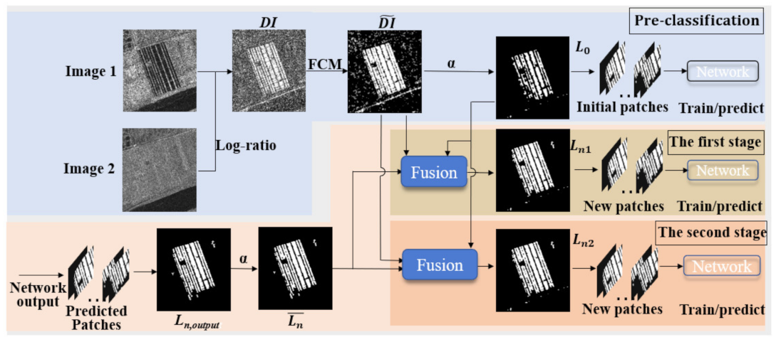
This section presents the mask-based and iterative network. The proposed method generally consists of three parts: pre-classification and patch generation, network and loss function, and two-stage updating strategy. The function of the first part is to generate reliable training samples and labels. The second part is the key to achieving end-to-end learning. The last part enables the network to learn iteratively such that the truly changed areas are recovered gradually. The workflow of the proposed method is shown in Figure 1.

Figure 1.
Overall workflow of the proposed network. Training samples and the designed mask are first generated from bi-temporal images. With the existence of a mask, the network based on UNet can learn in an end-to-end way, ignoring the irregular shape of labels. Through iteratively learning, the newly generated change map is further processed to obtain new label and mask, which will be used in the next learning iteration.
2.1. Pre-Classification and Patch Generation
The main purpose of this section is to generate highly reliable samples as training data. A mask function will also be introduced. The function of the mask is to map irregular labels into a regular map such that the network can directly learn in an end-to-end way. Generally, this section consists of three parts: (1) label pre-classification, (2) mask generation, and (3) patch generation.
2.1.1. Label Pre-Classification
The main purpose of this part is to generate highly reliable labels. Speckle noise in the SAR image is multiplicative noise; thus, the log-ratio operator is adopted to transform multiplicative noise into additive noise and obtain DI. For multitemporal images, I1 and I2, the DI can be denoted as follows:
where 1 < i < WD and 1 < j <HT. WD and HT are the width and height of the images, respectively.
The noise in DI is greatly suppressed, as shown in Figure 2. However, some isolated noise still exists. Thus, the FCM (fuzzy c-means algorithm) clustering algorithm is further utilized to generate reliable labels. The FCM algorithm is popularly used in the field of change detection of SAR images and proven to be effective to suppress speckle noise [20,21]. Pixels in DI will be divided into three categories, namely, changed, unchanged, and uncertain category. The newly clustered map is denoted as . After this operation, noise in changed and unchanged areas is greatly suppressed. However, it is still unsuitable for network learning, because little isolated noise still exists in the newly clustered map. Thus, operations are needed to further eliminate isolated noise and choose reliable labels.
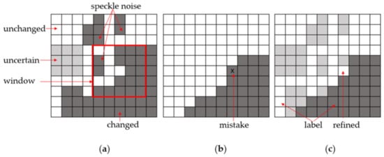
Figure 2.
Illustration of the filtering function. (a) The image obtained by clustering operation. (b) The image obtained by Equation (3). (c) Changed and unchanged pixels are selected as labels. The image is first filtered by Equation (3) to eliminate the speckle noise, as shown in (b), then refined to obtain the label by Equation (4), as shown in (c). Pixels in grey color in (c) contain speckle noise and truly changed pixels, which will be classified by learning.
First, because only very reliable pixels are selected, pixels in the uncertain areas are abandoned. To be brief, we let values of changed, unchanged, and uncertain pixels be 1, 0, and 0.5, respectively. Second, a filter with a size of 5 × 5 is utilized to eliminate speckle noise in the .
where n ∈ {0, 1, …., N}, and N is the total number of iterations. The value of γ is between 0 and 1. α is a threshold to choose reliable labels. At the pre-classification stage, n is 0. denotes the position of neighbor pixel of center pixel (x, y) in the images. denotes a filtered image. The values of α and W are set to 0.7 and 5 at the pre-classification stage, because speckle noise always appears as little blocks, and a larger window size and α can be more effective. As shown in Figure 2, speckle noise can be eliminated with the proposed filter function. However, truly changed pixels are also eliminated by this function such that the diversity of data is lost. To solve this issue, two operations are presented. First, the values of α and W are set to 0.7 and 5, respectively, only at the pre-classification stage. Second, we design an iterative network to gradually restore the diversity of data, which will be introduced later.
Third, as shown in Figure 2, the value of the center pixel is changed to 1 after the filter function, which is incorrect. Thus, a post-processing procedure is designed to correct this mistake. Unchanged pixels in are used to correct the above error pixels such that the changed labels are finally generated. Furthermore, to select unchanged labels, pixels in with values of 0 are chosen. This is because speckle noise often leads to a strong change between two images, and very little noise exists within unchanged areas after the FCM algorithm is used.
where is the newly generated change map, and pixels in with values of 1 will be selected as changed labels. Finally, changed and unchanged pixels in are selected as labels for learning. However, pixels with values of 0.5 still exist in such that learning based on patches is difficult. Therefore, a mask function is introduced to solve the issue.
2.1.2. Mask Generation
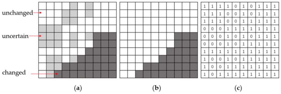
The generated label still contains three categories, and the positions of selected labels are distributed randomly in the map. To make it suitable for the binary task, we directly let pixels with a value of 0.5 be 0. However, pixels with a value of 0.5 are wrong labels. To eliminate the impact of this operation, a mask function that cooperates with loss function is designed. The pixels in the mask, as shown in Figure 3c, are assigned as 0 if values of pixels in are 0.5. In addition, the pixels selected as labels are assigned as 1 in the mask.
where n ∈{0, 1,…, N}, and N is the total iteration number. At the pre-classification stage, n is 0. Mn and Ln will be updated along with the iterative learning. The process of generating labels can be seen in Figure 4.
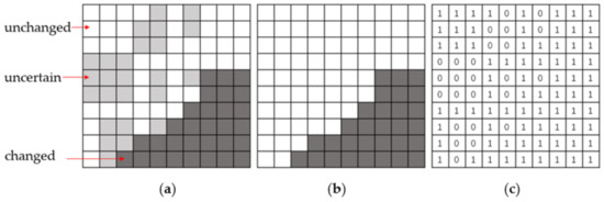
Figure 3.
(a) Pre-classification result (Ln,pre). Pixels in white and black colors are selected labels. (b) The final label with a regular shape. (c) The mask. Pixels belonging to the changed and unchanged categories in (a) are weighted to be 1. Pixels belonging to the uncertain category are weighted to be 0.
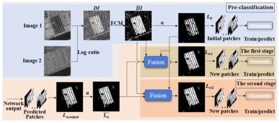
Figure 4.
Illustration of label generation operations for each stage. At the pre-classification stage, the initial label L0 is generated from synthetic aperture radar (SAR) images and contains the least data diversity. Patches are predictions of the designed network. All patches will be spliced into a map, and the map will be processed to be a new label for the next learning iteration. Ln1 is the label generated from the stage one updating process, while Ln2 is the label generated from the stage two updating process.
2.1.3. Patch Generation
With the existence of the mask function, our proposed method can learn based on patches, which can greatly save the computational cost. Different from pixel-based methods [33,34,41], our method classifies all pixels within a patch instead of classifying only the center pixel of a patch. Thus, memory efficiency is improved, and patches are easier to crop. Unlike superpixel-based methods, our patch-based method is not affected by segmentation error. Moreover, unlike existing patch and image-based methods, our method learns in an end-to-end way by using the mask function.
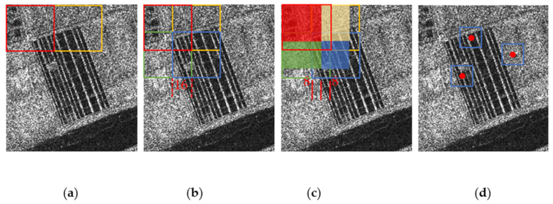
When patches are cropped, the classification results at the edges of patches tend to be inferior because of the influence of padding and pooling operations in the CNN. Instead, as shown in Figure 5b, an overlap with 16 pixels is adopted. The size of overlap is set to 16, because the network contains four pooling layers, which will greatly influence the classification results of the eight pixels near the edge. As shown in Figure 5b, the rectangles in different colors represent cropped patches. As shown in Figure 5c, eight pixels near the edges of each patch are discarded, and the blocks in different colors represent the change detection results that are chosen to be stitched together into the whole change map.

Figure 5.
Method of cropping patches from images: (a) crop without overlap and (b) crop with overlap of 16 pixels. (c) Blocks in different colors will be chosen as final results and stitched together into a final change map. (d) Other patch-based SAR image change the detection task (classifying only the center pixel for a patch).
2.2. Proposed CNN and Loss Function
2.2.1. Proposed CNN
The feature fusion network is widely used today. Reference [58] introduced an embedded block residual network, which uses a multilayer fusion strategy to fully exploit feature information to reconstruct a super-resolution image. Reference [56] adopted UNet++, a dense feature fusion network, to fuse almost every layer of the network. Similar to UNet++, reference [55] constructed a dense block to fuse every layer inside the block. All the above methods obtain remarkable results. Inspired by the above methods, we build a simpler network, as shown in Figure 6. A comparison with the above methods shows that the backbone of the network is similar to the UNet [59] architecture. The number of layers and the size of input are different. Besides, to fully exploit semantic information of different layers, features in every decoder layer are fused in our network. Unlike other CNN-based methods [33,41] for SAR change detection, our network is deeper, such that the semantic information is fully exploited. Moreover, the proposed method is based on patches and learns in an end-to-end way.

Figure 6.
Illustration of the proposed network. Two kinds of fusion functions are utilized.
The network has two kinds of fusion operations. First, skip connection is used in its backbone to the fuse encoder and decoder layers. As shown in Figure 6, feature map X5 can be obtained by using a concatenation function.
where g denotes a deconvolution function. Thus, features from shallow layers and deep layers are fused. Next, to obtain more discriminative features, features in the decode layers are further fused, because speckle noise is unlikely to be strong in every layer. After fusion, more discriminative features can be automatically learned by the network. To complete the fusion, features in the decoder layers are first enlarged to their original sizes and then further extracted to be new features—namely, F1, F2, F3, and F4. Finally, the fused feature map F5 is obtained by using a concatenation function. The details of the network can be found in Table 1.

Table 1.
Details of the network.
2.2.2. Loss Function
In this paper, the binary cross entropy (BCE) loss is adopted in the classification task. As introduced before, it is one of the key functions to accomplish learning process and can be described as
where , , and represent the BCE loss, label, and prediction, respectively. is the weight coefficient that is always used to deal with the problem of sample imbalance. In this paper, we switched to another method, using this weighting coefficient to guarantee that unclassified pixels do not participate in the training process. If the loss of unclassified pixels is 0, then the influence of unclassified pixels is eliminated. Thus, we design a mask . When training, mask Mn and loss function ln can be combined to satisfy the above assumption.
2.3. Two-Stage Updating Strategy
Learning in an iterative way was previously used in some tasks. Reference [60] utilized an autoencoder to extract image features and then used an iterative method to train another neural network. Reference [61] used an iterative approach to train an optical flow estimation network and achieves SOTA result. Inspired by reference [61], this paper introduces a two-stage label updating mechanism to solve the problem of data diversity and noise being difficult to balance. Unlike the above iterative network, the purpose of the proposed method is to gradually restore data diversity instead of minimizing residual error.
Another purpose of iterative learning is to suppress speckle noise. When a label for existing AI-based methods is generated at the pre-classification stage, solving the problem of balancing data diversity and noise is difficult. First, for a particular dataset, more noisy pixels are introduced when data diversity is ensured. Second, for different datasets, the distributions of noise are different. Thus, when selecting labels, the coefficient for one particular dataset may be unsuitable for other datasets. Our proposed method solves the above problem by letting the network learn to choose labels by itself. Thus, a two-stage updating strategy is proposed.
The reason for learning in two stages is that we found that classifying SAR pixels with only one stage is inferior. If the most reliable pixels are chosen as the labels, then the diversity of data will be seriously lost. Using those pixels that changed dramatically to learn uncertain pixels that do not change noticeably is difficult. Therefore, a two-stage updating strategy is designed. The purpose of the first stage is to suppress speckle noise and restore truly changed pixels in certain areas within , whereas that of the second stage is to classify pixels in uncertain and certain areas within . The value of α will not be set as 0.7 at our two updating stages, because the noise is greatly suppressed by our network and a bigger α is unnecessary.
2.3.1. The First Stage: Classifying in Certain Areas
As shown in Figure 7c, numerous pixels in the changed area are abandoned. As shown in Figure 7d, through this stage, pixels in certain areas are restored correctly, and a little noise is introduced, which is beneficial for the second stage to learn the pixels in the uncertain areas.

Figure 7.
Result at two stages. (a) Image the pixels in white, black, and gray colors denote changed, unchanged, and uncertain areas, respectively. (b) Ground truth. (c) The first label used at stage 1. (d) Output of stage one, which will be used for stage two. (e) Output of stage two (final change map).
The workflow of this stage is introduced in detail, as shown in Figure 4 and Figure 8. The output of the network (Ln,output) contains little noise and some wrongly classified pixels; thus, it cannot be directly used as a new label for the next learning iteration. Thus, postprocessing is needed. First, filter operations using Equations (2)–(4) are first adopted to eliminate the noise. We denote the change map processed by the above operations as . Then, unchanged pixels in and changed pixels in L0 are used to correct the false-positive and false-negative pixels in . The fusion process can be described as follows:
appears in the last condition, because the changed pixels in L0 are more reliable. Next, further processing using Equations (5) and (6) generates a new label Ln and mask Mn, which will participate in the next training process. The workflow of the updating process is illustrated in Figure 8. When the termination condition is satisfied, the second updating stage begins. In this paper, we set the number of iterations for stage one as 5.
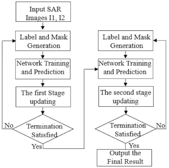
Figure 8.
Workflow of the two-stage updating strategy. The input SAR images are first generated to obtain initial label and mask at the pre-classification stage. Then, at the first updating stage, the network, as shown in Figure 6, learns iteratively to restore data diversity gradually. When at the second updating stage, the training process is similar to stage one, except for the updating function.
2.3.2. The Second Stage: Classifying in Uncertain Areas
The main purpose of this stage is to further classify pixels in uncertain areas. However, it can also classify some unlearned pixels in certain areas. The procedures are similar to that in stage one, except for the fusion mechanism. Unlike in stage one, if the values of and are 1 and 0.5, respectively, then the pixel can be labeled as a changed pixel.
At this stage, as the diversity of data is ensured through stage one, only two iterations are needed.
3. Results
This section first introduces the datasets that will be used in the experiment. Then, the evaluation criteria are introduced in detail. Next, several excellent change detection algorithms compared with the proposed method on the simulated datasets, and five real SAR datasets are presented. Finally, decomposition experiments are conducted to analyze the optimal parameters used in the final experiment.
3.1. Introduction of Datasets
The datasets contain simulated and real SAR images, which have been co-registered at the same place. To extensively conduct the experiments, one simulated dataset and five real SAR datasets are introduced.
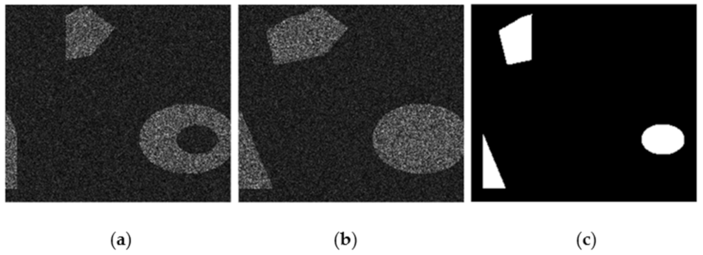
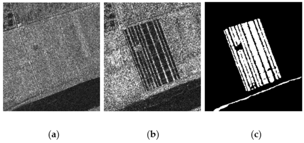
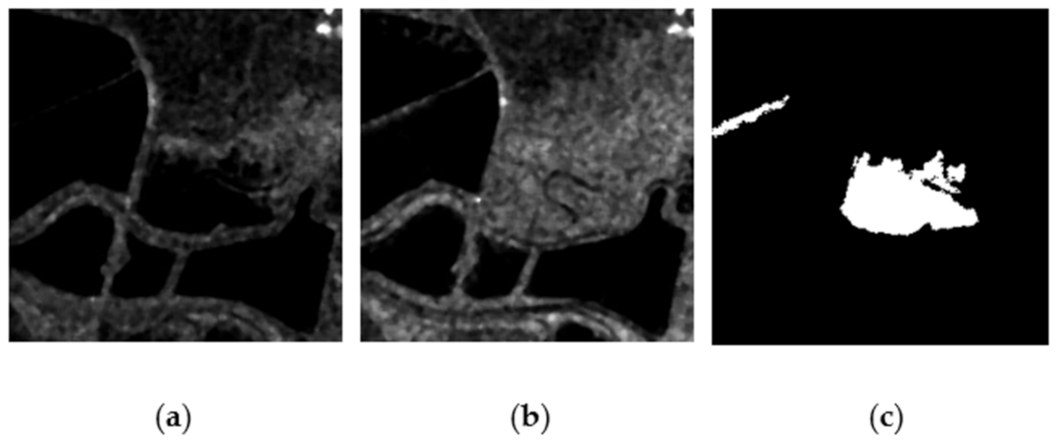
The simulated SAR images are created by adding multiplicative noise on two images with regularly changed areas, as shown in Figure 9. For real SAR images, the first dataset is the Ottawa dataset with a 10-m resolution, as shown in Figure 10. The images are provided by the National Defense Research and Development Canada. The two images are taken by the RADARSAT sensor in May and August 1997, respectively, and the size of the images in this paper is 290 × 350 pixels. The second and third datasets are cropped from the Yellow River dataset with a 3-m resolution, which was taken in June 2008 and June 2009, respectively. The Yellow River dataset was quite large; thus, we chose two representative regions, named Farmland C and Farmland D. The sizes of the above datasets are 306 × 291 and 257 × 289 pixels, as shown in Figure 11 and Figure 12. The fourth dataset is the San Francisco dataset with a 25-m resolution, which was captured in August 2003 and May 2004 with a size of 256 × 256 pixels, as shown in Figure 13. The fifth dataset is the Bern dataset with a 30-m resolution, which was captured in April and May 1999 with a size of 301 × 301, as shown in Figure 14.

Figure 9.
Simulated SAR images. (a,b) Simulated SAR images. (c) Ground truth image.
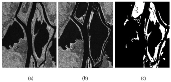
Figure 10.
Ottawa dataset with a 10-m resolution. (a) Image acquired in May 1997. (b) Image acquired in August 1997. (c) Ground truth.
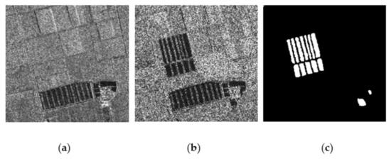
Figure 11.
Farmland C dataset with a 3-m resolution. (a) Image acquired in June 2008. (b) Image acquired in June 2009. (c) Ground truth.

Figure 12.
Farmland D dataset with a 3-m resolution. (a) Image acquired in June 2008. (b) Image acquired in June 2009. (c) Ground truth.

Figure 13.
San Francisco dataset with a 25-m resolution. (a) Image acquired in August 2003. (b) Image acquired in May 2004. (c) Ground truth.
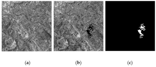
Figure 14.
Bern dataset with a 30-m resolution. (a) Image acquired in April 1999. (b) Image acquired in May 1999. (c) Ground truth.
3.2. Evaluation Criterion
The evaluation criteria are used to evaluate the accuracy of methods in different ways. Let FN represent the false-negative classified pixels, which means that changed pixels are undetected. FP represents the false-positive pixels, which means that unchanged pixels are wrongly classified. Both FN and FP are detection errors. Therefore, let OE represent the overall error and PCC represent the percentage correct classification, which can be expressed as follows:
where Nt represents the total of pixels in the result change map. The kappa [62] statistic is also widely used in the change detection task, because it contains more information. The formula for kappa is defined as
where Nc and Nu represent the total number of changed pixels and unchanged pixels in the ground truth map, respectively.
3.3. Experiment and Analysis
In this section, we chose several excellent algorithms—namely, DBN [39], NR-ELM [63], Gabor-PCANet [40], and CNN [33]—for comparison. Gabor-PCANet [40] is based on principal component analysis using two-stage convolution to achieve a good result. NR-ELM [63] uses an extreme learning machine to classify pixels. Reference [33] proposed a shallow CNN to classify pixels. In addition, references [39] and [63] needed to transform features into 1D shapes. References [40] and [33] preserved 2D spatial information by using convolutional operations. In this study, the parameters of the patch size, α, and w are set to 48, 0.5, and 3, respectively.
3.3.1. Results on Simulated Datasets
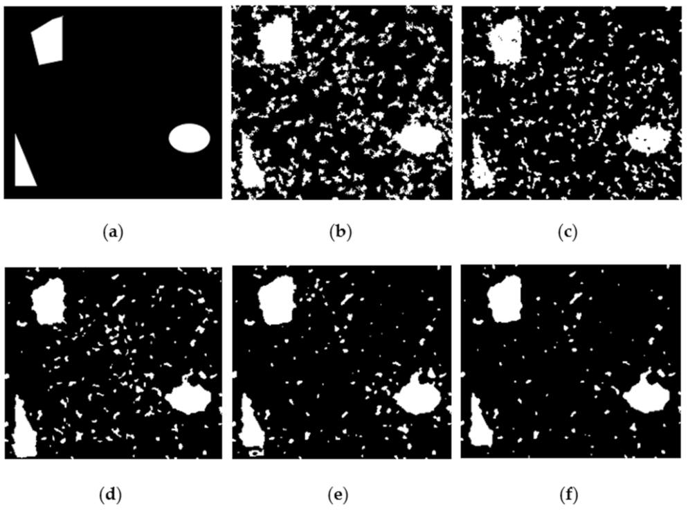
The change detection result on the simulated dataset is shown in Figure 15 and Table 2. As presented in Figure 15, both Gabor-PCANet [40] and NR-ELM [63] are seriously influenced by noise, which appears to have a high FP in Table 2. For PCANet, serious speckle noise occurs because of the strong density of noise in raw SAR images. When pre-classification is performed, too many noisy pixels are wrongly selected as labels. For NR-ELM [63],a neighborhood-based ratio operator is adopted to create labels. If the density of speckle noise is strong, then the value of the ratio could be large or small, which will lead to an inferior pre-classification result. Thus, as shown in Figure 15c, a lot of noise is scattered within the image. DBN utilizes stacked RBM to build a network with a strong learning ability. Thus, the visual result is much better compared with that of Gabor-PCANet [40] and NR-ELM [63]. However, it is still seriously influenced by noise. CNN [33] is more suitable for dealing with 2D images. However, because the sizes of patches are small, it cannot effectively learn the semantic information of the images. Thus, as shown in Figure 15e, many white spots exist in the change map.

Figure 15.
Change detection results on simulated SAR images. (a) Ground truth. (b) Result by Gabor-PCANet. (c) Result by NR-ELM. (d) Result by DBN. (e) Result by convolutional neural network (CNN). (f) Result by our proposed method.

Table 2.
Change detection result of the simulated synthetic aperture radar (SAR) dataset. CNN: convolutional neural network, FP: false-positives, FN: false-negatives, OE: overall error, and PCC: percentage correct classification.
The proposed method achieves the best results visually and numerically, as shown in Figure 15f and Table 2. Compared with PCANet, NR-ELM, and DBN, less noise is introduced by the proposed method. Compared with DBN [39] and CNN [33], the proposed method better preserves the shapes’ changed areas, as shown in Figure 15f. The above remarkable results were achieved because of two reasons. First, the design of iterative learning ensures the diversity of data and introduces less noise. Second, the designed CNN-based network not only preserves the spatial information well but can also exploit richer semantic information.
3.3.2. Results on the Ottawa Dataset
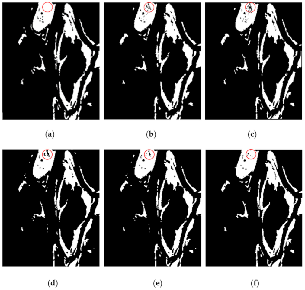
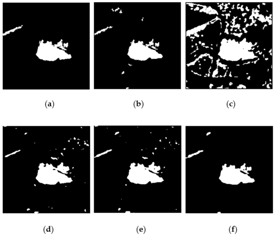
Figure 16 and Table 3 show the change detection result on the Ottawa dataset. The resolution of this dataset is a medium with 10 m. Moreover, the most changed areas are discriminative. Thus, as shown in Figure 16 and Table 3, all the methods achieved good results. As shown in Table 3, Gabor-PCANet [40] obtained the worst performance. Although little speckle noise was found in Figure 16b, the edges were blurred. NR-ELM [63] performed better than Gabor-PCANet [40]. The edges were sharp, and the details were better preserved. However, many false-negative pixels were produced. DBN [39] and CNN [33] had better learning ability than the above methods. Thus, as shown in Table 3, the results are competitive. However, the false-negative pixels for above two methods are still too high. All the above methods face the same problem in which the utilized pixels change dramatically to learn pixels that do not change noticeably. Thus, the FP and FN are unable to be balanced. As shown in red circles, when the change of backscattering is not obvious, all the above methods fail to effectively discriminate changed regions.
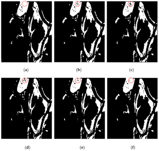
Figure 16.
Change detection results on the Ottawa dataset. (a) Ground truth. (b) Result by Gabor-PCANet. (c) Result by NR-ELM. (d) Result by DBN. (e) Result by CNN. (f) Result by our proposed method.

Table 3.
Change detection results of the Ottawa dataset.
The final change map obtained by our method contains little noise and preserves details well, as shown in Figure 16f. Our method has the lowest OE value among all the methods. Although the FP is higher than some previous methods, the FP and FN are balanced. Thus, the OE is the lowest, and the PCC is the best. As shown in the red circle, our proposed method obtains better visual results, because the data diversity is ensured by iterative learning.
3.3.3. Results on the San Francisco Dataset
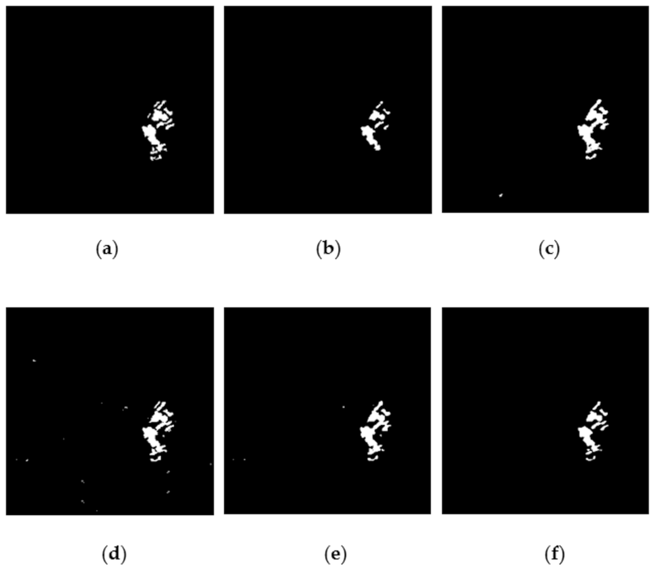
The results of the San Francisco dataset are shown in Figure 17 and Table 4. Similar to the Ottawa dataset, the changed area within two SAR images is discriminative. The resolution of this dataset is 25 m. As shown in Table 4, all methods except for NR-ELM [63] achieved good performance. The result obtained by NR-ELM [63] was seriously influenced by false alarms, and details of the changed area were poorly preserved, because too much noise was introduced during pre-classification. As shown in Figure 17b, Gabor-PCANet [40] performed much better. Few isolated white spots existed in the map. Compared with Gabor-PCANet [40], DBN [39] and CNN [33] contain more noise, resulting in a high FP, as shown in Table 4. The above two methods also face the problem of overlearning, such that the details of the changed area are not preserved well.
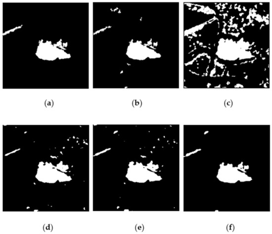
Figure 17.
Change detection results on the San Francisco dataset. (a) Ground truth. (b) Result by Gabor-PCANet. (c) Result by NR-ELM. (d) Result by DBN. (e) Result by CNN. (f) Result by our proposed method.

Table 4.
Change detection results of the San Francisco dataset.
Compared with the above methods, the change map obtained by our proposed method contains less noise and is very close to the ground truth reference, as shown in Figure 17f. As shown in Table 4, the proposed method obtains the best results quantitatively. The gap between FP and FN is the smallest, and balance is achieved.
3.3.4. Results on the Bern Dataset
The resolution of the dataset is 30 m. As the number of changed pixels in this dataset is small, all methods tend to obtain the change map with high accuracy. As shown in Figure 18 and Table 5, all methods suppress speckle noise well, because the change of backscattering is strong, such that discriminating changed areas is easy. Gabor-PCANet is the least satisfactory among all the methods, losing the details of the changed area. Compared with Gabor-PCANet, the edges of NR-ELM [63] are blurred. Both methods face the same problem of selecting unsuitable labels at the pre-classification stage. DBN [39] and CNN [33] perform better than these two methods, preserving the details of changed areas better, yet some white spots are produced, as shown in Figure 18d,e.
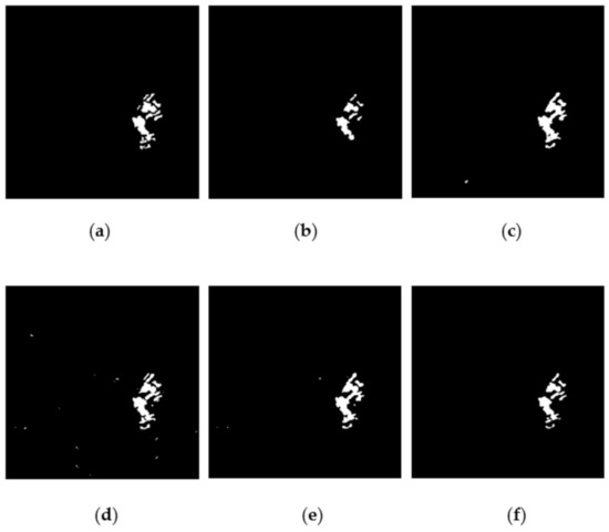
Figure 18.
Change detection results on the Bern dataset. (a) Ground truth. (b) Result by Gabor-PCANet. (c) Result by NR-ELM. (d) Result by DBN. (e) Result by CNN. (f) Result by our proposed method.

Table 5.
Change detection results of the Bern dataset.
As shown in Figure 18f, the change map obtained by our proposed method is very close to the ground truth reference. Compared with the above methods, our change map contains less noise and restores the changed area well. As shown in Table 5, although the kappa value of our method is slightly inferior to that of DBN [39], our method gains the highest PCC value.
3.3.5. Results on the Farmland C Dataset
The results of the Farmland C dataset are shown in Figure 19 and Table 6. The resolution of the dataset is 3 m, which is much higher than that of the above datasets. NR-ELM [63] obtains the worst result both for the visual and PCC values. For the visual result, the changed area is incomplete. For the numerical value, the FN is the highest, because too many changed pixels are abandoned at the pre-classification stage. As shown in Figure 19d, DBN [39] restores changed areas better. However, many white spots are produced, resulting in a large FP value, as shown in Table 6, because DBN has a better learning ability than NR-ELM, and more noisy pixels are introduced when creating a label. The resolution of the dataset is much higher, which is why richer texture information can help extract more discriminative features. Gabor-PCANet [40] and CNN [33] are more suitable for dealing with high-resolution SAR images, because they are based on the convolutional operation. As shown in Figure 19b, Gabor-PCANet has the least noise and is very close to the ground truth reference, because a suitable label is selected at the pre-classification stage. The performance of CNN [33] is also competitive. However, some isolated white spots are produced.
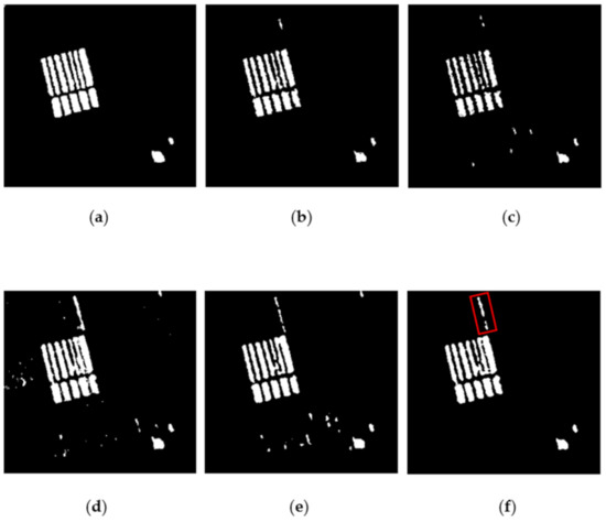
Figure 19.
Change detection results on the Farmland C dataset. (a) Ground truth. (b) Result by Gabor-PCANet. (c) Result by NR-ELM. (d) Result by DBN. (e) Result by CNN. (f) Result by our proposed method.

Table 6.
Change detection results of the Farmland C dataset.
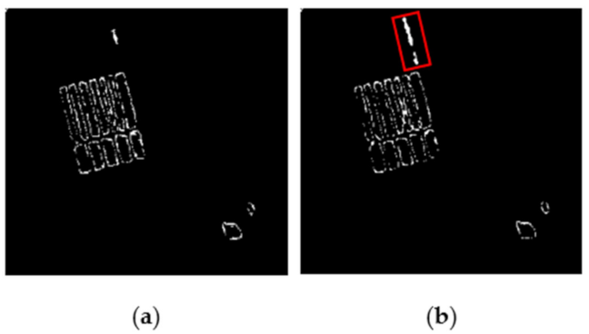
The change map of our method is very close to that of Gabor-PCANet. As shown in Figure 20, for the change map of our proposed method, fewer wrongly classified pixels exist at the edges of changed areas. However, more false-positive pixels are produced within the red rectangle. When comparing two bitemporal SAR images, we find that the noise is caused by the changing of two neighboring farmlands and not by speckle noise. Thus, all the above methods recognize the changed pixels in the red rectangle as truly changed pixels. Finally, as shown in Table 6, our proposed method obtains the highest PCC and kappa values.

Figure 20.
Wrongly classified pixels in the final change map. (a) Error pixels for Gabor-PCANet. (b) Error for our proposed method.
3.3.6. Results on the Farmland D Dataset
The resolution of Farmland D dataset is also 3 m. The shape of changed areas looks like strips. Thus, restoring changed areas is more difficult. Figure 21 and Table 7 present the final change detection results on this dataset. NR-ELM [63] and DBN [39] obtain worse performances, because they missed many changed areas. These results occurred because too many changed pixels are abandoned at the pre-classification stage. Moreover, the above two methods transform images into 1D features, which also lose spatial information. Gabor-PCANet [40] and CNN [33] have better visual and numerical results than NR-ELM [63] and DBN [39], because they can fully utilize the rich spatial and texture information of the images. However, more noisy spots are produced for CNN [33], and the changed areas are overlearned.
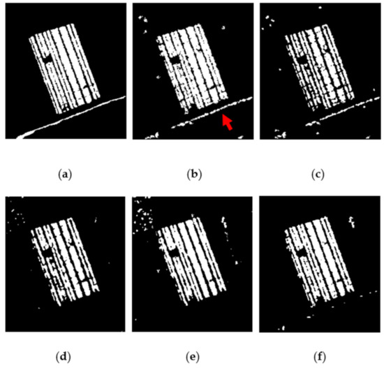
Figure 21.
Change detection results on the Farmland D dataset. (a) Ground truth. (b) Result by Gabor-PCANet. (c) Result by NR-ELM. (d) Result by DBN. (e) Result by CNN. (f) Result by our proposed method.

Table 7.
Change detection results of the Farmland D dataset
Gabor-PCANet [40] seems to obtain better visual results than our method at the position of the red arrow. However, as shown in Figure 22, most pixels at the position of the red arrow for Gabor-PCANet are false-positives. Gabor-PCANet also contains more wrong pixels at the edges of the changed areas. Thus, the visual results of our method are better. As shown in Table 7, our proposed method also obtains the best results quantitatively. This performance was achieved because of two reasons. First, our network can extract more semantic and spatial information to create more discriminative features. Second, two-stage learning ensures the diversity of data and introduces less noise.
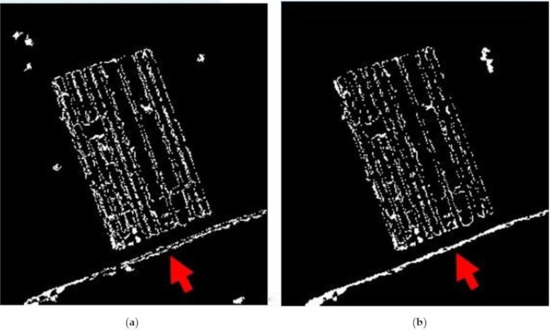
Figure 22.
Wrongly classified pixels in the final change map. (a) Error pixels for Gabor-PCANet. (b) Errors for our proposed method.
3.4. Parameter Analysis
In this section, three main factors are discussed: (a) patch sizes of the input images, (b) mean filter threshold (α), and (c) window size of the mean filter (w). When selecting patch sizes, larger patches tend to be less time-consuming. However, it results in fewer training samples, which may lead to overfitting. α and w are the key factors in eliminating speckle noise in the newly learned change map.
3.4.1. Analysis of the Patch Size
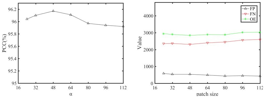
Given that the network is deep and contains several max pooling operations, the input patch should have a minimum size of 16 × 16 pixels. In this study, we conduct experiments using patches with sizes of 24 × 24, 32 × 32, 48 × 48, 64 × 64, 80 × 80, 96 × 96, and 112 × 112 pixels. Given that the Farmland D dataset is popularly used in many articles and the dataset is more difficult, we use this dataset to conduct our experiments. The results are illustrated in Figure 23. When the sizes of the patches are 24 to 64, the results are very close. However, as the sizes of patches increase, the accuracy drops by about 0.2%. This decrease may be caused by the decrease in the training samples. To save computational time, patches with sizes of 24 and 32 are not considered. Patches with sizes of 48 and 64 obtain similar results. In this paper, a patch with 48 × 48 pixels was selected, because it obtained the highest accuracy. A patch with 64 × 64 pixels can also be selected if computational time is the first priority.
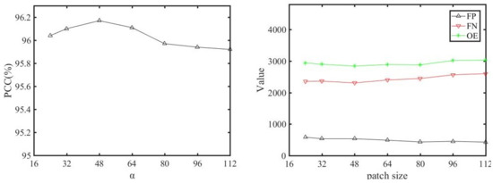
Figure 23.
The influence of the patch size evaluated on the Farmland D dataset.
3.4.2. Analysis of the Filter Threshold (α)
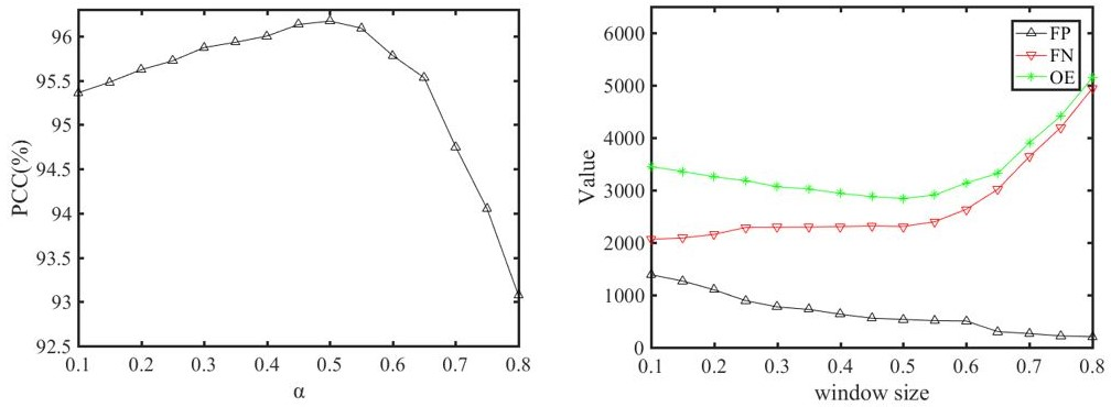
In this part, the impact of α is discussed through an experiment on the Farmland D dataset. As introduced before, the value of α at the pre-classification stage is set to 0.7. However, this value does not need to be 0.7 at the updating stage, because the noise in the newly learned change map is greatly eliminated. In this experiment, the values of α are set to 0.1, 0.15, 0.2, 0.25, 0.3, 0.35, 0.4, 0.45, 0.5, 0.55, 0.6, 0.65, 0.7, 0.75, and 0.8. As shown in Figure 24, an excessively large α will lead to a poor performance, because the newly learned pixels are eliminated by the filtering process. Therefore, with the increase in α, the FP decreases and FN increases. When α is small, the results are better, because most of the newly learned pixels are correct, such that a smaller α can satisfy the performance. When the value of α is 0.5, the performance is better. In this paper, we set α as 0.5 when updating.

Figure 24.
The influence of α evaluated on the Farmland D dataset.
3.4.3. Analysis of the Window Size of the Filter (w)
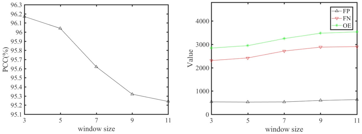
The window size of the filter also influences the effectiveness of noise suppression. This study conducts five experiments using five different window sizes on the Farmland D dataset to verify the impact of this factor. The sizes are set to 3 × 3, 5 × 5, 7 × 7, 9 × 9, and 11 × 11. As shown in Figure 25, the accuracy decreases as the window size increases, because little noise exists in the newly generated change map. Thus, a larger filter window and α do not need to be used. When the window size is larger, the map tends to be smoother, resulting in higher FP and FN values. When the window size is 3 × 3, the result is optimal.
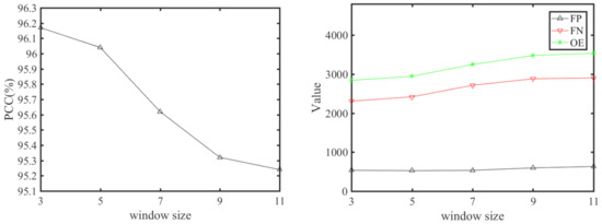
Figure 25.
The influence of w (Window Size of the Filter) evaluated on the Farmland D dataset.
3.5. Ablation Analysis
3.5.1. Analysis of Network
This section will discuss the effectiveness of the multilayer fusion network and the two-stage label updating mechanism. First, without the multilayer fusion function in the network, the features F1, F2, and F3 in Equation (8) will be ignored. The final feature is no longer fused and is described as follows:
Then, the three conditions are compared to verify the effectiveness of the updating strategy: (1) without updating and (2) with only a one-stage updating strategy. Equation (11) instead of (10) is utilized to refine the newly generated change maps. Only the second stage is remains. The other condition is (3) the two-stage updating strategy. Extensive experiments are conducted, as shown in Table 8.

Table 8.
Analysis of the network and updating function.
3.5.2. Analysis of the Computational Time
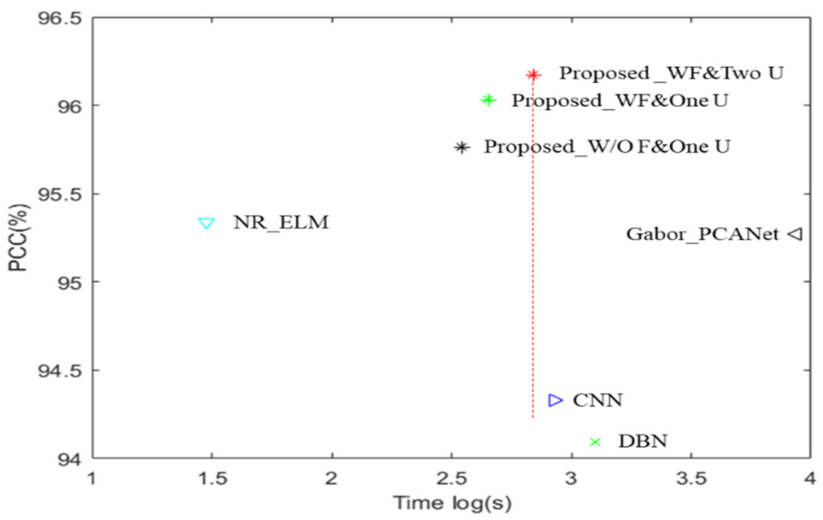
In this section, the computational time of the proposed method will be discussed. As shown in Figure 26, our proposed method achieves a better computational cost performance, because our model learns and outputs data in the form of large patches, which accelerates the computational process. Compared with NR-ELM, our model costs more time but is far more accurate. Compared with CNN [33], Gabor-PCANet [40], and DBN [39], our method obtains better results and costs less time. The paper also makes a contrast to the method itself. If the network has no fusion process, then the computational time is greatly reduced, and the accuracy is still better than that of the above methods. In the case with fusion function, the accuracy is improved, and the computational time is increased. A trade-off exists between the network complexity and computing time.
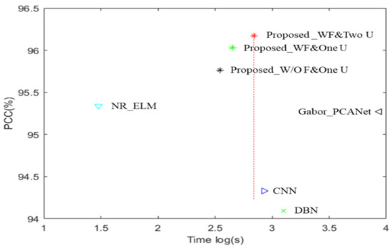
Figure 26.
Comparison of the computational time and accuracy.
4. Conclusions
In this paper, a multilayer fusion network with an updating strategy is proposed. Different existing AI-based methods in the field of change the detection of SAR images, the method is patch-based and unsupervised, and can learn and classify patches in an end-to-end way. In addition, a two-stage updating strategy is designed to let the network learn iteratively. The first stage of learning greatly restores the diversity of data within certain areas, and the second stage of learning fully classifies pixels within uncertain areas into changed or unchanged pixels. Several advantages exist compared with the existing methods. First, the proposed network is based on CNN, which can fully exploit the semantic and spatial information of SAR images. Second, the method is based on patches instead of pixels, thereby greatly reducing the computational cost and enlarging the receptive field of the network. Third, the designed method is unsupervised and can learn patches in an end-to-end way. By introducing the mask function and two-stage updating strategy, training labels are selected by the network itself. Changed areas are restored gradually, and less noise is introduced at the same time. Thus, more details can be preserved, and less noise is introduced in the results maps. The experimental results illustrate that our proposed method can obtain better results both visually and quantitatively. In the future, our attention will be paid to the coefficient α. In this paper, the value of α is constant at the updating stage. If the value of α can change automatically according to the dataset and loss value, then the performance of the network could improve.
Author Contributions
Methodology, Y.S.; validation, Y.S.; writing—original draft preparation, Y.S.; writing—review and editing, Y.S., W.L. and M.Y.; supervision, S.H. and W.L.; suggestions, P.C.; All authors have read and agreed to the published version of the manuscript.
Funding
This work was supported in part by the Sichuan Science and Technology Program under Grants 2020YFG0134, 2018JY0602, and 2018GZDX0024, in part by the funding from Sichuan University under Grant 2020SCUNG205 (corresponding author: W.L.).
Data Availability Statement
Not Applicable.
Conflicts of Interest
The authors declare no conflict of interest.
References
- Quan, S.; Xiong, B.; Xiang, D.; Zhao, L.; Zhang, S.; Kuang, G. Eigenvalue-based urban area extraction using polarimetric SAR data. IEEE J. Sel. Top. Appl. Earth Observ. Remote Sens. 2018, 11, 458–471. [Google Scholar] [CrossRef]
- Azzouzi, S.A.; Vidal-Pantaleoni, A.; Bentounes, H.A. Desertification monitoring in Biskra, algeria, with Landsat imagery by means of supervised classification and change detection methods. IEEE Access 2017, 5, 9065–9072. [Google Scholar] [CrossRef]
- Barreto, T.L.; Rosa, R.A.; Wimmer, C.; Nogueira, J.B.; Almeida, J.; Cappabianco, F.A.M. Deforestation change detection using high-resolution multi-temporal X-Band SAR images and supervised learning classification. In Proceedings of the IEEE International Geoscience and Remote Sensing Symposium (IGARSS), Beijing, China, 10–15 July 2016; pp. 5201–5204. [Google Scholar]
- Song, D.; Tan, X.; Wang, B.; Zhang, L.; Shan, X.; Cui, J. Integration of super-pixel segmentation and deep-learning methods for evaluating earthquake-damaged buildings using single-phase remote sensing imagery. Int. J. Remote Sens. 2020, 41, 1040–1066. [Google Scholar] [CrossRef]
- Brisco, B.; Schmitt, A.; Murnaghan, K.; Kaya, S.; Roth, A. SAR polarimetric change detection for flooded vegetation. Int. J. Digit. Earth 2013, 6, 103–114. [Google Scholar] [CrossRef]
- Hussain, M.; Chen, D.; Cheng, A.; Wei, H.; Stanley, D. Change detection from remotely sensed images: From pixel-based to object- based approaches. ISPRS J. Photogramm. Remote Sens. 2013, 80, 91–106. [Google Scholar] [CrossRef]
- Coppin, P.R.; Bauer, M.E. Digital change detection in forest ecosystems with remote sensing imagery. Remote Sens. Rev. 1996, 13, 207–234. [Google Scholar] [CrossRef]
- Rignot, E.J.; Van Zyl, J.J. Change detection techniques for ERS-1 SAR data. IEEE Trans. Geosci. Remote Sens. 1993, 31, 896–906. [Google Scholar] [CrossRef]
- Chen, J.; Gong, P.; He, C.; Pu, R.; Shi, P. Land-use/land-cover change detection using improved change-vector analysis. Photogramm. Eng. Remote Sens. 2003, 69, 369–379. [Google Scholar] [CrossRef]
- Nackaerts, K.; Vaesen, K.; Muys, B.; Coppin, P. Comparative performance of a modified change vector analysis in forest change detection. Int. J. Remote Sens. 2005, 26, 839–852. [Google Scholar] [CrossRef]
- Ji, W.; Ma, J.; Twibell, R.W.; Underhill, K. Characterizing urban sprawl using multi-stage remote sensing images and landscape metrics. Comput. Environ. Urban Syst. 2006, 30, 861–879. [Google Scholar] [CrossRef]
- Lunetta, R.S.; Knight, J.F.; Ediriwickrema, J.; Lyon, J.G.; Worthy, L.D. Land-cover change detection using multi-temporal MODIS NDVI data. Remote Sens. Environ. 2006, 105, 142–154. [Google Scholar] [CrossRef]
- Bovolo, F.; Bruzzone, L. A detail-preserving scale-driven approach to change detection in multitemporal SAR images. IEEE Trans. Geosci. Remote Sens. 2005, 43, 2963–2972. [Google Scholar] [CrossRef]
- Inglada, J.; Mercier, G. A new statistical similarity measure for change detection in multitemporal SAR images and its extension to multiscale change analysis. IEEE Trans. Geosci. Remote Sens. 2007, 45, 1432–1445. [Google Scholar] [CrossRef]
- Hou, B.; Wei, Q.; Zheng, Y.; Wang, S. Unsupervised change detection in SAR image based on Gauss-log ratio image fusion and compressed projection. IEEE J. Sel. Top. Appl. Earth Obs. Remote Sens. 2014, 7, 3297–3317. [Google Scholar] [CrossRef]
- Gong, M.; Cao, Y.; Wu, Q. A neighborhood-based ratio approach for change detection in SAR images. IEEE Geosci. Remote Sens. Lett. 2012, 9, 307–311. [Google Scholar] [CrossRef]
- Kittler, J.; Illingworth, J. Minimum error thresholding. Pattern Recognit. 1986, 19, 41–47. [Google Scholar] [CrossRef]
- Figueiredo, M.A.; Nowak, R.D. An EM algorithm for wavelet-based image restoration. IEEE Trans. Image Process. 2003, 12, 906–916. [Google Scholar] [CrossRef]
- Dunn, J.C. A fuzzy relative of the ISODATA process and its use in detecting compact well-separated clusters. J. Cybern. 1973, 3, 32–57. [Google Scholar] [CrossRef]
- Krinidis, S.; Chatzis, V. A robust fuzzy local information C-means clustering algorithm. IEEE Trans. Image Process. 2010, 19, 1328–1337. [Google Scholar] [CrossRef]
- Gong, M.; Zhou, Z.; Ma, J. Change detection in synthetic aperture radar images based on image fusion and fuzzy clustering. IEEE Trans. Image Process. 2012, 21, 2141–2151. [Google Scholar] [CrossRef]
- Wang, F.; Wu, Y.; Zhang, Q.; Zhang, P.; Li, M.; Lu, Y. Unsupervised change detection on SAR images using triplet Markov field model. IEEE Geosci. Remote Sens. Lett. 2012, 10, 697–701. [Google Scholar] [CrossRef]
- Marin, C.; Bovolo, F.; Bruzzone, L. Building change detection in multitemporal very high resolution SAR images. IEEE Trans. Geosci. Remote Sens. 2014, 53, 2664–2682. [Google Scholar] [CrossRef]
- Lefebvre, A.; Corpetti, T.; Hubert-Moy, L. Object-oriented approach and texture analysis for change detection in very high resolution images. In Proceedings of the IGARSS 2008—2008 IEEE International Geoscience and Remote Sensing Symposium, Boston, MA, USA, 7–11 July 2008; Volume 4. p. IV–663. [Google Scholar]
- Liu, B.; Hu, H.; Wang, H.; Wang, K.; Liu, X.; Yu, W. Superpixel-based classification with an adaptive number of classes for polarimetric SAR images. IEEE Trans. Geosci. Remote Sens. 2012, 51, 907–924. [Google Scholar] [CrossRef]
- Wu, Z.; Hu, Z.; Fan, Q. Superpixel-based unsupervised change detection using multi-dimensional change vector analysis and SVM-based classification. ISPRS Ann. Photogramm. Remote Sens. Spat. Inf. Sci. 2012, 7, 257–262. [Google Scholar] [CrossRef]
- Barreto, T.L.; Rosa, R.A.; Wimmer, C.; Moreira, J.R.; Bins, L.S.; Cappabianco, F.A.M.; Almeida, J. Classification of Detected Changes from Multitemporal High-Res Xband SAR Images Intensity and Texture Descriptors from SuperPixels. IEEE J. Sel. Top. Appl. Earth Observ. 2016, 9, 5436–5448. [Google Scholar] [CrossRef]
- Chen, G.; Hay, G.J.; Carvalho, L.M.; Wulder, M.A. Object-based change detection. Int. J. Remote Sens. 2012, 33, 4434–4457. [Google Scholar] [CrossRef]
- Daudt, R.C.; Le Saux, B.; Boulch, A.; Gousseau, Y. Urban Change Detection for Multispectral Earth Observation Using Convolutional Neural Networks. In Proceedings of the IEEE International Geoscience and Remote Sensing Symposium, Valencia, Spain, 22–27 July 2018; pp. 2115–2118. [Google Scholar]
- Yang, K.; Xia, G.S.; Liu, Z.; Du, B.; Yang, W.; Pelillo, M. Asymmetric Siamese Networks for Semantic Change Detection. arXiv 2020, arXiv:2010.05687. [Google Scholar]
- Peng, D.; Bruzzone, L.; Zhang, Y.; Guan, H.; Ding, H.; Huang, X. SemiCDNet: A Semisupervised Convolutional Neural Network for Change Detection in High Resolution Remote-Sensing Images. IEEE Trans. Geosci. Remote Sens. 2020. [Google Scholar] [CrossRef]
- Yang, M.; Jiao, L.; Liu, F.; Hou, B.; Yang, S. Transferred Deep Learning-Based Change Detection in Remote Sensing Images. IEEE Trans. Geosci. Remote Sens. 2019, 57, 6960–6973. [Google Scholar] [CrossRef]
- Li, Y.; Peng, C.; Chen, Y.; Jiao, L.; Zhou, L. A deep learning method for change detection in synthetic aperture radar images. IEEE Trans. Geosci. Remote Sens. 2019, 57, 5751–5763. [Google Scholar] [CrossRef]
- Liu, J.; Gong, M.; Qin, K.; Zhang, P. A deep convolutional coupling network for change detection based on heterogeneous optical and radar images. IEEE Trans. Neural Netw. Learn. Syst. 2016, 29, 545–559. [Google Scholar] [CrossRef] [PubMed]
- Geng, J.; Ma, X.; Zhou, X.; Wang, H. Saliency-Guided Deep Neural Networks for SAR Image Change Detection. IEEE Trans. Geosci. Remote Sens. 2019, 57, 7365–7377. [Google Scholar] [CrossRef]
- Du, B.; Ru, L.; Wu, C.; Zhang, L. Unsupervised deep slow feature analysis for change detection in multi-temporal remote sensing images. IEEE Trans. Geosci. Remote Sens. 2019, 57, 9976–9992. [Google Scholar] [CrossRef]
- Planinšič, P.; Gleich, D. Temporal change detection in SAR images using log cumulants and stacked autoencoder. IEEE Geosci. Remote Sens. Lett. 2018, 15, 297–301. [Google Scholar] [CrossRef]
- Gong, M.; Zhan, T.; Zhang, P.; Miao, Q. Superpixel-Based Difference Representation Learning for Change Detection in Multispectral Remote Sensing Images. IEEE Trans. Geosci. Remote Sens. 2017, 55, 2658–2673. [Google Scholar] [CrossRef]
- Gong, M.; Zhao, J.; Liu, J.; Miao, Q.; Jiao, L. Change detection in synthetic aperture radar images based on deep neural networks. IEEE Trans. Neural Netw. Learn. Syst. 2016, 27, 125–138. [Google Scholar] [CrossRef] [PubMed]
- Gao, F.; Dong, J.; Li, B.; Xu, Q. Automatic change detection in synthetic aperture radar images based on PCANet. IEEE Geosci. Remote Sens. Lett. 2016, 13, 1792–1796. [Google Scholar] [CrossRef]
- Gao, Y.; Gao, F.; Dong, J.; Wang, S. Change Detection from Synthetic Aperture Radar Images Based on Channel Weighting-Based Deep Cascade Network. IEEE J. Sel. Top. Appl. Earth Observ. 2019, 12, 4517–4529. [Google Scholar] [CrossRef]
- Gong, M.; Yang, H.; Zhang, P. Feature learning and change feature classification based on deep learning for ternary change detection in SAR images. ISPRS J. Photogramm. Remote Sens. 2017, 129, 212–225. [Google Scholar] [CrossRef]
- Lei, Y.; Liu, X.; Shi, J.; Lei, C.; Wang, J. Multiscale superpixel segmentation with deep features for change detection. IEEE Access 2019, 7, 36600–36616. [Google Scholar] [CrossRef]
- Lv, N.; Chen, C.; Qiu, T.; Sangaiah, A.K. Deep learning and superpixel feature extraction based on contractive autoencoder for change detection in SAR images. IEEE Trans. Ind. Inf. 2018, 14, 5530–5538. [Google Scholar] [CrossRef]
- El Amin, A.M.; Liu, Q.; Wang, Y. Zoom out cnns features for optical remote sensing change detection. In Proceedings of the 2017 2nd International Conference on Image, Vision and Computing (ICIVC), Chengdu, China, 2–4 June 2017; pp. 812–817. [Google Scholar]
- Zhang, X.; Liu, G.; Zhang, C.; Atkinson, P.M.; Tan, X.; Jian, X.; Zhou, X.; Li, Y. Two-phase object-based deep learning for multi-temporal SAR image change detection. Remote Sens. 2020, 12, 548. [Google Scholar] [CrossRef]
- Chen, J.; Liu, H.; Hou, J.; Yang, M.; Deng, M. Improving Building Change Detection in VHR Remote Sensing Imagery by Combining Coarse Location and Co-Segmentation. ISPRS Int. J. Geo-Inf. 2018, 7, 213. [Google Scholar] [CrossRef]
- Chen, H.; Shi, Z. A Spatial-Temporal Attention-Based Method and a New Dataset for Remote Sensing Image Change Detection. Remote Sens. 2020, 12, 1662. [Google Scholar] [CrossRef]
- Hou, B.; Wang, Y.; Liu, Q. Change detection based on deep features and low rank. IEEE Geosci. Remote Sens. Lett. 2017, 14, 2418–2422. [Google Scholar] [CrossRef]
- Zhan, Y.; Fu, K.; Yan, M.; Sun, X.; Wang, H.; Qiu, X. Change detection based on deep siamese convolutional network for optical aerial images. IEEE Geosci. Remote Sens. Lett. 2017, 14, 1845–1849. [Google Scholar] [CrossRef]
- Daudt, R.C.; Le Saux, B.; Boulch, A. Fully convolutional siamese networks for change detection. In Proceedings of the ICIP, Athens, Greece, 7–10 October 2018; pp. 4063–4067. [Google Scholar]
- Guo, E.; Fu, X.; Zhu, J.; Deng, M.; Liu, Y.; Zhu, Q.; Li, H. Learning to measure change: Fully convolutional siamese metric networks for scene change detection. arXiv 2018, arXiv:1810.09111. [Google Scholar]
- Chen, J.; Yuan, Z.; Peng, J.; Chen, L.; Huang, H.; Zhu, J.; Liu, Y.; Li, H. DASNet: Dual attentive fully convolutional Siamese networks for change detection of high resolution satellite images. arXiv 2020, arXiv:2020:2003.03608. [Google Scholar] [CrossRef]
- Zhang, P.; Gong, M.; Zhang, H.; Liu, J.; Ban, Y. Unsupervised Difference Representation Learning for Detecting Multiple Types of Changes in Multitemporal Remote Sensing Images. IEEE Trans. Geosci. Remote Sens. 2018, 57, 2277–2289. [Google Scholar] [CrossRef]
- Gao, Y.; Gao, F.; Dong, J.; Wang, S. Transferred deep learning for sea ice change detection from synthetic-aperture radar images. IEEE Geosci. Remote Sens. Lett. 2019, 16, 1655–1659. [Google Scholar] [CrossRef]
- Peng, D.; Zhang, Y.; Guan, H. End-to-end change detection for high resolution satellite images using improved unet++. Remote Sens. 2019, 11, 1382. [Google Scholar] [CrossRef]
- Ji, S.; Wei, S.; Lu, M. Fully Convolutional Networks for Multisource Building Extraction from an Open Aerial and Satellite Imagery Data Set. IEEE Trans. Geosci. Remote Sens. 2018, 57, 574–586. [Google Scholar] [CrossRef]
- Qiu, Y.; Wang, R.; Tao, D.; Cheng, J. Embedded block residual network: A recursive restoration model for single-image super-resolution. In Proceedings of the ICCV, Seoul, Korea, 27 October–2 November 2019; pp. 4180–4189. [Google Scholar]
- Ronneberger, O.; Fischer, P.; Brox, T. U-net: Convolutional networks for biomedical image segmentation. In Proceedings of the MICCAI, Munich, Germany, 5–9 October 2015; pp. 234–241. [Google Scholar]
- Zhan, T.; Gong, M.; Liu, J.; Zhang, P. Iterative feature mapping network for detecting multiple changes in multi-source remote sensing images. ISPRS J. Photogramm. Remote Sens. 2018, 146, 38–51. [Google Scholar] [CrossRef]
- Hur, J.; Roth, S. Iterative residual refinement for joint optical flow and occlusion estimation. In Proceedings of the CVPR, Long Beach, CA, USA, 16–20 June 2019; pp. 5754–5763. [Google Scholar]
- Rosenfield, G.H.; Fitzpatrick-Lins, K. A coefficient of agreement as a measure of thematic classification accuracy. Photogram. Eng. Remote Sens. 1986, 52, 223–227. [Google Scholar]
- Gao, F.; Dong, J.; Li, B.; Xu, Q.; Xie, C. Change detection from synthetic aperture radar images based on neighborhood-based ratio and extreme learning machine. J. Appl. Remote Sens. 2016, 10, 046019. [Google Scholar] [CrossRef]
Publisher’s Note: MDPI stays neutral with regard to jurisdictional claims in published maps and institutional affiliations. |
© 2021 by the authors. Licensee MDPI, Basel, Switzerland. This article is an open access article distributed under the terms and conditions of the Creative Commons Attribution (CC BY) license (http://creativecommons.org/licenses/by/4.0/).


