Article

Spatiotemporal Heterogeneity Analysis of Yangtze River Delta Urban Agglomeration: Evidence from Nighttime Light Data (2001–2019)

1
Aerospace Information Research Institute, Chinese Academy of Sciences, Beijing 100101, China
2
University of Chinese Academy of Science, Beijing 100049, China
3
Max Planck Institute for Meteorology, 20146 Hamburg, Germany
4
Department of Geosciences and Natural Resource Management, University of Copenhagen, DK-1350 Copenhagen, Denmark
*
Author to whom correspondence should be addressed.
Remote Sens. 2021, 13(7), 1235; https://doi.org/10.3390/rs13071235
Submission received: 23 January 2021 / Revised: 15 March 2021 / Accepted: 19 March 2021 / Published: 24 March 2021

Abstract

:
The long-term changes of the relationship between nighttime light and urbanization related built-up areas are explored using nighttime light data obtained from the Defense Meteorological Satellite Program/Operational Linescan System (DMSP/OLS, data before 2013) and the Suomi National Polar-orbiting Partnership Visible Infrared Imaging Radiometer Suite (NPP/VIIRS, data after 2012) and information of the spatiotemporal heterogeneity of urban evolution. This study assimilates two datasets and diagnoses the spatial heterogeneity in administrative city scale based on built-up area tendencies, temporal heterogeneity in pixel scale based on nighttime light intensity tendencies, and GDP associated spatiotemporal variability over the Yangtze River Delta comparing the first two decades of this century (2001–2010 versus 2011–2019). The analysis reveals the following main results: (1) The built-up areas have generally increased in the second period with the center of fast expansion moving southward, including Suzhou-Wuxi-Changzhou, Hangzhou, Ningbo, Nanjing, and Hefei. (2) Urban development in the original city core has saturated and is spilling over to the suburbs and countryside, leading to nighttime light intensity tendency shift from a “rapid to moderate” and a “moderate to rapid” development (a “hot to cold” and a “cold to hot” spatial clustering distribution). (3) The tendency shifts of built-up area and nighttime light intensity occur most frequently in 2010, after which the urban development is transforming from light intensity growth to built-up area growth, particularly in the developed city cores. The urban agglomeration process with nighttime light intensity reaching saturation prior to the urban development spreading into the surrounding suburbs and countryside, appears to be a suitable model, which provides insights in addressing related environmental problems and contribute to regional sustainable urban planning and management.

Graphical Abstract

1. Introduction

Urban agglomeration is a highly developed spatial form of integrated cities, which can be defined as a contiguously built-up area, shaped by one core city or by several adjacent cities, sharing industry-, infrastructure-, and housing-land use with high-density levels with embedded open spaces [1,2,3]. It has been witnessed worldwide in recent decades as one of the most significant changes in human society, and as a “dynamic, multidimensional socio-spatial process” [4]. Until now, 55% of the world’s population lives in the urban areas, and it is predicted that this number will reach 68% by 2050 [5]. Although urban agglomeration has stimulated rapid economic growth, this process has brought many environmental problems, including green space occupation, water scarcity, water and air pollution, and the urban heat island effects, particularly for developing countries [6,7,8,9,10].
China has been experiencing intensive urbanization since the 1980s, spatial forms of integrated cities are also noticed, for example, the Beijing–Tianjin–Hebei (BTH), the Yangtze River Delta (YRD), and the Pearl River Delta (PRD) regions [11,12,13,14,15]. Spatial and temporal heterogeneities of urbanization were first noticed by the Chinese population geographer Hu Huanyong in 1935 who proposed the “geo-demographic demarcation line” [16] separating the eastern and western parts of the country. The eastern part covers 36% of China, but accounts for 96% of the Chinese population. After 2000, the population in the west grew faster than in the east, but the growth did not change the situation. Urbanization shares a similar geographical distribution as population showing a fast development in the eastern and a slow development in the western regions [17,18].
Understanding the spatiotemporal dynamics of the urban agglomeration is crucial to optimize urban land use patterns, to support regional urban development strategies, and thus to address environmental problems related to fast changes in urban land cover [19]. Nighttime light from the Suomi National Polar orbiting Partnership visible infrared imaging radiometer suite (NPP/VIIRS) offers a new data source for extracting urban information. Efforts have been made to rapidly extract relatively accurate urban areas such as built-up [20] or impervious surface areas [21], and to reveal the responses of nighttime light intensity to socioeconomic development, for example, urban land expansion [22], human population [23], electric power consumption [24], gross domestic product and other socioeconomic variables [25,26,27].
The reported nighttime light based spatiotemporal heterogeneity of urban agglomeration in China is analyzed using data either from a single satellite [28] or from assimilation of more than one satellite [29,30,31]. It considers spatiotemporal heterogeneity by comparing (1) the three major urban agglomeration: Beijing–Tianjin–Hebei, Yangtze River Delta and Pearl River Delta [11,32]; (2) cities from eastern coastal region with cities from western mountainous region [33,34]; and (3) city core with the surrounding suburbs [35]. In applications, NPP/VIIRS nighttime light data are of much better quality than the nighttime light data from the Defense Meteorological Satellite Program Operational Linescan System (DMSP/OLS), but these two datasets suffer from the drawbacks of blooming effects from the near-infrared band [23,36,37]. Furthermore, DMSP/OLS images are inherently blurred, due to the footprint expanding away from the nadir, the limited data storage and the geo-location errors [38].
In summarizing, combined with nighttime light from the DMSP/OLS and NPP/VIIRS, 20 years of nighttime light data are provided as a response to the increasing demand for analyzing the effects of the changes of built-up areas. However, to our knowledge, few studies have been concerned with the data assimilation procedures associated with a time changing threshold to identify the built-up areas from DMSP/OLS (data before 2013) and NPP/VIIRS (data after 2012), although this is necessary due to considerable inconsistencies, different spatiotemporal quality, drawbacks of blooming effects and radiometric heterogeneities; in this paper, a time changing threshold is introduced to identify the built-up areas. Thus, to obtain a consistent analysis, it is urgently needed to adopt such novel approaches in order to calibrate DMSP/OLS (1992–2013) and NPP/VIIRS (2012 to present) nighttime light datasets to monitor urban extension and the kind of its evolution in the last 20 years. After introducing the methodology (Section 2), applications to Yangtze River Delta show the spatiotemporal variabilities of urban agglomeration in terms of urban area cover, nighttime light intensity, tendency shifts, and hotspot regions (Section 3 and 4), which is followed by the conclusion (Section 5).

2. Materials and Methods

The study area (Figure 1a), Yangtze River Delta, covers 3.7% of the Chinese land but with 1/6 of Chinese total population and 1/4 of the total gross domestic product (according to the 2020 National Statistics Yearbook of China). Suitably employing the tools introduced in the previous section (Figure 1b) provides a scheme for analyzing urban agglomeration evolution.

2.1. Data and Preprocessing

The built-up areas of Suzhou in every four years commencing with 2002 are obtained from the manual interpretation of the Landsat images, which are used as the reference data (30 m × 30 m) to determine the optimal threshold for the DMSP/OLS and NPP/VIIRS nighttime light data based built-up areas. The version 4 cloud-free DMSP/OLS nighttime light data is an annual composite from 2001 to 2013 with a spatial resolution of 30 arc-seconds (1 km), which is downloadable from the Nation Oceanic and Atmospheric Administration’s National Geophysical Data Center (NOAA/NGDC). These datasets (1992–2013) were obtained from six satellites (F10: 1992–1994, F12: 1994–1999, F14: 1997–2003, F15: 2000–2007, F16: 2004–2009, and F18: 2010–2013) lacking on-board calibration. To be comparable, the invariant region method [39] based intersatellite calibration from Zhang et al. [32] are used. The NPP/VIIRS nighttime light monthly composite from the NOAA/NGDC is available since 2012 (https://ngdc.noaa.gov/eog/index.html, accessed on 3 July 2020) with a spatial resolution of 15 arc-seconds (0.5 km). Annual means are calculated by averaging data from January to April and August to December (as summer data are missing in the high latitudes of China). Both DMSP/OLS and NPP/VIIRS nighttime light images are reprojected to the Albers Equal Area Conic projection. The NPP/VIIRS nighttime light data was resampled according to the spatial resolution of DMSP/OLS data (1 km × 1 km) by the nearest neighbor method. Geometric correction was applied to DMSP/OLS data by manual interpretation comparing with the NPP/VIIRS data. ArcGIS and ENVI software were used.

2.2. Background Noise Mask

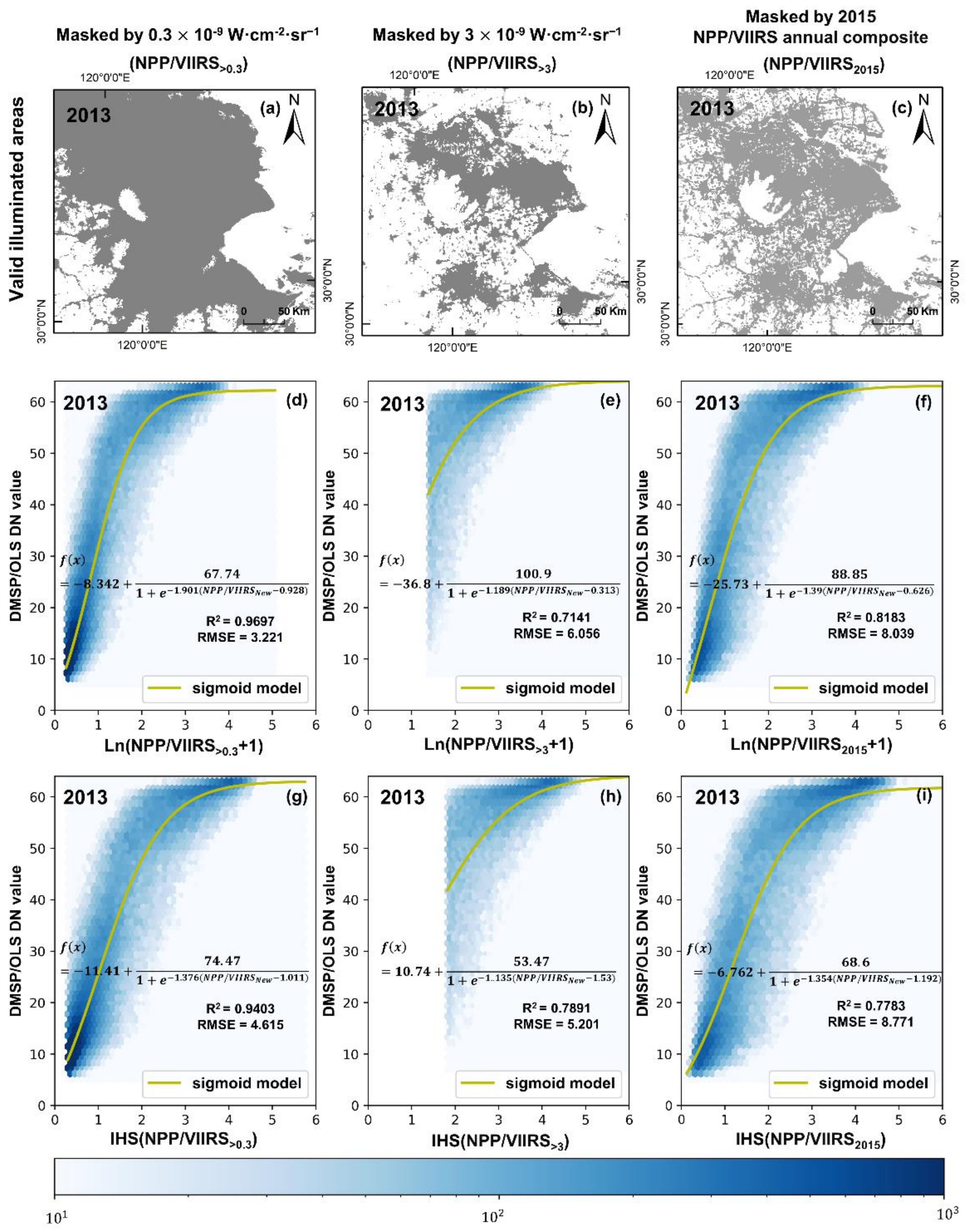
Three background noise mask methods were selected for defining the upper/lower limits to exclude background noise, gas, and fire cases (see Figure 2a–c): (a) an absolute lower limit (0.3 × 10⁻⁹ W·cm−2·sr−1) and a relative upper limit (the city core) (referred as T0.3 hereafter; see [24,30]; (b) an absolute lower limit (3 × 10⁻⁹ W·cm−2·sr−1) and a relative upper limit (the city core) (referred as T3 hereafter; see [40]); and (c) the limits from the NPP/VIIRS annual composite of 2015 (referred as T2015 hereafter; see [41,42]).

2.3. Data Assimilation

To obtain a consistent long nighttime light series, the approach developed by Zhao et al. [30] (or Gibson et al. [43]) is employed: first, a logarithmic (or inverse hyperbolic sine (IHS)) transformation is performed to adjust the range of the NPP/VIIRS data to be comparable with the DMSP/OLS data.
N P P / V I I R S N e w = l n N P P / V I I R S > T + 1   o r   N P P / V I I R S N e w = I H S N P P / V I I R S > T = l n N P P / V I I R S > T + N P P / V I I R S > T 2 + 1
Here NPP / VIIRS > T ( NPP / VIIRS New ) is the original (adjusted) NPP/VIIRS radiance value; the constant 1 ensure data consistency with transformed NPP/VIIRS nighttime light data greater than 0. T is the threshold for excluding background noise, gas, and fire cases. Then, the overlapping data (2013) from DMSP/OLS and NPP/VIIRS were selected to fit the coefficients a, b, c, and d for a sigmoid function comparison (see Figure 2).
f x = a + b 1 + e c log N P P / V I I R S N e w d

2.4. Threshold Setting for the Built-up Area

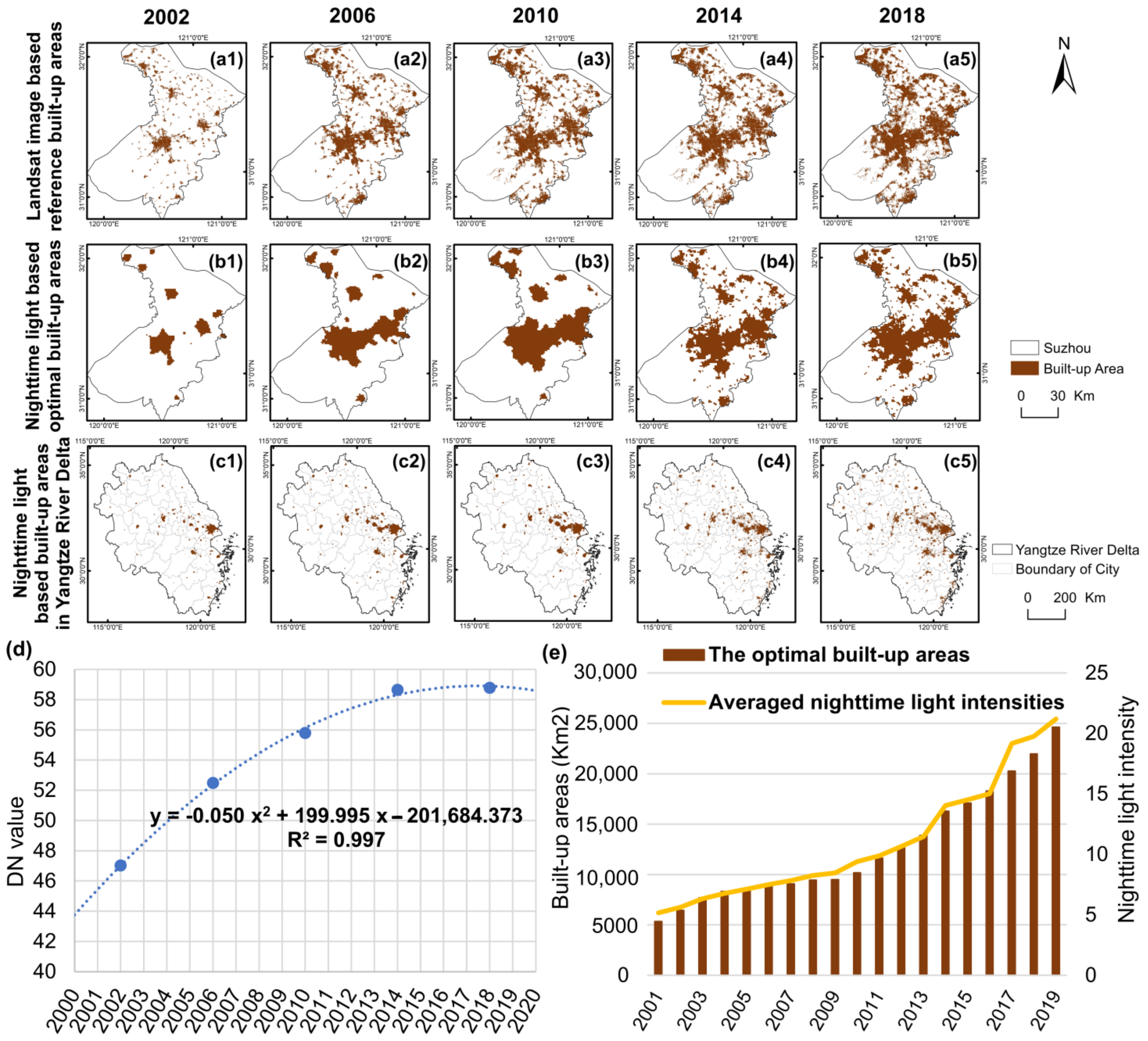
According to the method proposed by Small et al. [44] and Liu et al. [45], the optimal threshold is determined in 2002, 2006, 2010, 2014, and 2018 when area from DMSP/OLS and NPP/VIIRS nighttime light data closest to the area from the manual interpretation of the Landsat images (see Figure 3a,b). A quadratic regression with R2 = 0.997 was applied to set the threshold values for the remaining years (Figure 3d). The quadratic regression-based threshold values of 2013 and 2017 were selected and tested with built-up areas from the manual interpretation of the Landsat images (detailed accuracies see Section 3).

2.5. Area Tendency and Light Intensity Tendency

To estimate the long-term urban agglomeration development, a linear regression analysis (against year from yr = 1, 2, …n) was employed to determine x, the area tendency and light intensity tendency from the time development on city scale and pixel scale. The results are subjected to an F-test with all significance levels on the p-value < 0.05 level (unless noted otherwise).
  t e n d e n c y x = n y r = 1 n y r x y r y r = 1 n y r y r = 1 n x y r n y r = 1 n y r 2 y r = 1 n y r 2

2.6. Hot and Cold Spot Analysis

The Getis-Ord Gi* statistic has been widely adopted to analyze biological habitat [46], epidemic disease [47], and crime [48] to identify the significant spatial clusters of high values (hot spots) and low values (cold spots), which characterize the intensity of the geographic relation between observed data within a region. This functionality has been included in the automatic output of the hot spot analysis (Getis-Ord Gi*) tool in ArcGIS software [49], and is calculated as follows:
G i i * Z = j = 1 n w i , j x j X ¯ j = 1 n w i , j S n j = 1 n w i , j 2 j = 1 n w i , j 2 n 1
w i t h   w i , j = 1 ,   d i s t a n c e   t o   x j < 100   km   o r   3   km   0 ,   d i s t a n c e   t o   x j > 100   km   o r   3   km
and X ¯ = j = 1 n x j / n and S = j = 1 n x j 2 / n X ¯ 2 .
G i i *   Z is the Getis-Ord Gi* statistical z-score value for an administrative city or a pixel i, which describes the spatial dependency of i on all the surrounding administrative cities or pixels j. x j represents the magnitude of area tendency or light intensity tendency at location j, and X ¯ is the averaged magnitude over all the cities or pixels n. w i , j is the spatial weight value between the administrative city or pixel i and j, whose value equals either 1 or 0 defined by the distance between i and j. In this study, distances of 100 km and 3 km were selected for city scale and pixel scale, respectively. Clusters of high values (hot spots) and low values (cold spots) passing the 90% confidence level were categorized from the long-term tendencies of nighttime light intensity and area coverage. For a detailed method description see [50] and https://desktop.arcgis.com/en/arcmap/10.3/tools/spatial-statistics-toolbox/h-how-hot-spot-analysis-getis-ord-gi-spatial-stati.htm (accessed on 11 January 2021).

2.7. Tendency Shift

Pettitt’s test is a non-parametric test for detecting the tendency shift in a time series [51]. Here it was applied to the time series of the built-up areas and nighttime light intensities with the null hypothesis that there is no tendency shift or change-point in a time series. The test statistic K t , N and the associated probability P are given. Years in the time series with P t 0   0.05 were considered to be statistically significant change-points in a given time series.
K t , N = m a x i = 1 t j = t + 1 N s g n x i x j   ,   1 t < N
P t 0 = 2 e x p 6 K t , N 2 / ( N 3 + N 2 )
where s g n x i x j = 1 ,   x i x j > 0 0 ,   x i x j = 0 1 ,     x i x j < 0 .

3. Results

3.1. Background Noise Mask and Data Assimilation

Areas of three background noise masks indicate T0.3 > T2015 > T3 for the Yangtze River delta. Gibson [42] indicates that using the NPP/VIIRS annual composite for 2015 (T2015) as the background noise mask has the advantage of creating a like-with-like series to link to DMSP/OLS (because the NPP/VIIRS annual composite was processed to the same standard as the DMSP/OLS composite). However, when applying the sigmoid regression after the logarithmic and IHS transformation to the masked NPP/VIIRS data in 2013 (Figure 2), the results indicate that ln(NPP/VIIRS > 0.3 + 1) performs with a higher R2 value of 0.9697 (see Figure 2). Thus, the logarithmic transformation was used in the following analysis.

3.2. Threshold Setting for the Built-Up Areas

The nighttime light based built-up areas and their thresholds in Suzhou from 2001 to 2019 were extracted with the methods presented in Section 2 based on the manual interpretation of the Landsat images in 2002, 2006, 2010, 2014, and 2018 (see Figure 3). Accuracy test between nighttime light based built-up areas and Landsat images interpreted areas in the years 2013 and 2017 shows overall accuracies of 92.99% and 92.19% with Kappa coefficients of 0.67 and 0.66, respectively. That is, the selected thresholds for built-up regions extraction in the present study have credibility. Therefore, the spatiotemporal evolution of the built-up regions in Yangtze River Delta is extracted based on the threshold from Figure 3d. The following results are noticed (see also Figure 3e):
(1) Nighttime light intensity thresholds for DMSP/OLS indicate a systematic shift from 1 per year between 2000 and 2012 (thresholds change from 44 to 57), while NPP/VIIRS data are much more stable with the threshold value 58 after 2013. (2) Area expansion (averaged nighttime light intensity) increased by four to five times from 5000 km2 in 2001 to 24,000 km2 in 2019 (from 5.18 in 2001 to 21.2 in 2019). (3) Two stage transforms from moderate to fast developments of the built-up areas and the averaged nighttime light intensity were divided around 2010, and further detailed explanations about the most frequent shifted years with Pettitt’s test see Section 4.3.

3.3. Accuracy Test with MODIS Data

Shi et al. [20] reported that for 12 Chinese cities, thresholds vary from 2.9 to 23.7 × 10⁻⁹W·cm−2·sr−1 (or DN from 22 to 61). Thus, a further accuracy test comparing our threshold based built-up area with the urban built-up area from MODIS Land Cover products (MODIS 12Q1, 500 m spatial resolution) in 2005, 2010, and 2015 (see Table 1) was calculated, to test whether the threshold of Suzhou was representative for deriving urban extent for all the cities over the Yangtze River Delta. The results show overall accuracy reaching 97.56%, 97.29%, and 95.49% with Kappa coefficients of 0.66, 0.68, and 0.65, respectively.

4. Analyses and Discussion

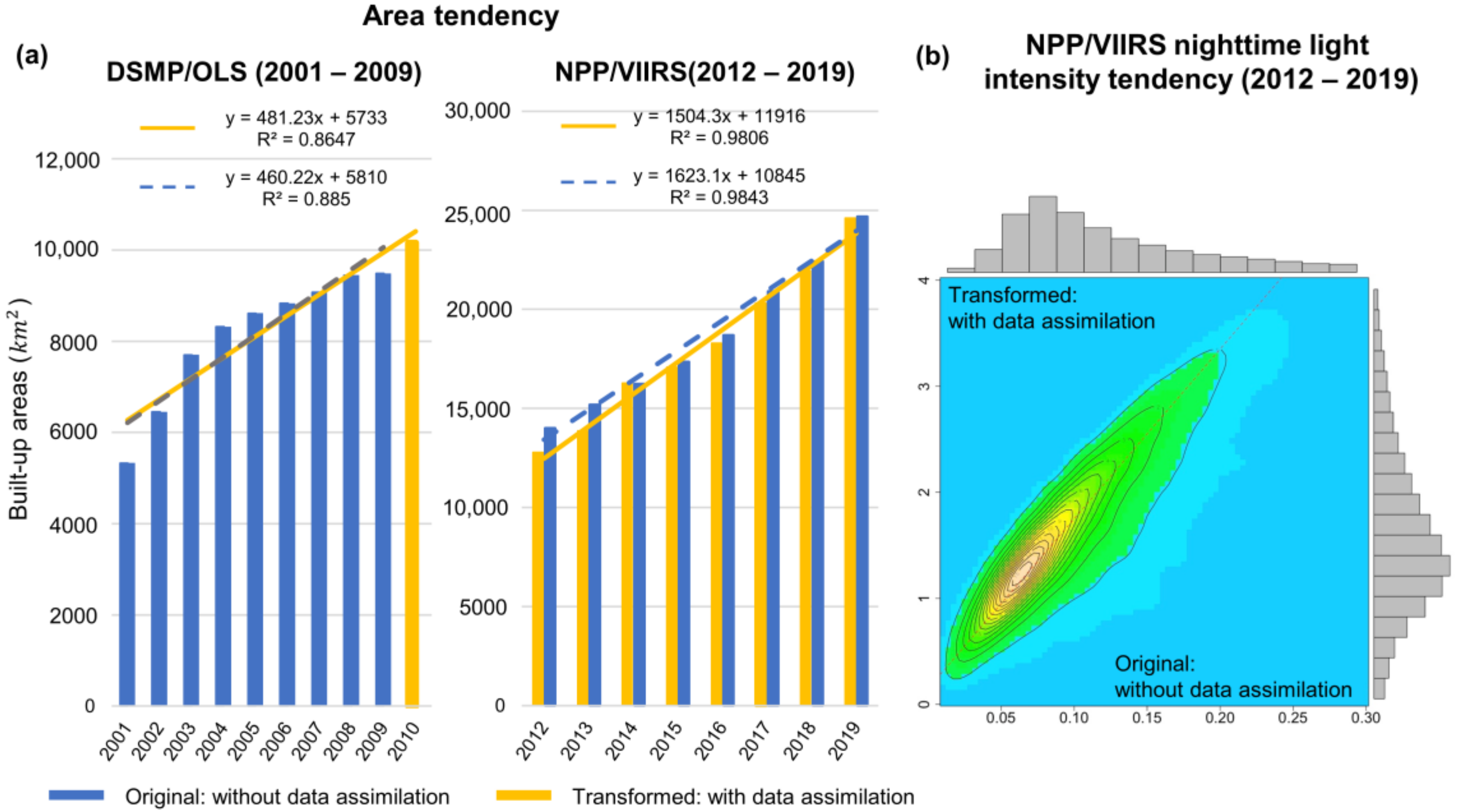
DMSP/OLS data F18 2010-2013 are considered problematic, because it records much higher DN values than earlier DMSP/OLS satellites [52]. Results from splitting the data into two decades (that is, 2001–2010 and 2011–2019) might be affected rather by different sources of nighttime light data than by inherent urban and nighttime light change tendencies. A sensitivity test, to exclude the possible lacking assurance from (1) satellite differences, (2) sensor drawbacks, and (3) data assimilation, is designed by calculating the original (excluding F18 and without data assimilation) area and/or nighttime light intensity tendencies of the DMSP/OLS data in 2001–2009 versus the NPP/VIIRS data in 2012–2019 (also without F18 and data assimilation; Figure 4).
In built-up area detection (Figure 4a), the possible drawbacks from satellite, sensor, and data assimilation are excluded because, instead of using a constant nighttime light threshold, the optimal thresholds are determined in 2002, 2006, 2010, 2014, and 2018 when area from DMSP/OLS and NPP/VIIRS nighttime light data were closest to the area from the manual interpretation of the Landsat images. Accuracy tests in 2013 and 2017 with built-up areas from the manual interpretation of the Landsat images show overall accuracies of 92.99% and 92.19% with Kappa coefficients of 0.67 and 0.66. In addition, the area tendency ratios of NPP/VIIRS to DMSP/OLS with versus without data assimilation were similar and about 3 (1504/481 km2/year = 3.12 versus 1623/460 km2/year = 3.52).
The NPP/VIIRS nighttime light intensity tendencies with/without data assimilation are compared (2012–2019) and presented as a frequency (number density) distribution in Figure 4b. Despite regional deviations, the NPP/VIIRS light intensity tendencies with/without data assimilation over the Yangtze river delta were almost linear. That is, the possible drawbacks from satellite, sensor, and data assimilation show less sensitivity in the following tendency analysis. Therefore, two periods (2001–2010 versus 2011–2019) were analyzed over the Yangtze River Delta, with built-up area tendency on administrative city scale (Section 4.1), nighttime light intensity tendency on pixel scale (Section 4.2), and in spatiotemporal joint analysis combining tendencies of built-up area and nighttime light intensity (Section 4.3).

4.1. Spatial Heterogeneity in the Administrative City Scale

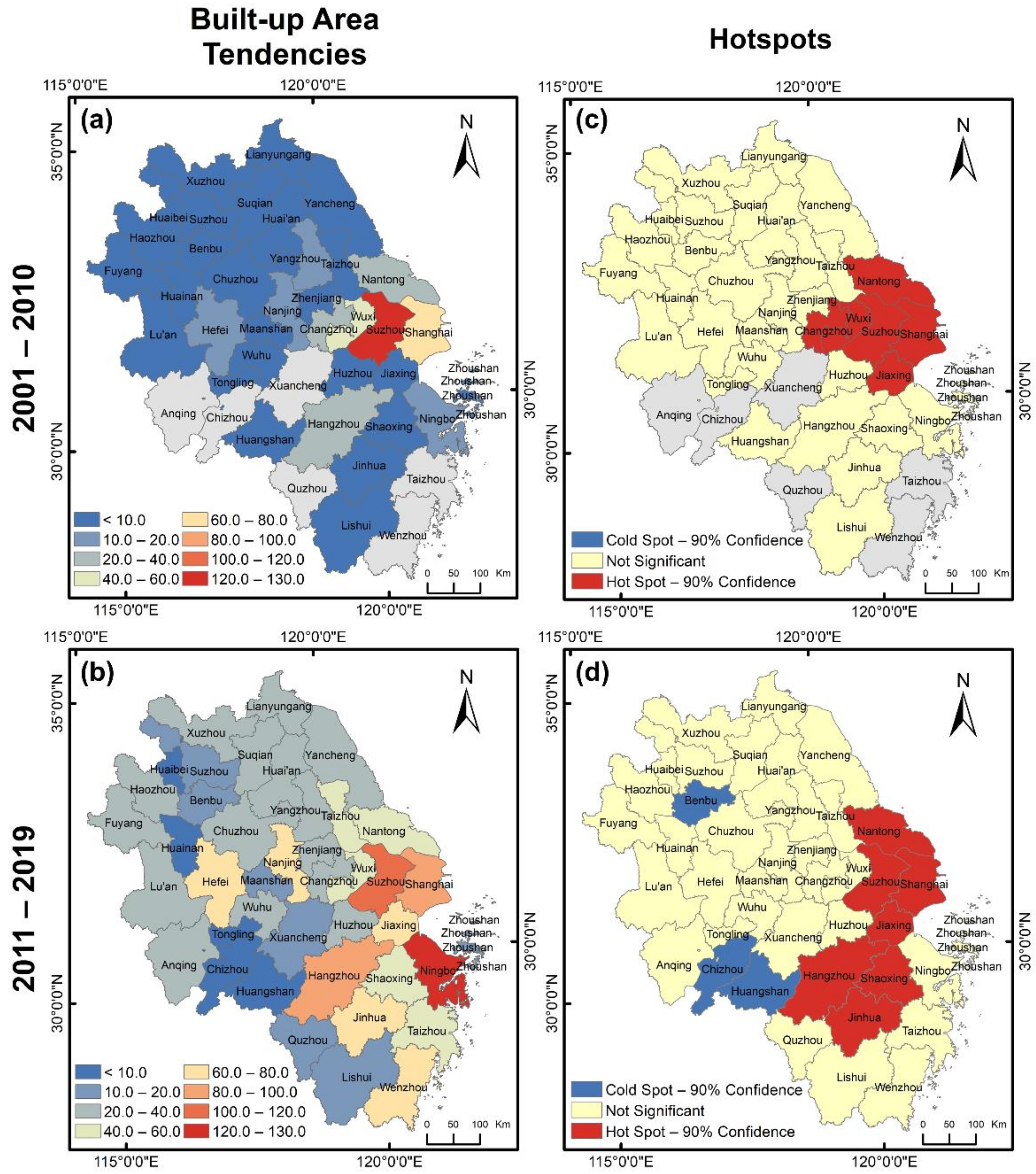
The built-up areas in each city of Yangtze River Delta from 2001 to 2019 are extracted with the threshold presented in Figure 3d. A linear regression is applied to the built-up area time series of each city and the tendencies with significance p-value < 0.05 are used for a further hot and cold spot analysis (Figure 5).
In the first period of 2001–2010 (Figure 5a), a rapidly increasing tendency of the built-up area could be diagnosed as a scattered distribution center around the core city of Shanghai, from a fast to a slow development Suzhou > Shanghai > Wuxi > Changzhou with the associated tendency values 126.94 > 66.84 > 42.53 > 32.29 km2/year, respectively. While cities far away from Shanghai like Anqing, Chizhou, and Xuanchen in the Southern Anhui province, and Quzhou, Wenzhou, and Taizhou in the Southern Zhejiang province show no significant increasing tendencies of built-up area. In the second period of 2011–2019 (Figure 5b), the rapidly increasing tendencies clustering the surrounding cities into one metropolitan domain, which means that cities close to Shanghai and along the costal line undergo a rapid built-up area expansion, with Ningbo > Suzhou > Hangzhou > Shanghai revealing tendency values 121.81 > 109.05 > 91.86 > 87.69 km2/year. Inner land cities with a relatively long distance to Shanghai show lower tendency values of urban spatial expansion, that is Huangshan < Chizhou < Tongling < Huainan < Huaibei with the tendency values 0.78 < 3.26 < 7.33 < 9.01 < 9.36 in Anhui Province. All the findings are in agreement with “the Riverside Development Belt”, “the Shanghai-Hangzhou-Jinhua development belt”, and “the coastal development belt” development plan (2015–2030) [53].
Hot spot and cold spot distributions for the two periods highlight the significant spatial clusters of high area tendency values (hot spots) and low area tendency values (cold spots). In the first period of 2001–2010 (Figure 5c), the hotspots of built-up area tendencies are clustered around the core city Shanghai (as a concentration distribution), surrounded by Suzhou, Wuxi, Changzhou, Nantong, and Jiaxing, which is consistent with a previous study [54]. By contrast, in the second period of 2011–2019 (Figure 5d), the hotspot areas were no longer clustered with the core city Shanghai but spreading to the southern regions of the Yangtze River Delta. Hangzhou, Shaoxing, and Jinhua from Zhejiang province replacing Wuxi and Changzhou bloom in terms of the built-up area. That is the spatial form of integrated cities from several provinces (or urban agglomeration) was noticed (see also Figure 5b and [55,56]). Cold spots locate on Bengbu, Chizhou, and Huangshan, Anhui province, which may be related to floods, population exodus, and low industrialization in Northern Anhui [57], and mountainous area limitation and natural landscape protection (Huangshan National Forest Park) in Southern Anhui [58].

4.2. Temporal Heterogeneity in the Pixel Scale

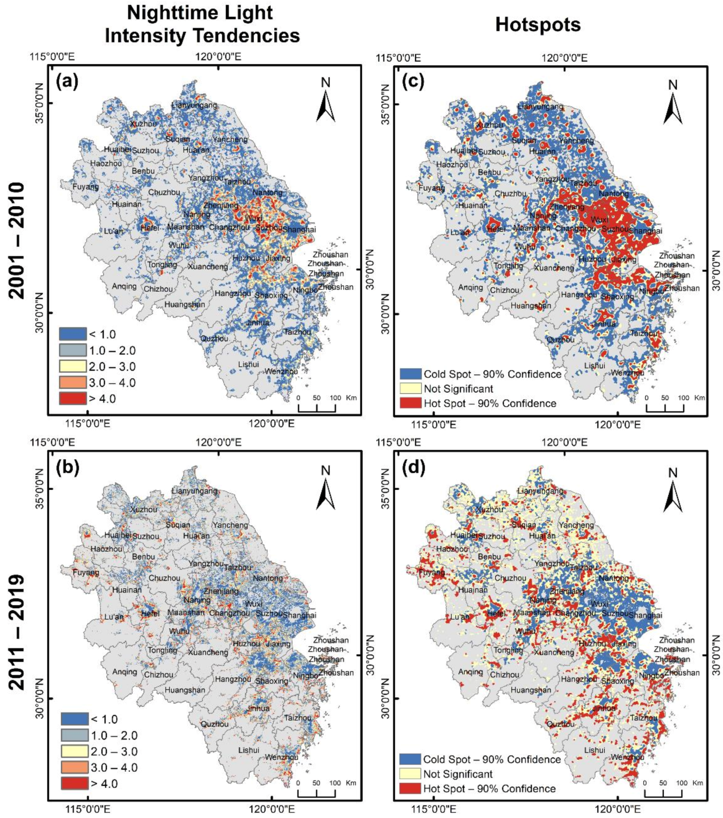
As nighttime light intensity is closely related to electricity consumption, it has been used as an indicator of the growth of built-up areas. The linear nighttime light intensity tendencies of significance (p-value < 0.05) over Yangtze River Delta were calculated for a further hot and cold spot analysis (Figure 6) and show the following results:
From the first to the second period, spatial heterogeneity of a “rapid to moderate” and a “moderate to rapid” increasing tendency could be diagnosed. In the period of 2001–2010 in Figure 6a (2011–2019 in Figure 6b), rapid (moderate) increasing tendencies of the nighttime light intensity are concentrated as a cluster around Suzhou surrounded by Wuxi, Jiaxing, Changzhou, and Shanghai, with averaged nighttime light intensity tendency values of 2.50 > 2.15 >1.87 > 1.84 > 1.61 (1.04, 1.06, 1.78, 1.48, 0.94) per year. In contrast, inner cities in Zhejiang province, Quzhou, Huzhou, Jinhua, and Zhoushan have been undergoing a “moderate to rapid” transition increasing from 0.58, 0.92, 0.93, 1.23–1.80, 1.85, 1.80, and 2.08 per year in terms of the averaged nighttime light intensity tendencies (2001–2010 versus 2011–2019). Similarly, inner cities in Anhui province, Chuzhou, Anqin, Lu’an, and Bengbu have increased from 0.60, 0.68, 0.68, 0.69–1.74, 1.64, 1.84, and 1.62 per year.
Hot spot and cold spot distributions for the two periods highlight the significant spatial clusters of high nighttime light intensity tendency values (hot spots) and low nighttime light intensity tendency values (cold spots). Heterogeneity of a “hot to cold” and a “cold to hot” spatial distribution could be diagnosed. In the first period of 2001–2010 (Figure 6c), the statistically significant hotspots of nighttime light intensity tendency are mainly concentrated around Suzhou with a “Z”-shape distribution as mentioned in previous studies [56,59], surrounded by cold spots in its suburbs and the countryside. In contrast, for the period of 2011–2019 (Figure 6d), the statistically significant cold spots of the nighttime light intensity tendency occupied the “Z”-shape, including Shanghai, Suzhou, Wuxi, Changzhou, Hangzhou, and Ningbo.

4.3. Spatial-Temporal Joint Analysis

Two periods’ hot spot and cold spot analyses (2001–2010 versus 2011–2019) over the Yangtze River Delta with built-up area tendency in administrative city scale (Section 4.1) and nighttime light intensity tendency in pixel scale (Section 4.2) list cities with high and low tendency values. To further diagnose (1) the tendency shift in the time series and (2) the total gross domestic product (GDP) associated spatiotemporal variability in the 41 administrative cities over Yangtze River Delta. Pettitt’s test [51] is applied to the time series of the built-up areas and nighttime light intensities, and then 41 administrative cities are categorized based on local total gross domestic product, into fast-developing cities, moderate-developing cities and slow-developing cities. Jenks Natural Breaks Classification Method [60] is applied to make sure within category are more similar than the between category.

4.3.1. Tendency Shift Detection

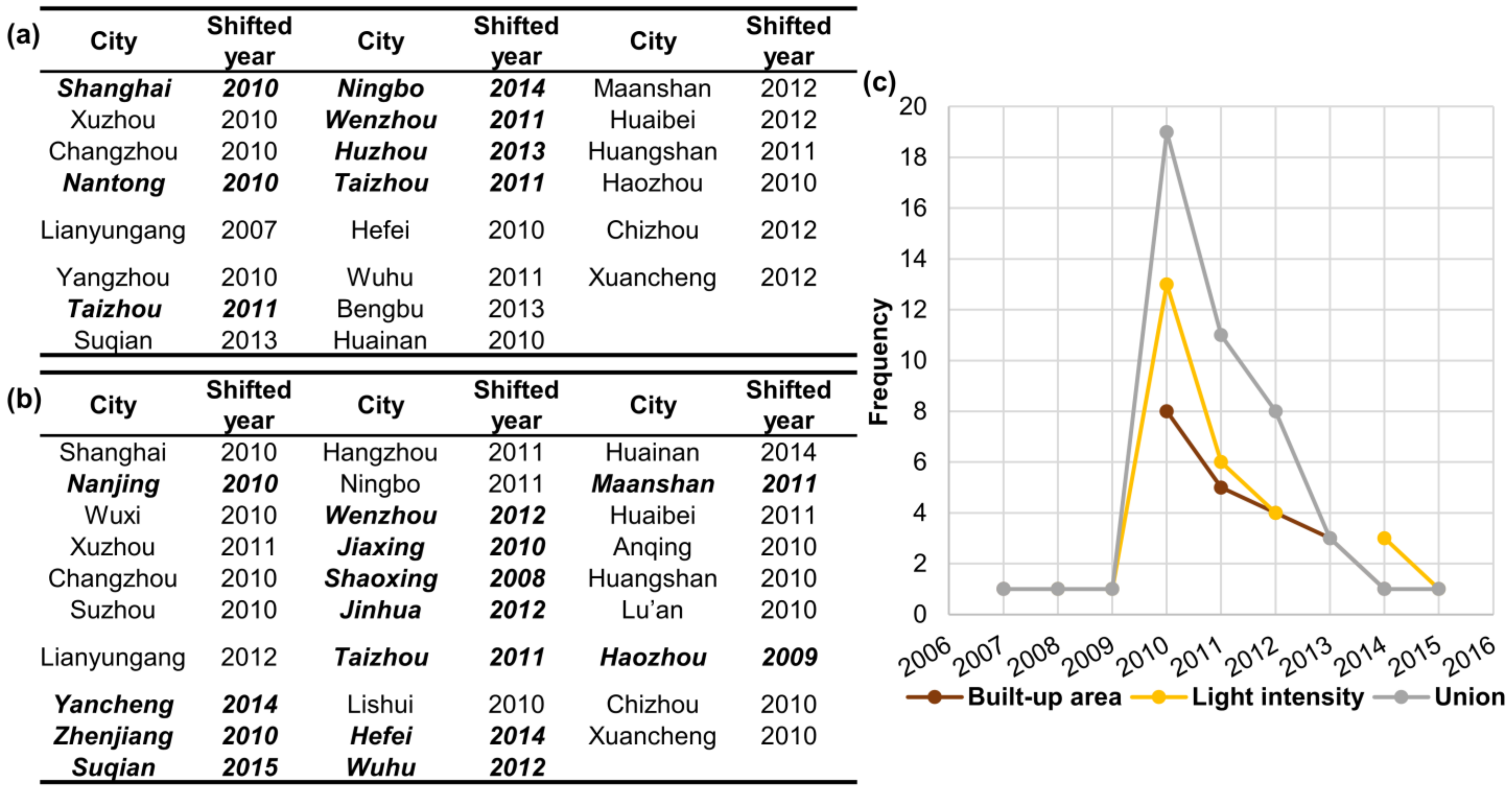
In the urbanization process of southward development and several inner cities’ booming, 22 (29) cities undergo statistically significant tendency shifts in terms of the annual built-up area (nighttime light intensity) (Figure 7). Years with statistically significant tendency shifts occur most frequently in 2010: in total, 19/41 cities show the tendency shift for built-up area (8/41 cities) or nighttime light intensity (13/41 cities). In the Yangtze River Delta, the cities with statistically significant tendency shift belong to the hot spot cities (see Figure 5d and Figure 6d) are highlighted in bold (Figure 7a,b) emphasizing both a southward and an inner cities’ development.

4.3.2. GDP Associated Spatiotemporal Variability

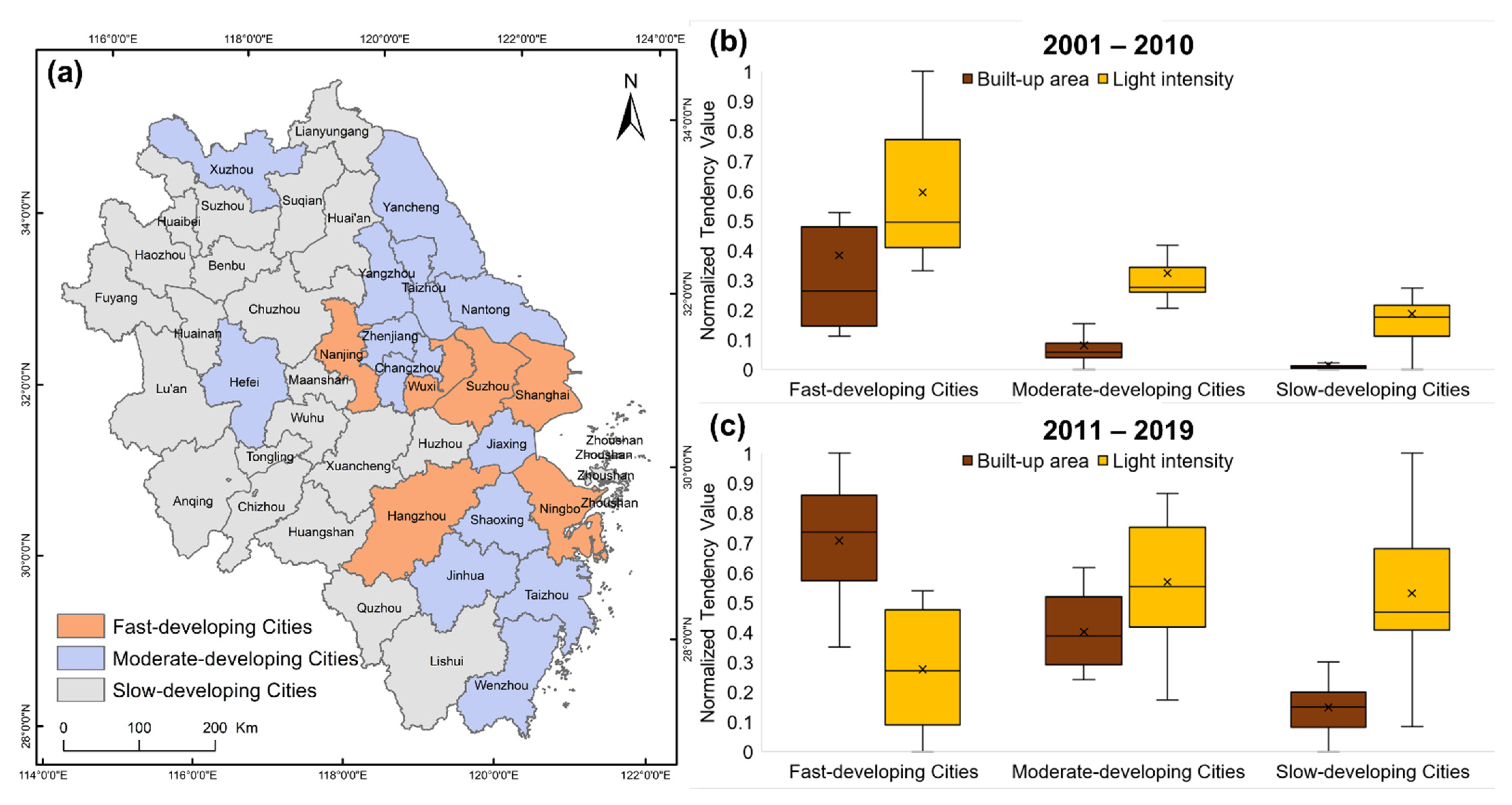
Gross domestic product (GDP) is an indicator of economic activity, which closely relates to the development level of a region and has a strong correlation with nighttime light intensity [61]. Thus, fast-, moderate-, and slow-developing cities were categorized according to the total GDP (2001–2018) of the 41 cities in Yangtze River Delta (Figure 8). The normalized statistics provide the following information:
(1) The fast-developing cities show an increase (decrease) of the built-up area (nighttime light intensity) tendency from the first to the second period, with 0.14–0.47 to 0.57–0.85 (0.40–0.77 to 0.08–0.47). (2) The moderate- and slow-developing cities increase both in the built-up area and the nighttime light intensity tendency, with 0.03–0.08 to 0.29–0.51 and 0–0.06 to 0.08–0.19 in terms of built-up area tendency, 0.25–0.34 to 0.41–0.75 and 0.11–0.21 to 0.40–0.67 in terms of nighttime time light intensity tendency. (3) Comparing fast-, moderate-, and slow-developing cities in the first period, the increases of nighttime light intensity tendency all exceed the increases of built-up area. In the second period, the increases of the built-up area tendency in moderate- and slow-developing cities are still less than the increases of the nighttime light intensity tendency. However, the increases of the built-up area tendency in fast-developing cities overwhelm the increases of the nighttime light intensity tendency due to the nighttime light saturation in the city cores and a fast expansion to suburbs and countryside.
In summary, in the first period of their evolution, fast-developing cities were dominated by increasing nighttime light intensity, while in their second period this increase was shifted to an increase of the built-up area. The increases of the built-up area tendencies were positively related to the GDP, showing fast > moderate > slow city development, and the growth of built-up areas lagged behind the growth of light intensity. The “fast to slow” transition of the nighttime light intensity tendency indicates whether the city core was fully developed. In this sense, moderate- and slow-developing cities show potential for a “fast to slow” conversion of the nighttime light intensity tendency in the future.

5. Conclusions

The global urbanization process, where human population, material demands of production, human consumption, and urban waste discharge expand and become more intense, has recently emerged as a sustainability challenge in an increasingly urbanized world, particularly for more rapidly changing developing countries [62]. Nighttime light signals derived from the Defense Meteorological Satellite Program’s Operational Line scan System (DMSP/OLS) first provide striking remotely sensed data to analyze spatiotemporal changes in global urbanization processes [63]. Then, the Suomi National Polar orbiting Partnership Visible Infrared Imaging Radiometer Suite (NPP/VIIRS) nighttime light data of much higher quality than the nighttime light data from the DMSP/OLS are used to quantify the relationship between night lighted areas and urbanization variables, including urban expansion [22], population growth [64], electric power consumption [24], gross domestic product [42], and socioeconomic parameters [23,25]. However, to our knowledge, few studies have been concerned with the data assimilation from DMSP/OLS (data before 2013) to NPP/VIIRS (data after 2012) associated with a time changing threshold to define the built-up areas, but which is necessary due to considerable inconsistencies, different spatiotemporal quality, drawbacks of blooming effects and radiometric heterogeneities.
Thus, research on long-term changes of urbanization over rapidly changing Yangtze River Delta may provide insights in diagnosing how long-time spatiotemporal heterogeneities of the urban evolution so as to provide insights in predicting a further urban agglomeration on a regional and global scale. This study compares dynamics of urbanization in 2001–2010 and 2011–2019 in the city unit scale and pixel unit scale, and the main conclusions are as follows.
(1) Comparing the two periods of area expansion indicates a general increase of the built-up areas in the second period of 2011–2019, and its geographical development gradually moves southward in the Yangtze River Delta. The hierarchy of the urbanization process of focusing on the core city is less obvious in the second period. Suzhou–Wuxi–Changzhou, Hangzhou, Ningbo, Nanjing, and Hefei contribute a fast development in the urban agglomeration, which is in agreement with the development plans for the Yangtze River Delta (2015–2030) to construct a networked of spatial pattern distribution characterized by “one mega, five circles and four belts” [53].
(2) The development transitions of a “rapid to moderate” and a “moderate to rapid” and the “hot to cold” and a “cold to hot” distribution indicate a continuous urban expansion. That is, regional development is first associated with a rapid increasing light intensity in the core cities, until the saturation of the light intensity. Then the rapidly increasing light intensity spills over, and thus accelerates the development of the surrounding suburbs and countryside in terms of both built-up area and light intensity. Likewise, the development of the surrounding suburbs and countryside appear to repeat this kind of development process “rapid to moderate” or “hot to cold”, which spills over (once more) when the nighttime light intensity saturated.
(3) The tendency shift of the built-up areas and nighttime light intensities for the 41 administrative cities over Yangtze River Delta occurs mainly in the year 2010, which indicates a decade as a characteristic time scale of urban evolution. Thereafter, the urban development characteristic has changed from a centralized pattern to a scattered distribution and undergoes an urban agglomeration process. In the process, the development time sequence is first the light intensity growth and then built-up area growth. In a developed (developing) city core, light intensity tendency is less (greater) than the built-up area tendency.
In general, urbanization is one of the extreme processes in land use and land cover change. Urbanization induced change of in surface parameters, including increased atmospheric greenhouse gas concentration, aerosol emissions, and land use and land cover change, is a major component for the formation and evolution of urban climates [65,66,67]. It accounts for effects like the urban heat island [68,69], affecting not only local and regional climates, but also water resources, air quality, human health, and biodiversity and ecosystem functioning [70]. Thus, research on the long-time evolution process of global/regional urbanization may provide insights in addressing the environmental problems arising from long-term and rapid urbanization and strengthening global or regional sustainable urban planning and management.

Author Contributions

M.Y., S.G., Y.G., and D.C. conceived and designed the experiments; M.Y., S.G., Y.G., and D.C. performed the experiments; M.Y., S.G., Y.G., and D.C. analyzed the data; M.Y., Y.G., and D.C. wrote the paper; X.Z. and Z.T. provided the data, and all authors contributed to the revising of the manuscript. All authors have read and agreed to the published version of the manuscript.

Funding

This research was funded by the Strategic Priority Research Program of Chinese Academy of Sciences: grant number XDA23100504.

Acknowledgments

Support by the Strategic Priority Research Program of Chinese Academy of Sciences (XDA23100504, as a participator) and the Max Planck Fellow Group (DC and KF), are acknowledged. The authors appreciate the valuable comments of the four reviewers.

Conflicts of Interest

The authors declare no conflict of interest.

References

  1. Gottmann, J. Megalopolis or the urbanization of the northeastern seaboard. Econ. Geogr. 1957, 33, 189–200. [Google Scholar] [CrossRef]
  2. Taubenböck, H.; Wiesner, M.; Felbier, A.; Marconcini, M.; Esch, T.; Dech, S. New dimensions of urban landscapes: The spatio-temporal evolution from a polynuclei area to a mega-region based on remote sensing data. Appl. Geogr. 2014, 47, 137–153. [Google Scholar] [CrossRef]
  3. Florida, R.; Gulden, T.; Mellander, C. The rise of the mega-region. Camb. J. Reg. Econ. Soc. 2008, 1, 459–476. [Google Scholar] [CrossRef]
  4. Friedmann, J. Four Theses in the Study of China’s Urbanization. Int. J. Urban Reg. Res. 2006, 30, 440–451. [Google Scholar] [CrossRef]
  5. UN. World Urbanization Prospects: The 2018 Revision; UN: New York, NY, USA, 2019. [Google Scholar]
  6. Tan, M.; Li, X.; Xie, H.; Lu, C. Urban land expansion and arable land loss in China—A case study of Beijing–Tianjin–Hebei region. Land Use Policy 2005, 22, 187–196. [Google Scholar] [CrossRef]
  7. Deng, X.; Huang, J.; Rozelle, S.; Zhang, J.; Li, Z. Impact of urbanization on cultivated land changes in China. Land Use Policy 2015, 45, 1–7. [Google Scholar] [CrossRef]
  8. Tu, J.; Xia, Z.-G.; Clarke, K.C.; Frei, A. Impact of Urban Sprawl on Water Quality in Eastern Massachusetts, USA. Environ. Manag. 2007, 40, 183–200. [Google Scholar] [CrossRef] [PubMed]
  9. Houghton, R.; Hackler, J. Sources and sinks of carbon from land-use change in China. Glob. Biogeochem. Cycles 2003, 17. [Google Scholar] [CrossRef]
  10. Cai, D.; Fraedrich, K.; Guan, Y.; Guo, S.; Zhang, C. Urbanization and the thermal environment of Chinese and US-American cities. Sci. Total Environ. 2017, 589, 200–211. [Google Scholar] [CrossRef] [Green Version]
  11. Li, W.; Zhou, W.; Han, L.; Qian, Y. Uneven urban-region sprawl of China’s megaregions and the spatial relevancy in a multi-scale approach. Ecol. Indic. 2019, 97, 194–203. [Google Scholar] [CrossRef]
  12. Bai, X.; Shi, P.; Liu, Y. Society: Realizing China’s urban dream. Nat. News 2014, 509, 158. [Google Scholar] [CrossRef] [PubMed] [Green Version]
  13. Martin, R. Rebalancing the Spatial Economy: The Challenge for Regional Theory. Territ. Politics Gov. 2015, 3, 235–272. [Google Scholar] [CrossRef] [Green Version]
  14. Tian, G.; Liu, J.; Xie, Y.; Yang, Z.; Zhuang, D.; Niu, Z. Analysis of spatio-temporal dynamic pattern and driving forces of urban land in China in 1990s using TM images and GIS. Cities 2005, 22, 400–410. [Google Scholar] [CrossRef]
  15. Tian, G.; Jiang, J.; Yang, Z.; Zhang, Y. The urban growth, size distribution and spatio-temporal dynamic pattern of the Yangtze River Delta megalopolitan region, China. Ecol. Model. 2011, 222, 865–878. [Google Scholar] [CrossRef]
  16. Hu, H.Y. The Distribution of Population in China, With Statistics and Maps. Acta Geogr. Sin. 1935, 2, 33–74. [Google Scholar] [CrossRef]
  17. Chen, M.; Gong, Y.; Li, Y.; Lu, D.; Zhang, H. Population distribution and urbanization on both sides of the Hu Huanyong Line: Answering the Premier’s question. J. Geogr. Sci. 2016, 26, 1593–1610. [Google Scholar] [CrossRef]
  18. Qi, W.; Liu, S.; Zhao, M.; Liu, Z. China’s different spatial patterns of population growth based on the “Hu Line”. J. Geogr. Sci. 2016, 26, 1611–1625. [Google Scholar] [CrossRef]
  19. Cai, D.; Fraedrich, K.; Guan, Y.; Guo, S.; Zhang, C.; Zhu, X. Urbanization and climate change: Insights from eco-hydrological diagnostics. Sci. Total Environ. 2019, 647, 29–36. [Google Scholar] [CrossRef]
  20. Shi, K.; Huang, C.; Yu, B.; Yin, B.; Huang, Y.; Wu, J. Evaluation of NPP-VIIRS night-time light composite data for extracting built-up urban areas. Remote Sens. Lett. 2014, 5, 358–366. [Google Scholar] [CrossRef]
  21. Guo, W.; Lu, D.; Wu, Y.; Zhang, J. Mapping impervious surface distribution with integration of SNNP VIIRS-DNB and MODIS NDVI data. Remote Sens. 2015, 7, 12459–12477. [Google Scholar] [CrossRef] [Green Version]
  22. Wu, W.; Zhao, H.; Jiang, S. A Zipf’s Law-Based Method for Mapping Urban Areas Using NPP-VIIRS Nighttime Light Data. Remote Sens. 2018, 10, 130. [Google Scholar] [CrossRef] [Green Version]
  23. Xie, Y.; Weng, Q.; Weng, A. A comparative study of NPP-VIIRS and DMSP-OLS nighttime light imagery for derivation of urban demographic metrics. In Proceedings of the 2014 Third International Workshop on Earth Observation and Remote Sensing Applications (EORSA), Changsha, China, 11–14 June 2014; pp. 335–339. [Google Scholar]
  24. Shi, K.; Yu, B.; Huang, Y.; Hu, Y.; Yin, B.; Chen, Z.; Chen, L.; Wu, J. Evaluating the Ability of NPP-VIIRS Nighttime Light Data to Estimate the Gross Domestic Product and the Electric Power Consumption of China at Multiple Scales: A Comparison with DMSP-OLS Data. Remote Sens. 2014, 6, 1705–1724. [Google Scholar] [CrossRef] [Green Version]
  25. Ma, T.; Zhou, C.; Pei, T.; Haynie, S.; Fan, J. Responses of Suomi-NPP VIIRS-derived nighttime lights to socioeconomic activity in China’s cities. Remote Sens. Lett. 2014, 5, 165–174. [Google Scholar] [CrossRef]
  26. Li, X.; Xu, H.; Chen, X.; Li, C. Potential of NPP-VIIRS Nighttime Light Imagery for Modeling the Regional Economy of China. Remote Sens. 2013, 5, 3057–3081. [Google Scholar] [CrossRef] [Green Version]
  27. Shi, K.; Yu, B.; Hu, Y.; Huang, C.; Chen, Y.; Huang, Y.; Chen, Z.; Wu, J. Modeling and mapping total freight traffic in China using NPP-VIIRS nighttime light composite data. GIScience Remote Sens. 2015, 52, 274–289. [Google Scholar] [CrossRef]
  28. Shao, X.; Cao, C.; Zhang, B.; Qiu, S.; Elvidge, C.; Von Hendy, M. Radiometric calibration of DMSP-OLS sensor using VIIRS day/night band. In Proceedings of the Earth Observing Missions and Sensors: Development, Implementation, and Characterization III, Beijing, China, 13–15 October 2014. [Google Scholar]
  29. Li, X.; Li, D.; Xu, H.; Wu, C. Intercalibration between DMSP/OLS and VIIRS night-time light images to evaluate city light dynamics of Syria’s major human settlement during Syrian Civil War. Int. J. Remote Sens. 2017, 38, 5934–5951. [Google Scholar] [CrossRef]
  30. Zhao, M.; Zhou, Y.; Li, X.; Zhou, C.; Cheng, W.; Li, M.; Huang, K. Building a Series of Consistent Night-Time Light Data (1992–2018) in Southeast Asia by Integrating DMSP-OLS and NPP-VIIRS. IEEE Trans. Geosci. Remote Sens. 2020, 58, 1843–1856. [Google Scholar] [CrossRef]
  31. Ma, J.; Guo, J.; Ahmad, S.; Li, Z.; Hong, J. Constructing a New Inter-Calibration Method for DMSP-OLS and NPP-VIIRS Nighttime Light. Remote Sens. 2020, 12, 937. [Google Scholar] [CrossRef] [Green Version]
  32. Zhang, X.; Guo, S.; Guan, Y.; Cai, D.; Zhang, C.; Fraedrich, K.; Xiao, H.; Tian, Z. Urbanization and Spillover Effect for Three Megaregions in China: Evidence from DMSP/OLS Nighttime Lights. Remote Sens. 2018, 10, 1888. [Google Scholar] [CrossRef] [Green Version]
  33. Liu, Z.; Liu, S.; Qi, W.; Jin, H. Urban sprawl among Chinese cities of different population sizes. Habitat Int. 2018, 79, 89–98. [Google Scholar] [CrossRef]
  34. Deng, Y.; Qi, W.; Fu, B.; Wang, K. Geographical transformations of urban sprawl: Exploring the spatial heterogeneity across cities in China 1992–2015. Cities 2020, 105. [Google Scholar] [CrossRef]
  35. Jiang, F.; Liu, S.; Yuan, H.; Zhang, Q. Measuring urban sprawl in Beijing with geo-spatial indices. J. Geogr. Sci. 2007, 17, 469–478. [Google Scholar] [CrossRef]
  36. Ou, J.; Liu, X.; Li, X.; Li, M.; Li, W. Evaluation of NPP-VIIRS Nighttime Light Data for Mapping Global Fossil Fuel Combustion CO2 Emissions: A Comparison with DMSP-OLS Nighttime Light Data. PLoS ONE 2015, 10, e0138310. [Google Scholar] [CrossRef] [PubMed] [Green Version]
  37. Jing, X.; Shao, X.; Cao, C.; Fu, X.; Yan, L. Comparison between the Suomi-NPP Day-Night Band and DMSP-OLS for Correlating Socio-Economic Variables at the Provincial Level in China. Remote Sens. 2015, 8, 17. [Google Scholar] [CrossRef] [Green Version]
  38. Gibson, J.; Olivia, S.; Boe-Gibson, G. Night Lights in Economics: Sources and USES1. J. Econ. Surv. 2020, 34, 955–980. [Google Scholar] [CrossRef]
  39. Elvidge, C.; Ziskin, D.; Baugh, K.; Tuttle, B.; Ghosh, T.; Pack, D.; Erwin, E.; Zhizhin, M. A Fifteen Year Record of Global Natural Gas Flaring Derived from Satellite Data. Energies 2009, 2, 595–622. [Google Scholar] [CrossRef]
  40. Liao, L.B.; Weiss, S.; Mills, S.; Hauss, B. Suomi NPP VIIRS day-night band on-orbit performance. J. Geophys. Res. Atmos. 2013, 118, 12705–12718. [Google Scholar] [CrossRef]
  41. Gibson, J. Better Night Lights Data, For Longer*. Oxf. Bull. Econ. Stat. 2020. [Google Scholar] [CrossRef]
  42. Gibson, J.; Olivia, S.; Boe-Gibson, G.; Li, C. Which night lights data should we use in economics, and where? J. Dev. Econ. 2021, 149. [Google Scholar] [CrossRef]
  43. Gibson, J.; Datt, G.; Murgai, R.; Ravallion, M. For India’s Rural Poor, Growing Towns Matter More Than Growing Cities. World Dev. 2017, 98, 413–429. [Google Scholar] [CrossRef] [Green Version]
  44. Small, C.; Pozzi, F.; Elvidge, C. Spatial analysis of global urban extent from DMSP-OLS night lights. Remote Sens. Environ. 2005, 96, 277–291. [Google Scholar] [CrossRef]
  45. Liu, Z.; He, C.; Zhang, Q.; Huang, Q.; Yang, Y. Extracting the dynamics of urban expansion in China using DMSP-OLS nighttime light data from 1992 to 2008. Landsc. Urban. Plan. 2012, 106, 62–72. [Google Scholar] [CrossRef]
  46. Cleasby, I.R.; Owen, E.; Wilson, L.; Wakefield, E.D.; O’Connell, P.; Bolton, M. Identifying important at-sea areas for seabirds using species distribution models and hotspot mapping. Biol. Conserv. 2020, 241. [Google Scholar] [CrossRef]
  47. Gwitira, I.; Murwira, A.; Zengeya, F.M.; Shekede, M.D. Application of GIS to predict malaria hotspots based on Anopheles arabiensis habitat suitability in Southern Africa. Int. J. Appl. Earth Obs. Geoinf. 2018, 64, 12–21. [Google Scholar] [CrossRef]
  48. Ratcliffe, J.H. Damned If You Don’t, Damned If You Do: Crime Mapping and its Implications in the Real World. Polic. Soc. 2002, 12, 211–225. [Google Scholar] [CrossRef]
  49. Environmental Systems Research Institute. ArcGIS Desktop: Release 10; Environmental Systems Research Institute: Redlands, CA, USA, 2011. [Google Scholar]
  50. Getis, A.; Ord, J.K. The analysis of spatial association by use of distance statistics. In Perspectives on Spatial Data Analysis; Springer: Berlin/Heidelberg, Germany, 2010; pp. 127–145. [Google Scholar]
  51. Pettitt, A.N. A Non-Parametric Approach to the Change-Point Problem. J. R. Stat. Soc. Ser. C (Appl. Stat.) 1979, 28, 126–135. [Google Scholar] [CrossRef]
  52. Tuttle, B.; Anderson, S.; Elvidge, C.; Ghosh, T.; Baugh, K.; Sutton, P. Aladdin’s Magic Lamp: Active Target Calibration of the DMSP OLS. Remote Sens. 2014, 6, 12708–12722. [Google Scholar] [CrossRef] [Green Version]
  53. National Development and Reform Commission; Ministry of Housing and Urban-Rural Development. The Development Plan for the Yangtze River Delta Megaregion (2015–2030). Available online: https://www.ndrc.gov.cn/xxgk/zcfb/tz/201606/W020190905517021091604.pdf (accessed on 11 January 2021).
  54. Wang, L.; Zhao, P. From dispersed to clustered: New trend of spatial restructuring in China’s metropolitan region of Yangtze River Delta. Habitat Int. 2018, 80, 70–80. [Google Scholar] [CrossRef]
  55. Luo, J.; Xing, X.; Wu, Y.; Zhang, W.; Chen, R.S. Spatio-temporal analysis on built-up land expansion and population growth in the Yangtze River Delta Region, China: From a coordination perspective. Appl. Geogr. 2018, 96, 98–108. [Google Scholar] [CrossRef]
  56. Xu, D.; Hou, G. The spatiotemporal coupling characteristics of regional urbanization and its influencing factors: Taking the Yangtze River Delta as an example. Sustainability 2019, 11, 822. [Google Scholar] [CrossRef] [Green Version]
  57. National Bureau of Statistics. Anhui: Analysis and Thoughts on Economic Operation in Northern Anhui. Available online: http://www.stats.gov.cn/ztjc/ztfx/fxbg/200407/t20040713_14765.html (accessed on 11 January 2021).
  58. Xu, S. On the Management of World Heritage in China—The Evaluation and Renewal of Huangshan Model. Tour. Trib. 2002, 6, 11–18. [Google Scholar]
  59. Che, Q. Urban Spatial Expansion Process, Pattern and Mechanism in Yangtze River Delta. Acta Geogr. Sin. 2011, 66, 446–456. [Google Scholar]
  60. Jenks, G.F. The data model concept in statistical mapping. Int. Yearb. Cartogr. 1967, 7, 186–190. [Google Scholar]
  61. Sutton, P.C.; Elvidge, C.; Ghosh, T. Estimation of Gross Domestic Product at Sub-National Scales using Nighttime Satellite Imagery. Int. J. Ecol. Econ. Stat. 2007, 8, 5–21. [Google Scholar]
  62. Angel, S.; Parent, J.; Civco, D.L.; Blei, A.; Potere, D. The dimensions of global urban expansion: Estimates and projections for all countries, 2000–2050. Prog. Plan. 2011, 75, 53–107. [Google Scholar] [CrossRef]
  63. Elvidge, C.D.; Baugh, K.; Kihn, E.; Kroehl, H.W.; Davis, E. Mapping City Lights With Nighttime Data from the DMSP Operational Linescan System. Photogramm. Eng. Remote Sens. 1997, 63, 727–734. [Google Scholar]
  64. Chen, X.; Nordhaus, W. A Test of the New VIIRS Lights Data Set: Population and Economic Output in Africa. Remote Sens. 2015, 7, 4937–4947. [Google Scholar] [CrossRef] [Green Version]
  65. Grimm, N.B.; Faeth, S.H.; Golubiewski, N.E.; Redman, C.L.; Wu, J.; Bai, X.; Briggs, J.M. Global change and the ecology of cities. Science 2008, 319, 756–760. [Google Scholar] [CrossRef] [PubMed] [Green Version]
  66. Ren, G. Urbanization as a major driver of urban climate change. Adv. Clim. Chang. Res. 2015, 6, 1–6. [Google Scholar] [CrossRef]
  67. Wu, K.; Yang, X. Urbanization and heterogeneous surface warming in eastern China. Chin. Sci. Bull. 2013, 58, 1363–1373. [Google Scholar] [CrossRef] [Green Version]
  68. Landsberg, H.E. The Urban Climate; Academic Press: Cambridge, MA, USA, 1981. [Google Scholar]
  69. Oke, T.R. Boundary Layer Climates; Routledge: London, UK, 2002. [Google Scholar]
  70. Platt, R.H.; Rowntree, R.A.; Muick, P.C. The Ecological City: Preserving and Restoring Urban Biodiversity; University of Massachusetts Press: Amherst, MA, USA, 1994. [Google Scholar]
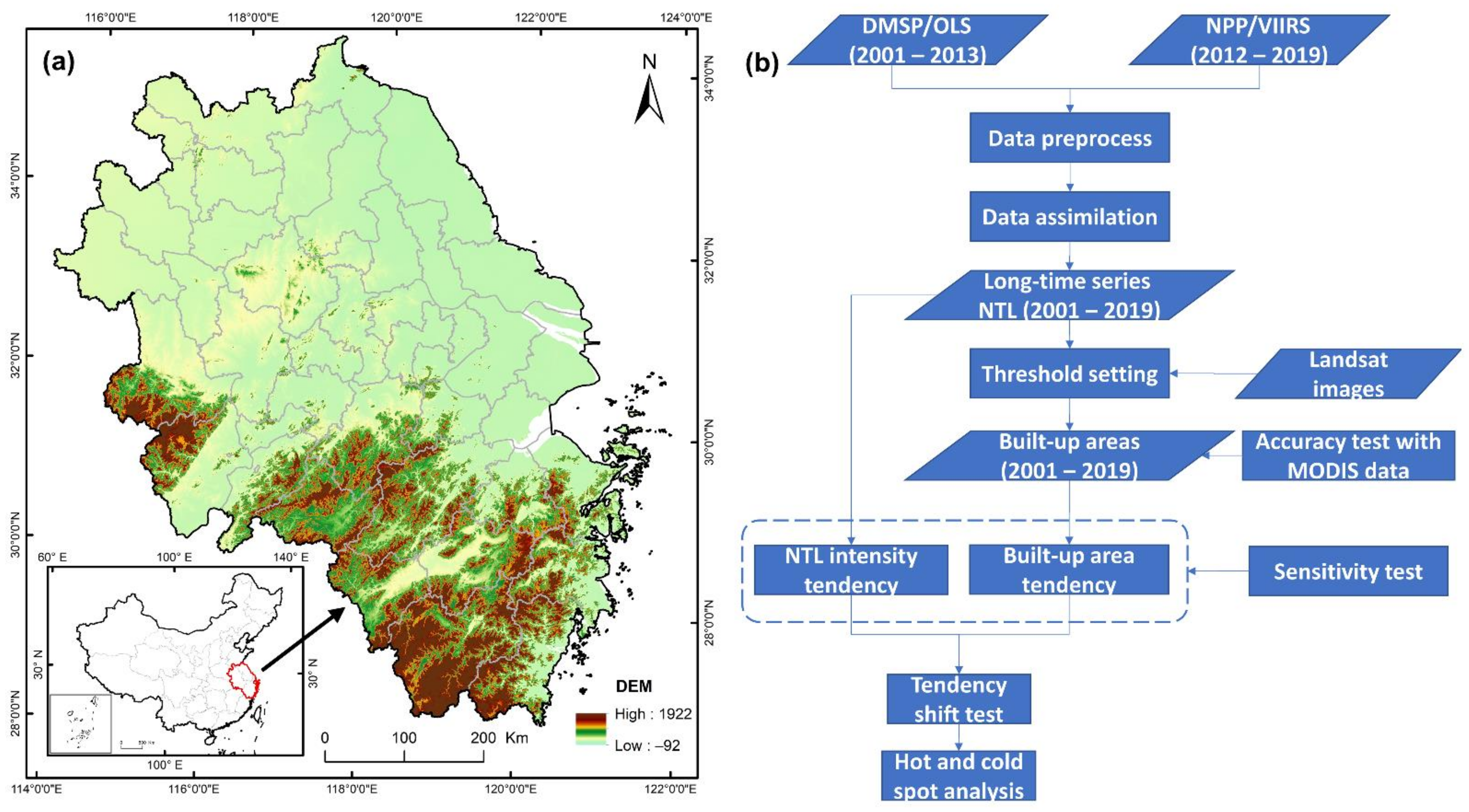
Figure 1. Geographical setting of the Yangtze River Delta (a) and application flowchart (b).
Remotesensing 13 01235 g001
Figure 2. Results from three background noise mask methods for defining the upper/lower limits: (a) an absolute lower limit (0.3 × 10⁻⁹ W·cm−2·sr−1) and a relative upper limit (the city core); (b) an absolute lower limit (3 × 10⁻⁹ W·cm−2·sr−1) and a relative upper limit (the city core); and (c) the limits from the NPP/VIIRS annual composite of 2015. Additionally, the corresponding sigmoid regression performance after applying the logarithmic (the middle row, df) and IHS transformation (the bottom row, gi) to the masked NPP/VIIRS data in 2013.
Remotesensing 13 01235 g002
Figure 3. Geographical settings of (a1a5) reference built-up areas from Landsat images, (b1b5) corresponding nighttime light based optimal built-up areas, and (c1c5) built-up areas extracted by the same nighttime light threshold over Yangtze River Delta. The optimum nighttime light threshold was determined according to (d) the non-linear fit of the threshold values (DN) in 2002, 2006, 2010, 2014, and 2018, within which built-up areas from the nighttime light data were most similar to the reference data in terms of the spatial area. Finally, (e) annual statistics of the built-up areas and averaged nighttime light intensities over the Yangtze River Delta (calculated for 2001–2019).
Remotesensing 13 01235 g003
Figure 4. The original (excluding F18 and without data assimilation, in blue) versus employing data assimilation (see Section 2, in yellow): (a) area and (b) nighttime light intensity tendencies of the DMSP/OLS data in 2001–2009 versus the NPP/VIIRS data in 2012–2019.
Remotesensing 13 01235 g004
Figure 5. Tendencies and hotspot detection in 2001–2010 and in 2011–2019 over the Yangtze River Delta: (a,b) linear regression tendencies of the built-up area and (c,d) hotspot analyses from the linear regression tendency.
Remotesensing 13 01235 g005
Figure 6. Tendencies and hotspot detection in 2001–2010 and in 2011–2019 over the Yangtze River Delta: (a,b) linear regression tendencies of the nighttime light intensity and (c,d) hotspot analyses from the linear regression tendency.
Remotesensing 13 01235 g006
Figure 7. Cities in the Yangtze River Delta: Statistics of tendency shift of the years with significant (95%) confidence: (a) built-up area change and (b) averaged nighttime light intensity change calculated by the Pettitt’s method; (c) related histogram of the tendency shifted years and hotspot cities in 2011–2019 are highlighted in bold (see also Figure 5d and Figure 6d).
Remotesensing 13 01235 g007
Figure 8. Based on the total gross domestic product, cities in Yangtze River Delta are divided into three regions: (a) the fast-, moderate-, and slow-developing cities. Statistics comparison over the three regions is calculated in terms of the tendencies of the normalized area and the nighttime light intensity between (b) 2001–2010 and (c) 2011–2019.
Remotesensing 13 01235 g008
Table 1. Accuracy test comparing nighttime light based built-up area with the urban built-up area from MODIS Land Cover products (MODIS 12Q1, 500 m spatial resolution) in 2005, 2010, and 2015.
200520102015
Overall accuracy (%)97.5697.2995.49
Kappa coefficient0.660.680.65
Publisher’s Note: MDPI stays neutral with regard to jurisdictional claims in published maps and institutional affiliations.