Abstract
Synthetic aperture radar (SAR) systems are susceptible to radio frequency interference (RFI). The existence of RFI will cause serious degradation of SAR image quality and a huge risk of target misjudgment, which makes the research on RFI suppression methods receive widespread attention. Since the location of the RFI source is one of the most vital information for achieving RFI spatial filtering, this paper presents a novel location method of multiple independent RFI sources based on direction-of-arrival (DOA) estimation and the non-convex optimization algorithm. It deploys an L-shaped multi-channel array on the SAR system to receive echo signals, and utilizes the two-dimensional estimating signal parameter via rotational invariance techniques (2D-ESPRIT) algorithm to estimate the positional relationship between the RFI source and the SAR system, ultimately combines the DOA estimation results of multiple azimuth time to calculate the geographic location of RFI sources through the particle swarm optimization (PSO) algorithm. Results on simulation experiments prove the effectiveness of the proposed method.
1. Introduction
As an active microwave remote sensing device, synthetic aperture radar (SAR) has achieved excellent performance in resource exploration, military reconnaissance, and other earth observation missions. However, the electromagnetic environment in which SAR works is becoming more complex, its working frequency bands are occupied by radio devices such as broadcasting and ground radar. For the SAR system, the signals emitted by these devices are generally called radio frequency interference (RFI) [1,2]. RFI usually causes bright lines and spots in SAR images, which dramatically degrades SAR image quality and masks targets of interest, severely weakens the performance of SAR [1,2,3,4,5]. Moreover, since strong RFI will cause a significant reduction in the signal-to-interference power ratio of the echo, we cannot accurately estimate the required radar parameters from it [2]. It is generally considered that RFI is a major challenge for SAR systems and RFI suppression becomes a necessary research topic [1,2,3,4,5,6,7].
In order to solve the RFI contamination problem, there are two main solutions to suppress RFI signals [3,4,5,6,7,8,9,10,11,12,13]. The first method is to use signal processing technology to find out the difference between RFI signal and the echo signal in the time or frequency domain, and design a filter to mitigate RFI [3,4,5,6,7]. In general, signal processing methods only utilize the signal characteristics of RFI to estimate and suppress interference. However, it is worth noting that this method can only achieve a good suppression effect in the case of accurately estimating some signal characteristics of RFI. Another method is to locate the RFI source based on the contaminated echo signal, and turn off the interference emitters or take advantage of beamforming technology to achieve spatial filtering [9,10,11,12,13]. This method mainly achieves the purpose of interference suppression by reducing the RFI signal entering the receiver. For the SAR system, taking into account the spatial characteristics of the interference signal, advanced SAR systems have the ability to adaptively adjust the antenna pattern for RFI mitigation, relying on the direction-of-arrival (DOA) of the interference signal, whose feasibility has been studied in some research [9,10]. Thus, it is greatly essential to get an accurate location of the RFI source for implementing this approach.
In the research on RFI location, the works focusing on DOA estimation were studied [7,11,12,13]. Among these research studies, References [7,11] studied the effective RFI source location methods for SAR systems. In [7], SAR images were used to record the azimuth time when the interference occurs, and on this basis, the location of RFI sources was estimated based on the scene location and the signal acquisition time. However, this method does not use the characteristics of the RFI signal and can only roughly locate the RFI. In Reference [11], a uniform linear array was designed to receive the signal, and then the multiple signal classification (MUSIC) algorithm was used for the array signal to realize a one-dimensional estimation of the direction of the RFI signal. Nevertheless, this method cannot obtain the two-dimensional angle of the RFI signal direction in the azimuth and elevation, so the two-dimensional pattern of the antenna cannot be designed based on the result to achieve RFI suppression, and the precise geographic location of the RFI source cannot be calculated. Besides, References [12,13] researched the RFI location for synthetic aperture interferometric radiometry (SAIR). Reference [12] used the MUSIC algorithm to achieve high-precision two-dimensional RFI DOA estimation. However, first of all, this work was proposed for SAIR, and the structure of the Y-shaped array designed in [12] is quite complicated for the SAR system. It is the virtual hexagonal array composed of 931 array elements, which is not suitable for SAR systems. Secondly, the two-dimensional MUSIC algorithm needs to use spatial spectrum search to complete DOA estimation, the computational complexity of this process is very high, which will greatly increase the computational burden of the system in practical applications [14,15]. Finally, this method only estimates the DOA of the RFI signal and does not calculate the geographic location of the RFI source, but the location information is important for detecting ground interference sources. The literature [13] is also a study on SAIR, the same as [12]. In addition, it introduces the spatial sparsity of RFI and considers that the spatial distribution of RFI sources obeys a prior Laplace probability function. This assumption is reasonable for the RFI source in SAIR, but there is no research showing that the RFI source in SAR also obeys similar distribution characteristics.
In order to calculate the exact geographic location of multiple RFI sources of SAR with taking into account the two-dimensional DOA estimation requirements and the complexity of the system calculation, this paper presents a new method for the location of multiple independent RFI sources combining two-dimensional estimating signal parameter via rotational invariance techniques (2D-ESPRIT) and the particle swarm optimization (PSO) algorithm. The main idea of this method is to employ array signal processing technology to estimate the spatial geometric relationship between the SAR system and the RFI sources at each azimuth time, and then use the particle swarm optimization method to solve the optimization problem in the geographic location estimation of multiple independent interference sources. This method is different from other methods in three main aspects. First of all, the proposed method makes use of an L-shaped channel array to realize the two-dimensional estimation of RFI DOA, its structure is simple and effective. The reason for choosing an L-shaped array is given in Section 2.1. Moreover, compared with the MUSIC algorithms, the two-dimensional ESPRIT used in this method does not need to construct and search the spatial spectrum of the signal, thereby reducing the computational burden and improving the computational efficiency of the DOA estimation method, which is very essential when processing large-scale SAR data. Last but not the least, the method of estimating the geographic location of RFI sources proposed in this paper can accurately indicate the specific geographic coordinates of RFI sources, instead of just getting the direction of RFI sources, which can provide location information for shutting down illegal RFI sources and help the SAR system avoid interference areas.
The rest of this paper is organized as follows. Section 2 describes the geometry model of the SAR system and RFI sources, the multi-channel array model, and the signal model. In Section 3, we present the multiple RFI sources geolocation method based on the 2D-ESPRIT and PSO algorithm under the condition of an L-shaped channel array. The simulation experiment given in Section 4 proves the feasibility of the proposed method, followed by the discussion and conclusion in Section 5 and Section 6.
2. Geometry and Signal Model
2.1. Geometry Model
For the SAR system, most RFI sources are related to electronic equipment on the surface of the earth [16]. Therefore, this paper establishes a simulation model of the normal working spaceborne SAR being simultaneously interfered with by multiple RFI sources on the ground. In the process of data acquisition, the SAR satellite moves in an elliptical orbit around the earth, and the antenna points to the imaging area on the side of the flight direction. Multiple RFI sources on the ground may exist in or outside the imaging area, which may make RFI signals enter the receiver from the main lobe of the antenna, or from the side lobes. Figure 1a shows the geometric model between the SAR system and multiple RFI sources when acquiring real echo signals and being interfered with by RFI signals in the east-north-up (ENU) coordinate system. It should be noted that, unless indicated, all geographic coordinates in this article are in the ENU coordinate system. The light yellow area on the ground shows the main beam coverage area of the SAR system antenna at the azimuth time of . As shown in this figure, there are some RFI sources on the ground that continuously transmit interference signals to the SAR system, and when the azimuth time is , the distance between the k-th interference source and the SAR system can be expressed as . During the data acquisition process, with the relative movement between the SAR system and RFI sources, the distance between them changes with the azimuth time. Figure 1b shows that the arrangement of the multi-channel array of the SAR system in Figure 1a.
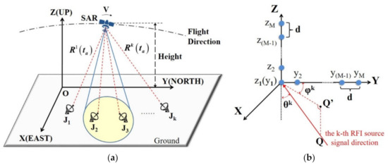
Figure 1.
The geometry model of signal acquisition of synthetic aperture radar (SAR) and the channel array arrangement: (a) The geometric relationship between the SAR system and multiple radio frequency interference (RFI)sources when the azimuth time is ; (b) The arrangement of the multi-channel array used by the SAR system in (a) and the definition of the elevation angle and the azimuth angle .
As can be seen from Figure 1b, (2M-1) channels are arranged at equal distance on the Y-axis and the Z-axis of the antenna coordinate system, and there are M channels on each axis and the distance between adjacent channels is d. Among them, the channel located at the origin of the coordinate belongs to the Y-axis and Z-axis arrays at the same time, and it is used to transmit and receive signals, while other channels only receive signals. Thus, at each azimuth time, the SAR system transmits signals through channel 1, and all channels receive echo signals. Moreover, we define the elevation angle and the azimuth angle of the k-th RFI signal as shown in Figure 1b. The purpose of DOA estimation is to estimate the value of these two angles.
The reason for choosing the L-shaped multi-channel array is as follows. First of all, different from the study of single interference source localization [17], in order to estimate the two-dimensional DOA of the interference signal at each azimuth time and apply it to multiple RFI sources geolocation, deploying multiple receiving channels as a non-linear array on the SAR system is necessary. Furthermore, for the SAR system, the accurate estimation of the geographic coordinates of the RFI source must be achieved based on multiple azimuth time DOA estimation results. Therefore, this method requires the system to have a good estimation accuracy of the direction of the RFI signal at each azimuth time. In addition, if the calculation complexity required for DOA estimation at each azimuth time is too high, the calculation burden of the system will be very heavy. Among various array models, the L-shaped array not only has the advantages of simple structure and low system design difficulty, but also it can offer a larger array aperture when the number of channels and the distance between channels is constant, which makes it have a higher DOA estimation accuracy [14,18]. Moreover, when processing the signal of the L-shaped array, we can simplify the two-dimensional DOA estimation problem into two independent one-dimensional DOA problems to solve [14,15], which will reduce the computational burden. Hence, considering the requirement of DOA estimation and the advantages of the L-shaped array, this paper proposes to arrange the multiple channels of the SAR system into an L-shaped to receive signals.
Besides, in order to achieve DOA estimation, the channels in the array should meet:
- All the channels are independent and isotropic.
- The distance between adjacent channels is not more than half the wavelength of the RFI signal.
2.2. Signal Model
According to the geometric model in Figure 1a, a SAR platform travels at a speed of , and continuously transmits a chirp signal and receives echo signals within the azimuth time. When the SAR system is interfered with, its echo signal is composed of the real target echo signal, RFI signal, and noise signal [1,2,3,4,5,6,7,8,9]. Thus, as the range time is and the azimuth time is , and RFI sources exist in the scene, the interfered echo signal received by each channel can be written as:
where denotes the interference signal from the k-th RFI source, and denote the real target echo signal and noise signal, respectively.
Due to the complex source of RFI, it is difficult to model it with a single signal form [2,3,4]. In terms of signal model, the form of sinusoidal modulation signal and linear modulation signal is simple and often used as the basic form of microwave radiation, which can be used to model RFI [2,3,4,5,6,7,8]. For the type of RFI, researchers usually classify RFI into narrowband interference (NBI) and wideband interference (WBI) according to the ratio of the RFI bandwidth to the echo signal bandwidth [2,3,4,5,6,7,8]. Furthermore, since the source of WBI is generally other radar systems, it can be modeled by the linear modulation signal whose parameters change over time [8], which is called wideband linear frequency modulated interference (WBLFMI) in this article. Meanwhile, NBI usually comes from communication equipment or television facilities with narrow bandwidth [4,5,6]. Compared with the bandwidth of SAR, this type of RFI signal may occupy a very narrow bandwidth in the frequency domain [8], or even occupy only one frequency bin like a sinusoidal signal [2]. Therefore, this article further divides NBI into narrowband linear frequency modulated interference (NBLFMI) and radio frequency noise interference (RFNI). This modeling method conforms to the signal characteristics of RFI in actual situations [2,3,4,5,6,7,8] and has achieved good results in the research on interference detection and suppression [19,20]. In addition, the pulse width of most RFI signals is shorter than the echo window time of SAR, which results in the RFI observed in actual data being pulsed [7,21]. Taking these factors into consideration, this article models the RFI signal as the pulsed signal, and these three types of interference are written as:
where , , and denote the amplitude of these three types of RFI signals, , , and are their pulse width, is the carrier frequency, is the frequency of RFNI, and are the chirp-rate of NBLFMI and WBLFMI, , , and denote the signal phase, is the distance between the k-th RFI source and the SAR system at the azimuth time of . In addition, it needs to be pointed out that the bandwidth of these three types of interference is relatively narrow compared to the bandwidth of the SAR signal [2,3,4,5].
Besides, in related research on RFI, the following assumptions are often mentioned generally:
- The real target echo signal, the RFI signal, and the noise signal are statistically independent [4,5].
- The RFI signal possesses dominant energy in the interfered echo signal, and the real target echo signal has a noise-like spectrum compared with the RFI signal, which means we can define the sum of the real target echo signal and noise signal as the equivalent additive noise [4,5,6]:
- RFI signals from different interference sources are uncorrelated [9,10,11,12,13].
- The antennas of each channel of the SAR system are isotropic and not coupled to each other [9,10,11,12,13].
- The distance between RFI source and the spaceborne SAR system usually meets the far field condition [9,10,11].
According to Equations (1) and (3), the contaminated echo signal received by the m-th channel on the Z-axis of the channel array of the SAR system can be expressed as:
where denotes the signal from the k-th RFI source received by this channel, denotes the equivalent additive noise composed of the sum of the real target echo signal and the noise signal.
At the same azimuth time, the interference signal from the k-th RFI source is received by channel , and its received signal can be expressed as . The relationship between and can be written as:
where denotes the time difference between the interference signal of the k-th RFI source reaching channel and channel . Since the RFI signal can be regarded as a narrowband signal compared with the echo signal, Equation (5) can be written as:
Figure 2 shows a schematic diagram of the signal from the k-th RFI source being received by channel and channel . Based on assumption E, the RFI signal received by these channels can be approximately regarded as a plane wave, which means that the two red lines representing the direction of the RFI signal in Figure 2 can be considered parallel.
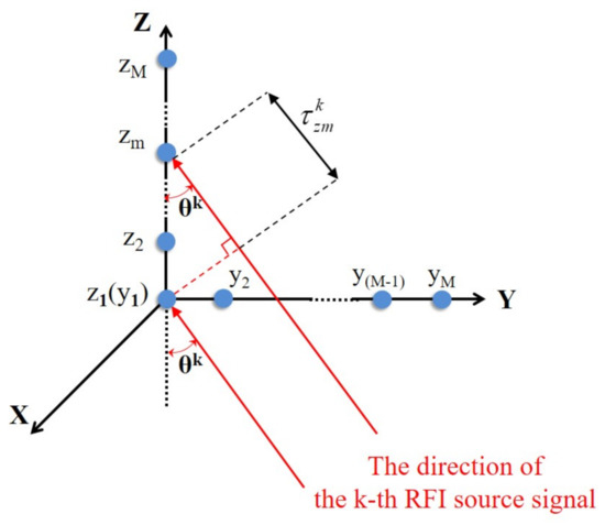
Figure 2.
The schematic diagram of the signal from the k-th RFI source being received by channel and . The time difference between the same RFI signal arriving at these two channels is .
According to the geometric relationship in Figure 2 and the definition of elevation angle in Figure 1b, the time difference of the k-th RFI signal reaching the two channels can be obtained:
where C is the light speed, is the elevation angle between the interference signal of the k-th RFI source and the array. Thus, combined with Equations (4) and (6), we can obtain:
The signal received by the M channels on the Z-axis can be expressed as a vector :
Its compact form is:
where denotes the matrix composed of interference signals from K RFI sources received by channel , and is the equivalent additive noise matrix of the M channels on the Z-axis, the steering matrix is:
In accordance with Equation (7) and the signal wavelength , can be further transformed into:
Similarly, the signals received by channel to on the Y-axis can be expressed as:
where , is the equivalent additive noise matrix of the M channels on the Y-axis. The time difference of the k-th RFI signal to channel and to channel is , it can be represented as:
Similar to , is the steering matrix of the M channels on the Y-axis, and the divergence between them is the time difference. Therefore, based on Equation (14), can be written as:
Finally, the signals of all channels form the SAR echo signal matrix :
where and . The covariance matrix of can be written as:
In addition, we define the interference-to-signal ratio (ISR) as the ratio of the power of the interference signal to the sum of the power of the real echo signal and the noise signal:
where denotes the sum of RFI signal power at each azimuth time, and denotes the sum of the real target echo signal power and the noise signal power at each azimuth time.
3. Multiple RFI Sources Geolocation Method
This section introduces the multiple RFI sources geolocation method. Firstly, the RFI detection scheme is discussed. Additionally, the minimum description length (MDL) criteria is applied to RFI source number estimation. Then, the DOA results of RFI signals at each azimuth time are calculated by performing the 2D-ESPRIT algorithm on the contaminated multi-channel SAR echo signal. Finally, on the basis of the geometric relationship between the multi-channel SAR system and RFI sources, a set of equations about the geographic location of RFI sources is established, and the results are obtained by utilizing particle swarm optimization. Figure 3 shows the process of the proposed method in summary.
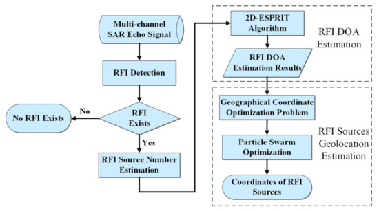
Figure 3.
Flowchart of the proposed multiple RFI sources geolocation method.
3.1. RFI Detection
In our previous research, an RFI detection method for spaceborne SAR based on deep learning technology was proposed, which has achieved good results in detecting interference and identifying its type in the interfered SAR echo. More details can be found in [19,20]. With this fast and accurate method, the existence of RFI in the echo can be effectively determined in this paper. The first step of this method is to transform the echo signal into the time-frequency domain using short-time Fourier transform (STFT) to obtain a time-frequency map. Next, a trained neural network takes this time-frequency map as input and determines whether there are RFI signals in it. If RFI exists, subsequent operations of the proposed method in this paper will then be performed.
3.2. RFI Source Number Estimation
After detecting the presence of RFI signals in the echo signal, estimating the number of interference sources is a key issue for the next steps. The minimum description length (MDL) criterion is a very effective method of estimating the number of signal sources in blind source separation based on information theory [22], which applies the minimax entropy principle and does not need to set a threshold [23]. Further, the MDL criterion can estimate the number of signal sources quite accurately under the condition of a high signal-to-noise ratio [23]. Because RFI makes the ISR of the SAR echo very high, it is extremely suitable for estimating the number of RFI sources from the contaminated multi-channel SAR echo signal based on the MDL criterion. Thus, this paper applies the MDL criterion to calculate multiple sets of echo signals of the SAR system and obtains the estimated value of the number of RFI sources. Specifically, for the estimation of the number of RFI sources, the MDL criterion searches the number of RFI signals by minimizing the following equation:
where is the number of RFI sources to be estimated, is the number of SAR channels, is the sampling number, is the likelihood function, which can be written as:
where denotes the i-th eigenvalue of the covariance matrix of SAR echo signal in Equation (17).
The procedure for estimating the number of RFI sources is to first calculate the covariance matrix of the SAR echo signal by using Equation (17) and compute the eigenvalues of . Then, the likelihood function and the MDL function are constructed according to Equations (20) and (19). Finally, all the function values of the MDL function are calculated by setting in the range of . The corresponding to the minimum of the function values is the estimated value of the number of RFI sources.
3.3. RFI DOA Estimation
RFI DOA estimation result can be obtained by applying the two-dimensional ESPRIT method to the array signal [24,25]. The ESPRIT algorithm obtains the incident angle information of the signal through the rotation invariance of the signal subspace of the array [24]. The L-shaped array, as shown in Figure 2, has two orthogonal uniform linear arrays. Each linear array can be regarded as composed of two sub-arrays, the channels on the Y-axis are divided into two sub-arrays: and . Similarly, the channels on the Z-axis are divided into and as shown in Figure 4. The special arrangement of all the channels in the L-shaped array makes the signal received by the sub-array contain the DOA information of the RFI, which can be estimated by the two-dimensional ESPRIT method. The following is the DOA estimation process.
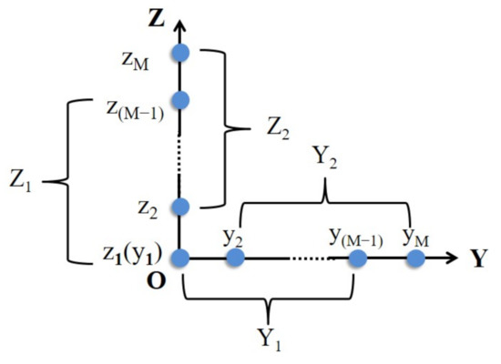
Figure 4.
Sub-arrays of the L-shaped array. Each linear array can be regarded as composed of two sub-arrays. The two sub-arrays on the Y-axis are and , the two sub-arrays on the Z-axis are and .
The Equations (10) and (13) give the signal form received by the channels on the Y-axis and the Z-axis in the L-shaped array. Further, the signals received by their sub-arrays , ,, and can be expressed as:
where and are the sub-matrices of , , and are the sub-matrices of , , , , and are the corresponding noise vectors. and have the following forms:
The relationship between Equations (22) and (23) can be written as:
Similarly, the relationship between and can be presented as:
So, according to Equations (24) and (25), Equation (21) is further derived as:
It can be easily found that and are diagonal matrices consisting of angle information, and DOA can be estimated by solving them. Then, we perform pairwise covariance operations on the signals in Equation (26) to construct the covariance matrix of these signal matrices:
where is the autocorrelation matrix of RFI signal vector, , , , and are the noise power matrices. The formulas in Equation (27) are combined into a new matrix :
When it is considered that the signal energy of RFI is much greater than the energy of echo and noise, , , , and in can be considered to be approximately zero. On this basis, the singular value decomposition of can get its signal subspace [14,25]:
where , , , and are the singular value decomposition results of , , , and , respectively, and is an invertible eigenvector matrix. The relationship between them can be expressed as:
where the relationship between and is:
Further, we can solve Equation (30) and get:
where the symbol “+” represents the Moore–Penrose pseudo-inverse of the matrix.
It is obvious that the diagonal channels of are identical to the eigenvalues of , which can be expressed as [14]:
According to Equation (31), with the assistance of performing a singular value decomposition on , its eigenvalue matrix is the estimation of . In accordance with Equation (25), the elevation angle of the k-th RFI source can be estimated:
Correspondingly, according to Equations (29) and (30), we can also get the relationship between and , and :
where is used because both and are diagonal matrices.
The solution of Equation (35) is:
Then, the estimation of is derived from the eigenvalue matrix of the singular value decomposition of :
The azimuth angle can be estimated by combining Equations (34) and (37):
It is worth mentioning that Equations (33) and (37) independently perform singular value decomposition of and , and their eigenvalues are the estimated and . However, the order of the eigenvalues and eigenvectors obtained by the two singular value decompositions may not be correspond. It means that after getting the estimation of and , we need to perform the pair-matching procedure before we can continue to use Equations (34) and (38) to obtain the DOA estimation. For this reason, the eigenvector matrices in Equations (33) and (37) may not be the same, they should be rewritten as:
where and are the eigenvectors obtained by performing singular value decomposition on and , respectively.
In the case of a low ISR, the pair-matching relationship can be obtained by constructing the cost function of the elevation angle and the azimuth angle and using an optimization algorithm to solve it [26]. However, this method will cause a large computational burden, and for RFI, the energy of the interference in the contaminated SAR signal is much greater than the energy of the echo and noise, which means the method of using optimization algorithms is unnecessary when dealing with the RFI DOA estimation problem in the situation described in this paper. Therefore, we adopt an effective method with lower computational complexity. Firstly, we use the eigenvectors to construct the following equation, and then realize the angle pairing according to the order of the maximum value [25]:
The specific approach is that after obtaining and , assume that the order of is correct, then calculate based on Equation (40), and adjust the order of according to the coordinates of the largest element in each row of , the pair-matched and are obtained in this way.
The steps of the RFI DOA estimation method used in this section are as follows.
- Step 1: In accordance with Equation (21) to get , , , and .
- Step 2: Construct with Equation (27), and perform singular value decomposition on it to get the signal subspace .
- Step 3: Calculate and with Equations (32) and (36).
- Step 4: Perform singular value decomposition on and to get and , and .
- Step 5: Perform pair-matching procedure with Equation (40).
- Step 6: Obtain and with Equations (34) and (38).
3.4. RFI Sources Geolocation Estimation
By means of applying the RFI DOA estimation algorithm in Section 3.3 to the echo signal at each azimuth time when the SAR is interfered with, the positional relationship between the interference signal of K RFI sources and the radar array at each azimuth time can be calculated.
We define represents the DOA matrix at each azimuth time, and is DOA estimation of K RFI signals at the i-th azimuth time:
Thus, at each azimuth time, a vector from the radar array to each interference source can be calculated by the DOA estimation result, its computation method approximates to Equation (41):
where represents the vector direction from the SAR system to the k-th RFI source at the i-th azimuth time calculated from the RFI DOA estimation result, and is the matrix of these estimated vector directions of all azimuth time. The schematic diagram of solving the RFI source location is shown in Figure 5.
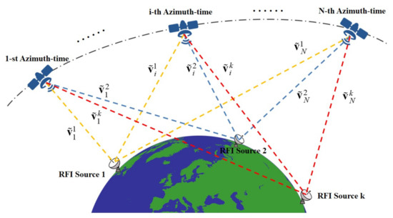
Figure 5.
Schematic diagram of RFI source location estimation. The figure shows the vector direction from the SAR system to the ground RFI sources at the 1-st, the i-th, and the N-th azimuth time obtained by using the RFI direction-of-arrival (DOA) estimation results. The dot-and-dash line represents the flight trajectory of the SAR, and the dotted line in three colors represents the estimated vector from the SAR to the three RFI sources.
We define as the spatial coordinate of the radar array at the i-th azimuth time, and denotes the spatial coordinates of the k-th RFI source. Accordingly, the vector connecting the k-th RFI source and the radar array at all azimuth time is written as:
where denotes the real vector direction from the SAR system to the k-th RFI source at the i-th azimuth time.
Obviously, if DOA estimates are accurate enough, and are parallel, which can be written as . At the i-th azimuth time, this parallel relationship can be expressed as:
Theoretically, a straight line equation like Equation (44) can be obtained at each azimuth time, and the intersection of all straight lines is the position of the RFI source, so the position of the RFI source can be solved by combining the linear equations at all azimuth time. However, the inevitable noise and systematic errors will cause DOA estimation errors, which will make the equations difficult to solve. Hence, we propose to transform this problem into an optimization problem, which is to find a point in the space coordinate system so that the sum of the distances from the point to each straight line is the smallest. It is worth noting that since almost all RFI sources are within a certain range from the ground, we can approximate that the RFI sources exist on an ellipsoid centered at the center of the earth. This will serve as a constraint for the above optimization problem In the earth-centered, earth-fixed (ECEF) coordinate system, a point on the earth can be expressed as:
where and are respectively the semi-major axis and semi-minor axis of the earth, so the constraint condition is defined as:
where represents the transformation matrix from the ENU coordinate system to the ECEF coordinate system, represents the range ratio. In this paper, we assume that the height of the RFI source does not exceed 10 km, so it should satisfy . The optimization problem for solving the coordinate position of the k-th RFI source is expressed as:
The optimization problem in Equation (47) is non-convex and needs to be solved in its nonlinear constraints, the particle swarm optimization is applied to solve it. As a method with the ability to solve non-convex problems and global search capabilities, the PSO algorithm is easy to be implemented and the computational cost is low in memory requirements [27]. It is also a derivative-free method that can achieve convergence rapidly. Not only that, it can find a good solution in a complex search range based on the experience of particle swarms [27]. It first randomly initializes a group of particles, and then continuously searches for suitable function values in the domain. In this process, these particles share information, which enables them to constantly adjust their own optimization direction and finally find the optimal solution in the complex search space [27]. In the solution process, we define the size of the particle swarm as and use the optimization function and constraint conditions in Equation (47) as the fitness function and search range of the PSO algorithm. As mentioned above, the solution of this optimization problem is a three-dimensional vector, so during the t-th iteration the position of the j-th particle in the search space can be represented by a three-dimensional vector , and its velocity is . The shared information of the particle swarm during the t-th iteration calculation is: a) Individual optimal position: the best position that the j-th particle has ever been to is ; (b) Group optimal position: the global best position of the group discovered so far is expressed as . The position of each particle in any iteration represents a possible solution. After each iteration is completed, fitness is used to select and update the individual optimal position and the group optimal position:
where denotes the inertia weight, and are the cognitive and group scaling parameters and their value range is , and are two random values selected in the t-th iteration within the range . According to Equations (47) and (48), the solver of the position optimization problem can be constructed.
In summary, the procedure of the RFI sources geolocation estimation method used in this section can be summarized as follow. Firstly, according to the spatial coordinate at the i-th azimuth time of the radar array, the vector from the k-th RFI source to the radar array and the transformation matrix , the optimization problem in Equation(47) can be constructed. Then, the PSO algorithm shown in Figure 6 is applied to solve it.
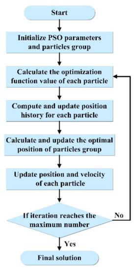
Figure 6.
Flowchart of the particle swarm optimization (PSO) algorithm.
4. Simulation Experiments and Results
4.1. System Establishment and Parameter Setting
In Section 3, the multiple RFI sources geolocation method based on the 2D-ESPRIT and PSO algorithm has been discussed. In this section, the simulation results obtained by processing on the simulated data using the proposed method are presented. First, we establish a spaceborne multi-channel SAR system that may be affected by single or multiple RFI source. Next, on the basis of this system, the RFI transmitted from multiple different spatial locations and existing at the same time is simulated, and the contaminated echo signals received by the SAR under these conditions are obtained. The key parameters of SAR system in the simulation works are shown in Table 1.

Table 1.
Synthetic aperture radar (SAR) system parameters.
For the echo signal, we take the pixel value of a real SAR image as the backscattering coefficient of the scene, in accordance with the radar and antenna parameters set in Table 1, and the relative position of SAR and the scene set as Figure 1a, the scene echo signal is calculated pulse by pulse. We have successfully applied this method in previous studies to generate echo signals [17,19,20].
For RFI sources, we define that RFI sources are independent of each other, and each RFI source is located at a place not lower than the surface of the earth, the form of interference signals emitted by them is in accordance with Equation (2). In order to fully verify the effectiveness of the proposed method, various simulation experiments are conducted. In each simulation experiment, the emission signal of the interference source is randomly generated according to Equation (2). The specific method is to first randomly generate the characteristic parameters of the signal within a certain range and then substitute these parameters into the equation to obtain the signal. In this way, the interference signal of each simulation can conform to the RFI signal characteristics and independent characteristics. The range and approach of randomly generating RFI signal parameters are shown in Table 2. Based on the above system parameters and interference parameters, a spaceborne SAR simulation system interfered with by RFI sources can be established.
Table 2.
The range and approach of randomly generating RFI signal parameters.
Further, pursuant to the number of RFI sources and the type of interference signal, we design three situations when the SAR system is jammed:
- Case 1. A single RFI source.
- Case 2. Multiple RFI sources of the same interference type.
- Case 3. Multiple RFI sources of mixed types.
With the established SAR system, we simulate the SAR echo signals with different interference -to-signal ratios in these three conditions and use them as experimental data.
4.2. Simulation Experiments and Results
According to the parameters in Table 1 and Table 2, the contaminated echo signals are simulated. At each azimuth time, the interference signal of all RFI sources, the real target echo signal, and the noise signal constitute the echo signal of the SAR system according to Equation (1). Figure 7 shows the time-domain and frequency-domain forms of the demodulated SAR echo signals interfered by the three types of RFI signals.
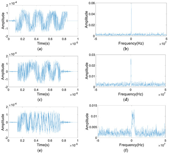
Figure 7.
Time-domain and frequency-domain form of the contaminated SAR signal: (a) time-domain form of echo signal contaminated by radio frequency noise interference (RFNI); (b) frequency-domain form of (a); (c) time-domain form of echo signal contaminated by narrowband linear frequency modulated interference (NBLFMI); (d) frequency-domain form of (c); (e) time-domain form of echo signal contaminated by wideband linear frequency modulated interference (WBLFMI); (f) frequency-domain form of (e).
The performance of the two-dimensional DOA algorithm is proved via the simulation experiments. Based on the obtained echo signal, we adopt the Monte Carlo simulation method for the DOA estimation method proposed in Section 3.3, and for each case, the number of Monte Carlo trials is 1000. Generally, the root mean square error (RMSE) of the angle estimation result is defined as an index to evaluate the performance of the two-dimensional DOA algorithm:
In Case 1, the RFI source is located at , and it is expressed in meters. In each experiment, we set the transmit power of the RFI source and set it to transmit one of the three interference signals, and then use the two-dimensional DOA method to process the echo signal and estimate the arrival angle. Figure 8 shows the DOA estimation error when the RFI source transmits three kinds of interference signals separately. Each point in Figure 8 represents the error between the estimated DOA and the true DOA in azimuth and elevation .
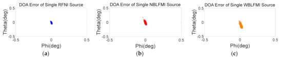
Figure 8.
Angle estimation accuracy for Case 1 where a single RFI source transmits one of the three types of RFI in one experiment. The horizontal axis represents the error of the azimuth angle, and the vertical axis represents the error of the elevation angle in these figures: (a) DOA error of single RFNI source; (b) DOA error of single NBLFMI source; (c) DOA error of single WBLFMI source.
For each type of RFI, we gradually increase the transmit power of the RFI source, which will make the ISR of the echo signal increase accordingly. Then, the RMSE of the DOA estimation under each ISR is calculated and recorded. The RMSE of the angle estimation for this case can be calculated by substituting the DOA estimation result into Equation (49). The RMSE of angle estimation when interference transmitting power gradually increases is shown in Figure 9.
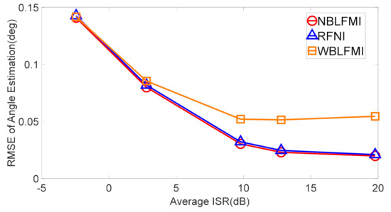
Figure 9.
The root mean square error (RMSE) of angle estimation under different interference-to-signal ratio (ISR) for Case 1.
In Case 2, three RFI sources of the same type are set in the system, and their geolocation coordinates in the ENU coordinate system respectively are , , and , all these coordinates are expressed in meters. As ISR is 10 dB, the angle estimation results are shown in Figure 10. The RMSE in this case is shown in Figure 11. Similar to Figure 8, each point in Figure 10 represents the error between the estimated DOA and the true DOA in azimuth and elevation .
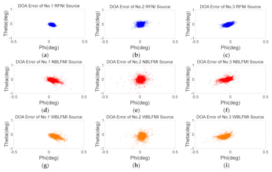
Figure 10.
Angle estimation accuracy for Case 2 where three RFI sources transmit the same type of interference simultaneously. The horizontal axis represents the error of the azimuth angle, and the vertical axis represents the error of the elevation angle in these figures: (a–c) DOA error of RFNI sources; (d–f) DOA error of NBLFMI sources; (g–i) DOA error of WBLFMI sources. (a,d,g) RFI source locates at (b,e,h) RFI source locates at ; (c,f,i) RFI source locates at .
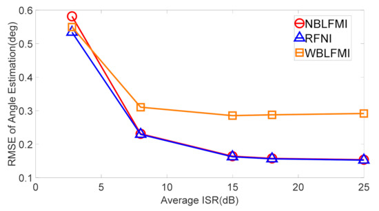
Figure 11.
RMSE of angle estimation for Case 2.
In Case 3, the number of RFI sources and geographic coordinates are the same as Case 2. As ISR is 10 dB, the angle estimation result is shown in Figure 12. The RMSE in this case and Case 2 are integrated and shown in Figure 13.
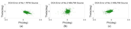
Figure 12.
Angle estimation result for Case 3 where three RFI sources transmit the different types of interference simultaneously. The horizontal axis represents the error of the azimuth angle, and the vertical axis represents the error of the elevation angle in these figures. (a) RFI source locates at ; (b) RFI source locates at ; (c) RFI source locates at .
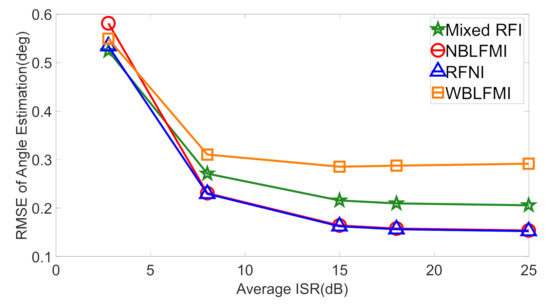
Figure 13.
RMSE of angle estimation for Case 2 and Case 3.
Then, we verify the performance of the PSO algorithm to calculate the spatial coordinates of the RFI source. The parameter selection refers to the principle of parameter setting in [28], equal to 0.5, and both equal to 2.0. Figure 14 indicates the process of using the PSO algorithm to solve the optimization problem in Equation (47).
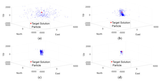
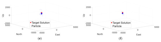
Figure 14.
Process of PSO algorithm: (a) Iterations = 1; (b) Iterations = 10; (c) Iterations = 50; (d) Iterations = 100; (e) Iterations = 120; (f) Iterations = 161.
Similarly, the RMSE of the estimated location and the true location can be used to illustrate the localization accuracy:
When the transmission power gradually increases, the RMSE of the estimated location in the three cases is shown in Figure 15.
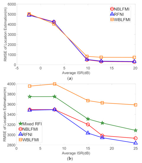
Figure 15.
RMSE of location estimation for multiple RFI sources: (a) RMSE of geolocation estimation for Case 1; (b) RMSE of geolocation estimation for Case 2 and 3.
In order to evaluate the validity of the location estimation result obtained using the proposed method, digital beamforming (DBF) is used to mitigate the RFI in the echo signal with this result as the input, and the imaging results of the suppressed signal get to illustrate the effectiveness. The RFI suppression method aligns the notch direction of the beamforming pattern with the direction of the RFI source to reduce the energy of the RFI in the echo signal [9,10]. In this paper, we use the DBF algorithm described in Reference [9]. Specifically, the estimated RFI source geographic location is utilized to calculate the elevation and azimuth angles of the RFI signal reaching the channel array at each azimuth time, and the optimal problem for RFI suppression is established according to the linearly constrained minimum variance (LCMV) method in DBF on the basis of the estimated angles [9]. The beamforming pattern weight is acquired by solving the optimization problem and the signal after RFI suppressing can be get by multiplying this weight with the channel signal , which is given as [9]:
Combined with the results of Figure 8, Figure 10 and Figure 12, we respectively apply the estimated RFI source location results of Cases 1–3 to the DBF algorithm to obtain the beamforming pattern weights in the elevation and azimuth directions at each azimuth time. Figure 16 shows the beamforming pattern weights calculated by using the elevation and azimuth estimation results at half of the azimuth time for Cases 1–3. In Figure 16a,b, are the result of the RFI type being RFNI in Case 1, (c) and (d) are the result of the RFI type being NBLFMI in Case 2, and (e) and (f) are the result in Case 3. These figures show the weights of the beamforming pattern at various angles, and the red dashed line represents the direction of interference, and the black dashed line represents the direction of the connection between the center of the scene and the array. As shown in Equation (51), the signal in the interference direction will be weakened by multiplying these weights with the signal matrix, which achieves interference suppression.
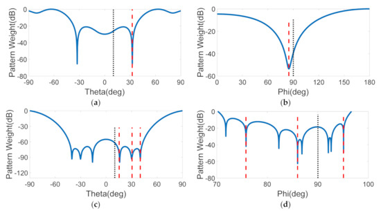
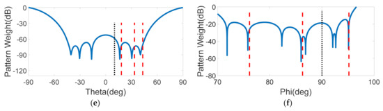
Figure 16.
Beamforming pattern weights calculated by using the elevation and azimuth estimation results at half of the azimuth time for Cases 1–3: (a) and (b) are the result of the RFI type being RFNI in Case 1; (c) and (d) are the result of the RFI type being NBLFMI in Case 2; (e) and (f) are the result of Case 3.
Next, the BP imaging algorithm is applied to the signal after interference suppression to get the image results in Figure 17. Figure 17a shows the SAR image of the RFI-free echo signal. Then, the BP imaging algorithm is used to process the echo signals in Case 2 that are interfered by three RFI sources of the same type to obtain contaminated SAR images in Figure 17b,d,f. They are interfered by RFNI, NBLFMI, and WBLFMI, respectively. Figure 17c,e,g represents the imaging results after interference suppression on the signals in (b), (d), and (f). Likewise, (h) and (i) are the images for Case 3. It can be seen from the interfered images that when subjected to different types of RFI, the interference in the image is different. For the images after interference suppression, RFI is greatly suppressed, but the quality of these images is not as good as the RFI-free images. Therefore, the ISR of the signal before and after interference suppression can be used to show the degree of RFI suppression.
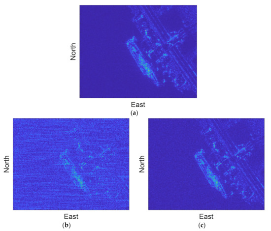
Figure 17.
SAR images obtained by applied the imaging algorithm to the echo signals: (a) RFI-free image; (b,d,f) are contaminated images for Case 2; (c,e,g) are RFI suppressed images of (b,d,f); (h,i) are contaminated and RFI suppressed images for Case 3.
The ISRs before and after interference suppression are calculated after obtaining the RFI suppressed signal. The ISR before interference suppression is obtained by Equation (18), the ISR after interference suppression and the improvement of ISR of the signal can be written as:
Table 3 shows the improvement of ISR after applying the above interference suppression methods to the signals in Figure 8, Figure 10 and Figure 12, respectively. For Case 1, because of the higher location accuracy of the RFI source, the improvement of the signal ISR is better than other situations. In Case 2, the location accuracy is the worst for the interference type WBLFMI, which also leads to the smallest improvement in its ISR. The improvement of Case 3 is better than that of WBLFMI in Case 2, which is also consistent with the result of location accuracy.
Table 3.
The range and approach of randomly generating RFI signal parameters.
5. Discussion
In Section 4, by setting the system and interference parameters, we simulate and get the SAR echo signals contaminated by the three types of RFI, whose time domain and frequency domain forms are shown in Figure 7. Furthermore, a series of experiments are set up to discuss the performance of the 2-D ESPRIT method and the PSO algorithm under different type RFI sources and ISR conditions.
For the 2-D ESPRIT method, Figure 8, Figure 10 and Figure 12 show the DOA error between the estimation result and the true value at each azimuth time. It can be seen that the estimation error of does not exceed , and the estimation error of does not exceed , and most of the estimation errors are small. This demonstrates that the method has a good performance in the DOA estimation of RFI sources. Comparing these three figures, we can further find that the performance of the method varies under different RFI types and ISR conditions, which can be more intuitively reflected in the RMSE results of the angle estimation. Figure 9, Figure 11 and Figure 13 show that with the gradual increase of ISR, the RMSE of the angle estimation in the three cases decrease, which illustrates that the proposed method can achieve high angle measurement accuracy when the ISR is large. It can be seen from Section 3 that the presence of noise and echo signals will make the calculation result of Equation (32) contain components that are not related to RFI, which will cause errors in the azimuth and elevation angles estimated by Equations (34) and (38). And the error increases as the ISR becomes smaller, which is consistent with the above experimental results. Meanwhile, it can be seen in the three figures that the method has different angle measurement capabilities for the three types of interference. It has the highest measurement accuracy for RFNI, followed by NBLFMI and WBLFMI. Because when the bandwidth of the RFI gradually increases, the error between the wavelength used in Equations (34) and (38) and the true wavelength of RFI increases, which will also bring error in angle measurement. In addition, we can see from the comparison between Figure 9 and Figure 11 that the optimal value of RMSE estimated for the angle of RFNI in Case 1 is , while in Case 2, the value is , which indicates that when the number of channels is the same, the DOA estimation accuracy of this method for a single RFI source is better than that of multiple RFI sources.
For the method of using DOA estimation results and PSO algorithm to estimate RFI source position coordinates, experiments also show the effectiveness of it. Illustrated in Figure 14, the particle swarm is gradually optimized to the target solution point as the iteration continues. However, the value obtained after the convergence of the PSO algorithm is slightly different from the true value, which is caused by the DOA estimation error and the random search solution process. Figure 14 also shows that the method can calculate the coordinate estimation value of the RFI source in the three cases. For Case 1, the optimal value of the RMSE of the position estimation is 284.54 m, while in Case 2 and Case 3, the value is respectively 2836.02 and 308.632 m. This proves that under the conditions of the simulation parameters set in this paper, the minimum coordinate estimation error of a single RFI source is 284.54 m, and the minimum coordinate estimation error of multiple RFI sources is 2836.02 m, so the coordinate estimation of a single RFI source is more accurate than that of multiple RFI sources. Likewise, similar to the DOA estimation result, the RMSE of the geographical location estimation in the three cases decreases with ISR increasing. Additionally, this method also has better performance for RFI signals with a narrow bandwidth. It can be proven that the location error is highly consistent with the DOA estimation error in the proposed method.
In the evaluation part, the estimated RFI source location and the DBF algorithm are utilized to suppress the RFI signal. The results in Figure 16 indicate that the obtained beamforming pattern will form a notch in a given interference direction to perform interference suppression. Although the location estimation result with errors will deviate the notch direction from the real RFI direction, the beamforming pattern also has a strong weakening effect on incoming signals within a certain error range, which means that these errors will not have a great impact on the use of the DBF algorithm to suppress interference. The results in Figure 17 and Table 3 illustrate that the RFI source location coordinates estimated by the proposed method are useful for interference suppression. They also show that the location estimation error has an impact on the interference suppression effect, but this effect is small and tolerable.
In summary, this proposed approach in this paper can estimate the geographic coordinates of the RFI source and the estimation error is acceptable.
6. Conclusions
In this paper, we have proposed a novel method for the location of multiple independent RFI sources based on the two-dimensional ESPRIT and PSO algorithm. First of all, the multi-channel spaceborne SAR echo signal model containing interference signals is established. In addition, RFI detection and interference source number estimation are performed. Furthermore, we take into account the spatial distribution characteristics of SAR signals and propose to apply the 2D-ESPRIT algorithm to the echo signal processing of the multi-channel SAR. Next, the DOA of the interference signal at each azimuth time can be achieved, which are applied to establish a set of nonlinear equations containing the coordinates of RFI sources. Finally, relying on the particle swarm optimization algorithm, we can solve these equations to obtain the geographic coordinates of RFI sources. The results obtained from the simulation experiments indicate that the proposed method provides good performance in estimating the RFI angle of arrival and geographic location. In future work, real SAR signals interfered by RFI will be used to verify the performance of this method.
Author Contributions
Conceptualization, J.Y., B.S. and Y.J.; Formal analysis, J.Y.; Investigation, J.Y.; Methodology, J.Y. and Y.J.; Resources, J.L., B.S. and L.X.; Supervision, J.L. and B.S.; Writing—original draft preparation, J.Y.; Writing—review and editing, B.S. All authors have read and agreed to the published version of the manuscript.
Funding
This research was funded by National Natural Science Foundation of China under Grant 62071022 and 61801294.
Institutional Review Board Statement
Not applicable.
Informed Consent Statement
Not applicable.
Data Availability Statement
Not applicable.
Conflicts of Interest
The authors declare no conflict of interest.
References
- Natsuaki, R.; Motohka, T.; Watanabe, M.; Shimada, M.; Suzuki, S. An Autocorrelation-Based Radio Frequency Interference Detection and Removal Method in Azimuth-Frequency Domain for SAR Image. IEEE J. Sel. Top. Appl. Earth Obs. Remote Sens. 2017, 10, 1–16. [Google Scholar] [CrossRef]
- Tao, M.; Zhou, F.; Zhang, Z. Wideband Interference Mitigation in High-Resolution Airborne Synthetic Aperture Radar Data. IEEE Trans. Geosci. Remote Sens. 2015, 54, 74–87. [Google Scholar] [CrossRef]
- Yang, Z.; Du, W.; Liu, Z.; Liao, G. WBI Suppression for SAR Using Iterative Adaptive Method. IEEE J. Sel. Top. Appl. Earth Obs. Remote Sens. 2017, 9, 1008–1014. [Google Scholar] [CrossRef]
- Tao, M.; Zhou, F.; Liu, J.; Liu, Y.; Zhang, Z.; Bao, Z. Narrow-Band Interference Mitigation for SAR Using Independent Subspace Analysis. IEEE Trans. Geosci. Remote Sens. 2014, 52, 5289–5301. [Google Scholar]
- Zhou, F.; Tao, M. Research on Methods for Narrow-Band Interference Suppression in Synthetic Aperture Radar Data. IEEE J. Sel. Top. Appl. Earth Obs. Remote Sens. 2017, 8, 3476–3485. [Google Scholar] [CrossRef]
- Zhou, F.; Tao, M.; Bai, X.; Liu, J. Narrow-Band Interference Suppression for SAR Based on Independent Component Analysis. IEEE Trans. Geosci. Remote Sens. 2013, 51, 4952–4960. [Google Scholar] [CrossRef]
- Meyer, F.J.; Nicoll, J.B.; Doulgeris, A.P. Correction and Characterization of Radio Frequency Interference Signatures in L-Band Synthetic Aperture Radar Data. IEEE Trans. Geosci. Remote Sens. 2013, 51, 4961–4972. [Google Scholar] [CrossRef]
- Zhang, S.; Xing, M.; Guo, R.; Zhang, L.; Bao, Z. Interference suppression algorithm for SAR based on time–frequency transform. IEEE Trans. Geosci. Remote Sens. 2011, 49, 3765–3779. [Google Scholar] [CrossRef]
- Rosenberg, L.; Gray, D.A. Constrained Fast-Time STAP for Interference Suppression in Multichannel SAR. IEEE Trans. Aerosp. Electron. Syst. 2013, 49, 1792–1805. [Google Scholar] [CrossRef]
- Bollian, T.; Osmanoglu, B.; Rincon, R.; Lee, S.K.; Fatoyinbo, T. Adaptive Antenna Pattern Notching of Interference in Synthetic Aperture Radar Data Using Digital Beamforming. Remote Sens. 2019, 11, 1346. [Google Scholar] [CrossRef]
- Bollian, T.; Osmanoglu, B.; Rincon, R.F.; Lee, S.K.; Fatoyinbo, T.E. Detection and Geolocation of P-Band Radio Frequency Interference Using EcoSAR. IEEE J. Sel. Top. Appl. Earth Obs. Remote Sens. 2018, 11, 1–9. [Google Scholar] [CrossRef]
- Li, J.; Hu, F.; He, F.; Wu, L. High-Resolution RFI Localization Using Covariance Matrix Augmentation in Synthetic Aperture Interferometric Radiometry. IEEE Trans. Geosci. Remote Sens. 2017, 56, 1186–1198. [Google Scholar] [CrossRef]
- Hu, F.; Wu, L.; Li, J.; Peng, X.; Zhu, D.; Cheng, Y. RFI localization in synthetic aperture interferometric radiometers based on sparse Bayesian inference. Int. J. Remote Sens. 2017, 38, 5502–5523. [Google Scholar] [CrossRef]
- Gu, J.F.; Zhu, W.P.; Swamy, M.N.S. Joint 2-D DOA estimation via sparse L-shaped array. IEEE Trans. Signal Process. 2015, 63, 1171–1182. [Google Scholar] [CrossRef]
- Dong, Y.Y.; Dong, C.X.; Liu, W.; Chen, H.; Zhao, G.Q. 2-D DOA estimation for L-shaped array with array aperture and snapshots extension techniques. IEEE Signal Process. Lett. 2017, 24, 495–499. [Google Scholar] [CrossRef]
- Tao, M.; Su, J.; Huang, Y.; Wang, L. Mitigation of Radio Frequency Interference in Synthetic Aperture Radar Data: Current Status and Future Trends. Remote Sens. 2019, 11, 2438. [Google Scholar] [CrossRef]
- Yu, J.; Li, J.; Sun, B.; Chen, J.; Li, C.; Li, W.; Xu, L. Single RFI Localization Based on Conjugate Cross-Correlation of Dual-Channel SAR Signals. In Proceedings of the IGARSS 2019–2019 IEEE International Geoscience and Remote Sensing Symposium, Yokohama, Japan, 28 July–2 August 2019. [Google Scholar]
- Liang, J.; Liu, D. Joint Elevation and Azimuth Direction Finding Using L-Shaped Array. IEEE Trans. Antennas Propag. 2010, 58, 2136–2141. [Google Scholar] [CrossRef]
- Yu, J.; Li, J.; Sun, B.; Chen, J.; Li, C. Multiclass Radio Frequency Interference Detection and Suppression for SAR Based on the Single Shot MultiBox Detector. Sensors 2018, 18, 4034. [Google Scholar] [CrossRef] [PubMed]
- Junfei, Y.; Jingwen, L.; Bing, S.; Yuming, J. Barrage Jamming Detection and Classification Based on Convolutional Neural Network for Synthetic Aperture Radar. In Proceedings of the IGARSS 2018—2018 IEEE International Geoscience and Remote Sensing Symposium, Valencia, Spain, 22–27 July 2018. [Google Scholar]
- Meyer, F.J.; Nicoll, J.B.; Doulgeris, A.P. Characterization and extent of randomly-changing radio frequency interference in ALOS PALSAR data. In Proceedings of the 2011 IEEE International Geoscience and Remote Sensing Symposium, Vancouver, BC, Canada, 24–29 July 2011; pp. 2448–2451. [Google Scholar]
- Wax, M.; Kailath, T. Detection of signals by information theoretic criteria. IEEE Trans. Acoust. Speech Signal Process. 1985, 33, 387–392. [Google Scholar] [CrossRef]
- Li, Y.O.; Adalı, T.; Calhoun, V.D. Estimating the number of independent components for functional magnetic resonance imaging data. Hum. Brain Mapp. 2007, 28, 1251–1266. [Google Scholar] [CrossRef] [PubMed]
- Tayem, N.; Majeed, K.; Hussain, A.A. Two-Dimensional DOA Estimation Using Cross-Correlation Matrix with L-Shaped Array. IEEE Antennas Wirel. Propag. Lett. 2016, 15, 1077–1080. [Google Scholar] [CrossRef]
- Cheng, Q.; Zhao, Y.; Yang, J. Improvement of 2-D DOA estimation based on L-shaped array. In Proceedings of the ISAPE2012, Xi’an, China, 22–26 October 2012. [Google Scholar]
- Yang, X.; Zheng, Z.; Ko, C.C.; Zhong, L. Low-complexity 2D parameter estimation of coherently distributed noncircular signals using modified propagator. Multidimens. Syst. Signal Process. 2017, 28, 407–426. [Google Scholar] [CrossRef]
- Clerc, M.; Kennedy, J. The particle swarm—Explosion, stability, and convergence in a multidimensional complex space. IEEE Trans. Evol. Comput. 2002, 6, 58–73. [Google Scholar] [CrossRef]
- Suganthan, P.N. Particle swarm optimiser with neighbourhood operator. In Proceedings of the 1999 Congress on Evolutionary Computation-CEC99, Washington, DC, USA, 6–9 July 1999; pp. 1958–1962. [Google Scholar]
Publisher’s Note: MDPI stays neutral with regard to jurisdictional claims in published maps and institutional affiliations. |
© 2021 by the authors. Licensee MDPI, Basel, Switzerland. This article is an open access article distributed under the terms and conditions of the Creative Commons Attribution (CC BY) license (http://creativecommons.org/licenses/by/4.0/).