Forest Fuel Loads Estimation from Landsat ETM+ and ALOS PALSAR Data

Abstract

Fuel load is the key factor driving fire ignition, spread and intensity. The current literature reports the light detection and ranging (LiDAR), optical and airborne synthetic aperture radar (SAR) data for fuel load estimation, but the optical and SAR data are generally individually explored. Optical and SAR data are expected to be sensitive to different types of fuel loads because of their different imaging mechanisms. Optical data mainly captures the characteristics of leaf and forest canopy, while the latter is more sensitive to forest vertical structures due to its strong penetrability. This study aims to explore the performance of Landsat Enhanced Thematic Mapper Plus (ETM+) and Advanced Land Observing Satellite (ALOS) Phased Arrayed L-band Synthetic Aperture Radar (PALSAR) data as well as their combination on estimating three different types of fuel load—stem fuel load (SFL), branch fuel load (BFL) and foliage fuel load (FFL). We first analyzed the correlation between the three types of fuel load and optical and SAR data. Then, the partial least squares regression (PLSR) was used to build the fuel load estimation models based on the fuel load measurements from Vindeln, Sweden, and variables derived from optical and SAR data. Based on the leave-one-out cross-validation (LOOCV) method, results show that L-band SAR data performed well on all three types of fuel load (R² = 0.72, 0.70, 0.72). The optical data performed best for FFL estimation (R² = 0.66), followed by BFL (R² = 0.56) and SFL (R² = 0.37). Further improvements were found for the SFL, BFL and FFL estimation when integrating optical and SAR data (R² = 0.76, 0.81, 0.82), highlighting the importance of data selection and combination for fuel load estimation.

1. Introduction

Wildfires are disturbances that exist in various ecosystems, which play an important role in the formation and succession of ecosystems [1]. Humankind benefited from fires for millennia, since wildfires help to control pests and contribute to the regulation of biogeochemical cycles which benefit plants in adapting to novel climates, thus providing a range of goods and services (food, fiber, pollination, tourism, hunting) to us [2]. However, with global climate change and urban expansion, the negative effects of wildfires increased [3]. Wildfires are even increasingly recognized as a natural hazard that can cause significant social, economic, and environmental harms [4]. Besides, global meteorological studies show that fire seasons worldwide are lengthening, and the fire weather is becoming more extreme [5,6,7]. Therefore, early fire prevention and extinction are urgent. Fuel load (FL) is the key factor for the assessment of fire flame length [8,9], fuel consumption [10] and fire severity [11], which is also an indispensable input of fire behavior models [12,13,14]. Generally, FL refers to the dry weight per unit area of all combustible materials [15,16]. Fires in the natural environment are always caused by extremely high-temperature conditions such as lightning strikes [17,18]. In this case, the fuel loads that support lightning fires in the forest include foliage fuel load (FFL), branch fuel load (BFL) and stem fuel load (SFL) [19,20,21], which are defined as the dry weight of foliage, branch and stem per unit area, respectively. Among which, canopy fuel load (i.e., the sum of BFL and FFL) is more important than SFL in fire warning as it contains the main potential energy source supporting crown fires [14] which have a faster spreading rate, stronger burning intensity, and more severe and lasting effects than surface fires [22,23]. Therefore, accurately predicting the spatiotemporal continuous distribution of above-ground forest fuel loads (i.e., SFL, BFL and FFL) will not only assist fire managers in removing excess FLs in advance to avoid large-scale fires but also provides decision support for firefighters in removing isolation zones and judging the spread of fire when fires occur [13].

Traditional ground measurement of FL estimates usually use statistical formulas to establish relationships between numerous destructive field measurements and forest stand structure parameters (e.g., height, diameter at breast height (DBH), etc.) or collect coarse resolution ground data (i.e., sparse destructive fuel load samples) combined with an interpolation method to obtain a relatively fine fuel load distribution, but both of them are time-consuming, labor-intensive and introduce greater uncertainty into the fire risk model [14,24,25].

As a large-scale and long-term earth observation technology, remote sensing provides a favorable chance to create quantitative descriptions of FLs [13,26]. There are studies on the quantitative inversion of fuel load mainly employing light detection and ranging (LiDAR) data [27,28,29,30], multispectral optical data [13,22,31,32] and synthetic aperture radar (SAR) [33].

LiDAR is an active mode of operation that emits a laser beam to receive backscattered or reflected light from the target [34,35]. Compared to other remote sensing data, LiDAR can provide three-dimensional information of forest structure and spatial characteristics of surface fuel depth and coverage, topography and canopy density, especially in forest surface fuel load estimation [27]. Additionally, strong correlations were found between LiDAR height distribution and canopy fuel parameters, among which the determined coefficient (R²) with canopy fuel loads reached 0.86 [12]. However, LiDAR has limitations for the wall-to-wall coverage of large-scales or engineering applications since it is costly [36,37].

The multispectral optical remote sensing captures the spectral reflectance forest canopy at a two-dimensional distribution of fuel load, which can describe the leaf biochemical properties and standing woody material geometrical features [38]. The primary method of fuel load estimation using optical data is to classify vegetation types through spectral bands or vegetation indices (VIs) first, then predict fuel load with fire history information [13]. Moreover, for high spatial resolution optical data (e.g., Quickbird, IKONOS), some researchers used image texture information such as the shadow fraction of the tree crown, and then combining regression analysis to estimate canopy fuel load [16,31]. Nevertheless, optical data can only reflect some information about foliage distributed at the top of the canopy but lack the vertical structure information due to its limited penetration.

Synthetic aperture radar (SAR), represented by active microwave with polarimetric information without being affected by weather conditions, has been applied to many earth surface variable observations [39,40]. Spaceborne SAR sensors transmit various wavelength bands including X-, C- and L-band which have different capabilities of penetration, e.g., the C-band can penetrate foliage, but will be dispersed by small branches while the longer-wavelength L-band signal interacts with thick branches and trunks [41,42,43,44]. Within this context, SAR, especially those with long wavelengths, have great potential in forest fuel loads estimation. Saatchi et al. combined the airborne L-band and P-band HV polarizations to estimate the canopy fuel load empirically, and R² is greater than 0.7 [33]. However, airborne SAR is costly which limits its potential to monitor fuel loads on a large region or even global scale.

To date, the potential of optical and SAR data, as well as their combination for fuel load estimation, still lacks exploration. Optical and SAR data have different advantages in ground observation. The former is closely related to the biochemical characteristics of foliage but is less sensitive to the vertical structure information of the branches, while the latter can penetrate foliage to obtain branch and stem information. Within this context, the Landsat ETM+ optical data and the Advanced Land Observing Satellite (ALOS) PALSAR L-band SAR data were integrated to estimate the above-ground forest fuel loads in Vindeln, Sweden. We evaluated the performances of optical and SAR data as well as their combination on FL estimation individually to explore the feasibility of spectral band and backscattering information, which provided references for subsequent data selection of FLs estimation, and further increased the possibility of large-scale high-precision fire risk early warning.

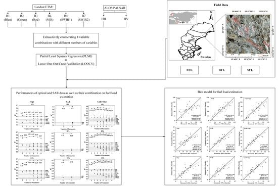
2. Materials and Methods

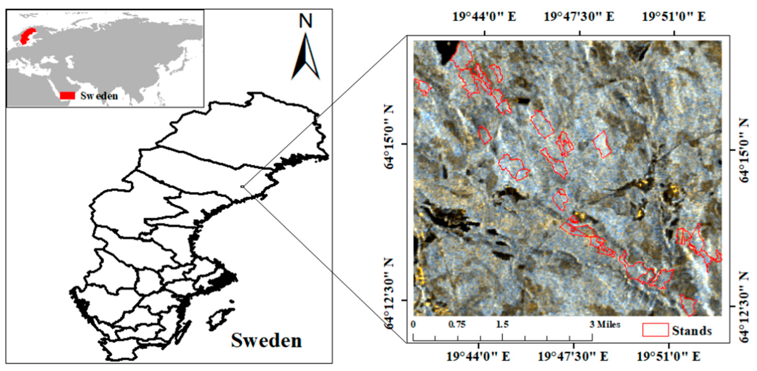
2.1. StudyAarea and Field Measurements

The study area is located in the Vindeln municipality, Västerbotten province of northern Sweden about 50 km northwest of Umeå (64°14’N, 19°46’E) which is covered by mixed coniferous forest. The region is considered to be in between a coastal and an inland climate. The mean annual temperature is 1.42 °C and the mean annual precipitation is 600 mm, of which approximately 50% is snowfall. The landscape is rugged, with a 239-meter difference in topography [45].

The field data of SFL, BFL and FFL were obtained from the BioSAR 2008 dataset, which was expressed as forest stands and measured in October 2008. The data are available in the European Space Agency (ESA) Earth Observation campaigns (http://eopi.esa.int last access 22 February 2021).

A total of 31 stands were investigated whose size varied between 2.4 and 26.3 ha. The trees which had a DBH (diameter at breast height) greater than 4 cm were measured and recorded. A number of 15 sample trees were randomly selected (selected with a probability proportional to their basal area) per stand on average to measure their height and age. These stands are dominated by evergreen coniferous forest including Scots pine and Norway spruce. The fuel load is calculated based on the allometric equations and field survey for different tree species [46]. More details about the field data can be found in [47]. Two stands were found located near bare land, which would bring errors to the analysis. Therefore, we excluded these two stands, and finally kept 29 forest stands, shown as the red border polygon in Figure 1.

2.2. Satellite Data

The ALOS (Advanced Land Observing Satellite) PALSAR provides long-wavelength (23.6 cm) data in the L-band [48]. Large-scale PALSAR datasets compiling the ortho-rectified and slope-corrected SAR long-strip images were produced by a mosaic algorithm, providing HH and HV polarizations at a spatial resolution of 25 m [49]. In this study, we used the mosaic product mentioned above in the year 2008, downloaded from Google Earth Engine (GEE) [50]. The radar signal of mosaic data can be transformed into either radar backscattering coefficients or gamma naught (${\mathsf{\gamma }}^0$) values. Here, we converted the digital numbers into ${\mathsf{\gamma }}^0$ using Equation (1), because it can better capture the structure and distribution characteristics of the forest [51].

$${\mathsf{\gamma }}^0\left(\mathrm{dB}\right){=10\times \log }_{10}\left({\mathrm{DN}}^2\right)-83$$

(1)

where DN is the digital number and ${\mathsf{\gamma }}^0$ is in the dB unit.

All pixel in each forest stand was extracted and the averaged ${\mathsf{\gamma }}^0$ was used as the SAR observed value.

The surface reflectance data of Landsat 7 ETM+ with a spatial resolution of 30 m were used in this study. In order to match the date of in situ measurements, a preprocessed Landsat 7 ETM+ (7 October 2008) product was selected and downloaded from GEE. However, since the Landsat 7 sensor was damaged in 2003 [52], part of the stands were affected by the lack of data due to scan-line-off strips in this image. A total of 28 stands were found with more than 50% valid observations (the ratio was calculated as the stands’ valid number of pixels divided by the total number of pixels) and only one stand had 44.36% valid observations. For the stands without the influence of strips, all pixel was extracted and averaged. For the stands partly affected by strips, we only used the pixels out of the strips to calculate the averaged reflectance. All satellite data used in this study are listed in

Table 1. Detail information about variables used for fuel load modeling. ALOS: Advanced Land Observing Satellite.

Sensor	Parameters	Description
ALOS PALSAR	HH	HH channel
	HV	HV channel
Landsat ETM+	Band 1	Blue, 485 nm
	Band 2	Green, 560 nm
	Band 3	Red, 660 nm
	Band 4	NIR, 830 nm
	Band 5	SWIR1, 1650 nm
	Band 7	SWIR2, 2215 nm

.

2.3. Modeling Algorithms

Firstly, the dual-polarization of SAR data and all optical spectral bands were used to explore the correlations between satellite data and field measured fuel loads. Moreover, all the remote sensing data listed in Table 1. were exhaustively combined to estimate SFL, BFL and FFL, respectively. There were 8 variables involved in the analysis of the FL estimation of different types. By exhaustively enumerating 8 variable combinations with different numbers of variables (from 1 to 8), a total of 255 combinations were obtained.

Table 2. Detailed information about variable combination generation, letters a–h present the 8 parameters listed in Table 1.

Number of Variables	Combination Situation	Number of Combinations
1	(a)(b)…(h)	8
2	(a, b)(a, c)…(g, h)	28
3	(a, b, c)(a, b, d)…(f, g, h)	56
4	(a, b, c, d)(a, b, c, e)...(e, f, g, h)	70
5	(a, b, c, d, e)(a, b, c, d, f)...(d, e, f, g, h)	56
6	(a, b, c, d, e, f)…(c, d, e, f, g, h)	28
7	(a, b, c, d, e, f, g)…(b, c, d, e, f, g, h)	8
8	(a, b, c, d, e, f, g, h)	1

shows the details of 255 variable combinations. To further investigate whether there would be a significant accuracy improvement in fuel load estimation when using the vegetation index (VI) instead of spectral bands, the normalized difference infrared index (NDII) [53] was selected to estimate SFL as a case experiment.

All experiments in this study were conducted by partial least squares regression (PLSR). The PLSR analysis [54] is a method that solves the multiple correlations between independent variables and avoids the problems of model errors and instability. It decomposes and selects data information, extracts the most comprehensive explanatory variables for dependent variables and identifies information and noise in the data, to better overcome the adverse effects of multiple correlations of variables in system modeling [55,56]. The PLSR used in this experiment is based on the assumption that various FLs can be expressed by a linear combination of variables. Specifically, both the dependent variable (Y) and independent variable (X) are projected as follows:

$$\mathrm{X}=T_i{P}^T+\mathrm{E},$$

(2)

$$\mathrm{Y}=U_i{Q}^T+\mathrm{E},$$

(3)

where X and Y are the predictor and response matrix, respectively, $T_i$ and $U_i$ are the corresponding mutually orthogonal variables that carry as much variation information as possible of their respective data and the correlation between them should be maximized, P and Q are the matrices of loading, E is the residuals of X and Y [57,58]. Then, linear regression is established between mutually orthogonal variables of X (i.e., $T_i$) and Y (i.e., $U_i$).

$$U_i=\mathrm{b}{T}_i+\mathrm{e},$$

(4)

where b is the regression coefficient and e is the error of the relationship between $T_i$ and $U_i$. and i refers to the number of the principal component. Finally, a linear expression about X and Y is acquired which is converted from Equation (4) [59].

$${\mathrm{Y}}_{\mathrm{i}}={\mathsf{\alpha }}_0+{\mathsf{\alpha }}_1{\mathrm{X}}_{\mathrm{i}1}+{\mathsf{\alpha }}_2{\mathrm{X}}_{\mathrm{i}2}+\dots +{\mathsf{\alpha }}_{\mathrm{n}}{\mathrm{X}}_{\mathrm{i}\mathrm{n}}+{\mathsf{\epsilon }}_{\mathrm{i}}$$

(5)

where ${\mathrm{Y}}_{\mathrm{i}}$ is the fuel load, ${\mathrm{X}}_{\mathrm{in}}$ are the n explanatory variables (satellite data listed in Table 1.) of i-th observation in Tons/ha, ${\mathsf{\alpha }}_0$ is the intercept, ${\mathsf{\alpha }}_1$,…${\mathsf{\alpha }}_{\mathrm{n}}$ are partial coefficients and ${\mathsf{\epsilon }}_{\mathrm{i}}$ is the random error.

2.4. Model Evaluation

The models were validated by using the leave-one-out cross-validation (LOOCV) method, which is a deterministic validation process that facilitates accurate reproduction by any other scholar with the same data set. The LOOCV process is certain because the data used for training and testing is fixed in each iteration. Specifically, LOOCV sets aside one set of data as the test set each epoch and uses the other 28 sets of data for PLSR in this study. Each time, the training data sets will fit a linear regression model (Equation (6)) about predictors and fuel loads:

$${\mathrm{Y}=\mathrm{w}}_1{\mathrm{X}}_1+{\mathrm{w}}_2{\mathrm{X}}_2{+\dots +\mathrm{w}}_{\mathrm{n}}{\mathrm{X}}_{\mathrm{n}}+\mathrm{b},$$

(6)

where Y is the fuel load (e.g., SFL, BFL, and FFL), ${\mathrm{X}}_{\mathrm{n}}$ is the independent variable (e.g., HV, Green, etc.), ${\mathrm{w}}_{\mathrm{n}}$is the coefficient for ${\mathrm{X}}_{\mathrm{n}}$, b is the intercept and n is the number of independent variables determined by different combinations. For testing, this fitted model was used to predict the FL value for the one left-out subject. Then, the above operation was repeated N times (N is the sample size which is 29 in this study), and different data was selected as test data each time to obtain a predicted FL. In each parameter combination, a pair of predicted and observed values were obtained. The performance of different parameter combinations was tested based on the determined coefficient (R², Equation (7)), root mean square error (RMSE, Equation (8)) and relative RMSE (rRMSE, Equation (9)). Finally, all pairs of predicted values and measured values were obtained and the corresponding R² and RMSE were calculated as the indicators of accuracy evaluation.

$${\mathrm{R}}^2=\frac{{{\displaystyle \sum }}_{\mathrm{i}=1}^{\mathrm{n}}({\mathrm{P}}_{\mathrm{i}}-\overline{\mathrm{P}})({\mathrm{O}}_{\mathrm{i}}-\overline{\mathrm{O}})}{\sqrt{{{\displaystyle \sum }}_{\mathrm{i}=1}^{\mathrm{n}}{({\mathrm{P}}_{\mathrm{i}}-\overline{\mathrm{P}})}^2}\sqrt{{{\displaystyle \sum }}_{\mathrm{i}=1}^{\mathrm{n}}{({\mathrm{O}}_{\mathrm{i}}-\overline{\mathrm{O}})}^2}},$$

(7)

$$\mathrm{RMSE}=\sqrt{\frac{1}{\mathrm{n}}{{\displaystyle \sum }}_{\mathrm{i}=1}^{\mathrm{n}}{{(\mathrm{P}}_{\mathrm{i}}{-\mathrm{O}}_{\mathrm{i}})}^2},$$

(8)

$$\mathrm{rRMSE}=\frac{\mathrm{RMSE}}{\overline{\mathrm{O}}},$$

(9)

where ${\mathrm{P}}_{\mathrm{i}}$ is the predicted fuel load, $\overline{\mathrm{P}}$is the mean of predicted fuel load, ${\mathrm{O}}_{\mathrm{i}}$ is the observed fuel load, $\overline{\mathrm{O}}$ is the mean of observed fuel load, and n is 29 in this study.

3. Results

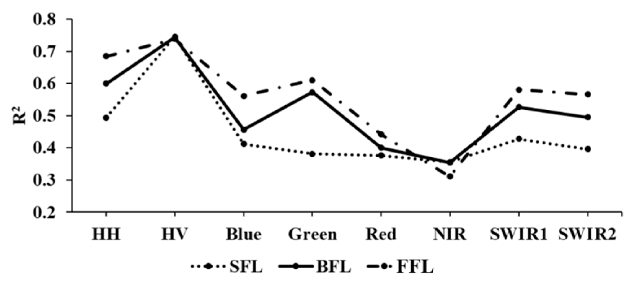
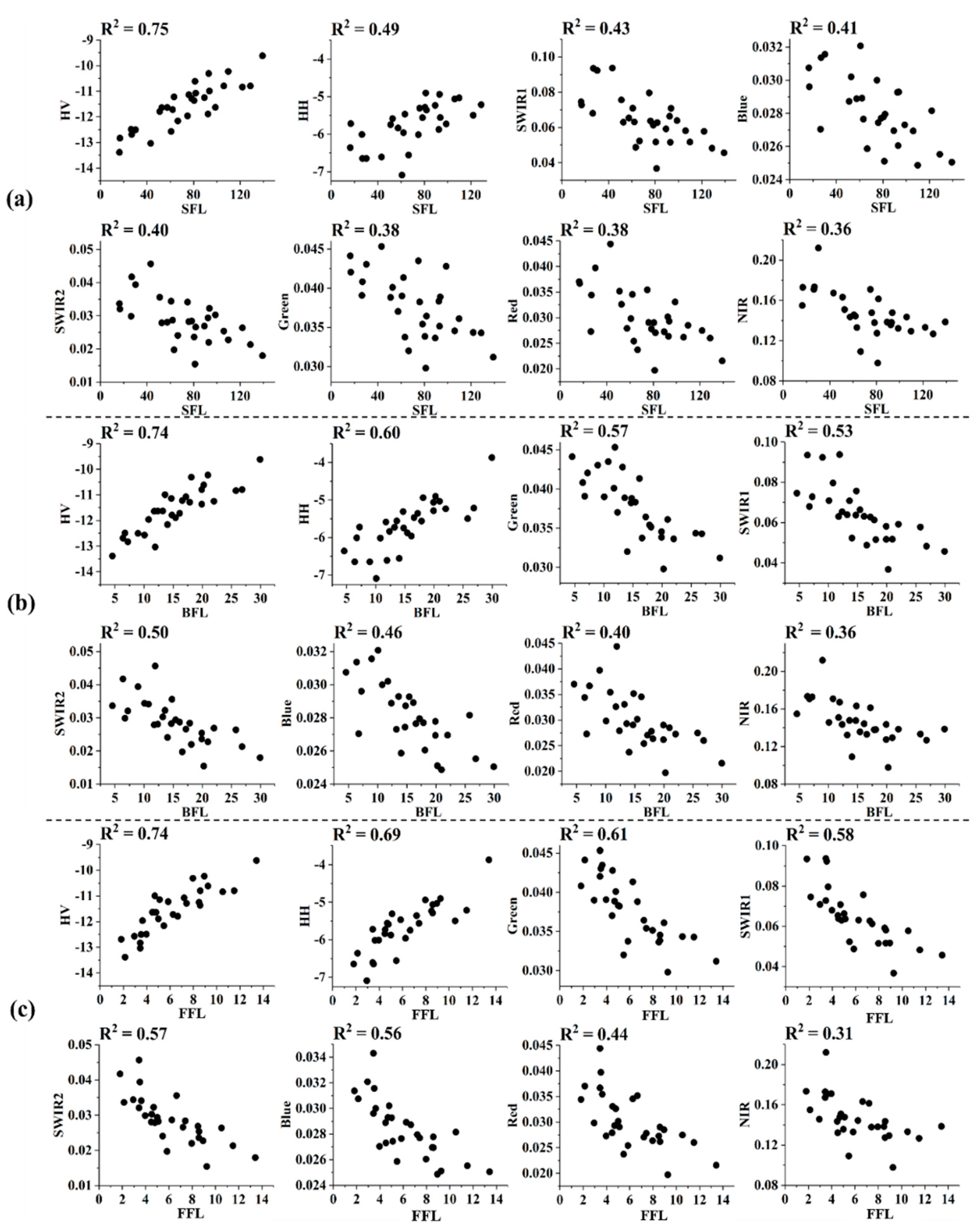
3.1. Correlation Analysis between Single Parameters and Fuel Loads

Correlation analysis was executed between the satellite data and FLs in this section, as shown in Figure 2.

For SFL, HV polarization of the L-band has the highest correlation, followed by HH polarization. Compared with SAR data, optical data generally has a lower correlation, with an average R² of about 0.4. SWIR1 has the highest correlation among the optical bands.

For BFL, the correlation trend of each parameter is similar to SFL, HV polarization of the L-band is the most sensitive variable followed by HH polarization. Among optical bands, Green and SWIR1 bands have the highest correlation, while the correlation of the optical band with BFL is higher than that of SFL.

For FFL, both HV and HH polarizations can indicate it well. All optical bands are more correlated with FFL than SFL or BFL, especially the Green band. The SWIR1 and SWIR2 bands also have a high correlation with FFL, producing an R² of about 0.6.

Overall, the HV polarization of L-band SAR data has the highest correlation with three types of forest fuel loads, and there is almost no correlation difference between different FLs. As for optical data, most bands have the highest correlation with FFL, followed by BFL, and the lowest for SFL. Specifically, the Green band has a poor correlation with SFL but a relatively high correlation with BFL and FFL. The results are reasonable since the optical signal mainly comes from the foliage in the forest canopy.

More detailed information on the relationships between satellite data and FLs is shown in Figure 3. It can be found from Figure 3a that both HV and HH polarizations increase with increasing SFL. The HV polarization has a strong positive correlation with SFL where the R² is 0.75, while the HH backscattering coefficient has a relatively weaker positive relationship with SFL. In contrast, optical data have a weak negative correlation with SFL and the correlation is not as good as SAR data. Figure 3b shows scatter plots between parameters and BFL. Similar to SFL, HV shows a strong positive relationship with BFL, while optical data shows a relatively weaker negative relationship with BFL. A similar correlation trend can also be found in Figure 3c. However, we found optical data and HH polarization have a higher correlation with FFL than that of BFL and SFL. Spectral information can express FFL as more representative than SFL and BFL. These analyses may indicate that optical data are more suitable for FFL estimation but less so for SFL or BFL.

3.2. Fuel Load Estimation from Satellite Data

Through the correlation analysis between the satellite data and FL in the previous section, it is found that the highest correlation with each kind of fuel load is HV polarization. Additionally, the relationship of optical data to FFL, BFL and SFL is weakened in turn. Figure 4 shows the results of further study on the capability of satellite data to estimate various FLs using optical bands, SAR data and both of them, respectively. The R² in Figure 4 is the optimal result of the combination situation of each number parameter in Table 2. Take the SFL estimation using both optical and SAR data as an example, the R² is 0.76 when the number of parameters is three, indicating that the best result was achieved when combining HV, NIR and SWIR2 variables.

For SFL, the estimation effect of all optical bands is not good; the average R² is 0.36, among which SWIR1, NIR and Blue bands are the variables with the highest frequency, while SAR has a good performance on SFL, and the prediction accuracy R² of a single HV polarization reaches 0.71. When combining two kinds of satellite data, as the number of parameters increases, the R² slightly increases especially when NIR and SWIR2 are added based on HV, but then it begins to decrease. Compared to the individual SAR data (HV), the combination of optical and SAR data has little effect, with the R² only increased by 0.04. This indicates that optical data cannot provide more information to characterize SFL than SAR data, and the introduction of more optical parameters will bring more errors and uncertainties, resulting in a decrease in model accuracy. Therefore, it is recommended to use only SAR data or introduce a few optical variables to carry out SFL estimation.

For the BFL, the performance of optical data is better than SFL. When selecting Green, Red and SWIR1 bands, the R² reaches 0.56, and the Green band appears in every optimal model. The performance of SAR data is slightly inferior to that of SFL, but it can also characterize BFL well, especially HV polarization (R² = 0.70). As for the combination of them, the trend of the R² is similar to that of SFL; the accuracy will not always increase with the increase in variables but tends to slightly decrease. When a model is composed of six variables or more, the performance of predicting BFL begins to decrease since more variables may introduce uncertainty to the estimation. Compared to individual SAR data (HV), the combination of optical and SAR data (i.e., HV, Green and red) has a positive effect, with the R² increased by about 0.1. This indicates that optical data also contributes to the estimation of BFL. Therefore, the BFL estimation can mainly focus on SAR data and the combination appropriate spectral bands.

For FFL, the optical spectral bands perform best with an R² of 0.66 when Blue, Green and Red bands are combined. The Green band is the best indicator of FFL among the six bands, followed by Blue. Additionally, SAR can predict FFL well individually. Besides, the addition of optical data to SAR has significantly improved the model performance (R² = 0.82) and outperformed any single data. The biggest contribution to the FFL estimate comes from HV, Green, HH and Red. However, after the number of variables is greater than four, the prediction accuracy tends to be stable and no longer increases. This is because that combination already contains the main information required by the FFL which not only has the forest structure information reflected by HV and HH, but also the spectral reflection information reflected by the optical band. Therefore, the FFL estimation should combine optical (especially the visible bands) and SAR (especially the HV polarization) data.

Overall, SAR data performed better for three types of FLs than optical, which is consistent with the correlation analysis in the previous section, while the combination of the two kinds of satellite data is better than either data alone. It is worth noting that the prediction accuracy of SFL had a clear downward trend with the increase in variables, while BFL and FFL had no such phenomenon. Besides, it was found that the most sensitive variables for the three types of FLs are different, indicating it is necessary to estimate them separately according to fuel load features (e.g., vertical structure in the forest) and different imaging mechanisms.

The relationships between variables explored in this study are shown in

Table 3. Relationship between parameters, the R² higher than 0.75 were displayed in bold font.

	Blue	Green	Red	NIR	SWIR1	SWIR2	HH	HV
Blue	--
Green	0.62	--
Red	0.69	0.85	--
NIR	0.44	0.53	0.53	--
SWIR1	0.76	0.72	0.76	0.72	--
SWIR2	0.78	0.72	0.78	0.58	0.96	--
HH	0.59	0.42	0.40	0.20	0.54	0.59	--
HV	0.61	0.55	0.54	0.30	0.58	0.61	0.78	--

and R² higher than 0.75 displayed in bold font. It is found that the closer the wavelength is, the higher the correlation between variables, such as SWIR1 and SWIR2, Green and Red. In contrast, the correlation between optical band data and SAR polarization data is relatively low. Specifically, the correlation between HV and the data of various optical bands is relatively low, especially with NIR. This may explain the phenomenon that the combination of HV and optical band can improve the FL prediction since they can carry more information on the FL than any single data. However, the correlation between different variables is generally high, probably because the study sites in this experiment are stand scale which reduces the regional heterogeneity of the remote sensing data. In the final prediction FL model selection, we select as few variables as possible (less than three) while considering the model performance to make the model more concise and avoid the introduction of redundant errors.

Based on the analyses above, we comprehensively considered the model performance and correlation between variables. A total of nine models including Opt, SAR and SAR + Opt prediction models for SFL, BFL and FFL are selected. Each selected optimal model corresponds to no more than three parameters (i.e., FLs estimated by optical data alone choose the best model composed of three parameters; FLs estimated by SAR data alone choose the model composed of two parameters; FLs estimated by both optic and SAR data choose the best model composed of three parameters), and the corresponding parameters are all contributing the most. The detailed performance of these models is shown in

Table 4. Fuel load estimation models. RMSE: root mean square error; rRMSE: relative RMSE.

Fuel Load	Variable Source	Model	R2	RMSE (Tons/ha)	rRMSE
SFL	Optical	$-4803.31\times \mathrm{Blue}-289.62\times \mathrm{NIR}-465.76\times \mathrm{SWIR}1+281.59$	0.37	25.50	0.35
	SAR	$-14.02\times \mathrm{HH}+40.40\times \mathrm{HV}+460.86$	0.72	17.00	0.23
	SAR+Optical	$-568.46\times \mathrm{NIR}+2099.73\times \mathrm{SWIR}2+36.00\times \mathrm{HV}+512.61$	0.76	15.76	0.22
BFL	Optical	$-1443.96\times \mathrm{Green}+836.04\times \mathrm{Red}-246.64\times \mathrm{SWIR}1+60.54$	0.56	4.10	0.26
	SAR	$5.97\times \mathrm{HV}+84.48$	0.70	3.33	0.21
	SAR+Optical	$-1288.38\times \mathrm{Green}+797.83\times \mathrm{Red}-5.15\times \mathrm{HV}+99.56$	0.80	2.74	0.17
FFL	Optical	$-726.45\times \mathrm{Blue}-716.35\times \mathrm{Green}+400.67\times \mathrm{Red}+41.73$	0.66	1.67	0.27
	SAR	$1.33\times \mathrm{HH}+1.87\times \mathrm{HV}+35.42$	0.72	1.49	0.24
	SAR+Optical	$-589.02\times \mathrm{Green}+326.09\times \mathrm{Red}+2.2\times \mathrm{HV}+44.06$	0.79	1.30	0.21

and Figure 5.

Single optical data has the best prediction effect on FFL (R² = 0.66) and the worst performance on SFL prediction (R² = 0.37), while single SAR data performs similarly to SFL, BFL and FFL predictions (R² = 0.72, 0.70, 0.72). Compared with the estimation with single SAR data, the addition of optical data has significantly improved the estimation accuracy for BFL and FFL (R² increased by 0.1 and 0.07), but slightly for SFL (R² increased by 0.04). Moreover, integrated L-band SAR and optical data can estimate three types of FL better than any single data (R² = 0.76, 0.80, 0.79), indicating that the combination of optical spectral information (especially the Green, Red and SWIR2 bands), and SAR data polarization information (especially HV polarization), can describe the forest fuel load well.

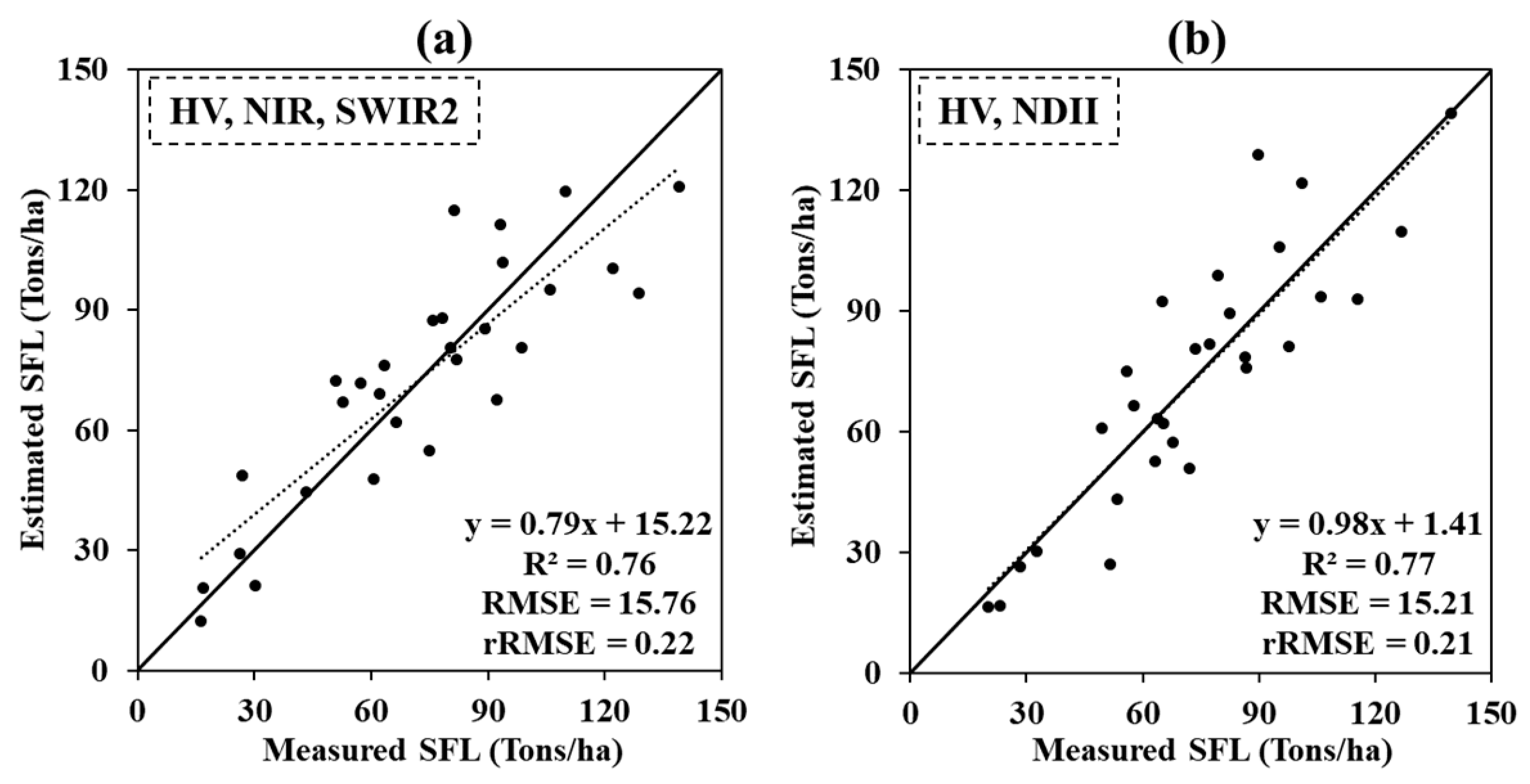
3.3. Comparison between VI and Spetral Bands

Based on the best model of SFL estimation in Section 3.2, we conducted a case experiment for SFL estimation to further compare the performance of the VI and spectral bands. This experiment also used PLSR and was validated by LOOCV. The bands used for this experiment were NIR and SWIR2 (the most sensitive spectral bands to SFL), and the VI used was the NDII, which is composed of NIR and SWIR2 bands.

$$NDII=\frac{\left(NIR-SWIR2\right)}{\left(NIR+SWIR2\right)},$$

(10)

Figure 6 shows the SFL estimation results using the combination of HV and spectral bands, and the combination of HV and the VI, respectively. It can be found that these two experiments achieved similar accuracy (R² = 0.76, 0.77), which indicates that the VI does not bring significant accuracy improvement.

4. Discussion

The definition of canopy fuel load is not uniform in different studies. In previous studies, the researchers considered the canopy fuel load as the foliage fraction alone [60], or foliage and very fine branches with a diameter less than 0.63 cm [16,61], or foliage and all branches [19,20,21], etc. Therefore, starting from the physical essence of fuel load (dry weight of fuel per unit area) and previous studies [16,19,20,21], we consider the canopy fuel load as the sum of foliage and branch dry weight, and further define the above-ground forest fuel load as a sum of SFL, BFL and FFL. Although small and flammable fuels are consumed early in the fire, the burning intensity of the fire is mainly determined by large fuels such as thick branches or even trunks which provide more flammable substances to the fire and cause greater harm.

The results of this study show that the HV polarization of L-band SAR data and the Green, Red and SWIR2 bands of optical data are suitable for FL estimation. However, the best variables varied among the three types of FL estimation, which is attributed to their spatial structure position in the forest stand and the detection characteristics of satellite data. This indicates that it is necessary to select appropriate parameters to estimate SFL, BFL and FFL separately.

Specifically, for the estimation of SFL, HV has the main contribution, and the addition of optical data does not notably improve the estimation accuracy. This is because the long-wavelength SAR data can penetrate the forest canopy and detect the stem, while the penetrating ability of optical data only captures the information on the top of the canopy [62,63] and contain less information about SFL.

The selected best model component variables for predicting the spatial distribution of SFL are HV, SWIR2 and NIR which is consistent with the result [64] that NIR and SWIR2 bands indicate biomass well (Figure 4). For the estimation of BFL, the addition of spectral information (Green and Red bands) has significantly improved the results (R² was increased by about 0.1). The optical data is more suitable to estimate BFL than SFL due to their different spatial position distributed along with tree vertical structure. Branches can influence standing woody material geometrical features which change optical spectral information [38]. However, not all spectral bands help to improve BFL estimation. As the number of optical variables increases to a certain extent, the prediction performance of the model slightly decreases. It seems that too many variables may introduce more estimation uncertainty. For the estimation of FFL, both HV and HH contribute greatly, and adding optical data (Green and Red bands) significantly improves the results (R² was increased by about 0.12). Since foliage distributes at the top of the canopy, the canopy biophysical features such as pigment content have a significant influence on optical reflectance [65].

The field sample of this study is the 29 stand scale data. These data are representative although the numbers are relatively small. The datasets have been used and validated for biomass estimation in different studies [66,67,68]. Figure 7. shows the FL value distribution of 29 stands. It can be found that these stands cover a wide range of FL values.

This study focuses on exploring the utility of different satellite data as well as their combination for fuel load estimation. For optical data, we only analyzed the spectral bands but not vegetation indices (VIs). On one hand, spectral bands contain the original information, while VIs are derived from them by the different combinations of bands and formats. The results on spectral band selection for different FLs could provide a reference for the band selection of VIs construction. On the other hand, although VIs could help to alleviate some of the atmosphere and under layer influence which may help to further improve FL estimation, we think that the linear combination of optical bands can already utilize most of the usable information for FL estimation, and the additional use of VIs may not bring significant accuracy improvement. The results in Section 3.3 demonstrated this hypothesis that the band selection is effective for VIs selection and the VI does not bring significant accuracy improvement compared with spectral bands.

In the future, the performances of VIs, derivatives of SAR data, and the multi-temporal data, especially data covering the vegetation growth phenology cycle, are conducive to the estimation of FL [69] and will be further explored. Moreover, the long time series feature of these derivatives on fuel load estimation will also be explored in the future as there have been studies using time series information of optical data to detect forest disturbances [70,71] and have achieved great success. In this study, the applicability of SAR data is only evaluated at the L-band. The spaceborne polarimetric radar measurements at other wavelengths such as the P-band and C-band can be used as a potential tool for FL estimation [72,73].

5. Conclusions

This study integrated ALOS PALSAR L-band SAR and Landsat ETM+ optical data to estimate FLs and explored their performance on SFL, BFL, and FFL estimation at the stand scale in mixed coniferous forest. Based on the PLSR and LOOCV methods, we found that the variables sensitive to the three types of forest FLs are different. The optical data is more suitable for BFL and FFL estimation than that of SFL. The SAR data performed best for SFL estimation, followed by BFL and FFL. Specifically, the Green and Red bands contribute significantly to the BFL and FFL, and the SWIR2 band contributes the most to the SFL in this landscape. HV polarization is the variable that contributes the most to all three types of FL. The combination of appropriate optical and SAR data can further improve estimations. However, the accuracy did not always increase by using more variables, and it generally decreased when all variables were used. Therefore, predictor selection in FL estimation is important and necessary. The analyses in this study can provide valuable information for the predictor selection of FL estimation. The production of high accuracy FL spatiotemporal distribution information is the crucial factor for fire risk assessment and guide the fuel management for fire suppression and response, such as prescribed burning, and increasing the distance between fuels.

References

1. Bowman, D.M.B.; Balch, J.K.; Artaxo, P.; Bond, W.J.; Carlson, J.M.; Cochrane, M.A.; D’Antonio, C.M.; Defries, R.S.; Doyle, J.C.; Harrison, S.P.; et al. Fire in the earth system. Science 2009, 324, 481–484. [Google Scholar] [CrossRef]
2. Pausas, J.G.; Keeley, J.E. Wildfires as an ecosystem service. Front. Ecol. Environ. 2019, 17, 289–295. [Google Scholar] [CrossRef] [Green Version]
3. Yebra, M.; Chuvieco, E.; Riaño, D. Estimation of live fuel moisture content from MODIS images for fire risk assessment. Agric. For. Meteorol. 2008, 148, 523–536. [Google Scholar] [CrossRef]
4. Bowman, D.M.J.S.; Moreira-Muñoz, A.; Kolden, C.A.; Chávez, R.O.; Muñoz, A.A.; Salinas, F.; González-Reyes, Á.; Rocco, R.; De La Barrera, F.; Williamson, G.J.; et al. Human–environmental drivers and impacts of the globally extreme 2017 Chilean fires. Ambio 2019, 48, 350–362. [Google Scholar] [CrossRef]
5. Jolly, W.M.; Cochrane, M.A.; Freeborn, P.H.; Holden, Z.A.; Brown, T.J. Climate-induced variations in global wildfire danger from 1979 to 2013. Nature Commun. 2015, 6, 1–11. [Google Scholar] [CrossRef]
6. David, B. Wildfire science is at a loss for comprehensive data. Nature 2018, 560, 7–8. [Google Scholar]
7. Keeley, J.E.; Van Mantgem, P.; Falk, D.A. Fire, climate and changing forests. Nat. Plants 2019, 5, 774–775. [Google Scholar] [CrossRef]
8. Byram, G. Combustion of forest fuels. In Forest Fire Forest Fire: Control Use; McGraw-Hill: New York, NY, USA, 1959; pp. 61–89. [Google Scholar]
9. Thomas, P. The size of flames from natural fires. Symp. (Int.) Combust. 1963, 9, 844–859. [Google Scholar] [CrossRef]
10. Stocks, B.J.; Wotton, B.M.; Stefner, C.N.; Flannigan, M.D.; Taylor, S.W.; Lavoie, N.; Mason, J.A.; Hartley, G.R.; Maffey, M.E.; Dalrymple, G.N.; et al. Crown fire behaviour in a northern jack pine–black spruce forest. Can. J. Forest Res. 2004, 34, 1548–1560. [Google Scholar] [CrossRef] [Green Version]
11. Pollet, J.; Omi, P.N. Effect of thinning and prescribed burning on crown fire severity in ponderosa pine forests. Int. J. Wildland Fire 2002, 11, 1–10. [Google Scholar] [CrossRef]
12. Andersen, H.-E.; McGaughey, R.J.; Reutebuch, S.E. Estimating forest canopy fuel parameters using LIDAR data. Remote Sens. Environ. 2005, 94, 441–449. [Google Scholar] [CrossRef]
13. Brandis, K.; Jacobson, C. Estimation of vegetative fuel loads using Landsat TM imagery in New South Wales, Australia. Int. J. Wildland Fire 2003, 12, 185–194. [Google Scholar] [CrossRef]
14. Mitsopoulos, I.D.; Dimitrakopoulos, A.P. Allometric equations for crown fuel biomass of Aleppo pine (Pinus halepensis Mill.) in Greece. Int. J. Wildland Fire 2007, 16, 642–647. [Google Scholar] [CrossRef]
15. Keane, R.E.; Burgan, R.; van Wagtendonk, J. Mapping wildland fuels for fire management across multiple scales: Integrating remote sensing, GIS, and biophysical modeling. Int. J. Wildland Fire 2001, 10, 301–309. [Google Scholar] [CrossRef]
16. Mallinis, G.; Mitsopoulos, Ι.; Stournara, P.; Patias, P.; Dimitrakopoulos, A.; Mitsopoulos, I. Canopy Fuel Load Mapping of Mediterranean Pine Sites Based on Individual Tree-Crown Delineation. Remote Sens. 2013, 5, 6461–6480. [Google Scholar] [CrossRef] [Green Version]
17. Lucas, R.; Van De Kerchove, R.; Otero, V.; Lagomasino, D.; Fatoyinbo, L.; Omar, H.; Satyanarayana, B.; Dahdouh-Guebas, F. Structural characterisation of mangrove forests achieved through combining multiple sources of remote sensing data. Remote Sens. Environ. 2020, 237, 111543. [Google Scholar] [CrossRef]
18. Kganyago, M.; Shikwambana, L. Assessment of the Characteristics of Recent Major Wildfires in the USA, Australia and Brazil in 2018–2019 Using Multi-Source Satellite Products. Remote Sens. 2020, 12, 1803. [Google Scholar] [CrossRef]
19. Baysal, I.; Yurtgan, M.; Küçük, Ö.; Öztürk, N. Estimation of Crown Fuel Load of Suppressed Trees in Non-treated Young Calabrian Pine (Pinus brutia Ten.) Plantation Areas. Kast. Üniversitesi Orman Fakültesi Derg. 2019, 19, 351–360. [Google Scholar] [CrossRef] [Green Version]
20. Kucuk, O.; Bilgili, E.; Sağlam, B. Estimating crown fuel loading for calabrian pine and Anatolian black pine. Int. J. Wildland Fire 2008, 17, 147–154. [Google Scholar] [CrossRef]
21. Kucuk, O.; Saglam, B.; Bilgili, E. Canopy Fuel Characteristics and Fuel Load in Young Black Pine Trees. Biotechnol. Biotechnol. Equip. 2007, 21, 235–240. [Google Scholar] [CrossRef] [Green Version]
22. Arellano-Pérez, S.; Castedo-Dorado, F.; López-Sánchez, C.A.; González-Ferreiro, E.; Yang, Z.; Díaz-Varela, R.A.; Álvarez-González, J.G.; Vega, J.A.; Ruiz-González, A.D. Potential of Sentinel-2A Data to Model Surface and Canopy Fuel Characteristics in Relation to Crown Fire Hazard. Remote Sens. 2018, 10, 1645. [Google Scholar] [CrossRef] [Green Version]
23. Scott, J.H.; Reinhardt, E.D.; Station, R.M.R. Assessing Crown Fire Potential by Linking Models of Surface and Crown Fire Behavior; U.S. Department of Agriculture, Forest Service, Rocky Mountain Research Station: Fort Collins, CO, USA, 2001. [CrossRef] [Green Version]
24. Güngöroglu, C.; Serttaş, A.; Sari, A.; Güney, Ç.O. Predicting crown fuel biomass of Turkish red pine (Pinus brutia Ten.) for the Mediterranean regions of Turkey. Šumarski List 2018, 142, 610. [Google Scholar] [CrossRef]
25. Reich, R.M.; Lundquist, J.E.; Bravo, V.A. Spatial models for estimating fuel loads in the Black Hills, South Dakota, USA. Int. J. Wildland Fire 2004, 13, 119–129. [Google Scholar] [CrossRef]
26. Stow, D.; Hope, A.; McKinsey, D.; Pray, H. Deriving dynamic information on fire fuel distributions in southern Californian chaparral from remotely sensed data. Landsc. Urban. Plan. 1993, 24, 113–127. [Google Scholar] [CrossRef]
27. Chen, Y.; Zhu, X.; Yebra, M.; Harris, S.; Tapper, N. Development of a predictive model for estimating forest surface fuel load in Australian eucalypt forests with LiDAR data. Environ. Model. Softw. 2017, 97, 61–71. [Google Scholar] [CrossRef]
28. González-Ferreiro, E.; Arellano-Pérez, S.; Castedo-Dorado, F.; Hevia, A.; Vega, J.A.; Vega-Nieva, D.J.; Álvarez-González, J.G.; Ruiz-González, A.D. Modelling the vertical distribution of canopy fuel load using national forest inventory and low-density airbone laser scanning data. PLoS ONE 2017, 12, e0176114. [Google Scholar] [CrossRef]
29. Michel, U.; Schulz, K.; Ehlers, M.; Nikolakopoulos, K.G.; Civco, D.; Chen, Y.; Zhu, X.; Yebra, M.; Harris, S.; Tapper, N. Estimation of forest surface fuel load using airborne lidar data. In Proceedings of the Earth Resources and Environmental Remote Sensing/GIS Applications VII, Edinburgh, UK, 27–29 September 2016. [Google Scholar]
30. Skowronski, N.; Clark, K.; Nelson, R.; Hom, J.; Patterson, M. Remotely sensed measurements of forest structure and fuel loads in the Pinelands of New Jersey. Remote Sens. Environ. 2007, 108, 123–129. [Google Scholar] [CrossRef]
31. Jin, S.; Chen, S.-C. Application of QuickBird imagery in fuel load estimation in the Daxinganling region, China. Int. J. Wildland Fire 2012, 21, 583–590. [Google Scholar] [CrossRef]
32. Lai, X.Q.Y.L.B.H.G.C.G. Application of Landsat ETM+ and OLI Data for Foliage Fuel Load Monitoring Using Radiative Transfer Model and Machine Learning Method. IEEE J. Sel. Top. Appl. Earth Obs. Remote Sens. 2021, 99, 1. [Google Scholar]
33. Saatchi, S.; Halligan, K.; Despain, D.G.; Crabtree, R.L. Estimation of Forest Fuel Load From Radar Remote Sensing. IEEE Trans. Geosci. Remote Sens. 2007, 45, 1726–1740. [Google Scholar] [CrossRef]
34. Cho, M.A.; Mathieu, R.; Asner, G.P.; Naidoo, L.; Van Aardt, J.; Ramoelo, A.; Debba, P.; Wessels, K.; Main, R.; Smit, I.P.; et al. Mapping tree species composition in South African savannas using an integrated airborne spectral and LiDAR system. Remote Sens. Environ. 2012, 125, 214–226. [Google Scholar] [CrossRef]
35. Lefsky, M.A.; Hudak, A.T.; Cohen, W.B.; Acker, S. Geographic variability in lidar predictions of forest stand structure in the Pacific Northwest. Remote Sens. Environ. 2005, 95, 532–548. [Google Scholar] [CrossRef] [Green Version]
36. Cartus, O.; Santoro, M.; Kellndorfer, J. Mapping forest aboveground biomass in the Northeastern United States with ALOS PALSAR dual-polarization L-band. Remote Sens. Environ. 2012, 124, 466–478. [Google Scholar] [CrossRef]
37. Evans, J.P.; Guojie, W. Recent reversal in global terrestrial biomass loss. Nat. Clim. Chang. 2015, 5, 470–474. [Google Scholar]
38. Massetti, A.; Rüdiger, C.; Yebra, M.; Hilton, J. The Vegetation Structure Perpendicular Index (VSPI): A forest condition index for wildfire predictions. Remote Sens. Environ. 2019, 224, 167–181. [Google Scholar] [CrossRef]
39. Bai, X.; He, B.; Li, X.; Zeng, J.; Wang, X.; Wang, Z.; Zeng, Y.; Su, Z. First Assessment of Sentinel-1A Data for Surface Soil Moisture Estimations Using a Coupled Water Cloud Model and Advanced Integral Equation Model over the Tibetan Plateau. Remote Sens. 2017, 9, 714. [Google Scholar] [CrossRef] [Green Version]
40. Wang, L.; Quan, X.; He, B.; Yebra, M.; Xing, M.; Liu, X. Assessment of the Dual Polarimetric Sentinel-1A Data for Forest Fuel Moisture Content Estimation. Remote Sens. 2019, 11, 1568. [Google Scholar] [CrossRef] [Green Version]
41. Castillo, J.A.A.; Apan, A.A.; Maraseni, T.N.; Salmo, S.G. Estimation and mapping of above-ground biomass of mangrove forests and their replacement land uses in the Philippines using Sentinel imagery. ISPRS J. Photogramm. Remote Sens. 2017, 134, 70–85. [Google Scholar] [CrossRef]
42. Debastiani, A.B.; Sanquetta, C.R.; Corte, A.P.D.; Pinto, N.S.; Rex, F.E. Evaluating SAR-optical sensor fusion for aboveground biomass estimation in a Brazilian tropical forest. Ann. For. Res. 2019, 62, 109–122. [Google Scholar] [CrossRef]
43. Li, X.; Li, L.; Liu, X. Collaborative inversion heavy metal stress in rice by using two-dimensional spectral feature space based on HJ-1 A HSI and radarsat-2 SAR remote sensing data. Int. J. Appl. Earth Obs. Geoinf. 2019, 78, 39–52. [Google Scholar] [CrossRef]
44. Nuthammachot, N.; Askar, A.; Stratoulias, D.; Wicaksono, P. Combined use of Sentinel-1 and Sentinel-2 data for improving above-ground biomass estimation. Geocarto Int. 2020, 10, 1–11. [Google Scholar] [CrossRef]
45. Laudon, H.; Sjöblom, V.; Buffam, I.; Seibert, J.; Mörth, M. The role of catchment scale and landscape characteristics for runoff generation of boreal streams. J. Hydrol. 2007, 344, 198–209. [Google Scholar] [CrossRef]
46. Petersson, H. Biomassafunktioner for trädfraktioner av tall, gran och björk i sverige. SLU Inst. Skoglig Resur. Och Geomatik Arbetsrapport 1999, 59. [Google Scholar]
47. Hajnsek, I.; Scheiber, R.; Keller, M.; Horn, R.; Lee, S.; Ulander, L.; Gustavsson, A.; Sandberg, G.; Le Toan, T.; Tebaldini, S.; et al. BIOSAR 2008: Final Report. ESA-ESTEC Noordwijk Neth. Tech. Rep. 2009, 8, 22052. [Google Scholar]
48. Thapa, R.B.; Watanabe, M.; Motohka, T.; Shimada, M. Potential of high-resolution ALOS–PALSAR mosaic texture for aboveground forest carbon tracking in tropical region. Remote Sens. Environ. 2015, 160, 122–133. [Google Scholar] [CrossRef]
49. Shimada, M.; Ohtaki, T. Generating Large-Scale High-Quality SAR Mosaic Datasets: Application to PALSAR Data for Global Monitoring. IEEE J. Sel. Top. Appl. Earth Obs. Remote Sens. 2010, 3, 637–656. [Google Scholar] [CrossRef]
50. Gorelick, N.; Hancher, M.; Dixon, M.; Ilyushchenko, S.; Thau, D.; Moore, R. Google Earth Engine: Planetary-scale geospatial analysis for everyone. Remote Sens. Environ. 2017, 202, 18–27. [Google Scholar] [CrossRef]
51. Shimada, M.; Itoh, T.; Motooka, T.; Watanabe, M.; Shiraishi, T.; Thapa, R.; Lucas, R. New global forest/non-forest maps from ALOS PALSAR data (2007–2010). Remote Sens. Environ. 2014, 155, 13–31. [Google Scholar] [CrossRef]
52. Scaramuzza, P.; Barsi, J. Landsat 7 scan line corrector-off gap-filled product developme. Proc. Pecora 2005, 16, 23–27. [Google Scholar]
53. Hardisky, M.A.; Klemas, V.; Smart, R.M. The influence of soil salinity, growth form, and leaf moisture on the spectral radiance of Spartina Alterniflora canopies. Photogramm. Eng. Remote Sens. 1983, 49, 77–84. [Google Scholar]
54. Wold, S.; Sjöström, M.; Eriksson, L. PLS-regression: A basic tool of chemometrics. Chemom. Intell. Lab. Syst. 2001, 58, 109–130. [Google Scholar] [CrossRef]
55. Adjorlolo, C.; Mutanga, O.; Cho, M.A. Predicting C3 and C4 grass nutrient variability using in situ canopy reflectance and partial least squares regression. Int. J. Remote Sens. 2015, 36, 1743–1761. [Google Scholar] [CrossRef]
56. Rapaport, T.; Hochberg, U.; Shoshany, M.; Karnieli, A.; Rachmilevitch, S. Combining leaf physiology, hyperspectral imaging and partial least squares-regression (PLS-R) for grapevine water status assessment. ISPRS J. Photogramm. Remote Sens. 2015, 109, 88–97. [Google Scholar] [CrossRef]
57. Kiala, Z.; Odindi, J.; Mutanga, O.; Peerbhay, K. Comparison of partial least squares and support vector regressions for predicting leaf area index on a tropical grassland using hyperspectral data. J. Appl. Remote Sens. 2016, 10, 036015. [Google Scholar] [CrossRef]
58. Ryan, K.; Ali, K. Application of a partial least-squares regression model to retrieve chlorophyll-a concentrations in coastal waters using hyper-spectral data. Ocean. Sci. J. 2016, 51, 209–221. [Google Scholar] [CrossRef]
59. Guo, Y.-J.; Han, J.-J.; Zhao, X.; Dai, X.-Y.; Zhang, H. Understanding the Role of Optimized Land Use/Land Cover Components in Mitigating Summertime Intra-Surface Urban Heat Island Effect: A Study on Downtown Shanghai, China. Energies 2020, 13, 1678. [Google Scholar] [CrossRef] [Green Version]
60. Fernandes, P.; Loureiro, C.; Botelho, H.; Ferreira, A.; Fernandes, M. Avaliação Indirecta da Carga de Combustível em Pinhal Bravo. Silva Lusit. 2002, 10, 73–90. [Google Scholar]
61. Jiménez, E.; Vega, J.A.; Fernández-Alonso, J.M.; Vega-Nieva, D.; Álvarez-González, J.G.; Ruiz-González, A.D. Allometric equations for estimating canopy fuel load and distribution of pole-size maritime pine trees in five Iberian provenances. Can. J. For. Res. 2013, 43, 149–158. [Google Scholar] [CrossRef]
62. Amini, J.; Sumantyo, J.T.S. Employing a Method on SAR and Optical Images for Forest Biomass Estimation. IEEE Trans. Geosci. Remote Sens. 2009, 47, 4020–4026. [Google Scholar] [CrossRef]
63. Svoray, T.; Shoshany, M. Herbaceous biomass retrieval in habitats of complex composition: A model merging sar images with unmixed landsat tm data. IEEE Trans. Geosci. Remote Sens. 2003, 41, 1592–1601. [Google Scholar] [CrossRef]
64. Reese, H.; Nilsson, M.; Olsson, H. Comparison of Resourcesat-1 AWiFS and SPOT-5 data over managed boreal forest stands. Int. J. Remote Sens. 2009, 30, 4957–4978. [Google Scholar] [CrossRef] [Green Version]
65. Féret, J.-B.; Le Maire, G.; Jay, S.; Berveiller, D.; Bendoula, R.; Hmimina, G.; Cheraiet, A.; Oliveira, J.; Ponzoni, F.; Solanki, T.; et al. Estimating leaf mass per area and equivalent water thickness based on leaf optical properties: Potential and limitations of physical modeling and machine learning. Remote Sens. Environ. 2019, 231, 110959. [Google Scholar] [CrossRef]
66. Blomberg, E.; Ferro-Famil, L.; Soja, M.J.; Ulander, L.M.H.; Tebaldini, S. Forest Biomass Retrieval From L-Band SAR Using Tomographic Ground Backscatter Removal. IEEE Geosci. Remote Sens. Lett. 2018, 15, 1030–1034. [Google Scholar] [CrossRef]
67. Askne, J.I.; Soja, M.J.; Ulander, L.M. Biomass estimation in a boreal forest from TanDEM-X data, lidar DTM, and the interferometric water cloud model. Remote Sens. Environ. 2017, 196, 265–278. [Google Scholar] [CrossRef]
68. Zhang, H.; Wang, C.; Zhu, J.; Fu, H.; Xie, Q.; Shen, P. Forest Above-Ground Biomass Estimation Using Single-Baseline Polarization Coherence Tomography with P-Band PolInSAR Data. Forests 2018, 9, 163. [Google Scholar] [CrossRef] [Green Version]
69. Huang, X.; Ziniti, B.; Torbick, N.; Ducey, M.J. Assessment of Forest above Ground Biomass Estimation Using Multi-Temporal C-band Sentinel-1 and Polarimetric L-band PALSAR-2 Data. Remote Sens. 2018, 10, 1424. [Google Scholar] [CrossRef] [Green Version]
70. Zhu, Z.; Woodcock, C.E.; Olofsson, P. Continuous monitoring of forest disturbance using all available Landsat imagery. Remote Sens. Environ. 2012, 122, 75–91. [Google Scholar] [CrossRef]
71. Ye, S.; Rogan, J.; Zhu, Z.; Eastman, J.R. A near-real-time approach for monitoring forest disturbance using Landsat time series: Stochastic continuous change detection. Remote Sens. Environ. 2021, 252, 112167. [Google Scholar] [CrossRef]
72. Liao, Z.; He, B.; Quan, X.; Van Dijk, A.I.; Qiu, S.; Yin, C. Biomass estimation in dense tropical forest using multiple information from single-baseline P-band PolInSAR data. Remote Sens. Environ. 2019, 221, 489–507. [Google Scholar] [CrossRef]
73. Chen, L.; Wang, Y.; Ren, C.; Zhang, B.; Wang, Z. Optimal Combination of Predictors and Algorithms for Forest Above-Ground Biomass Mapping from Sentinel and SRTM Data. Remote Sens. 2019, 11, 414. [Google Scholar] [CrossRef] [Green Version]
Figure 1. Location of the study area. The background map is the 2008 PALSAR mosaic yearly product (red: HH, green: HH+HV, blue: HV,) and red border polygons are 29 stands.
Remotesensing 13 01189 g001
Figure 2. Relationships between satellite data and stem fuel load (SFL), branch fuel load (BFL) and foliage fuel load (FFL).
Remotesensing 13 01189 g002
Figure 3. Scatterplots between satellite data and fuel loads. From top to bottom are SFL (a), BFL (b) and FFL (c), respectively. These figures were sorted by relevance from left to right.
Remotesensing 13 01189 g003
Figure 4. Parameter combination fitting results shows the best fitting results of multi-parameter models for above-ground forest fuel loads and the specific parameter combination information using optical data, SAR data, or both of them, respectively. The black solid triangles representing the R2 of the optimal model combined with the number of parameters (1 to 8), and the black solid circles representing the parameters corresponding to the right vertical axis are included in the optimal model. Each parameter on the right vertical axis corresponds to a dotted line, reflecting the frequency of the corresponding parameter in the optimal model.
Remotesensing 13 01189 g004
Figure 5. Scatterplot of estimated fuel load vs. measured fuel load. From top to bottom are SFL, BFL, FFL, and from left to right are Opt, SAR, SAR + Opt.
Remotesensing 13 01189 g005
Figure 6. Comparison of SFL estimation using (a) HV and optical bands, and (b) HV and vegetation index (VI).
Remotesensing 13 01189 g006
Figure 7. Fuel load (FL) value distribution of 29 stands.
Remotesensing 13 01189 g007