Fast and Accurate Terrain Image Classification for ASTER Remote Sensing by Data Stream Mining and Evolutionary-EAC Instance-Learning-Based Algorithm

Abstract

Remote sensing streams continuous data feed from the satellite to ground station for data analysis. Often the data analytics involves analyzing data in real-time, such as emergency control, surveillance of military operations or scenarios that change rapidly. Traditional data mining requires all the data to be available prior to inducing a model by supervised learning, for automatic image recognition or classification. Any new update on the data prompts the model to be built again by loading in all the previous and new data. Therefore, the training time will increase indefinitely making it unsuitable for real-time application in remote sensing. As a contribution to solving this problem, a new approach of data analytics for remote sensing for data stream mining is formulated and reported in this paper. Fresh data feed collected from afar is used to approximate an image recognition model without reloading the history, which helps eliminate the latency in building the model again and again. In the past, data stream mining has a drawback in approximating a classification model with a sufficiently high level of accuracy. This is due to the one-pass incremental learning mechanism inherently exists in the design of the data stream mining algorithm. In order to solve this problem, a novel streamlined sensor data processing method is proposed called evolutionary expand-and-contract instance-based learning algorithm (EEAC-IBL). The multivariate data stream is first expanded into many subspaces, and then the subspaces, which are corresponding to the characteristics of the features are selected and condensed into a significant feature subset. The selection operates stochastically instead of deterministically by evolutionary optimization, which approximates the best subgroup. Followed by data stream mining, the model learning for image recognition is done on the fly. This stochastic approximation method is fast and accurate, offering an alternative to the traditional machine learning method for image recognition application in remote sensing. Our experimental results show computing advantages over other classical approaches, with a mean accuracy improvement at 16.62%.

1. Introduction

Remote sensing (RS) is considered as a process of acquiring information about a specific target, a region, or some event through analyzing the data collected by a probe that is free of contact with the target, region, or event for investigation purpose [1]. The latest RS satellites that are capable of providing high resolution imaging data have huge potential for scientific surveillance and investigation [2]. Land type assessment is aided by RS satellites for data collection coupled with pattern classification using digital image processing and data mining techniques.

Pattern recognition is an essential part of land use or land condition classification [3]. RS data are mapped to spectral classes, which are predefined into several land types or land condition types, that are measured by the spectral radiance levels of the pixels within an area of interest [4]. Often the predefined classes are manually defined as ground-truth, by physical examination of the conditions on the ground with reference to the RS image data. Each pixel in a RS image carries certain numerical information of spectral radiance levels. In other words, a pattern in the context of RS application is a collection of radiance measurements in the format of wavelength or frequency value at each pixel. During the RS surveillance, information is relayed from one transmitter to another where the pixel-by-pixel spectral information is used. Not only the data volume is massive, they tend to change very dynamically when the view of surveillance moves [5]. Furthermore, additional information may be added, depending on the model of RS satellite and the interpretation mechanism used [6].

For relieving this latency bottleneck in RS where a massive amount of data are to be transmitted and processed, the authors proposed to use data stream mining together with a novel preprocessing mechanism that is designed to speed up the machine learning latency. Unlike traditional data mining, data stream mining learns from the new arriving data incrementally. The model refresh time is at only a fraction of that of the classical data mining. To make the model learning even faster, RS data are preprocessed with a novel feature engineering mechanism [7] called the evolutionary expand-and-contract instance-based learning algorithm (EEAC-IBL). The multivariate data stream is first expanded into many subspaces [8], then the subspaces that are corresponding to the characteristics of the features are selected and condensed into a significant subset of bags of instances. The selection operates stochastically instead of deterministically by evolutionary optimization, which approximates the best subgroup. Followed by data stream mining, the model learning for image recognition is done on the fly [9]. This stochastic approximation method is fast and accurate, offering an alternative to the traditional machine learning method for image recognition application in remote sensing.

Instance-based learning principle on which EEAC-IBL is based, has pros and cons over the traditional machine learning approach. The preprocessing approach associated with traditional machine learning often works like greedy search. It is myopic specifically to matching the attributes or the characteristics of the training data, therefore lacking optimization over most of the testing data. The advantage of instance-based learning is its ability in subtly and fuzzily placing the relevant data in bags or subspaces, in lieu of directly labeling the data with specific labels. Some flexibility is hence made possible, especially for data whose characteristics have some grey-areas or overlaps. Thereby this approach is inherently suitable for learning from data for pattern recognition, computer vision, and image classification, which are fuzzy and noisy in nature. Satellite RS data could be applicable too, since it is about dealing with images with extra performance requirement of real-time processing and memory constraints. The drawback of instance-based learning is the potential explosion of the attribute amount—many subspaces could be generated in the process that may lead to model overfitting and runtime memory overhead. EEAC-IBL has a key mechanism in first inflating the subspaces, and then evolutionary optimization is applied for shrinking them to the fittest size. EEAC-IBL is particularly useful for pattern recognition such as satellite RS, and other image recognition domains where accuracy, speed, and memory constraints are of a concern.

1.1. Contribution

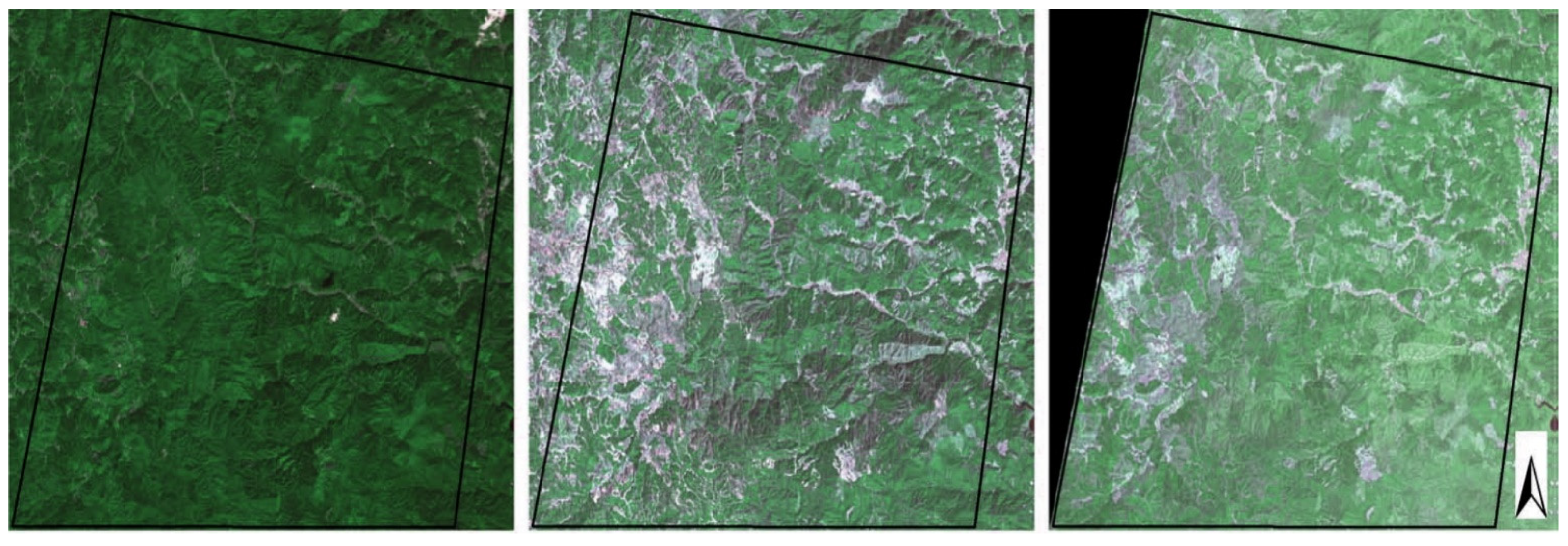
In this paper, empirical RS data were used to validate the efficacy of EEAC-IBL method in comparison to the other classical approaches. The data are mixed forest types data, collected from the advanced spaceborne thermal emission and reflection radiometer satellite [10], known as ASTER data [11]. An example is shown in Figure 1 where three images of the same forest was photographed at Ibaraki Prefecture, Japan, from ASTER satellite from space at three different times [12]. The radiance values of the spectral data mark the bare land and leaves of the forest, telling between the withering of the trees at different seasons. The difference and characteristics between the visual elements in terms of spectral values between the images such as the distribution and proximity of the leaves and lands are first remembered by a machine learning model. Then the model is tested with new images, which can tell which types the images belong to. In summary, the contributions of our study are as follows:

(1)

Our proposed method aims at streamlining the data preprocessing overhead for efficient remote sensing.

(2)

The advantage is to achieve minimum latency in real-time RS monitoring, by making the machine learning fast and accurate enough.

1.2. Motivation

Rather than focusing on individual data instance and their features values, bagging [13] allows us working on subspaces of samples, which are transformed from raw data instances to quality ingredients for model training. One obvious shortcoming of the bagging method is the inflation of data size in the magnitude of ten folds or more. This data instance space expansion to inflated subspaces must be kept under control. Hence a new mechanism called the expand-and-contract instance-based learning (EAC-IBL) algorithm is formulated to solve this problem. As the name suggested, it has dual steps, which first inflates the data instances into bags or subspaces, and then a fast feature selection is performed over the subspaces for shrinking them to a compact level, suitable for fast model learning even in the data streaming mode. The own dual-steps process is controlled by an evolutionary optimization method [14], which stochastically tries to find the most optimal configuration of subspaces and the selected subspaces in a timely manner. As such the new method is called evolutionary expand-and-contract instance-based learning (EEAC-IBL) algorithm. In this paper, EEAC-IBL is shown to be simpler than the prior-arts, yet it yields profound performance as a result in classifying RS data from a multidimensional data stream generated from ASTER. Based on multiple instance learning [15], EEAC-IBL is a simple approach in converting the attributes values pertaining to a specific class of land-type into subspaces to be added into training data. The additional subspaces information is the statistical representation of the time-series pattern taken from that attribute whose sequential values within that class label indeed form a time-series.

On the other hand, the use of data stream mining is another motivation in the face of the latency problem associated with machine learning in the traditional data mining approach. A machine learning model will gradually lose its efficacy due to long use where too much unseen data has come since the last model update. Periodically a traditional data mining model needs to refresh itself by loading the full historical dataset plus the latest data for rebuilding the whole model. This regular model rebuilt will take an increasingly long time, as the total data volume grows in time. A new generation of machine learning that has low learning latency and is suitable for real-time applications such as pattern recognition in RS is needed. Therefore, data stream mining, which induces a pattern recognition model by incremental learning over continuous data feed is explored in this study.

2. Related Works

Two main related works are introduced here—pattern recognition in RS and the EEAC-IBL algorithm. The former process is the core of machine learning in RS, where a supervised learning is trained and subsequently used for identifying the land type upon seeing new images. The latter is the main mechanism for fast-and-accurate preprocessing for boosting accuracy and reducing latency in RS.

2.1. Pattern Recognition

Traditionally, visual elements are being used as variables that characterize collectively and spatially the nature or type of a target area Information extracted from the collected RS images would be evaluated in the forms of pixel proximity with reference to the overall image and its neighbor pixels, shape, image texture, color, light, distinctive and repetitive patterns, directionality, etc. In general, they are known or referred as spectral images, which are image patterns with spatial relationship in the proximity among representative subsets of pixels, which are numeric, altogether they come in huge sizes and volumes during the remote sensing operation. The data volume of RS data is ever increasing in quantities as RS operation progresses. They accumulate into very large data, which lead to data processing problems making data mining tasks difficult especially in rebuilding the models and the latency introduced.

In pattern recognition, image classification works by building a predictive model by machine learning; once a representative model matures by seeing enough training samples, some non-linear mappings between the input variable values from the training data and the predefined land use types are formed. New data, which are called testing data, could be subjected to the predictive model, which automatically classify the testing data into one of the predefined groups of land use labels. Testing (classifying the new images into classes) is usually very fast but constructing a model by letting it see all the training images takes time. This conventional mode of machine learning has one major drawback—each time new images are to be included in the training samples, the model needs to reload all the training data (both old and new) and rebuilds itself from scratch. The latency will prolong when more and more training samples are to be embraced as RS operates. The learning time becomes longer than its previous round as time elapses.

2.2. EEAC-IBL Algorithm

The conventional supervised learning model is invented on the basis of mapping the non-linear relation between the input variables or features and the labeled output through a certain number of data instances. Since decades ago, researchers have been focusing on inventing and improving new models, which are robust and accurate, assuming that the underlying input–output relation in the training data remains rigid and strong.

Unfortunately, this is not always true that well-preserved input–output relations can be found in training data. Recent paradigms of machine learning applications involve training data that are loosely structured and highly ambiguous [16,17]. For instance, the boundaries of image data in image recognition are naturally vague. An emerging machine learning over some collection of RS data for distinguishing different landscapes from the spectral data exhibits similar challenge. The boundary, which is made up of certain data instances between various classes of data or concepts, is blurred. So, modeling such discrimination that lies over overlaps and ambiguity of data instances should be made flexible.

An alternative type of machine learning was therefore proposed, which is known as multiple instance learning [18] for handling training data with vague segregation. Instead of individual pairs of input–output data records, this new learning method works on bags or subspaces with designated labels or classes each containing certain data instances. A basic rule for bagging up the data instances is that at least one data instance of positive class (or a target label) can be found in every positive bag, possibly mixing with data instances of other classes; and no positive data instance exists in every negative bag. In other words, negative bags must contain only negative data instances or data instances, which never belong to the target class. Machine learning is then trained by loading these bags or subspaces of data instances in lieu of the raw data instances. As such, ambiguity is embraced in a way that the trained model recognizes the polarity or classes of bags at an abstract level (data group or data subspace) rather than individually at the data instance level.

This type of alternative supervised learning is receiving increasing research attention; most of the endeavors were spent on image recognition where no tightly defined of point of interest is needed but numerous possibilities exist in outlining the area of interest; and on drug discovery where there are potentially many ways of folding the chemical molecules and docking by infinity functions.

However, to the best of the authors’ knowledge, the work reported in this paper should be one of the pioneers in applying subspace machine learning on RS data for image recognition over land-types. The nature of the machine learning task over RS data feeds is full of ambiguity, for which no traditional supervised learning can achieve reasonable accuracy.

3. Problem Description

The problem to be solved for this particular case of RS data mining for recognizing land-types can be as follows. The machine learning model is generic, which could be any supervised learning model, which loads a set of training dataset for learning; once matured it will be used for testing new unseen data. The classification model is deployed here, which classifies the unseen (testing) data instances as one of the predefined classes as output.

In this case, the predefined classes are land-types, which are labeled by human experts. The inputs are RS data collected from the ASTER satellite where data streams of multiple attributes are generated from the imaging. Each data instance collected from the satellite may have one or more features or attributes that describe the frequency spectrum of the data. Summing up the features from all the frequencies, the data stream is a combination of RS data of frequency values, which reflect the visual elements of the land that is currently being scanned. Each data vector is a combination of RS data that could be used for image classification—there are a total of 27 features, out of which 9 features are spectral bands, and the other 18 features are the pseudo values. The pseudo values are the similarity measures computed from the interpolated values found by inverse distance weighting.

A training dataset is therefore an m × n matrix of the m dimension of the data matrix or m number of features. The m number of features is the sum of all the possible features taken from all the spectral bands including their pseudo representatives by inverse distance weighting. The labels in the training dataset are annotated by a human beforehand by his expert judgment. There is a total of n data tuples in a training dataset. In fact, n → ∞ potentially because the satellite may be operating without interruption, so the data stream is unbounded.

For simplicity, we let n be a whole integer, which is typically hundreds of thousands given the sampling rate is less than a second, and the data stream is being collected for a certain length of time. Corresponding to each tuple of data instance where $\left\{x_1, x_2 \dots , x_n \right\} \mathrm{where} x_i\in X \mathrm{and}$ each x_i is characterized by m features $x_i\leftarrow {\left\{f_1, f_2 \dots , f_m \right\}}_i$ there exists a multidimensional and non-linear Euclidean space S at the order d, $X=S^d$, and the classification labels are $\left\{y_1, y_2 \dots , y_n\right\}$ with respect to the possible classes of land-type where $y_i\in Y$.

For supervised learning, the model is simply a function that can be implemented by different machine learning algorithms, from the simplest naive Bayes to most sophisticated deep learning, where F(X): X → Y, which models the relations between X and Y by inducing the mapping → between the input and output.

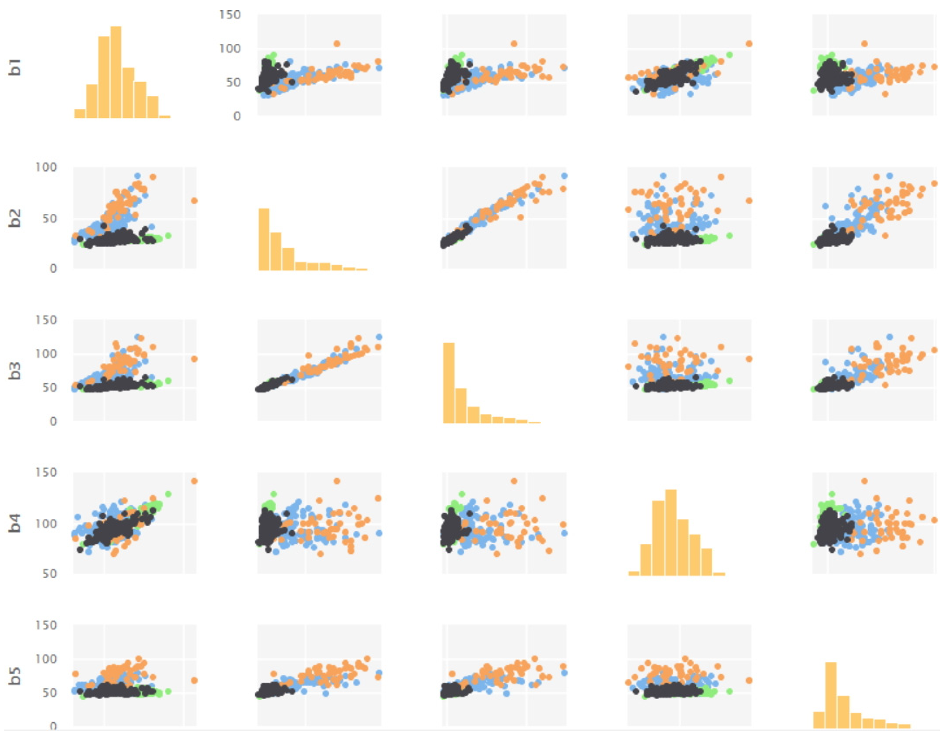
From a simple data visualization from the RS data collected from the ASTER satellite, one can see from Figure 2 that the activities labels were very much mixed and interleaved across different features values. Such non-linearity therefore contributes to a Euclidean data space. This posed a good level of challenges in machine learning for learning up a useful model.

Once the dataset is transformed into the subspace by instance-based learning or multiple instance learning, the data instances are grouped into bags; hence the training dataset is a collection of bags $\left\{b_1, b_2 \dots , b_o\right\}$ and the bag labels are $\left\{e_1, e_2 \dots , e_o\right\}$, o is the number of bags generated and often o >> the number of predefined class labels (land-types). The basic assumption of instance-based learning applies, that is, a subspace is considered positive if and only if it has one or more data instances inside the bag that is positive.

Here we define the meaning or implication of being positive is that the predicted land-type is the land-type of interest. Additionally, when there exists none of the positive instance in a bag, the bag then is considered as zero in value that implies the bag has instances of any land-type but the one that is of interest. The predicted class of bag then takes the following value in generalization:

$$e_{\alpha }=\underset{\beta }{\max }{e}_{\alpha ,\beta }\iff e_{\alpha }=\{\begin{array}{cc}+1\hfill & \mathrm{in} \mathrm{case} \exists \beta \to e_{\alpha ,\beta }= +1\\ 0\hfill & \mathrm{otherwise}\end{array}$$

(1)

Therefore, the objective of the subspace classifier is similar to the traditional data instance classifier except the data has been transformed from individual data instances to bags. Additionally, solving the bag classifier is by first inflating the training data space to training bag space:

$$F\left(X\right): X \to Y \Rightarrow ℱ\left(X\right): B^o \to Y \Rightarrow ℱ\left(X_{\alpha }\right)=\underset{\beta }{\max }f\left(e_{\alpha ,\beta }\right)$$

(2)

There are many ways to generate the subspaces or the bags from the data instances. It could be as simple as drawing randomly from the data instances into the bags by a statistical method called independent and identically distributed random variables. In our case, since it is known that the data features would have a Euclidean relationship with the land-type labels, a maximum likelihood optimization [19] should be sufficient to maximize the information gain for the converted subspace data. In our experiment, one-class CART decision tree [20] was adopted for the conversion; it follows the principle of maximum likelihood such that the classifier is trained by maximizing the likelihood of the information gain within the data. This type of optimization is very popular for inducing an effective classifier by supervised learning. We let the posterior probability of the ith data instance x_i at classifier f hence defining the log likelihood as below:

$$Posterior probability for data instance: \mathsf{{\rm P}}\left(y_i=+1 | x_i, f\right)\equiv {\rho }_i$$

(3)

$${\displaystyle \sum }_{i|y_i=0}\log \left(1-{\rho }_i\right)+{\displaystyle \sum }_{i|y_i=+1}\log \left({\rho }_i\right)=\ell$$

(4)

$$Posterior probability for subspace: \wp \left(e_i=+1 | o_i, f\right)\equiv {\daleth }_i$$

(5)

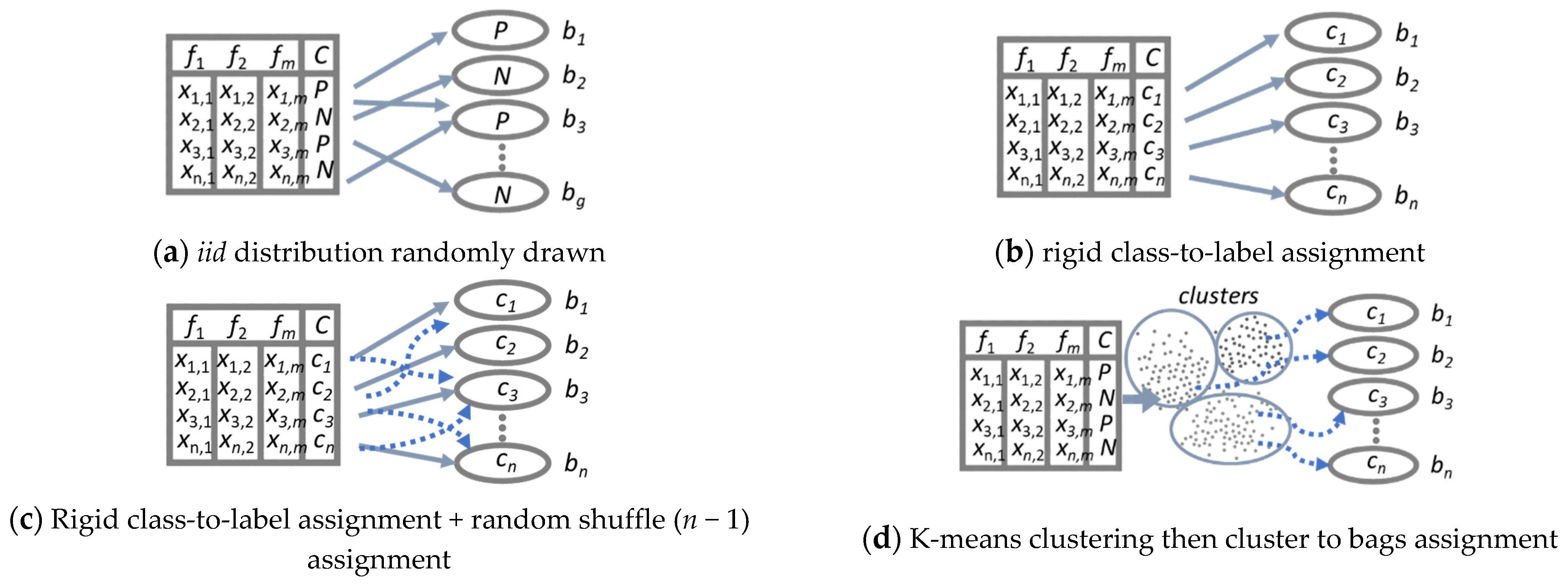
Figure 3 shows illustrations of several possible configurations of the subspace expansion process, which transforms the data instances into bags of data instances. Each configuration can be conducted by different ways of conversion, which could be chosen arbitrarily by the user, such as (a) iid distribution randomly drawn, (b) rigid class-to-label assignment, (c) rigid class-to-label assignment + random shuffle (n − 1) assignment, and (d) K-means clustering then cluster to bags assignment, just to name a few.

One known problem about the subspace transformation is the inflation of the data space very largely. In our experiments, using empirical RS data, the number of features at the original data instances has changed from 27 to 46. This high data feature dimensionality has also largely extended the classifier model construction time from 1.03 s originally to 114.48 s for a typical C4.5 decision tree classifier. Increasing the model construction time, the so called model learning time is not desirable in the fast AI application [21]. In this case, the decision making model by the classifier may be used to learn and look for important events on the ground, in the context of real-time and critical applications such as emergency control, military surveillance, rescue, fire-fighting, etc. [22]; the long latency time implies unavailability or missing-out important events during the model refresh (relearning) when concept drift happens or a new land-type is to be learnt [23].

In order to solve this problem, in our newly proposed algorithm, namely EAC–expand and contract, the subspaces will have to be trimmed down using the fast feature selection method. In this case, swarm feature selection wrapped based was adopted to lower down the risen number of features when genetic algorithm and particle swarm optimization search methods were used respectively. This helps compress the expanded features to half. The process diagram for this EAC-IBL method, which in turn is controlled by the evolutionary swarm search hence called evolutionary EAC-IBL, or simply EEAC-IBL, is shown in Figure 4. Those four methods of transformation from data instances to subspaces shown in Figure 3 are classical IBL methods. However, in Figure 4, an improved version of IBL is proposed by the authors. Instead of placing the data instances into the appropriate bags by random, by fixed, or by self-clustering approaches, it is done by a fast evaluator powered by evolutionary search, so called an optimizer, which selects the best set of instances and matches them to a subspace with respect to the maximum entropy gain. The conversion of data instances to subspaces is by maximum likelihood optimization, implemented by a one-class decision tree. The decision tree of all +ve data are placed to +ve bag b₁. All other bags contain −ve data are b₂, b₃, … b_n.

As a methodology, EEAC-IBL could be applied to other pattern recognition domains where the data are fuzzy and ambiguous in nature. The workflow that is depicted by Figure 4 works as the following three steps. It also serves as a summary of this section where the mathematics basis about this approach is defined.

Step 1. Expand by propositionalizing the original data instances into bags: The space of the original data instances is heuristically partitioned into regions and measuring the occupancy. Data instances are then bagged up. By doing this, the distribution of instances in each bag is known in instance space.

Propositionalization starts by checking (counting the attribute values) how many data instances of a bag should belong to each region. In the partition, for each region there exists exactly one attribute. Hence the propositionalization can become more accurate and holds more information, when compared to relying on the attribute values’ statistics (mean and standard deviation) in a bag. The regions are partitioned using a simple C4.5 decision tree—firstly the data instances are merged to a compact dataset from all the bags, replacing the data class label information by each bag’s class label. Using information gain as a quality indicator, a decision tree is inferred from the compact dataset until maturity. The nodes at the tree branches inherently separate the data space into regions. The occupancy counts are then known, and they indicate at which regions this data instance belongs to, for each instance.

By the concept of bags of instances, the knowledge of labels in the training data is not needed to be precisely known. This ambiguity allows a learning algorithm to exploit more thoroughly the relations between the attributes values and the labels without using the deterministic relations. By the end of this step, bags are generated in which there are unlabeled instances, each bag is labeled with a target class value. For example, a bag is positively labeled as forest type A, if there exists one or more instances in that bag that came from forest type A; the bag is negatively labeled as forest type A, if all the instances inside this bag are free from forest type A label. However, a negatively labeled bag of forest type A may be positively labeled as another forest type.

Step 2. Contract by bag selection using a fast classifier and evolutionary search: In this intermediate step, the number of bags is to be shrunk. The objective of machine learning over bags instead of labeled data instances directly is to predict the labels of unseen bags, which encapsulate the unseen data. Assuming the unseen data would have the same attributes as the training data, the unseen data will have to go through the same preprocessing process too.

In this step, quick bag selection is done like feature selection. A fast classifier is used as an evaluator, which sieves redundant bags keeping only the significant bags. Candidate subset of bags are passed to the fast classifier to obtain an outcome with the highest accuracy. This is a typical combinatorial search problem; evolutionary search methods are applied for finding such optimal candidate subset of bags.

Step 3. Pattern recognition: in this final step, a data stream mining classifier is used right after the above two pre-processing steps, for inducing a prediction model for pattern recognition of the RS forest type.

4. Experiment

For validating the efficacy of the proposed EEAC-IBL model, an empirical dataset that represent a typical scenario of land-type classification was used in the data stream mining experiment. The dataset [24], which represents a case of ASTER satellite remote imaging in land-type image classification, is donated by Johnson et al. of the Institute for Global Environmental Strategies, Japan. The data are results of ASTER satellite imaging, which are formatted by the IR wavelengths representing the spectral characteristics of the objects (which are various Japanese forests). The forests are taken as land-types, which mixed with some formations of land (soils) and canopies of cypress trees—there are four types of forests namely Hinoki, Sugi, deciduous, and non-forest as shown in Figure 5. When the RS imagery data were used to infer up a classification model, it predicts the membership of which land-type the new image belongs to. As the ASTER satellite imaging scans across the land, different types of forests were detected [25]. The image classification has certain accuracy and confidence pertaining to the classification model in use [26].

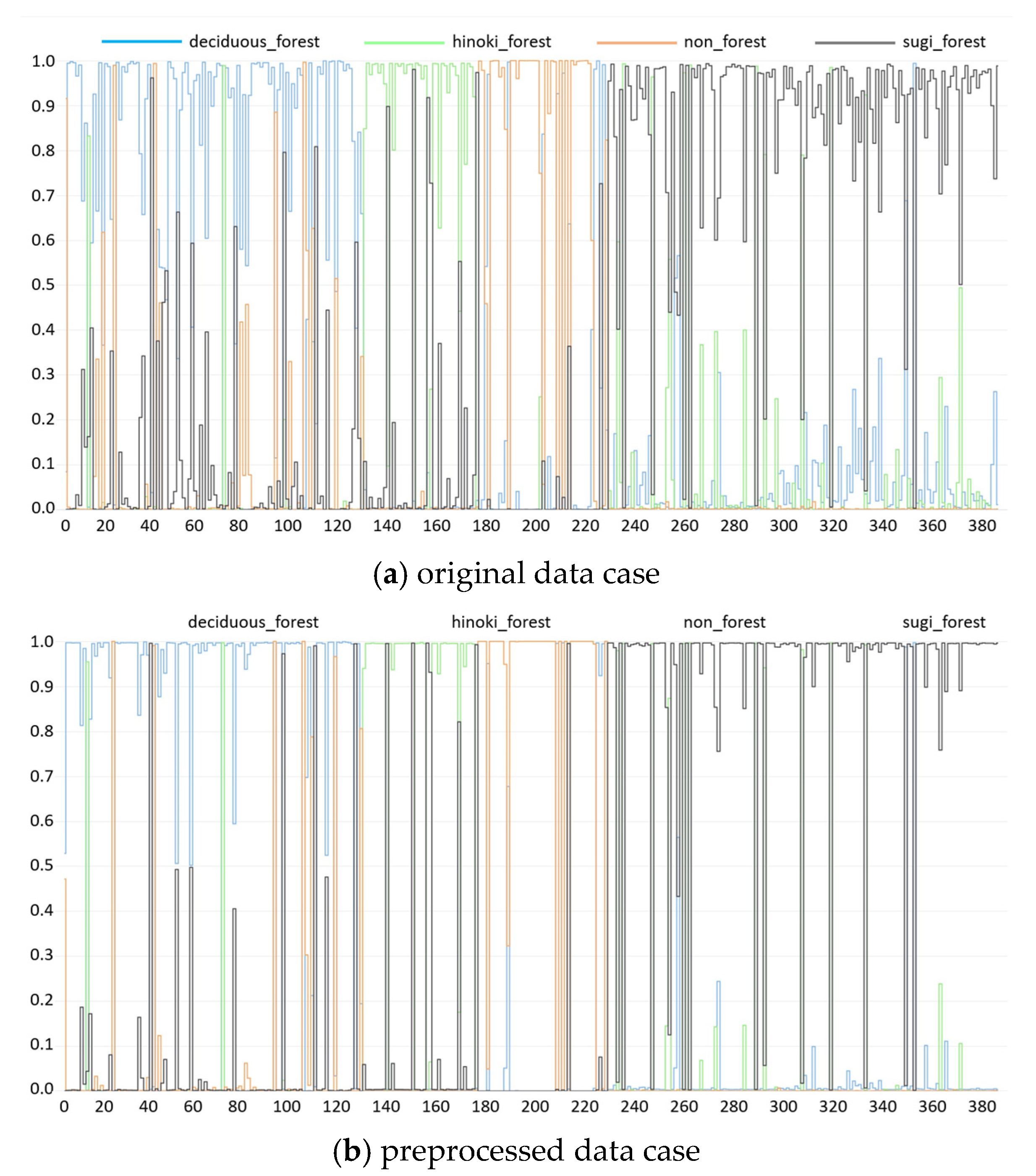
As a proof-of-concept regarding the effect of the preprocessing method, preliminarily a simple data analysis was conducted by using EEAC-IBL over the ASTER satellite data. The original dataset and the preprocessed dataset are loaded into a simple decision tree classifier for full-dataset training, the accuracy of the prediction, which is normalized between 0 and 1, was measured. Figure 6 shows two series of accuracy outputs of several predicted forest types over the axis of abscissas. Two cases are demonstrated with respect to the degree of distinction between different classes of landscapes: in case 6(a) there were no preprocessed over the ASTER data; in case 6(b) the ASTER data was preprocessed using EEAC-IBL method. After the data was preprocessed, the output classes in the form of different colors became more distinctive in case 6(b) as compared to case 6(a) where there are many overlaps and ambiguities among the classes.

The experimentation is designed with the aim of testing and comparing the proposed EEAC-IBL algorithm with a number of variants including the original method using just C4.5 [27] as a classifier to classify land-types into predefined classes based on the spectral values. The simulation platform is a Java-based benchmarking software called Massive Online Analysis (MOA) [28] from Waikato University, New Zealand. MOA simulates a data stream mining environment where the multivariate data stream that has up to 28 features for the original and up to 46 features after being converted, the data instances into subspaces is continuously loading into EEAC-IBL and a one-pass online learner, for learning and refreshing up a classification model incrementally. A sliding window of size 1000 was used, which delivered fresh data for testing and training repeatedly, 1000 data instances at a time. The online algorithm is the Hoeffding Tree [29] sometimes known as a very fast decision tree (VFDT) [30], which is a classical classifier in data stream mining. VFDT is a well-established classifier for data stream mining. It is chosen here as the main supervised learning model for inducing an online learner for the RS pattern recognition. It is known to be fast and lightweight, suitable for real-time machine learning application. Hence it is an appropriate choice for coupling with the EEAC-IBL preprocessing model, which is the proposed contribution in this paper.

The performance criteria under observation are accuracy, Kappa (which measures how much the model can be generalized with new unseen data), memory cost, and time cost. Accuracy and Kappa concerns about how sharp and useful the incremental classifier is, in machine learning for RS image recognition; the memory and time costs are associated with the applicability of the model pertaining to hardware embedding implementation where memory size is desired to be kept as compact as possible, and the data analysis speed in terms of time consumption should be fast enough especially for real-time applications. The software program is version 2014.11, which is a stable version that comes with a GNU General Public License. The hardware platform on which the experimentation was run is a CPU with configuration of Intel Core i7-1065G7 CPU @ 1.3 GHz, 8 Gb RAM and 64-bit OS Windows 10, 2019.

The experimentation results in terms of the four performance criteria from MOA are tabulated in

Table 1. Accuracy of the Hoeffding tree model coupled with ten preprocessing algorithms.

	Original	cfs-bf	cfs-grds	cfs-PSO	cfs-GA	Symmetry-FCBF	EAC	EAC-bf	EAC-GA	EAC-PSO
Max	46.2087	46.2042	46.2042	48.0437	46.0639	47.4147	54.5202	54.5202	54.5202	54.5202
Mean	82.8557	82.8467	82.8467	86.5256	82.5660	85.2675	99.4786	99.4786	99.4786	99.4786
Min	9.5618	9.5618	9.5618	9.5618	9.5618	9.5618	9.5618	9.5618	9.5618	9.5618

,

Table 2. Kappa of the Hoeffding tree model coupled with ten preprocessing algorithms.

	Original	cfs-bf	cfs-grds	cfs-PSO	cfs-GA	Symmetry-FCBF	EAC	EAC-bf	EAC-GA	EAC-PSO
Max	36.3508	36.0546	36.0546	39.2934	29.2983	38.3164	29.2983	29.2983	29.2983	29.2983
Mean	63.9743	63.3819	63.3819	69.8596	49.8693	67.9056	49.8693	49.8693	49.8693	49.8693
Min	8.7273	8.7273	8.7273	8.7273	8.7273	8.7273	8.7273	8.7273	8.7273	8.7273

,

Table 3. Time consumption (in seconds) of the Hoeffding tree model coupled with ten preprocessing algorithms.

	Original	cfs-bf	cfs-grds	cfs-PSO	cfs-GA	Symmetry-FCBF	EAC	EAC-bf	EAC-GA	EAC-PSO
Max	0.1016	0.0547	0.0625	0.0547	0.0703	0.0313	0.0625	0.0156	0.0313	0.0156
Mean	0.1875	0.1094	0.1250	0.0938	0.1250	0.0625	0.1094	0.0313	0.0469	0.0313
Min	0.0156	0.0000	0.0000	0.0156	0.0156	0.0000	0.0156	0.0000	0.0156	0.0000

and

Table 4. Memory consumption (in bytes) of the Hoeffding tree model coupled with ten preprocessing algorithms.

	Original	cfs-bf	cfs-grds	cfs-PSO	cfs-GA	Symmetry-FCBF	EAC	EAC-bf	EAC-GA	EAC-PSO
Max	4.04 × 10−10	1.30 × 10−10	1.50 × 10−10	9.60 × 10−11	1.65 × 10−10	2.99 × 10−11	3.22 × 10−10	1.34 × 10−11	5.85 × 10−11	3.98 × 10−11
Mean	7.60 × 10−10	2.61 × 10−10	3.00 × 10−10	1.70 × 10−10	3.00 × 10−10	5.99 × 10−11	5.63 × 10−10	2.68 × 10−11	8.78 × 10−11	7.97 × 10−11
Min	4.87 × 10−11	0.00 × 10+00	0.00 × 10+00	2.22 × 10−11	2.93 × 10−11	0.00 × 10+00	8.04 × 10−11	0.00 × 10+00	2.93 × 10−11	0.00 × 10+00

as follow. The maximum mean and minimum of each performance indicators values were measured and reported over a million data records of data stream mining. The results of these four tables had significance in data stream mining. Each set of results were grouped as a minimum, maximum, and average. They represent how well the data stream mining operation has been ongoing as the RS functions. Due to the “test-then-train” strategy in data stream mining, the performance fluctuates depending on the current efficacy of the model and the characteristics of the incoming data. The results tabulated in the four tables are those that have been averaged over the whole testing period, with the peak performance recorded as maximum and the lowest performance value recorded as minimum.

The evaluation mechanism is prequential, meaning the model is refreshed progressively from the beginning to the end. Each time a window load of fresh data is subject to the model for testing then training. In general, the performance improves over time when more and more data is being seen. Each data arrives as one pass, stored briefly in the window buffer, and discard without further storage. This way, the processing load is relieved especially in distributed environment such as Cloud computing without the need of storing up all the historical data, which are merely sensor data measurement, too massive and not worth to keep for a long term archive.

However, the model serves as a real-time watch dog, being able to recognize the activities from the patterns of the sensor data. The efficacy of the model improves in time, as training progresses. During supervised training, the model would have seen an increasing amount of training samples that come continuously from the data feed. Eventually the model matures. A concept is well established from the underlying relations between inputs and outputs, after the model has observed sufficient samples from the training data.

Twelve configurations of algorithms are being tested comparatively. One type of configuration is a standard configuration with the use of raw data. The second type of configuration is combinations of standard preprocessing using correlation-based feature selection, coupled with best first search, greedy-step search, particle-swarm-optimization (PSO) search, and genetic algorithm (GA) search [31]. Other variants of standard configurations embrace a standard and popular feature selection called the symmetrical uncertainty measure with a fast correlation based filter (FCBF) search [32] was tested. The other configurations tap on the use of EAC that is based on instance-based learning where data instances were converted to the subspace. Enhanced EAC methods such as EAC using correlation-based feature selection with best first, and EAC with evolutionary swarm searches of PSO and GA are in this type of configurations too.

Thereafter, the acronyms depicting the twelve versions of preprocessing in the order of the above-mentioned names are original, cfs-bf (that stands for correlation feature selection coupled with best first search), cfs-grds (that stands for correlation feature selection coupled with greedy-search), cfs-PSO, cfs-GA, symmetry-FCBF, EAC, EAC-bf, EAC-GA, and EAC-PSO.

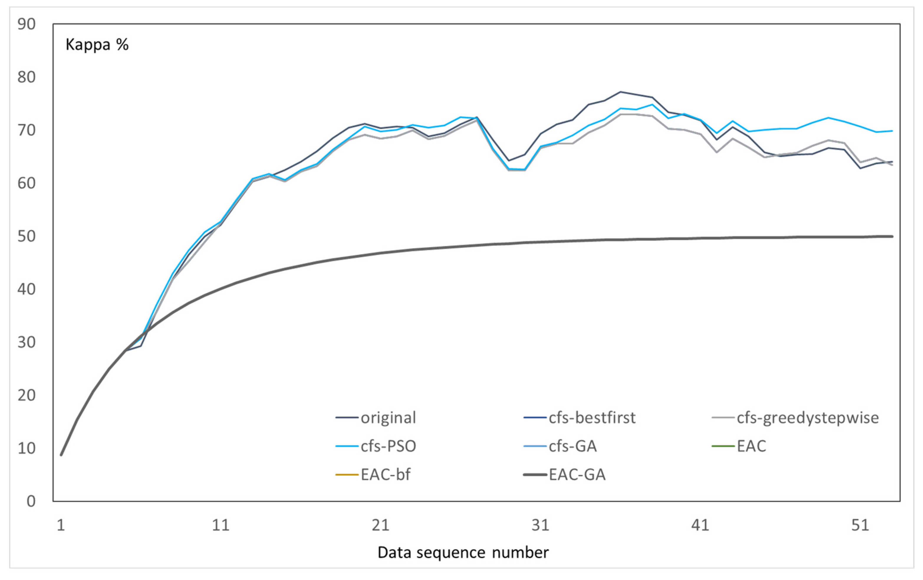
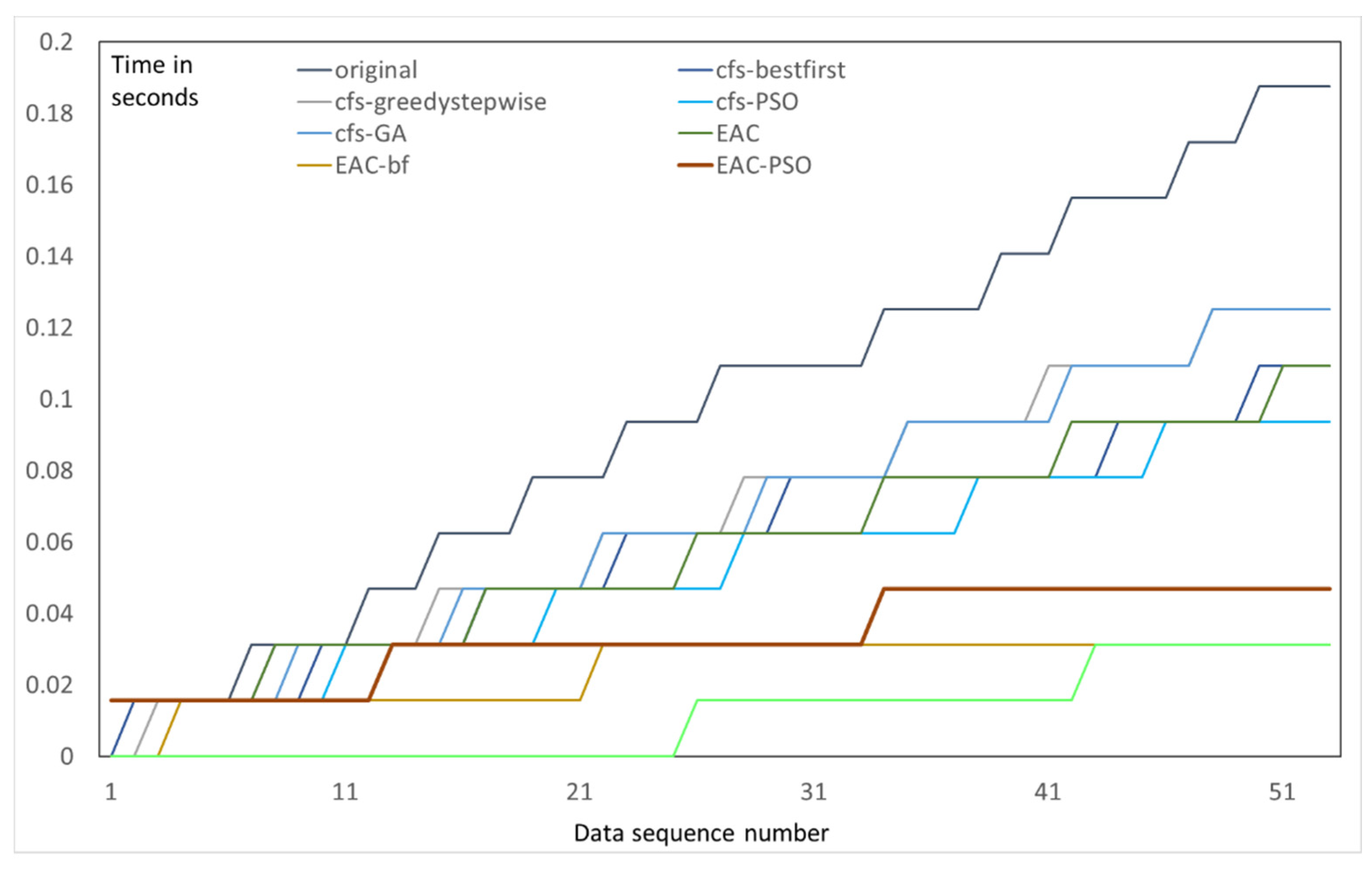
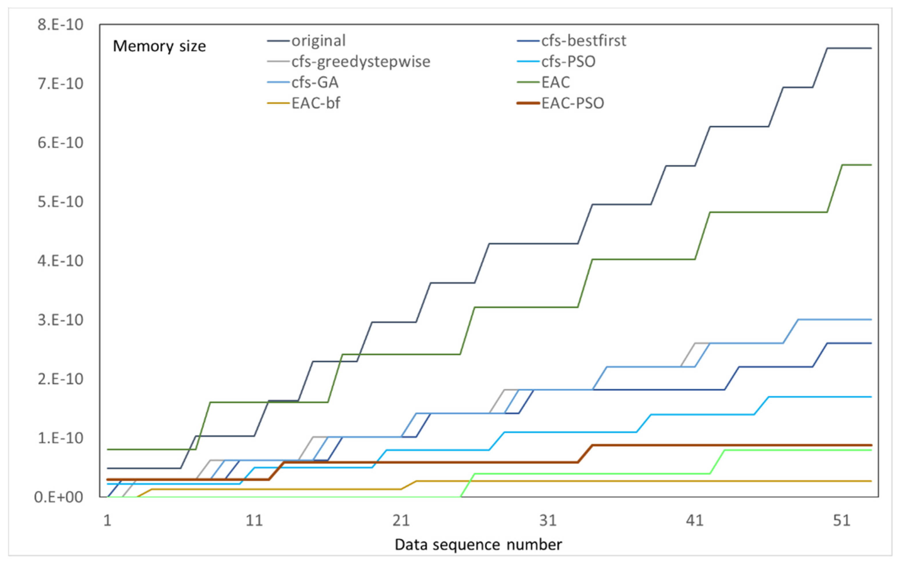
The base learner for the RS image recognition is the Hoeffding tree in the MOA environment. The visualizations of the performance results were charted as curve graphs showing the change of performance indicator value over the data stream, are shown in Figure 7: Accuracy, Figure 8: Kappa, Figure 9: Time, and Figure 10: Memory. Accuracy is defined by the number of correctly classified cases with respect to each one of the multiclasses over the total number of cases. Kappa is measured by how well a trained model can be generalized for many unseen datasets. These two are the major performance indicators for most of the classification scenarios. However, for real-time classification, additional performance indicators such as the model refresh time and amount of memory consumed in each round of update are taken into consideration.

The accuracy measure is important because a classifier must be able to correctly recognize the correct land-type in the field [33]. The experiment results show that EAC was the best, with a final level of accuracy at 99.48% in comparison to the original form at 82.86% in Table 1. EAC, which is based on instance-based learning with subspace and such, managed to overcome the data ambiguity problem rooted in the RF streaming data from measuring the spectral values of a field-of-vision of an area that moves over a land, which is never easy to attain high precision. However, it is shown also that in general both evolutionary swarm search methods could cut down the memory requirement, time, and the total size of the subspaces while achieving relatively good mean levels of accuracy.

As an incremental learner, it is shown that in Figure 7 and Figure 8 that the longer the data stream mining runs, the performance rises and approaches an exponential curve towards some steady-state maximum performance. However, in the data stream mode, EAC attained the best performance and its variants show no difference in changes of the level of performance. This implies EAC is good enough in terms of feature engineering.

There are not too many features, 28 in the original dataset and 17 and 23 under EAC-PSO and EAC-GA respectively. Each time there is only a window of data made available for testing and training. As a result, the maximum accuracy is limited or capped at a certain accuracy percentage. The shortage of available data makes the accuracy hardly improve further. However, on the other hand, when the same simulation is tested in the traditional data mining environment, where all the training and testing data are available, there are apparent differences in which feature selection methods were being used.

Table 5. Comparison of performance of traditional decision tree model coupled with ten preprocessing algorithms.

Methods	Accuracy	Kappa	True Positive	False Positive	Precision	Recall	F-Score
original	85.8509	0.8011	0.859	0.061	0.86	0.859	0.858
cfs-bf	85.6597	0.7992	0.857	0.06	0.857	0.857	0.857
cfs-grds	85.6597	0.7992	0.857	0.06	0.857	0.857	0.857
cfs-PSO	85.4685	0.7964	0.855	0.061	0.855	0.855	0.855
cfs-GA	84.8948	0.7884	0.849	0.062	0.85	0.849	0.849
symmetry-FCBF	86.2333	0.8075	0.862	0.057	0.863	0.862	0.862
EAC	93.499	0.9091	0.935	0.027	0.935	0.935	0.935
EAC-bf	88.3365	0.836	0.883	0.054	0.892	0.883	0.884
EAC-GA	92.543	0.8955	0.925	0.029	0.931	0.925	0.925
EAC-PSO	92.9254	0.9012	0.929	0.028	0.931	0.929	0.93

shows the performance results of data mining where all the RS data are available. The performance results of the EAC variants appeared to be more superior.

The performance results in Kappa show approximately the same trends as those in Table 2 and Figure 8. However, it is interesting to note that the Kappa performance for those standard methods with swarm search and other standard feature selection methods cannot sustain themselves, the kappa of the EAC family of methods fall generally below the standard methods. This indicates the classifier model trained by the standard methods even using swarm search are unable to generalize its RS image recognition ability when totally new data are to be applied. For example, a model could be trained well given the same set of training and testing datasets. However, after trained, when unseen datasets are tested on, Kappa, which sometimes is taken as a reliability indicator [34], tells us how well the model would still be useful upon testing with unseen datasets. The higher the Kappa the better chances that testing with new data will still be good.

Finally, the time and memory costs comparison, as shown in Table 3 and Table 4 and Figure 9 and Figure 10, they all demonstrate that the rate of increase in time and memory were scaling up linearly. This is important implying that the methods tested here will not have any data or time explosion; the two costs reasonably went up as more data were tested accumulatively. In short, the proposed EAC family of algorithms did have an edge in performance advantage, solving the data ambiguity problem at sensor data for RS image recognition.

5. Conclusions

Remote sensing had broad application domains such as remote surveillance and critical event monitoring. Often real-time surveillance applications [35,36] have urgent constraints that require fast data analytics in analyzing the situations quickly and accurately. Land scanning by high resolution imaging of satellite generates a large amount of real-time data [37,38], which is continuous and dynamic—situations and landscapes change.

The sheer volume and real-time requirements of remote sensing pose a great machine learning challenge in finding the most suitable data mining algorithm. Besides accuracy and robustness, there are other performance requirements associated with RS image recognition over long distance transmission—time and memory costs. The machine learning must be fast for timely availability and efficacy, at the same time it is desired to keep the model compact in memory. For example, the logics could be built into a small chip or microprocessor in the space equipment, as an embedded solution. An alternatively new machine learning methodology was proposed in this paper. In lieu of traditional machine learning model, data stream mining model was used, for fast and adaptive online learning. At the same time, a novel preprocessing mechanism was proposed called evolutionary expand-and-contract instance-based learning algorithm (EEAC-IBL).

By the EEAC-IBL algorithm, the sensing data from a satellite collected in a form of multivariate data stream is first expanded into many subspaces, then the subspaces, which are corresponding to the characteristics of the features, are selected and compressed into a significant feature subset. Instead of deterministic, the selection process is stochastic that is empowered by evolutionary optimization in finding the best subgroup. Then the model learning is carried out on the fly using data stream mining for learning concepts from the new data for land-type recognition. The proposed EEAC-IBL taps on the advantages of the multiple instance learning mechanism, which is suitable for learning from fuzzy data concepts where precise feature selection is not applicable because of concept drifts along the data stream over time. Inherent from the merits of the stochastic approximation method, EEAC-IBL is fast and accurate. More importantly, its learning ability is adaptive over data streams; our simulation experiments show that EEAC-IBL is able to improve its accuracy over time compared to the traditional machine learning method in a simulated land-type image recognition application. Based on a decision tree learner as a benchmark, a mean accuracy is only attained at 85.85% without any preprocessing. This performance is not improved at all using the popular correlation-based feature selection. Using EAC alone, the performance was boosted to 93.5% at the cost of consuming a lot of memory for using subspace partitioning and a slightly long run-time. This shortcoming of EAC was alleviated by evolutionary and stochastic optimization mechanism, which evolved to EEAC-IBL, which shortens the time and memory requirement. The compromised accuracy of EEAC-IBL reached at 92.93% balancing the objectives of maximizing accuracy, while minimizing time and memory. The results give hope that this new EEAC-IBL method could be a promising adaptive machine learning technique for ASTER imaging, expanding its potentials for many critical applications, in which the data streams are being processed fast with concept drift. The proposed method was based on the multiple instance learning. Different feature selection methods were compared in the experimental section. As future work, the state-of-the-art feature selection methods outside of the multiple instance learning would be used in the comparative experimentation as well.