Abstract
The standing stock of phytoplankton carbon is a basic and essential property for understanding oceanic ecosystems, biogeochemical cycles, and regional climates. However, current related algorithms mainly focus on remote-sensed application, which cannot describe the vertical profile of phytoplankton carbon throughout the whole euphotic zone. In this study, we modified a previous absorption-based bio-optical algorithm to acquire vertical variabilities of the total and size-partitioned phytoplankton carbon based on field data from the South China Sea (SCS). The mean absolute errors and the biases between estimated and field picophytoplankton carbon were <2.14 and 0.6–2.0, respectively. The results showed that the vertical profile of total phytoplankton carbon displayed a Gaussian distribution in the stratified SCS basin. The picophytoplankton carbon was always the fundamental component of the total phytoplankton carbon within the whole euphotic zone. The dominant picophytoplankton species changed from Synechococcus-like cyanobacteria at the sea surface to pico-sized haptophytes at the phytoplankton carbon maximum layer. The strong covariation between total phytoplankton carbon and chlorophyll-a concentration suggested that they can be converted into each other through an accurate carbon-to-chlorophyll ratio in the open SCS. These results provide essential information that can be used to decipher the three-dimensional structure of total and size-partitioned phytoplankton carbon in the open SCS.
1. Introduction
Marine phytoplankton is a key component of global carbon cycling, accounting for about half (~50 Gt C) of global annual primary production through oxygenic photosynthesis [1,2]. Knowledge of the standing stock and dynamics of marine phytoplankton is crucial for understanding the global carbon cycle and climate. In recent decades, the most commonly used indicator of phytoplankton biomass has been the total chlorophyll-a concentration (Chla, in mg m−3) [3,4]. However, in the “photoacclimation regime” [5], the first order changes in Chla are due to intracellular pigment variation resulting from light and nutrient variations [6], thus Chla cannot provide a full description of the state of the ecosystem under such a regime [7]. Instead of Chla, total phytoplankton carbon biomass (C, in mg m−3) is the parameter more directly related to the carbon cycle, biogeochemical cycles, and climate [7,8]. Accurate estimation of C provides a means to observe the standing stocks of phytoplankton and their response to environmental variability [9]. However, direct measurement of C remains challenging due to the inability to isolate C from the other particulate forms of carbon in seawater (e.g., zooplankton, detritus, and bacteria) [9]. Consequently, estimating C from other easier to measure proxies, such as optical parameters, maybe an easier approach.
With the development of observed technology, many bio-optical models have been built to derive Chla as well as chlorophyll-a concentrations in three size classes (e.g., [10,11,12]). In terms of C, several bio-optical models for C estimation have been proposed recently as well [6,7,13,14,15]. C is an important component of particulate organic carbon (POC, in mg m−3) in the vast oceans. Sathyendranath et al. [14] developed a simple conceptual model to calculate C from Chla based on the assumption that at any given Chla, the lowest POC observed represents the C associated with that Chla. C can also be computed through Chla or POC by assuming a C-to-Chla () or C-to-POC ratio. Based on the assumption that the particles contributing to particulate backscattering coefficients (bbp(), in m−1) are composed of a stable non-algal “background” component and a second component including phytoplankton and other particles that co-vary with phytoplankton, Behrenfeld et al. [6] subtracted the non-algal particulate backscattering coefficients (bnap(), in m−1) based on the relationship between bbp() and Chla and then calculated C through the remaining bbp() based on a simple scaling factor. The simple scaling factor was derived such that the resulting C was ~25 to 40% of POC and the average value was within the range observed in laboratory studies [16]. However, bnap() varies in different oceanic regions (e.g., [17,18]). Bellacicco et al. [17] reported that using a constant bnap() to estimate C will lead to a 50% overestimation in satellite-based global C estimates with respect to the results based on varied bnap() in different regions. Meanwhile, based on Biogeochemical-Argo data, Bellacicco et al. [18] also reported that bnap() in the surface layer increased from Southern to Northern Hemisphere, and bnap() was the main contributor to bbp() in the surface oligotrophic waters while the contribution of bnap() decreased in the surface layer of most productive areas. Besides, variabilities in particle size distributions also lead to differences in backscattering per unit carbon biomass due to different scattering efficiencies [7,19]. Accordingly, Kostadinov et al. [19] built a bbp() model to estimate particle size distributions (power-law distribution), and later Kostadinov et al. [7] combined the allometric relationships to compute C and size-partitioned phytoplankton carbon biomass based on the assumption that the value of C-to-POC ratio was 30%. However, the uncertainty in C estimation due to contribution of other types of non-algal particles to bbp() still exists. To avoid this problem, Roy et al. [15] developed a semi-analytical algorithm (R17) to calculate C and size-partitioned phytoplankton carbon that is based on the specific absorption coefficient of phytoplankton (which is defined as the ratio of the absorption coefficient of phytoplankton to Chla, (), in m2 mg−1), which is directly related to phytoplankton. These advances in C estimation algorithms provide effective means to estimate C from in situ to remote platforms.
The South China Sea (SCS) is the largest trophic marginal sea in the northwestern Pacific Ocean, and it plays important roles in regulating the regional carbon cycle and climate due to its vast area and volume [20,21]. Macronutrient concentrations in the central basin of SCS are below the detection limit, which suggest the SCS basin is oligotrophic [20,22,23]. Because it is oligotrophic, the open SCS is dominated by picophytoplankton, namely Prochlorococcus, Synechococcus, and picoeukaryotes [20]. Previous studies of the phytoplankton biomass variation in the SCS have been based mostly on Chla. However, photoacclimation is an important factor controlling variability of the Chla in the open SCS [21], and this process limits our understanding of the real distribution and variation of the phytoplankton pool as well as the biological carbon pump in the SCS. Therefore, in this study we estimated the vertical standing stocks of phytoplankton from the perspective of carbon mass rather than Chla. It provides another perspective for studying the distribution and variation of phytoplankton biomass in the SCS.
To avoid using preset values of C:POC and effects of the non-algal particles, we chose the absorption-based carbon algorithm to estimate the phytoplankton carbon concentration in the SCS. First, we modified the algorithm described by Roy et al. [15] using the in situ absorption coefficient of phytoplankton [aph(), in m−1] and Chla dataset, and then we applied it to the non-watery beam absorption [apg(), in m−1] that was measured by an absorption-and-attenuation-meter (AC-S, WET Lab Inc., Philomath, OR, USA). The algorithm-derived picophytoplankton carbon values were validated by in situ measurements of picophytoplankton carbon. We then analyzed the characteristics of the vertical profiles of total and size-partitioned phytoplankton carbon in the open SCS basin. To ease the conversion between C and Chla, we analyzed the regional relationships between C and Chla as well. Table 1 shows the main abbreviations used in this study. This study provides important information for studying phytoplankton dynamics and the regional carbon cycle and climate in the SCS.

Table 1.
The main abbreviations used in this study.
2. Materials and Methods
2.1. Study Area and Field Sampling
The SCS extends from 3 S to 23 N and from 99 E to 121 E, and it includes two wide shallow shelves in the northern and southern parts and a large deep basin in between [24]. The upper ocean layer of the SCS is mainly affected by eastern Asian monsoons [25], periodic typhoons, Kuroshio intrusions, and fresh water inflow [26]. The circulation of the SCS is cyclonic in winter but anticyclonic in summer [24]. The open SCS is generally stratified, warm, and oligotrophic, with low phytoplankton biomass [20,21]. The vertical Chla is generally characterized by a pronounced deep maximum at 60–100 m in the open SCS [21,27,28,29].
Three cruises were carried out in the SCS to collect bio-optical parameters: 27 June to 17 July 2015 (cruise 2015), 3–23 September 2016 (cruise 2016), and 1–22 October 2017 (cruise 2017). The bio-optical parameters (absorption coefficient of phytoplankton [aph(), in m−1], Chla, picophytoplankton carbon biomass, and POC) were obtained at four depths (0 or 5, 25, 50, and 75 m). POC data were only collected during cruises 2015 and 2017. Additionally, an AC-S instrument was used to measure the vertical profiles of apg() during cruises 2015 and 2016. A simultaneously seabird conductivity-temperature-depth (CTD) was used to obtain the profiles of temperature and salinity. The AC-S and CTD were assembled in a cage to measure the optical and hydrographic parameters from surface to about 120 m. Figure 1 shows the locations of the sampling stations.
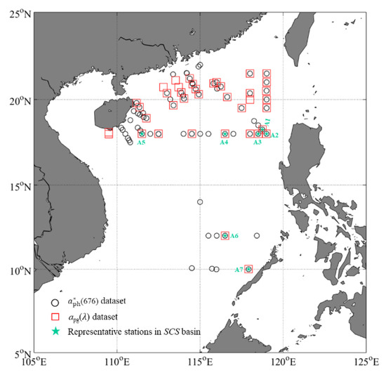
Figure 1.
Locations of stations in the SCS. The black hollow circles represent the stations for the (676) dataset. The red squares represent the stations for the apg() dataset. The green stars represent the warm and oligotrophic stations (>1000 m) with strong stratification in the SCS basin.
2.2. Field in Situ Data
2.2.1. Measurement of aph() and Calculation of ()
To obtain aph() from 350 to 750 nm, 0.5–3.0 L of seawater, depending on the station, were filtered through a 25 mm glass fiber filter (Whatman, GF/F, Maidstone, UK) under low vacuum conditions. Because our laboratory bought a new spectrophotometer in 2016, the measurements of aph() for cruise 2015 were made using a Shimadzu UV-2550 spectrophotometer (Kyoto, Japan), and those for cruises 2016 and 2017 were made using a PerkinElmer Lambda 650S spectrophotometer (Waltham, MA, USA) based on the quantitative filtered technique (QFT). The reference blank was a clear filter that was presoaked in pure water. First, the absorption coefficient of total particles [ap(), in m−1] was measured. Then the absorption coefficient of non-algal particles [anap(), in m−1] was measured after soaking the filters in methanol for 90–180 min to remove phytoplankton pigments. All measurements were corrected for the background signals by subtracting the absorption values at 750 nm over the whole wavelength [30]. Corrections for pathlength amplification were made according to Stramski et al. [31]. Finally, aph() was calculated as the difference between ap() and anap(). The values of () were calculated by dividing aph() by the corresponding field in situ Chla.
2.2.2. Measurement of apg()
The vertical profiles of apg() were measured using a 25 cm pathlength AC-S with 82 wavebands from 401.6 to 744.1 nm. Pure water was used to calibrate the drift of the AC-S instrument and as the reference blank before cruises. To avoid the influence of bubble, the AC-S was lowered below the water’s surface for ~5 min to warm up, and after the warm up period, the AC-S was steadily lowered through the water column to collect data. Before data correction, the software “WET Labs Archive File Processing” (WAP) was used to merge the AC-S and CTD data. The corrections for temperature and salinity effects were made using contemporaneously recorded CTD data [32]. All measurements were corrected for scattering by setting the absorption values as zero around the infrared wavelengths [33].
2.2.3. Pigment Concentration Measurement and Determination of Dominant Phytoplankton Species
The values of Chla were measured in two ways: fluorescence method and high-performance liquid chromatography (HPLC). For the fluorescence method, 0.5–1.0 L of seawater were filtered through a 25 mm Whatman GF/F filter with 0.7 m pore size to obtain Chla. In the laboratory, filters were soaked in acetone in the dark for 24 h to extract the chlorophyll a. Then, Chla was measured using a Turner Design 10 fluorometer (Sunnyvale, CA, USA) [34]. For HPLC, 2.5–10 L of seawater were filtered through 25 mm or 47 mm Whatman GF/F filters with 0.7 m pore size and stored in liquid nitrogen until analysis in the laboratory. For surface samples (0 or 5 m), 8–10 L of seawater were filtered on the 47 mm Whatman GF/F filters. As for the samples at 25, 50 and 75 m, 2.5–5 L of seawater were filtered on the 25 mm Whatman GF/F filters. The collection of HPLC samples was generally according to the Joint Global Ocean Flux Study (JGOFS) protocols [35]. See Vidussi et al. [36] for analysis details. The HPLC data were also used to calculate the size-partitioned Chla according to the method in Brewin et al. [10].
Determination of dominant phytoplankton species was made according to the criteria in Table 4 from Alvain et al. [37] and this method was based on the relative concentrations of main biomarkers of the Prochlorococcus, Synechococcus-like cyanobacteria, haptophytes, dinoflagellates and diatoms of the water samples to determine the dominate phytoplankton species.
2.2.4. Picophytoplankton Carbon Biomass and POC Measurements
To measure picophytoplankton carbon biomass, seawater samples were filtered through a 20 μm sieve and preserved with formaldehyde (2% final concentration) for picophytoplankton cell (Prochlorococcus, Synechococcus and autotrophic picoeukaryotes) counting. The samples were freeze-trapped in liquid nitrogen after 15 min of standing in the dark. Measurements of picophytoplankton cell abundances were made using a BD FACSCanto II flow cytometer (Franklin Lakes, NJ, USA). Before measurement, velocity correction was carried out according to Marie et al. [38]. According to the scatterplots of different fluorescence or side scattering, cell abundances of the three picophytoplankton categories were determined. Carbon contents of the three picophytoplankton categories were estimated from cell abundances by assuming conversion factors of 17.6 fg C cell−1 for Prochlorococcus, 74.55 fg C cell−1 for Synechococcus, and 779.9 fg C cell−1 for picoeukaryotes respectively [summer-winter averaged values in Chen et al. [20]]. The sum of the carbon contents of the three picophytoplankton types is defined as the field picophytoplankton carbon biomass.
For POC measurement, 0.5–4.0 L seawater was filtered onto a pre-combusted (450 °C for 5 h) 25 mm Whatman GF/F fiberglass filter and then stored in a −20 °C fridge. The method of POC measurements was generally consistent with the Joint Global Ocean Flux Study (JGOFS) protocols [35,39]. In the laboratory, the POC samples were dried at 60 °C for 8 h and then acidified by hydrochloric acid fumigation to remove the inorganic carbon. Finally, the filters were dried again and the POC concentrations were measured using a Vario UNICUBE elemental analyzer (Elementar Analysensysteme GmbH, Langenselbold, Germany).
2.3. Derived Data
2.3.1. Physical and Biogeochemical Layer Depths (Layers) of the Water Column
The mixed layer depth (MLD, in m) was estimated based on a threshold potential density difference (0.03 kg m−3) from a near-surface value (at 10 m) [21]. The depth of the euphotic zone (Zeu, in m) was estimated based on average Chla within 10 m (Chlasurf, in mg m−3) as Zeu = 35 Chlasurf −0.35 (from Cao et al. (2002) [40]. The depth of 22 °C isotherm (ZT22, in m) was used as the proxy for the nutricline [24]. The C maximum layer (CML) was defined as the layer where a pronounced C maximum appeared in the vertical profile.
2.3.2. Definition of Trophic Categories
The trophic category (for stratified waters) of each station was defined by the value of Chla at 0 or 5 m according to the threshold in Table 3 from Uitz et al. [41]. The trophic level increased sequentially from S1 (the most oligotrophic) to S9 (the most nutritious) in the stratified waters.
2.3.3. Algorithm Performance Metrics
The mean absolute error (MAE), the root mean square (RMSE), and bias between algorithm estimations and field observations were calculated to evaluate the performance of the algorithm [42]:
where n, Cderived, and Cfield represent the number of samples, the estimated products, and field measurements, respectively.
2.4. Phytoplankton Carbon Estimation
Figure 2 shows the flow chart of the phytoplankton carbon estimation. The aph() was first used to validate the phytoplankton carbon model, and then we applied the model to the apg() data to obtain high-resolution vertical distribution profiles of total and size-partitioned phytoplankton carbon in the SCS.
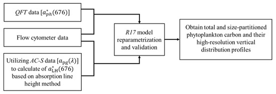
Figure 2.
Flow chart of the regional phytoplankton carbon algorithm reparameterization and application into field data.
2.4.1. Phytoplankton Carbon Estimation Algorithm
The phytoplankton carbon estimation algorithm, R17, uses the aph(676) and Chla as inputs and combines the allometric relationship between phytoplankton cell size and carbon content to calculate total and size-partitioned phytoplankton carbon. A main assumption of R17 is that the phytoplankton size spectrum follows a power-law distribution. In preparation for estimation of C, the exponent of the phytoplankton size spectra () is first computed from (676) using the method described in Roy et al. [12]. The can be computed following Equation (4) in MATLAB using a single-variable bound non-linear-function minimization method based on golden section search and parabolic interpolation [12]:
where (676) on the left-hand side is the observed specific absorption coefficient of cholorophyll-a at 676 nm [43]; (676, D) on the right-hand side is the theoretical value of specific absorption coefficient of chlorophyll-a at 676 nm, which is expressed as a function of the equivalent spherical diameter D of phytoplankton [43]; m is the exponent of the relationship between intracellular Chla (Chlacell, mg m−3) and D (Chlacell = c0D−m), here set as m = 0.06 (dimensionless) and c0 = 3.9 106 (mg Chla m−2.94) [43]; minimum diameter Dmin = 0.2 µm; and maximum diameter Dmax = 50 µm [15].
The allometric relationship between the cellular content of phytoplankton carbon (Ccell) and cell volume (Vcell) for phytoplankton communities was then used to calculate C [44]:
where Vcell is the volume of a phytoplankton cell expressed in µm3, Ccell is expressed in pg C cell−1, and a = 0.54 and b = 0.85 are constants [15]. C within a diameter range [Dmin, Dmax] can then be expressed as:
It should be noted that 10−9 and 1018 are the conversions of units from pg to mg and from m3 to µm3, respectively. The diameter ranges of pico-, nano-, and micro-sizes were set at 0.2–2.0, 2–20, and 20–50 µm, respectively [15]. The carbon biomass of pico- (Cp, in mg m−3), nano- (Cn, in mg m−3), and microphytoplankton (Cm, in mg m−3) was calculated through the product of and Chlai, where i represents pico-, nano-, or microphytoplankton. is expressed as a function of , m, and the upper and lower bounds of diameter of the three size classes. The Chlai was estimated using the Chla and chlorophyll-a fractions of the three size classes (see Roy et al. [12] for details). Finally, the fractions of carbon associated with pico- (Fp), nano- (Fn), and microphytoplankton (Fm) were calculated through Ci and C.
2.4.2. Modification of the Algorithm
The (676) is not necessarily equal to (676), especially in low-Chla conditions [43]. Therefore, (676) values were converted to the corresponding (676) values using an ad-hoc non-linear function [43]:
where = , and = 0.028 m2 (mg Chla) −1 was the maximum numerical value of (676) reported for laboratory cultures, and am was the maximum (676) determined from in situ measurements. To estimate over a realistic range of measured (676), am was set to 0.0226 m2 mg−1 for the (676) dataset; for the apg(λ) dataset, am was set to 0.0128 m2 mg−1. In addition, the upper bounds for (676) were the am values in different datasets, respectively, and the lower bound for (676) was set to 0.007 m2 mg−1.
2.4.3. Application of the Algorithm to apg()
It is not enough to apply R17 to remote sensing data (which only observes the surface distribution) and QFT-(676) data (which only observes the variations at several discrete depths) to obtain a three-dimensional distribution of C, Cp, Cn, and Cm. Thus, we tried to apply the R17 algorithm to apg() data to obtain the high-spatial-resolution vertical profiles of total and size-partitioned phytoplankton carbon. To do this, the values of Chla were first derived using the absorption line height method (ChlaLH, in mg m−3) [45]. The absorption line height at 676 nm [aLH(676), in m−1] was calculated from apg() as follows:
aLH(676) = apg(676) − [0.52 × [apg(700) − apg(650)] + apg(650)].
The ChlaLH was then calculated using aLH(676) based on a regional empirical power-law relationship between field Chla and aLH(676) in the SCS:
ChlaLH = 65.57 × aLH(676)0.96.
The correlation coefficient (R), RMSE, bias, and MAE between field Chla and ChlaLH were 0.88, 0.11 mg m−3, 1.03, and 1.45, respectively (Figure 3). The specific-absorption coefficient of phytoplankton from apg() (, in m2 mg−1) was defined as: (676) = aLH(676)/ChlaLH. Finally, the ChlaLH and (676) were used to estimate the total and size-partitioned phytoplankton carbon.
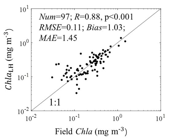
Figure 3.
Relationship between field Chla and ChlaLH. The black line is the 1:1 line. The Num is the number of sample.
3. Results
3.1. Algorithm Validation
To evaluate the applicability of R17, validation of R17 was carried out using field data (both QFT- and AC-S-apg(676) data) from the SCS. Because field C, Cn, and Cm are difficult to obtain, validations were limited to Cp. The field observed Cp for algorithm validation was the product of flow-cytometry-measured picophytoplankton cell abundance and the corresponding carbon conversion coefficient. The field observed Cp was independent of the algorithm-derived Cp. The details of the field observed Cp measurement were in Section 2.2.4.
3.1.1. Validation of Estimations from (676)
Figure 4a shows validation results for estimations from (676). The value of R between field Cp and estimated Cp based on R17 was 0.58 (p < 0.001), and the values of MAE and bias between field Cp and the (676)-derived estimations were 2.14 and 0.62. The scatter points were distributed near the 1:1 line (black line in Figure 4a). Uncertainties in the carbon conversion factors would lead to 2- to 3-fold overestimation of field Cp [46]. The median value of the estimated Cp was lower than that of the default field estimations but higher than those of a 2- or 3-fold overestimations of the field observations (Figure 4b). In addition, the field was calculated as the ratio of field Cp and picophytoplankton chlorophyll-a concentration derived from HPLC measured pigments [10]. In Figure 5, the median value of algorithm-estimated p (82.26) was between the median value of field p (120.44) and the median value of 2-fold-error field p (60.22). These results suggested that the (676)-derived Cp compared well with the corresponding field Cp.
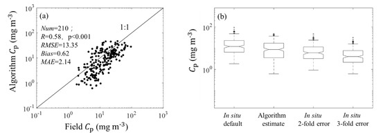
Figure 4.
(a) Comparison plot for the observed Cp and R17-derived Cp using the (676) dataset. (b) Box plots of the observed and derived corresponding to the default in situ values and in situ values with possibilities of 2- and 3-fold overestimations.
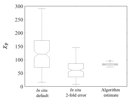
Figure 5.
Box plots of the observed corresponding to the default in situ values and in situ values with the possibility of 2-fold overestimation and algorithm-derived .
3.1.2. Validation of Estimations from (676)
Figure 6 shows the validation results for (676) estimations. The MAE and bias between (676)-estimated and field Cp were 1.9 and 1.39, respectively. The scatter points fell around the 1:1 line. The median value of the estimated Cp was similar to but slightly higher than that of the default field estimates (Figure 6b), which may result from the uncertainty of am and ChlaLH (see Section 4.1 for detailed discussion). The median value of the derived was 91.17, which was lower than the median value of field p (120.44) but higher than the median value of 2-fold-error field p (60.22) shown in Figure 5. Figure 7 shows the performances of R17 when using different input data. The values of R, RMSE, and MAE between (676)-derived and field Cp were similar to those between (676)-derived and field Cp. This result suggested that the performance of R17 applied to the (676) was similar to that of R17 applied to the . Accordingly, the (676) can be used to estimate the phytoplankton carbon in the SCS.
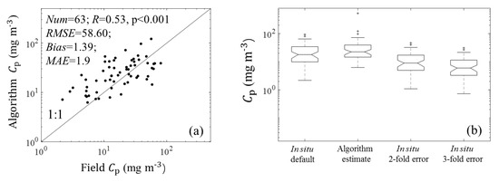
Figure 6.
(a) Comparison plot for the observed Cp and R17-derived Cp using the apg(). (b) Box plots of the observed and derived corresponding to the default in situ values and in situ values with possibilities of 2- and 3-fold overestimations.
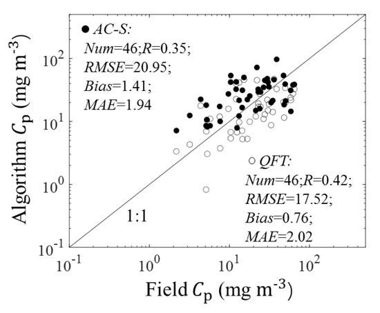
Figure 7.
Comparison plot for the observed Cp and R17-derived Cp. Note that the field Cp matched both (676)- and apg(λ)-derived Cp.
3.2. Vertical Variation of Phytoplankton Carbon and Related Bio-Parameters
3.2.1. Statistical Results from (676)
We analyzed the variations of total and size-partitioned phytoplankton carbon and related bio-parameters based on the results derived from (676) data within the euphotic layer covering the coastal region to the deep basin in the SCS. As shown in Table 2, the C varied from 2.38 to 62.02 mg m−3, with an average value of 16.53 mg m−3. The ranges of Cp, Cn, and Cm were 0.62–47.21, 0.21–25.70, and 0.0056–13.45 mg m−3, respectively. The average values of Cp, Cn, and Cm were 11.91, 3.69, and 0.93 mg m−3. Figure 8 shows the boxplot of Fp, Fn, and Fm. The median of Fp (0.67) was higher than the median of Fn (0.27), and the median of Fm (0.06) was lowest. Moreover, 87.44% of Fp were higher than the corresponding Fn and Fm. These results suggested that the picophytoplankton was the major contributor to C in the SCS, which is consistent with previous studies reporting that the open SCS is oligotrophic and that the picophytoplankton constitutes an essential component of the phytoplankton community [20,29,47]. The values of varied from 25.85 to 91.44, with an average value of 53.77. The value ranges of , , and were 72.15–96.36, 29.39–39.26, and 17.04–17.91, respectively. The value of C:POC is an important input in other phytoplankton carbon estimation models, and it is usually set to 30% [6,7]. However, the value of C:POC is not a constant, and it varies from 14% to 85% in different oceanic regions [13,48,49,50,51]. In our study, the C:POC value in the SCS ranged from 5.54% to 95.32%, and the average value was 41.27 ± 25.8% (Table 2). This variability of C:POC is consistent with the results reported in previous studies across a variety of oceanic regions [13,48,49,50,51].
Table 2.
Variations of C, size-partitioned phytoplankton carbon, POC, C:POC, , and the ratios of size-partitioned phytoplankton carbon to size-partitioned phytoplankton carbon based on the (676) dataset in the SCS.
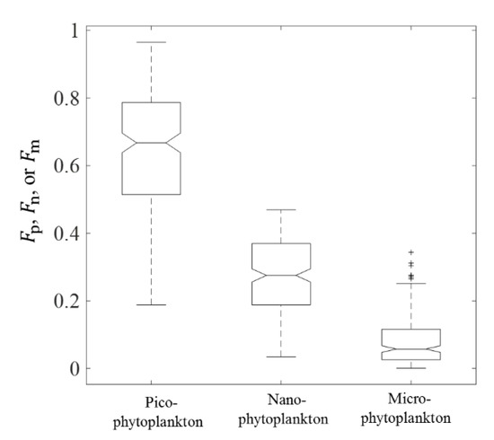
Figure 8.
Box plot of , , and values derived from R17 based on (676) data.
3.2.2. Vertical Profiles in the SCS Basin
To understand the basic vertical profile of total and size-partitioned phytoplankton carbon as well as χ in the open SCS, we plotted the results from the stations > 1000 m with strong stratification in the oligotrophic SCS basin. Figure 9 shows the values of C, size-partitioned phytoplankton carbon, and χ at four depths (0 or 5, 25, 50, and 75 m) derived from (676). Figure 10 shows the continuous high spatial resolution vertical profiles of these parameters derived from (676).
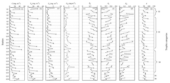
Figure 9.
Variabilities of (a) C, (b) Cp, (c) Cn, (d) Cm, (e) Fp, (f) Fn, (g) Fm, and (h) derived from (676) data at four depths (the filled circles from top to bottom represent values of the parameters at: 0 or 5, 25, 50, and 75 m in each bin, and the bins are divided by black dotted lines). The asterisks represent the Chla maximum among four depths at each station.
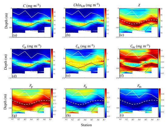
Figure 10.
The vertical profiles of (a) C, (b) ChlaLH, (c) , (d) Cp, (e) Cn, (f) Cm, (g) Fp, (h) Fn, and (i) Fm derived from (676) data in the open SCS (green stars in the Figure 1). White solid lines represent the MLD, and white dotted lines represent the depth of the C maximum, and black solid lines represent the ZT22, and black dotted lines represent the Zeu.
Vertical Profiles at Four Discrete Depths
According to the trophic categories, 92% of stations shown in Figure 9 were in the most oligotrophic environment (trophic categories were within S2–S4). The subsurface C maximums usually appeared at 50 or 75 m and were accompanied by the subsurface Chla maximums. The vertical profiles of Cp were similar to those of C at all stations. The values of Cp were the highest among Cp, Cn, and Cm at the depths of the subsurface C maximum. While 67% of vertical profiles of Cn were similar to those of C, 80% of vertical profiles of Cm were different from those of C, whereby the Cm maximums did not appear at the depths of the subsurface C maximum. Additionally, 88% of vertical profiles of Fp were similar to those of C. At the depth of the subsurface C maximum, the maximum values of Fp (generally > 0.5) were also observed at all stations. Most of vertical distributions of Fn and Fm showed the opposite trend as those of Fp, and the vertical maximum of Fp always coincided with the minimums of Fn and Fm and the highest value. This result indicated that at the depths of subsurface C maximum, the picophytoplankton was increasing, either in terms of total carbon biomass or fraction, which is consistent with the results reported in Uitz et al. [41] for S2–S4 waters and the results reported in Sauzède et al. [11] at the Bermuda Atlantic Times Series Study site from June to October. In most areas of the SCS basin, strong density stratification results in oligotrophic waters [52], thus the pico- and nanophytoplankton are dominant at the CML, and the contribution of Cm is low [41].
High Spatial Resolution Vertical Profile
Figure 10 shows seven higher spatial resolution vertical profiles of the phytoplankton carbon and bio-parameters, which were obtained from the (676) in the SCS basin. The stations with strong stratification, where water depths were >1000 m and measuring depths were >100 m, were chosen as the display stations. These vertical profiles derived from (676) show more detail about the variabilities of phytoplankton carbon and related bio-parameters within the whole euphotic zone. The (676)-derived vertical profiles of C, size-partitioned phytoplankton carbon, and related bio-parameters were similar to those derived from the (676) data. The CML was a universal feature at the seven stations, and the depths of the CML were all above the Zeu and ZT22. The subsurface C maximum (>20 mg m−3) appeared at 50–100 m with the subsurface Chla maximum layer and highest values. The values of Cp and Cn increased while the values of Cm decreased slightly at the CML. Figure 10g–i show that the Fp increased while Fn and Fm decreased at the CML. These results suggested that the contribution of picophytoplankton still increased while the contributions of nano- and microphytoplankton decreased at the CML.
4. Discussion
4.1. Sources of Uncertainty in the Algorithm
Two main sources of uncertainties in R17 are those associated with estimated values of and those in the allometric parameterization [13]. Deriving a new allometric relationship for phytoplankton in the SCS was out of the scope of our study, thus, we mainly focused on the uncertainties associated with . The value of was estimated based on the observed (676) or (676) [12]. If the value of is reliable, the uncertainty of the -estimated method in [12] is mainly due to the error in the value of am based on the field data. The value of am directly impacts the estimated values of from (676) or (676). To evaluate the overall uncertainties in the estimations of C and size-partitioned phytoplankton carbon, we added 0 to 30% uncertainties in the am into the algorithm. Regardless of whether (676) or (676) was used, the overestimation of am resulted in underestimation of C and Cp and overestimation of Cn and Cm (Figure 11). For the C derived from (676), when (676) was >0.025 m2 mg−1, a small underestimation (~5%) was observed, even when >20% uncertainty of am was added into the algorithm. However, significant underestimation (~30%) was observed when (676) was in the range of 0.020–0.025 m2 mg−1 and >20% uncertainty of am was added into the algorithm. For other cases, the uncertainty of algorithm-derived C showed an increasing trend with increasing uncertainty in am, but underestimation was generally <25%. For the Cp derived from the (676), when (676) was >0.025 m2 mg−1, a small underestimation (~5%) was observed even when >20% uncertainty of am was added into the algorithm. The underestimation increased up to 20–50% when (676) was <0.025 m2 mg−1 and >10% uncertainty of am was added into the algorithm. As for Cn and Cm, when (676) was in the range of 0.020–0.025 m2 mg−1, a significant overestimation (>100% for Cn and >1000% for Cm) was observed even when only 5% uncertainty of am was added into the algorithm. For other cases, smaller overestimation (~10% for Cn and ~30% for Cm) was observed. For (676), the uncertainty of algorithm-derived C and Cp showed an increasing trend with increasing uncertainty in am when (676) ranged from 0.011 to 0.013 m2 mg−1. Approximately 20% underestimation of C and 35% underestimation of Cp occurred when 10% uncertainty of am was added into the algorithm. For Cn and Cm, when (676) was >0.012 m2 mg−1, significant overestimations (>60% for Cn and >110% for Cm) were observed when >5% uncertainty of am was added into the algorithm.
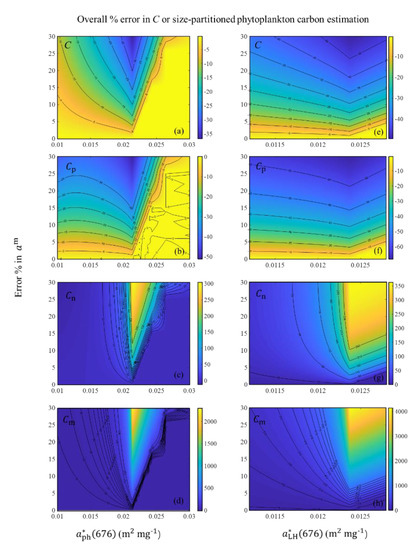
Figure 11.
Level of uncertainties in C and size-partitioned phytoplankton carbon computed by the R17 using the SCS field data. (a–d) Uncertainties in C, Cp, Cn, and Cm estimations due to possible errors in am for the uncertainty range 0–30% based on (676). (e–h) Uncertainties in C, Cp, Cn, and Cm estimations due to possible errors in am for the uncertainty range 0–30% based on (676).
On the whole, the effect of the uncertainty of am was relatively weak for underestimation of C [<35% for (676) data and <45% for (676)] and Cp [<40% for (676) data and <60% for (676)]. However, the effect of the uncertainty of am was significant for overestimation of Cn and Cm when (676) ranged from 0.02 to 0.025 m2 mg−1 or (676) was >0.012 m2 mg−1. Overall, the impact of uncertainty of am on the (676) data was greater than that on the (676) data. In this study, 80% of (676) values were in the range of 0.012–0.021 m2 mg−1, and 80% of (676) values were within 0.0116–0.0125 m2 mg−1, and different am values were chosen according to 95% quantile values for (676) and (676) data, respectively.
When the R17 algorithm was transplanted into the apg() data, ChlaLH, which was determined using the absorption line height method [45], also introduced uncertainties into the algorithm. Compared to the in situ Chla, the averaged relative error of ChlaLH could reach 20%. We evaluated the uncertainties in the estimations of C and size-partitioned phytoplankton carbon when 0–20% uncertainties were added into ChlaLH (Figure 12). The uncertainty of algorithm-derived C and size-partitioned phytoplankton carbon showed an increasing trend with increasing uncertainty in ChlaLH. A small uncertainty of C (around −20% to 10%) was observed when (676) was >0.0135 m2 mg−1 and even when 20% uncertainty was added into ChlaLH. For other cases, the uncertainty of C slightly increased but was <35% underestimation even if 20% uncertainty was added into the ChlaLH. Similarly, a small uncertainty of Cp (around −25% to 10%) was observed when (676) was >0.013 m2 mg−1 and 10% uncertainty was added into ChlaLH. The uncertainty of Cp (around −40% to −55%) increased when (676) was <0.0125 m2 mg−1 and >10% uncertainty was added into the ChlaLH. As for Cn and Cm, a small overestimation (<10%) was observed when (676) was >0.013 m2 mg−1 and 5% uncertainty was added into ChlaLH. When >10% uncertainty was added into ChlaLH, significant overestimation of Cn and Cm (>200% for Cn and >1000% for Cm) was observed when (676) ranged from 0.012 to 0.014 m2 mg−1.
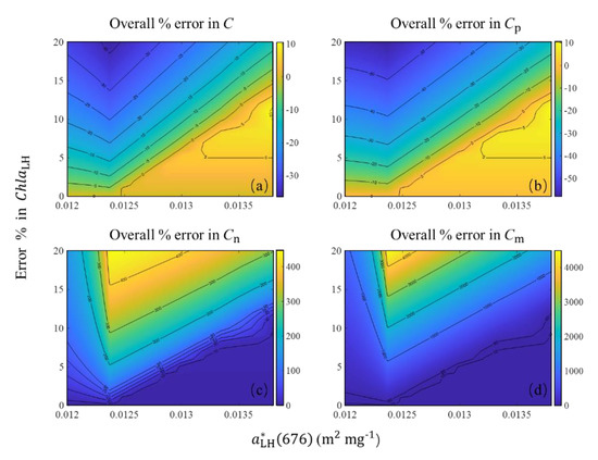
Figure 12.
Uncertainties in (a) C, (b) Cp, (c) Cn, and (d) Cm estimations due to possible errors in ChlaLH for the uncertainty range 0–20% based on (676) data.
Overall, the effect of ChlaLH uncertainty on C and Cp estimations (−35% to 10% for C and −55% to 10% for Cp when uncertainty of ChlaLH was <20%) was smaller than that on Cn and Cm estimations, which could reach >100% for Cn and >1000% for Cm when uncertainty of ChlaLH was >10%.
4.2. Relationship between C and Chla
The values of C and Chla are both used as proxies for the standing stock of phytoplankton biomass, and whether C or Chla is the appropriate proxy is controversial. The arguments for Chla are as follows: (i) chlorophyll-a is the transducer in the energy-ecosystem, and (ii) measurement of Chla is the simplest of all biological parameters [8]. For C, the argument is that C is a more direct parameter in the study of the carbon cycle and other climate-relevant variables in the ocean [8]. However, C and Chla can convert into each other through , and it is no longer necessary to make a choice between C and Chla [8]. Considering that the demand is for C in biogeochemical research but that Chla is the most commonly measured biological parameter, whether in situ or in remote sensing platform, we analyzed the relationship between C and Chla to facilitate the conversion between the two parameters. Because the value of varies among different algae species, we also analyzed the variability in relationships between C and Chla among different dominant phytoplankton species to provide more precise conversion parameters. As shown in Figure 13a, we detected significant covariation between C and Chla, which was consistent with the results reported in previous studies [8,53,54]. In previous studies, the form of C = iChlaj, where i and j are fitted parameters, was used to describe the relationship between C and Chla. The results from Buck et al. [54], Sathyendranath et al. [14], Marañón et al. [53], and Loisel et al. [55] are plotted in Figure 13a. The empirical relationships from Buck et al. [54] (C = 83Chla0.69) and Sathyendranath et al. [14] (C = 64Chla0.63) overestimated C when Chla was <0.3 mg m−3. The empirical relationships from Marañón et al. [53] (C = 62Chla0.89) and Loisel et al. [55] (C = 73Chla0.91) performed better for our data, although they also overestimated C when Chla was <0.2 mg m−3. The empirical relationship between C and Chla in our study was C = 46Chla0.8 (Table 3). The value of j could be used to describe how varied with Chla. The became constant when j = 1, which suggested that values of decreased as Chla increased when j was < 1, whereas the values of increased as Chla increased when j was > 1. All values of j in the five relationships were < 1. The value of j in our relationship was lower than those reported by Marañón et al. [53] and Loisel et al. [55] but higher than those reported by Buck et al. [54] and Sathyendranath et al. [14]. These results suggested that the values of decreased as Chla increased and that the variability in with Chla in our study was more significant than that found by Marañón et al. [53] and Loisel et al. [55] but more modest than that reported by Buck et al. [54] and Sathyendranath et al. [14].
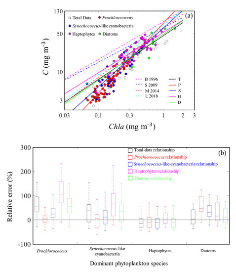
Figure 13.
(a) Relationship between C and Chla. The magenta, blue, red, and green dotted lines, respectively, represent the empirical relationships between C and Chla from Buck et al. (1996) [54] (curve B 1996), Sathyendranath et al. (2009) [14] (curve S 2009), Marañón et al. (2014) [53] (curve M 2014), and Loisel et al. (2018) [55] (curve L 2018). The black, red, blue, magenta, and green solid lines, respectively, represent the empirical relationships between C and Chla in our study for total data (curve T), Prochlorococcus (curve P), Synechococcus-like cyanobacteria (curve S), haptophytes (curve H), and diatom (curve D) dominated data. (b) Boxplots of relative errors of the total data, Prochlorococcus, Synechococcus-like cyanobacteria, haptophyte, and diatom Chla-to-C relationships in different sample groups dominated by different phytoplankton species. The black line represents relative error = 0.
Table 3.
Empirical power-law relationships between C and Chla in samples containing different dominant phytoplankton species in previous studies and this study.
In reality, changes in nutrients, irradiance, temperature, cell size (phytoplankton species) and Chla are all intimately related to each other in the marine environment, thus, it would be difficult to rule out the possible effects of these factors on [8]. As shown in Figure 13a, the dominant phytoplankton species varied from Prochlorococcus at the lowest Chla (~0.1 mg m−3) to diatoms at the highest Chla (~1 mg m−3). Xing et al. (2019) [21] reported that variability of phytoplankton community dominated the values of Chla:bbp at subsurface chlorophyll maximum layer in the SCS based on Bio-Argo data. Accordingly, in the SCS basin, change in dominant phytoplankton species may be one of the main factors resulting in variability in . To study the influence of variability in among different dominant algae species on Chla-to-C relationships, different empirical relationships between C and Chla were established among different dominant phytoplankton species based on our dataset (Table 3). Since dominant phytoplankton species will vary in the different specific range of Chla, the values of i in the relationships can be used to describe the rough values of different phytoplankton species. The values of i in Prochlorococcus (i = 78), Synechococcus-like cyanobacteria (i = 64), haptophytes (i = 53), and diatoms (i = 49) decreased sequentially, which suggested that the values of gradually decreased from Prochlorococcus to diatom dominant waters. The relative error between different relationship-estimated and -estimated C was calculated as 100%, where Crelationship was calculated using the empirical relationships in Table 3 for waters dominated by different phytoplankton species, and C was estimated based on . As shown in Figure 13b, the median relative error of the Prochlorococcus relationship (~4%) was around 0 when the dominant phytoplankton species was Prochlorococcus, whereas it increased to ~47% in diatom dominant waters. The median relative error of the Synechococcus-like cyanobacteria relationship was ~11% in Synechococcus-like cyanobacteria dominant waters, but the median relative errors of the Synechococcus-like cyanobacteria relationship had a greater deviation from 0% in Prochlorococcus (~24%), haptophyte (~–11%), and diatom (30%) dominant waters. For the haptophyte and diatom relationships, the largest median relative errors (both > 50%) were observed in Prochlorococcus dominant waters, and the median relative errors decreased as the cell size of the dominant algae increased. The smallest median relative errors of haptophytes (~4%) and diatoms (~9%) were observed in the haptophyte and diatom dominant waters, respectively. For the total relationship, the trend of median relative errors was similar to that of the diatoms relationship. The median relative errors of the total relationship decreased as the cell size of dominant algae increased. The largest median relative error of the total relationship was ~57% in the Prochlorococcus dominant waters, and in diatom dominant waters, the median relative error was ~3%. These results suggested that variability in values of due to changes in phytoplankton species can introduce apparent uncertainty to C converted from Chla when using a constant value of . Therefore, it is better to identify the dominant phytoplankton species to derive an accurate before converting Chla to C through .
4.3. General Vertical Profile of Phytoplankton Carbon in the SCS Basin
Figure 14a shows the general vertical distribution of C, size-partitioned phytoplankton carbon, and for oligotrophic stratified waters in the open SCS that is based on the profile shape shown in Figure 9 and Figure 10. It should be noted that Cn and Cm are sensitive to the choice of am, thus, interpretation of their profile shape should be made with caution. Overall, in the open SCS, the vertical profile of C displayed a Gaussian distribution with a peak near the bottom of the euphotic zone and the top of the nutricline, which was similar to that of the vertical Chla distribution [11,56]. C and Chla exhibited significant covariation (Figure 10 and Figure 13a), and it indicated that photoacclimation has little impact on the formation of the subsurface Chla maximum layer, which was consistent with results of Xing et al. [21].
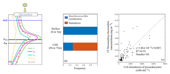
Figure 14.
(a) Schematic representation of the vertical profiles of C, Cp, Cn, Cm, and ; (b) the frequency of dominant phytoplankton species at the sea surface and the CML and (c) the relationship between the 19′hexanoyloxy-fucoxanthin concentrations and cell abundances of picoeukaryotes in the open stratified SCS.
The open SCS is an oligotrophic environment that is characterized by a “microbial loop” or “microbial food web” due to strong stratification [57]. Most (92%) of our survey stations were in the most oligotrophic condition. As shown in Figure 14a, the picophytoplankton dominated the phytoplankton biomass in the euphotic zone, and vertical distribution of Cp was similar to that of C (displayed a Gaussian distribution). This phenomenon was also reported by Uitz et al. [41], who found that the picophytoplankton biomass displayed a distinct deep maximum that was slightly sharper than that for nanophytoplankton biomass in S1–S4 trophic conditions. Meanwhile, the results in Sauzède et al. [11] at the Bermuda Atlantic Times Series Study site also showed that the picophytoplankton dominated the whole euphotic zone from June to October, and the deep maximum of picophytoplankton biomass was also sharper than that of nanophytoplankton biomass. We used HPLC data to analyze the dominant phytoplankton species and found that the phytoplankton community varied from Synechococcus-like cyanobacteria dominating at the sea surface to haptophytes dominating at the CML (Figure 14b). However, haptophytes are always classified as nanophytoplankton in many oceanic regions, ranging from tropical to polar systems [58,59], which was contrary to our result that the picophytoplankton was dominant at the CML. Moon-van der Staay et al. [59] reported that prymnesiophytes (class Prymnesiophyceae, division Haptophyta) was dominant among picoeukaryotes in the Pacific Ocean based on molecular biological techniques. Similarly, Ho et al. [60] suggested that haptophytes were the major picoeukaryotic phytoplankton in the northern SCS based on the relationship between concentrations of 19′hexanoyloxy-fucoxanthin and cell abundances of picoeukaryotes. Figure 14c shows a strong covariation between 19′hexanoyloxy-fucoxanthin concentrations and cell abundances of picoeukaryotes based on our data. A reasonable explanation for this contradictory result (haptophytes dominated the CML but picophytoplankton also dominated the CML) is that haptophytes in the open SCS were mostly pico-size. Therefore, the increase of haptophytes was the main factor involved in the formation of the CML. Thus, it was not surprising that the values of Fp and increased at the CML (Figure 9 and Figure 10) in the open stratified SCS.
5. Conclusions
We transplanted the remote sensing absorption-based phytoplankton carbon algorithm (R17) from Roy et al. [15] into field (676) and (676) to obtain vertical profiles of C and size-partitioned phytoplankton carbon in the SCS. The accuracy of am was an important factor affecting the accuracy of C and size-partitioned phytoplankton carbon estimations. Different values of am were chosen according to the 95% quantile values in the (676) and (676) datasets, respectively. For (676), the values of R, MAE, and bias between estimated and field Cp were 0.58, 2.14, and 0.62, respectively, and for apg(676) the values were 0.53, 1.9, and 1.39, respectively. The algorithm performed well for field data from the SCS. The vertical profiles of C and size-partitioned phytoplankton carbon in the SCS were then derived from field (676) and (676). The vertical profiles of C and Cp displayed Gaussian distributions, and the CML appeared at the bottom of the euphotic zone and the top of the nutricline in the stratified open SCS basin. Picophytoplankton was the dominant phytoplankton carbon contributor within the whole euphotic zone. The dominant picophytoplankton species varied from Synechococcus-like cyanobacteria at surface to pico-sized haptophytes at the CML. We detected strong covariation between C and Chla, and they can be converted to each other through an accurate value of . These results show the vertical profiles of phytoplankton biomass from the perspective of carbon mass and provide basic information for understanding primary production, the carbon cycle, and climate change in the SCS.
Author Contributions
Conceptualization: W.Z. (Wendi Zheng), W.Z. (Wen Zhou), and W.C.; methodology: W.Z. (Wendi Zheng) and W.Z. (Wen Zhou); software: W.Z. (Wendi Zheng); investigation: W.Z. (Wendi Zheng), L.D., K.Z., and Y.Z.; resources: W.Z. (Wen Zhou), and W.C.; original draft preparation: W.Z. (Wendi Zheng); review and editing: W.Z. (Wendi Zheng), W.Z. (Wen Zhou), W.C., G.W., and Y.L.; visualization: W.Z. (Wendi Zheng) and Y.L.; supervision: W.Z. (Wen Zhou) and W.C.; funding acquisition: W.C., W.Z. (Wen Zhou), and C.L. All authors have read and agreed to the published version of the manuscript.
Funding
This study was funded by the Key Special Project for Introduced Talents Team of Southern Marine Science and Engineering Guangdong Laboratory (Guangzhou) (GML2019ZD0602 and GML2019ZD0305); the National Natural Science Foundation of China (NSFC) (41976172,41976170, 41576030, 41976181, 41776044, and 41776045); the Science and Technology Planning Project of Guangzhou China (201707020023); State Key Laboratory of Tropical Oceanography, South China Sea Institute of Oceanology, Chinese Academy of Sciences (LTO, SCSIO, CAS) (LTOZZ2003).
Institutional Review Board Statement
Not applicable as this study did not involve human or animal subjects.
Informed Consent Statement
Not applicable as this study did not involve human or animal subjects.
Data Availability Statement
The data presented in this study are available on request from the corresponding authors.
Acknowledgments
We thank the National Natural Science Foundation of China and the South China Sea Institute of Oceanology of the Chinese Academy of Sciences for providing opportunities for the voyage surveys. We also thank all staff aboard the scientific research ships for helping with data collection and Jianlin Zhang for his help with measuring the picophytoplankton cell abundances in this study.
Conflicts of Interest
The authors declare no conflict of interest.
References
- Falkowski, P. Ocean Science: The power of plankton. Nat. Cell Biol. 2012, 483, S17–S20. [Google Scholar] [CrossRef]
- Field, C.B.; Behrenfeld, M.J.; Randerson, J.T.; Falkowski, P. Primary Production of the Biosphere: Integrating Terrestrial and Oceanic Components. Science 1998, 281, 237–240. [Google Scholar] [CrossRef]
- Barbieux, M.; Uitz, J.; Bricaud, A.; Organelli, E.; Poteau, A.; Schmechtig, C.; Gentili, B.; Obolensky, G.; Leymarie, E.; Penkerc’H, C.; et al. Assessing the Variability in the Relationship Between the Particulate Backscattering Coefficient and the Chlorophyll a Concentration From a Global Biogeochemical-Argo Database. J. Geophys. Res. Oceans 2018, 123, 1229–1250. [Google Scholar] [CrossRef]
- Siegel, D.; Behrenfeld, M.; Maritorena, S.; McClain, C.; Antoine, D.; Bailey, S.; Bontempi, P.; Boss, E.; Dierssen, H.; Doney, S.; et al. Regional to global assessments of phytoplankton dynamics from the SeaWiFS mission. Remote Sens. Environ. 2013, 135, 77–91. [Google Scholar] [CrossRef]
- Siegel, D.A.; Maritorena, S.; Nelson, N.B.; Behrenfeld, M.J. Independence and interdependencies among global ocean color properties: Reassessing the bio-optical assumption. J. Geophys. Res. Space Phys. 2005, 110, C07011. [Google Scholar] [CrossRef]
- Behrenfeld, M.J.; Boss, E.; Siegel, D.A.; Shea, D.M. Carbon-based ocean productivity and phytoplankton physiology from space. Glob. Biogeochem. Cycles 2005, 19, GB1006. [Google Scholar] [CrossRef]
- Kostadinov, T.S.; Milutinović, S.; Marinov, I.; Cabré, A. Carbon-based phytoplankton size classes retrieved via ocean color estimates of the particle size distribution. Ocean Sci. 2016, 12, 561–575. [Google Scholar] [CrossRef]
- Sathyendranath, S.; Platt, T.; Kovac, Z.; Dingle, J.; Jackson, T.; Brewin, R.J.W.; Franks, P.; Maranon, E.; Kulk, G.; Bouman, H.A. Reconciling models of primary production and photoacclimation. Appl. Opt. 2020, 59, C100–C114. [Google Scholar] [CrossRef] [PubMed]
- Graff, J.R.; Westberry, T.K.; Milligan, A.J.; Brown, M.B.; Dall’Olmo, G.; van Dongen-Vogels, V.; Reifel, K.M.; Behrenfeld, M.J. Analytical phytoplankton carbon measurements spanning diverse ecosystems. Deep. Sea Res. Part I Oceanogr. Res. Pap. 2015, 102, 16–25. [Google Scholar] [CrossRef]
- Brewin, R.J.; Sathyendranath, S.; Jackson, T.; Barlow, R.; Brotas, V.; Airs, R.L.; Lamont, T. Influence of light in the mixed-layer on the parameters of a three-component model of phytoplankton size class. Remote Sens. Environ. 2015, 168, 437–450. [Google Scholar] [CrossRef]
- Sauzède, R.; Claustre, H.; Jamet, C.; Uitz, J.; Ras, J.; Mignot, A.; D’Ortenzio, F. Retrieving the vertical distribution of chlorophyll a concentration and phytoplankton community composition from in situ fluorescence profiles: A method based on a neural network with potential for global-scale applications. J. Geophys. Res. Oceans 2015, 120, 451–470. [Google Scholar] [CrossRef]
- Roy, S.; Sathyendranath, S.; Bouman, H.; Platt, T. The global distribution of phytoplankton size spectrum and size classes from their light-absorption spectra derived from satellite data. Remote Sens. Environ. 2013, 139, 185–197. [Google Scholar] [CrossRef]
- Martínez-Vicente, V.; Evers-King, H.; Roy, S.; Kostadinov, T.S.; Tarran, G.A.; Graff, J.R.; Brewin, R.J.W.; Dall’Olmo, G.; Jackson, T.; Hickman, A.E.; et al. Intercomparison of Ocean Color Algorithms for Picophytoplankton Carbon in the Ocean. Front. Mar. Sci. 2017, 4, 378. [Google Scholar] [CrossRef]
- Sathyendranath, S.; Stuart, V.; Nair, A.; Oka, K.; Nakane, T.; Bouman, H.; Forget, M.-H.; Maass, H.; Platt, T. Carbon-to-chlorophyll ratio and growth rate of phytoplankton in the sea. Mar. Ecol. Prog. Ser. 2009, 383, 73–84. [Google Scholar] [CrossRef]
- Roy, S.; Sathyendranath, S.; Platt, T. Size-partitioned phytoplankton carbon and carbon-to-chlorophyll ratio from ocean colour by an absorption-based bio-optical algorithm. Remote Sens. Environ. 2017, 194, 177–189. [Google Scholar] [CrossRef]
- Westberry, T.; Behrenfeld, M.J.; Siegel, D.A.; Boss, E. Carbon-based primary productivity modeling with vertically resolved photoacclimation. Glob. Biogeochem. Cycles 2008, 22, GB2024. [Google Scholar] [CrossRef]
- Bellacicco, M.; Volpe, G.; Briggs, N.; Brando, V.; Pitarch, J.; Landolfi, A.; Colella, S.; Marullo, S.; Santoleri, R. Global Distribution of Non-algal Particles from Ocean Color Data and Implications for Phytoplankton Biomass Detection. Geophys. Res. Lett. 2018, 45, 7672–7682. [Google Scholar] [CrossRef]
- Bellacicco, M.; Cornec, M.; Organelli, E.; Brewin, R.J.W.; Neukermans, G.; Volpe, G.; Barbieux, M.; Poteau, A.; Schmechtig, C.; D’Ortenzio, F.; et al. Global Variability of Optical Backscattering by Non-algal particles from a Biogeochemical-Argo Data Set. Geophys. Res. Lett. 2019, 46, 9767–9776. [Google Scholar] [CrossRef]
- Kostadinov, T.S.; Siegel, D.A.; Maritorena, S. Retrieval of the particle size distribution from satellite ocean color observations. J. Geophys. Res. Space Phys. 2009, 114, C09015. [Google Scholar] [CrossRef]
- Chen, B.; Wang, L.; Song, S.; Huang, B.; Sun, J.; Liu, H. Comparisons of picophytoplankton abundance, size, and fluorescence between summer and winter in northern South China Sea. Cont. Shelf Res. 2011, 31, 1527–1540. [Google Scholar] [CrossRef]
- Xing, X.; Qiu, G.; Boss, E.; Wang, H. Temporal and Vertical Variations of Particulate and Dissolved Optical Properties in the South China Sea. J. Geophys. Res. Oceans 2019, 124, 3779–3795. [Google Scholar] [CrossRef]
- Wong, G.T.; Ku, T.-L.; Mulholland, M.; Tseng, C.-M.; Wang, D.-P. The SouthEast Asian Time-series Study (SEATS) and the biogeochemistry of the South China Sea—An overview. Deep. Sea Res. Part II Top. Stud. Oceanogr. 2007, 54, 1434–1447. [Google Scholar] [CrossRef]
- Wu, J.F.; Chung, L.S.; Wen, K.K.; Liu, Y.L.L.; Chen, H.Y.C.; Karl, D.M. Dissolved Inorganic Phosphorus, Dissolved Iron, and Trichodesmium in the Oligotrophic South China Sea. Global. Biogeochemical. Cycles. 2003, 17, 1008. [Google Scholar] [CrossRef]
- Zhang, W.-Z.; Wang, H.; Chai, F.; Qiu, G. Physical drivers of chlorophyll variability in the open South China Sea. J. Geophys. Res. Oceans 2016, 121, 7123–7140. [Google Scholar] [CrossRef]
- Wang, L.; Koblinsky, C.; Howden, S.; Huang, N. Interannual variability in the South China Sea from expendable bathythermograph data. J. Geophys. Res. Space Phys. 1999, 104, 23509–23523. [Google Scholar] [CrossRef]
- Xue, H.; Chai, F.; Pettigrew, N.; Xu, D.; Shi, M.; Xu, J. Kuroshio intrusion and the circulation in the South China Sea. J. Geophys. Res. Space Phys. 2004, 109. [Google Scholar] [CrossRef]
- Gong, X.; Shi, J.; Gao, H. Modeling seasonal variations of subsurface chlorophyll maximum in South China Sea. J. Ocean. Univ. China 2014, 13, 561–571. [Google Scholar] [CrossRef]
- Lu, Z.; Gan, J.; Dai, M.; Cheung, A.Y. The influence of coastal upwelling and a river plume on the subsurface chlorophyll maximum over the shelf of the northeastern South China Sea. J. Mar. Syst. 2010, 82, 35–46. [Google Scholar] [CrossRef]
- Ning, X.; Chai, F.; Xue, H.; Cai, Y.; Liu, C.; Shi, J. Physical-biological oceanographic coupling influencing phytoplankton and primary production in the South China Sea. J. Geophys. Res. Space Phys. 2004, 109, C10005. [Google Scholar] [CrossRef]
- Wang, G.; Cao, W.; Yang, D.; Zhao, J. Partitioning particulate absorption coefficient into contributions of phytoplankton and nonalgal particles: A case study in the northern South China Sea. Estuar. Coast. Shelf Sci. 2008, 78, 513–520. [Google Scholar] [CrossRef]
- Stramski, D.; Reynolds, R.A.; Kaczmarek, S.; Uitz, J.; Zheng, G. Correction of pathlength amplification in the filter-pad technique for measurements of particulate absorption coefficient in the visible spectral region. Appl. Opt. 2015, 54, 6763–6782. [Google Scholar] [CrossRef]
- Sullivan, J.M.; Twardowski, M.S.; Zaneveld, J.R.V.; Moore, C.M.; Barnard, A.H.; Donaghay, P.L.; Rhoades, B. Hyperspectral temperature and salt dependencies of absorption by water and heavy water in the 400–750 nm spectral range. Appl. Opt. 2006, 45, 5294–5309. [Google Scholar] [CrossRef] [PubMed]
- Zaneveld, R.V.; Kitchen, J.C.; Moore, C. The Scattering Error-Correction of Reflecting-Tube Absorption Meters. Ocean Opt. 1994, Xii, 44–55. [Google Scholar]
- Hamilton, E. A manual of chemical & biological methods for seawater analysis. Mar. Pollut. Bull. 1984, 15, 419–420. [Google Scholar] [CrossRef]
- Knap, A.; Michaels, A.; Close, A. Protocols for the Joint Global Ocean Flux Study (Jgofs) Core Measurements; UNESCO: Paris, France, 1996. [Google Scholar]
- Vidussi, F.; Claustre, H.; Bustillos Guzman, J.; Cailliau, C.; Marty, J.C. Determination of Chlorophylls and Carotenoids of Marine Phytoplankton: Separation of Chlorophyll a from Divinyl-Chlorophyll a and Zeaxanthin from Lutein. J. Plankton Res. 1996, 18, 2377–2382. [Google Scholar] [CrossRef]
- Alvain, S.; Moulin, C.; Dandonneau, Y.; Bréon, F.-M. Remote sensing of phytoplankton groups in case 1 waters from global SeaWiFS imagery. Deep. Sea Res. Part I Oceanogr. Res. Pap. 2005, 52, 1989–2004. [Google Scholar] [CrossRef]
- Marie, D.; Partensky, F.; Vaulot, D.; Brussaard, C. Enumeration of Phytoplankton, Bacteria, and Viruses in Marine Samples. Curr. Protoc. Cytom. 1999, 10, 1–15. [Google Scholar] [CrossRef]
- Wang, G.; Zhou, W.; Cao, W.; Yin, J.; Yang, Y.; Sun, Z.; Zhang, Y.; Zhao, J. Variation of particulate organic carbon and its relationship with bio-optical properties during a phytoplankton bloom in the Pearl River estuary. Mar. Pollut. Bull. 2011, 62, 1939–1947. [Google Scholar] [CrossRef]
- Cao, W.; Yang, Y. A Bio-optical model for ocean photosynthetic available radiation. J. Trop. Oceanogr. 2002, 21, 47–54. (In Chinese) [Google Scholar]
- Uitz, J.; Claustre, H.; Morel, A.; Hooker, S.B. Vertical distribution of phytoplankton communities in open ocean: An assessment based on surface chlorophyll. J. Geophys. Res. Space Phys. 2006, 111, C08005. [Google Scholar] [CrossRef]
- Seegers, B.N.; Stumpf, R.P.; Schaeffer, B.A.; Loftin, K.A.; Werdell, P.J. Performance metrics for the assessment of satellite data products: An ocean color case study. Opt. Express 2018, 26, 7404–7422. [Google Scholar] [CrossRef]
- Roy, S.; Sathyendranath, S.; Platt, T. Retrieval of phytoplankton size from bio-optical measurements: Theory and applications. J. R. Soc. Interface 2010, 8, 650–660. [Google Scholar] [CrossRef] [PubMed]
- Menden-Deuer, S.; Lessard, E.J. Carbon to volume relationships for dinoflagellates, diatoms, and other protist plankton. Limnol. Oceanogr. 2000, 45, 569–579. [Google Scholar] [CrossRef]
- Roesler, C.S.; Barnard, A.H. Optical proxy for phytoplankton biomass in the absence of photophysiology: Rethinking the absorption line height. Methods Oceanogr. 2013, 7, 79–94. [Google Scholar] [CrossRef]
- Buitenhuis, E.T.; Li, W.K.W.; Vaulot, D.; Lomas, M.W.; Landry, M.R.; Partensky, F.; Karl, D.M.; Ulloa, O.; Campbell, L.; Jacquet, S.; et al. Picophytoplankton biomass distribution in the global ocean. Earth Syst. Sci. Data 2012, 4, 37–46. [Google Scholar] [CrossRef]
- Liu, H.; Chang, J.; Tseng, C.-M.; Wen, L.-S.; Liu, K.-K. Seasonal variability of picoplankton in the Northern South China Sea at the SEATS station. Deep. Sea Res. Part II Top. Stud. Oceanogr. 2007, 54, 1602–1616. [Google Scholar] [CrossRef]
- Eppley, R.W.; Chavez, F.P.; Barber, R.T. Standing Stocks of Particulate Carbon and Nitrogen in the Equatorial Pacific at 150-Degrees-W. J. Geophys. Res. Ocean. 1992, 97, 655–661. [Google Scholar] [CrossRef]
- Gundersen, K.; Orcutt, K.M.; Purdie, D.A.; Michaels, A.F.; Knap, A.H. Particulate organic carbon mass distribution at the Bermuda Atlantic Time-series Study (BATS) site. Deep. Sea Res. Part II Top. Stud. Oceanogr. 2001, 48, 1697–1718. [Google Scholar] [CrossRef]
- DuRand, M.D.; Olson, R.J.; Chisholm, S.W. Phytoplankton population dynamics at the Bermuda Atlantic Time-series station in the Sargasso Sea. Deep. Sea Res. II Top. Stud. Oceanogr. 2001, 48, 1983–2003. [Google Scholar] [CrossRef]
- Oubelkheir, K.; Claustre, H.; Sciandra, A.; Babin, M. Bio-optical and biogeochemical properties of different trophic regimes in oceanic waters. Limnol. Oceanogr. 2005, 50, 1795–1809. [Google Scholar] [CrossRef]
- Liang, W.; Tang, D.; Luo, X. Phytoplankton size structure in the western South China Sea under the influence of a ‘jet-eddy system’. J. Mar. Syst. 2018, 187, 82–95. [Google Scholar] [CrossRef]
- Marañón, E.; Cermeño, P.; Huete-Ortega, M.; López-Sandoval, D.C.; Mouriño-Carballido, B.; Rodríguez-Ramos, T. Resource Supply Overrides Temperature as a Controlling Factor of Marine Phytoplankton Growth. PLoS ONE 2014, 9, e99312. [Google Scholar] [CrossRef]
- Buck, K.; Chavezt, F.; Campbell, L. Basin-wide distributions of living carbon components and the inverted trophic pyramid of the central gyre of the North Atlantic Ocean, summer 1993. Aquat. Microb. Ecol. 1996, 10, 283–298. [Google Scholar] [CrossRef]
- Loisel, L.D.H.; Dessailly, S.; Sathyendranath, H.E.; Vantrepotte, S.; Thomalla, A.M.; D’andon, O.H.F. A Satellite View of the Particulate Organic Carbon and Its Algal and Non-Algal Carbon Pools. In Proceedings of the Ocean Optics XXIV, Dubrovnik, Croatia, 7–12 October 2018. [Google Scholar]
- Gong, X.; Shi, J.; Gao, H.W.; Yao, X.H. Steady-state solutions for subsurface chlorophyll maximum in stratified water columns with a bell-shaped vertical profile of chlorophyll. Biogeosciences 2015, 12, 905–919. [Google Scholar] [CrossRef]
- Wang, L.; Huang, B.; Chiang, K.-P.; Liu, X.; Chen, B.; Xie, Y.; Xu, Y.; Hu, J.; Dai, M. Physical-Biological Coupling in the Western South China Sea: The Response of Phytoplankton Community to a Mesoscale Cyclonic Eddy. PLoS ONE 2016, 11, e0153735. [Google Scholar] [CrossRef]
- Andersen, R.A.; Bidigare, R.R.; Keller, M.D.; Latasa, M. A comparison of HPLC pigment signatures and electron microscopic observations for oligotrophic waters of the North Atlantic and Pacific Oceans. Deep. Sea Res. II Top. Stud. Oceanogr. 1996, 43, 517–537. [Google Scholar] [CrossRef]
- Moon-van der Staay, S.Y.; van der Staay, G.W.M.; Guillou, L.; Vaulot, D.; Claustre, H.; Medlin, L.K. Abundance and Diversity of Prymnesiophytes in the Picoplankton Community from the Equatorial Pacific Ocean Inferred from 18s Rdna Sequences. Limnol. Oceanogr. 2000, 45, 98–109. [Google Scholar] [CrossRef]
- Ho, T.-Y.; Pan, X.; Yang, H.-H.; George, T.W.; Shiah, F.-K. Controls on temporal and spatial variations of phytoplankton pigment distribution in the Northern South China Sea. Deep. Sea Res. II Top. Stud. Oceanogr. 2015, 117, 65–85. [Google Scholar] [CrossRef]


Publisher’s Note: MDPI stays neutral with regard to jurisdictional claims in published maps and institutional affiliations. |
© 2021 by the authors. Licensee MDPI, Basel, Switzerland. This article is an open access article distributed under the terms and conditions of the Creative Commons Attribution (CC BY) license (http://creativecommons.org/licenses/by/4.0/).