
Sampling-Based Path Planning for High-Quality Aerial 3D Reconstruction of Urban Scenes


Abstract
1. Introduction
- We devise a simple, yet effective viewpoint generation method, which significantly reduces the search space by the association with the surface clusters of the 3D prior of the scene estimated by an initial flight pass.
- We propose a novel viewpoint selection method that combines candidate viewpoints with sample points to fully cover the entire scene, especially for undersampled areas in the initial flight pass, which gives rise to a highly complete 3D reconstruction with as few acquired images as possible.
2. Related Work
2.1. Aerial Reconstruction
2.2. Path Planning for Scene Reconstruction
3. Proposed Method
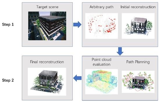
3.1. Overview
3.2. Prior Model Construction
3.2.1. Coarse Reconstruction
3.2.2. Pre-Processing
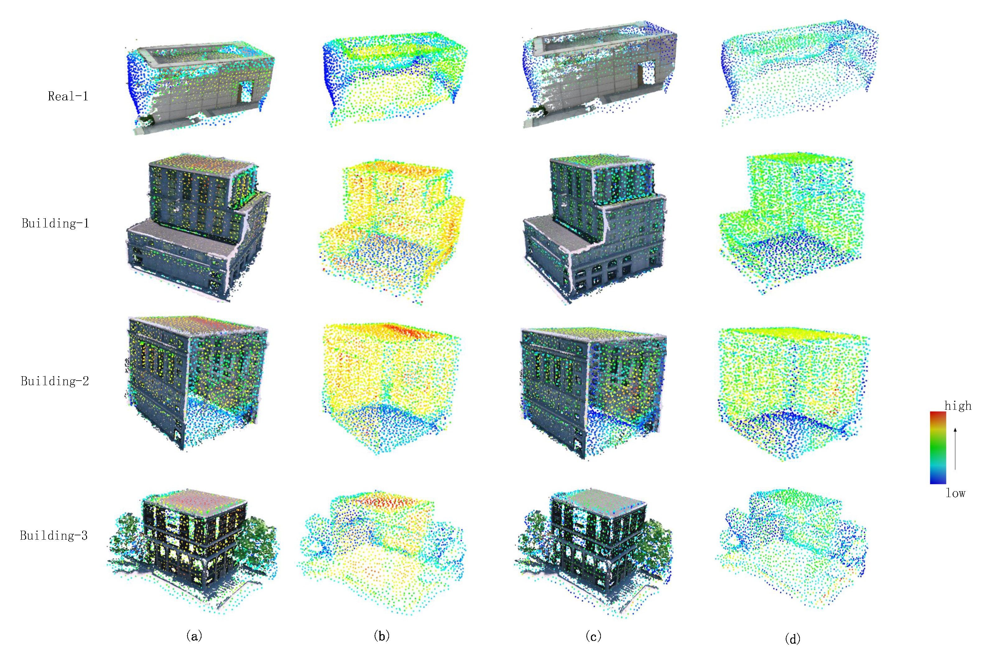
3.2.3. Quality Evaluation of the Initial Point Cloud
3.3. Aerial Viewpoint Generation
3.3.1. View Sampling Space
3.3.2. Viewpoint Selection
3.4. Path Planning
4. Results
4.1. Experimental Setting
4.1.1. Data Set
4.1.2. Reconstruction
4.1.3. Evaluation Metrics
4.1.4. Sample Scale
4.2. Method Analysis
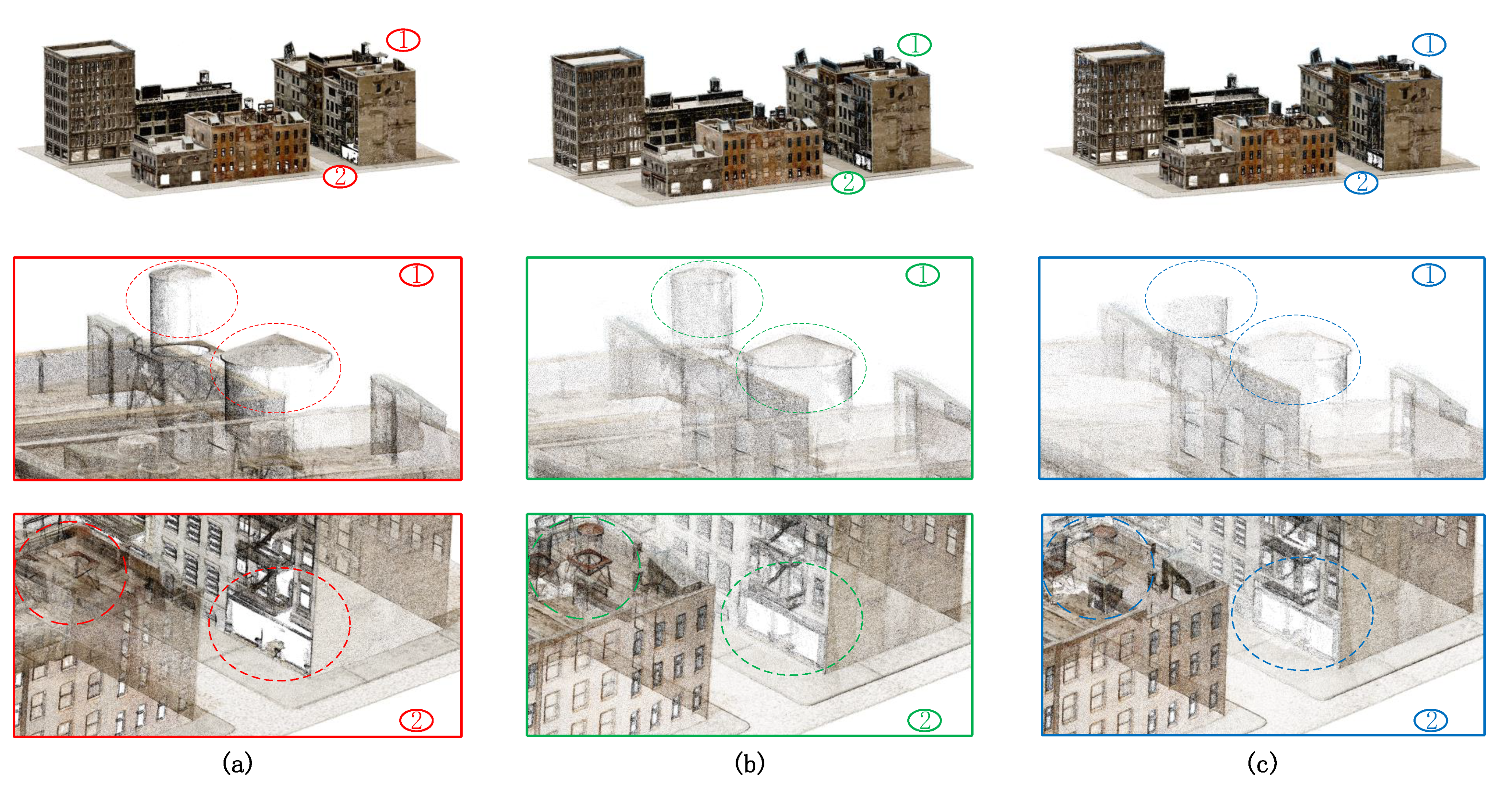
4.3. Comparison with a State-of-the-Art Approach
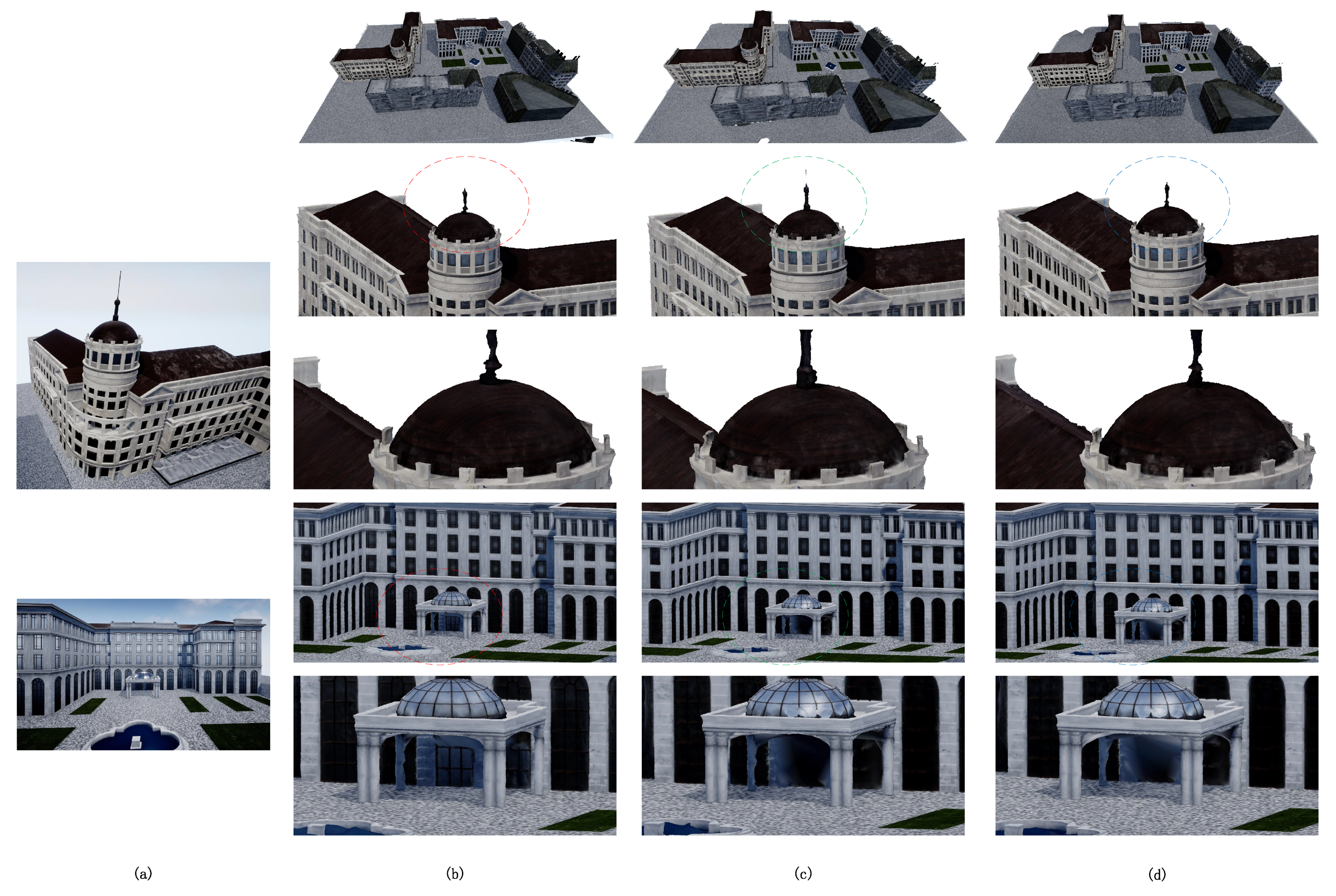
4.4. Comparison with the Pre-Defined Flight Paths
5. Conclusions
Author Contributions
Funding
Conflicts of Interest
References
- Boonpook, W.; Tan, Y.; Liu, H.; Zhao, B.; He, L. UAV-BASED 3D Urban Environment Monitoring. ISPRS Ann. Photogramm. Remote Sens. Spat. Inf. Sci. 2018, 37–43. [Google Scholar] [CrossRef]
- Barmpounakis, E.N.; Vlahogianni, E.I.; Golias, J.C. Unmanned Aerial Aircraft Systems for transportation engineering: Current practice and future challenges. Int. J. Transp. Sci. Technol. 2016, 5, 111–122. [Google Scholar] [CrossRef]
- Zhang, C.; Kovacs, J.M. The application of small unmanned aerial systems for precision agriculture: A review. Precis. Agric. 2012, 13, 693–712. [Google Scholar] [CrossRef]
- Nikolic, J.; Burri, M.; Rehder, J.; Leutenegger, S.; Huerzeler, C.; Siegwart, R. A UAV system for inspection of industrial facilities. In Proceedings of the 2013 IEEE Aerospace Conference, Big Sky, MT, USA, 2–9 March 2013; pp. 1–8. [Google Scholar]
- Majdik, A.; Till, C.; Scaramuzza, D. The Zurich urban micro aerial vehicle dataset. Int. J. Robot. Res. 2017, 36, 269–273. [Google Scholar] [CrossRef]
- Vu, H.; Labatut, P.; Pons, J.; Keriven, R. High Accuracy and Visibility-Consistent Dense Multiview Stereo. IEEE Trans. Pattern Anal. Mach. Intell. 2012, 34, 889–901. [Google Scholar] [CrossRef] [PubMed]
- Garcia-Dorado, I.; Demir, I.; Aliaga, D.G. Automatic urban modeling using volumetric reconstruction with surface graph cuts. Comput. Graph. 2013, 37, 896–910. [Google Scholar] [CrossRef]
- Li, M.; Nan, L.; Smith, N.; Wonka, P. Reconstructing building mass models from UAV images. Comput. Graph. 2016, 54, 84–93. [Google Scholar] [CrossRef]
- Wu, M.; Popescu, V. Efficient VR and AR Navigation Through Multiperspective Occlusion Management. IEEE Trans. Vis. Comput. Graph. 2018, 24, 3069–3080. [Google Scholar] [CrossRef] [PubMed]
- Seitz, S.M.; Curless, B.; Diebel, J.; Scharstein, D.; Szeliski, R. A Comparison and Evaluation of Multi-View Stereo Reconstruction Algorithms. In Proceedings of the 2016 IEEE Computer Society Conference on Computer Vision and Pattern Recognition, New York, NY, USA, 17–22 June 2006; Volume 1, pp. 519–528. [Google Scholar]
- Mancini, F.; Dubbini, M.; Gattelli, M.; Stecchi, F.; Fabbri, S.; Gabbianelli, G. Using Unmanned Aerial Vehicles (UAV) for High-Resolution Reconstruction of Topography: The Structure from Motion Approach on Coastal Environments. Remote Sens. 2013, 5, 6880–6898. [Google Scholar] [CrossRef]
- Schönberger, J.L.; Zheng, E.; Frahm, J.M.; Pollefeys, M. Pixelwise View Selection for Unstructured Multi-View Stereo. In Computer Vision—ECCV 2016; Leibe, B., Matas, J., Sebe, N., Welling, M., Eds.; Springer International Publishing: Cham, Switzerland, 2016; pp. 501–518. [Google Scholar]
- Schönberger, J.L.; Zheng, E.; Pollefeys, M.; Frahm, J.M. Pixelwise View Selection for Unstructured Multi-View Stereo. In Proceedings of the European Conference on Computer Vision (ECCV), Amsterdam, The Netherlands, 11–14 October 2016. [Google Scholar]
- Roberts, M.; Shah, S.; Dey, D.; Truong, A.; Sinha, S.N.; Kapoor, A.; Hanrahan, P.; Joshi, N. Submodular Trajectory Optimization for Aerial 3D Scanning. In Proceedings of the IEEE International Conference on Computer Vision, Venice, Italy, 22–29 October 2017; pp. 5334–5343. [Google Scholar]
- Hepp, B.; Nießner, M.; Hilliges, O. Plan3D: Viewpoint and Trajectory Optimization for Aerial Multi-View Stereo Reconstruction. ACM Trans. Graph. 2018, 38, 1–7. [Google Scholar] [CrossRef]
- Schönberger, J.L.; Frahm, J.M. Structure-from-Motion Revisited. In Proceedings of the 2016 IEEE Conference on Computer Vision and Pattern Recognition (CVPR), Las Vegas, NV, USA, 27–30 June 2016. [Google Scholar]
- Xu, K.; Huang, H.; Shi, Y.; Li, H.; Long, P.; Caichen, J.; Sun, W.; Chen, B. Autoscanning for Coupled Scene Reconstruction and Proactive Object Analysis. Acm Trans. Graph. 2015, 34, 177:1–177:14. [Google Scholar] [CrossRef]
- Wu, S.; Sun, W.; Long, P.; Huang, H.; Cohen-Or, D.; Gong, M.; Deussen, O.; Chen, B. Quality-Driven Poisson-Guided Autoscanning. ACM Trans. Graph. 2014, 33. [Google Scholar] [CrossRef]
- Fernández-Hernandez, J.; González-Aguilera, D.; Rodríguez-Gonzálvez, P.; Mancera-Taboada, J. Image-Based Modelling from Unmanned Aerial Vehicle (UAV) Photogrammetry: An Effective, Low-Cost Tool for Archaeological Applications. Archaeometry 2015, 57, 128–145. [Google Scholar] [CrossRef]
- Mohammed, F.; Idries, A.; Mohamed, N.; Al-Jaroodi, J.; Jawhar, I. UAVs for smart cities: Opportunities and challenges. In Proceedings of the 2014 International Conference on Unmanned Aircraft Systems (ICUAS), Orlando, FL, USA, 27–30 May 2014; pp. 267–273. [Google Scholar]
- Hartley, R.I.; Zisserman, A. Multiple View Geometry in Computer Vision, 2nd ed.; Cambridge University Press: Cambridge, UK, 2004; ISBN 0521540518. [Google Scholar]
- Cadena, C.; Carlone, L.; Carrillo, H.; Latif, Y.; Scaramuzza, D.; Neira, J.; Reid, I.; Leonard, J.J. Past, Present, and Future of Simultaneous Localization and Mapping: Toward the Robust-Perception Age. IEEE Trans. Robot. 2016, 32, 1309–1332. [Google Scholar] [CrossRef]
- Suzuki, T.; Amano, Y.; Hashizume, T.; Shinji, S. 3D Terrain Reconstruction by Small Unmanned Aerial Vehicle Using SIFT-Based Monocular SLAM. J. Robot. Mechatron. 2011, 23, 292–301. [Google Scholar] [CrossRef]
- Teixeira, L.; Chli, M. Real-time local 3D reconstruction for aerial inspection using superpixel expansion. In Proceedings of the 2017 IEEE International Conference on Robotics and Automation (ICRA), Singapore, 29 May–3 June 2017; pp. 4560–4567. [Google Scholar] [CrossRef]
- Kriegel, S.; Rink, C.; Bodenmüller, T.; Narr, A.; Hirzinger, G. Next-Best-Scan Planning for Autonomous 3D Modeling. In Proceedings of the 2012 IEEE/RSJ International Conference on Intelligent Robots and Systems, Vilamoura-Algarve, Portugal, 7–12 October 2012. [Google Scholar]
- Newcombe, R.A.; Izadi, S.; Hilliges, O.; Molyneaux, D.; Kim, D.; Davison, A.J.; Kohi, P.; Shotton, J.; Hodges, S.; Fitzgibbon, A. KinectFusion: Real-time dense surface mapping and tracking. In Proceedings of the 2011 10th IEEE International Symposium on Mixed and Augmented Reality, Basel, Switzerland, 26–29 October 2011; pp. 127–136. [Google Scholar]
- Peng, C.; Isler, V. Adaptive View Planning for Aerial 3D Reconstruction. In Proceedings of the 2019 International Conference on Robotics and Automation (ICRA), Montreal, QC, Canada, 20–24 May 2019; pp. 2981–2987. [Google Scholar]
- Smith, N.; Moehrle, N.; Goesele, M.; Heidrich, W. Aerial Path Planning for Urban Scene Reconstruction: A Continuous Optimization Method and Benchmark. ACM Trans. Graph. 2018, 37. [Google Scholar] [CrossRef]
- Qu, Y.; Huang, J.; Zhang, X. Rapid 3D Reconstruction for Image Sequence Acquired from UAV Camera. Sensors 2018, 18, 225. [Google Scholar]
- Rublee, E.; Rabaud, V.; Konolige, K.; Bradski, G. ORB: An efficient alternative to SIFT or SURF. In Proceedings of the 2011 International Conference on Computer Vision, Barcelona, Spain, 6–13 November 2011; pp. 2564–2571. [Google Scholar]
- Mur-Artal, R.; Tardós, J.D. ORB-SLAM2: An Open-Source SLAM System for Monocular, Stereo, and RGB-D Cameras. IEEE Trans. Robot. 2017, 33, 1255–1262. [Google Scholar] [CrossRef]
- Corsini, M.; Cignoni, P.; Scopigno, R. Efficient and Flexible Sampling with Blue Noise Properties of Triangular Meshes. IEEE Trans. Vis. Comput. Graph. 2012, 18, 914–924. [Google Scholar] [CrossRef]
- Kazhdan, M.; Bolitho, M.; Hoppe, H. Poisson Surface Reconstruction. In Proceedings of the Fourth Eurographics Symposium on Geometry Processing (SGP ’06), Cagliari, Italy, 26–28 June 2006; Eurographics Association: Goslar, Germany, 2006; pp. 61–70. [Google Scholar]
- Dorigo, M.; Gambardella, L.M. Ant colonies for the travelling salesman problem—ScienceDirect. Biosystems 1997, 43, 73–81. [Google Scholar] [CrossRef]
- Stützle, T.; Dorigo, M. ACO Algorithms for the Traveling Salesman Problem. Evol. Algorithms Eng. Comput. Sci. 1999, 4, 163–183. [Google Scholar]


| Scene | #Voxels | w/o Local Viewpoints | w. Local Viewpoints | ||||||
|---|---|---|---|---|---|---|---|---|---|
| #Local | #Global | Time (s) | Completeness (%) | #Local | #Global | Time (s) | Completeness (%) | ||
| Building-1 | 42,452 | 0 | 108 | 109.419 | 56.987 | 120 | 90 | 108.902 | 74.079 |
| Building-2 | 51,452 | 0 | 104 | 92.355 | 51.759 | 116 | 89 | 95.596 | 71.367 |
| Building-3 | 23,060 | 0 | 53 | 26.74 | 43.612 | 114 | 39 | 26.771 | 65.954 |
| #Viewpoints | Methods | Time (s) | Length (m) |
|---|---|---|---|
| 7 | BnB | 0.316 | 43.286 |
| ACO | 0.724 | 43.286 | |
| 8 | BnB | 1.362 | 52.334 |
| ACO | 0.827 | 52.334 | |
| 9 | BnB | 4.647 | 54.588 |
| ACO | 0.999 | 54.588 | |
| 10 | BnB | 18.75 | 57.7 |
| ACO | 1.206 | 57.7 | |
| 11 | BnB | 59.213 | 57.948 |
| ACO | 1.402 | 57.948 | |
| 12 | BnB | 463.364 | 60.366 |
| ACO | 1.551 | 60.366 |
| #Viewpoints | Methods | Time (s) | Length (m) |
|---|---|---|---|
| 50 | PSO | 15.031 | 230.999 |
| ACO | 36.337 | 227.461 | |
| 100 | PSO | 25.52 | 566.299 |
| ACO | 129.613 | 566.912 | |
| 150 | PSO | 42.488 | 979.863 |
| ACO | 310.765 | 925.306 | |
| 200 | PSO | 54.199 | 1329.885 |
| ACO | 519.66 | 1280.699 | |
| 300 | PSO | 94.681 | 2127.964 |
| ACO | 1208.345 | 1966.103 | |
| 433 | PSO | 148.526 | 3012.832 |
| ACO | 2396.544 | 2812.758 |
| Scenes | Methods | #Images | Path Length (m) | Error 90% (m) | Error 95% (m) | Completeness 0.075 m (%) |
|---|---|---|---|---|---|---|
| NY-1 | Grid | 484 | 2618.3 | 0.076 | 1.618 | 28.46 |
| Smith et al. | 433 | 2807.7 | 0.038 | 0.057 | 46.47 | |
| Ours (low) | 204 | 2091.4 | 0.069 | 1.021 | 38.43 | |
| Ours (high) | 247 | 2544.9 | 0.031 | 0.048 | 47.89 | |
| GOTH-1 | Grid | 576 | 4192.9 | 0.083 | 0.206 | 20.39 |
| Smith et al. | 588 | 4213.2 | 0.029 | 0.048 | 53.36 | |
| Ours (low) | 192 | 2565.3 | 0.036 | 0.066 | 40.82 | |
| Ours (high) | 291 | 3153.1 | 0.026 | 0.047 | 54.82 | |
| UK-1 | Grid | 961 | 6774 | 0.7126 | 1.596 | 5.44 |
| Smith et al. | 923 | 7819.3 | 0.112 | 0.146 | 32.29 | |
| Ours (low) | 203 | 2989.6 | 0.134 | 0.152 | 27.81 | |
| Ours (high) | 362 | 4600.3 | 0.103 | 0.147 | 31.81 |
| Scenes | Pre-Processing (s) | Quality Estimation (s) | Viewpoint Generation (s) | Path Planning (s) | Total (s) | ||
|---|---|---|---|---|---|---|---|
| Completeness | Smoothness | Local | Global | ||||
| NY-1 | 5.293 | 0.294 | 0.459 | 2.992 | 23.294 | 15.933 | 48.265 |
| GOTH-1 | 9.042 | 0.316 | 0.818 | 3.118 | 23.874 | 17.188 | 54.356 |
| UK-1 | 15.068 | 0.311 | 1.309 | 2.634 | 17.83 | 15.338 | 52.49 |
| Scenes | Methods | Pitch () | Roll () | Yaw () |
|---|---|---|---|---|
| NY-1 | Smith et al. | 12.551 | 0 | 49.687 |
| Ours (low) | 8.536 | 0 | 23.905 | |
| Ours (high) | 9.023 | 0 | 24.658 | |
| GOTH-1 | Smith et al. | 17.431 | 0 | 76.474 |
| Ours (low) | 12.709 | 0 | 36.487 | |
| Ours (high) | 15.126 | 0 | 59.74 | |
| UK-1 | Smith et al. | 13.77 | 0 | 75.922 |
| Ours (low) | 14.184 | 0 | 33.172 | |
| Ours (high) | 12.438 | 0 | 31.472 |
| Scenes | Path Models | #Images | #Points | > 0.5 Pct. | #Voxels | Points > 10 Pct. | Points > 5 Pct. | Points > 3 Pct. |
|---|---|---|---|---|---|---|---|---|
| Real-1 | circular | 180 | 485,112 | 22.39% | 264,600 | 2.70% | 2.63% | 3.46% |
| grid | 169 | 327,614 | 17.24% | 243,100 | 1.93% | 2.25% | 2.79% | |
| zigzag | 147 | 279,336 | 14.46% | 195,600 | 1.78% | 2.06% | 2.44% | |
| Ours | 103 | 593,554 | 27.4% | 294,850 | 2.82% | 3.39% | 4.05% | |
| Building-1 | circular | 202 | 539,593 | 11.14% | 921,200 | 1.5% | 2.63% | 3.41% |
| grid | 131 | 111,819 | 7.78% | 359,100 | 0.91% | 1.64% | 2.32% | |
| zigzag | 79 | 149,336 | 14.96% | 901,600 | 0.51% | 0.87% | 1.19% | |
| Ours | 139 | 855,661 | 28.4% | 911,440 | 3.92% | 4.95% | 5.58% | |
| Building-2 | circular | 186 | 478,779 | 34.33% | 818,400 | 1.96% | 3.02% | 3.81% |
| grid | 135 | 241,126 | 28.78 | 765,600 | 1.2% | 2.33% | 3.24% | |
| zigzag | 188 | 301,393 | 19.91% | 818,800 | 0.96% | 1.81% | 2.28% | |
| Ours | 136 | 777,801 | 45.10% | 765,600 | 3.33% | 4.55% | 5.32% | |
| Building-3 | circular | 160 | 83,702 | 14.65% | 38,000 | 0.63% | 1.19% | 1.61% |
| grid | 162 | 193,697 | 10.01% | 319,500 | 2.04% | 2.82% | 3.31% | |
| zigzag | 97 | 75,339 | 7.14% | 403,000 | 0.52% | 0.67% | 0.82% | |
| Ours | 124 | 1,198,850 | 23.73% | 373,500 | 3.34% | 3.81% | 4.11% | |
| City-1 | circular | 172 | 2,153,969 | 27.67% | 985,000 | 4.34% | 5.91% | 7.53% |
| grid | 516 | 9,195,150 | 29.58% | 1,535,100 | 6.21% | 7.16% | 8.07% | |
| zigzag | 154 | 1,542,932 | 16.52% | 801,100 | 3.54% | 4.67% | 5.79% | |
| Ours | 126 | 3,864,571 | 35.77% | 1,037,000 | 9.83% | 10.75% | 12.33% |
Publisher’s Note: MDPI stays neutral with regard to jurisdictional claims in published maps and institutional affiliations. |
© 2021 by the authors. Licensee MDPI, Basel, Switzerland. This article is an open access article distributed under the terms and conditions of the Creative Commons Attribution (CC BY) license (http://creativecommons.org/licenses/by/4.0/).
Share and Cite
Yan, F.; Xia, E.; Li, Z.; Zhou, Z. Sampling-Based Path Planning for High-Quality Aerial 3D Reconstruction of Urban Scenes. Remote Sens. 2021, 13, 989. https://doi.org/10.3390/rs13050989
Yan F, Xia E, Li Z, Zhou Z. Sampling-Based Path Planning for High-Quality Aerial 3D Reconstruction of Urban Scenes. Remote Sensing. 2021; 13(5):989. https://doi.org/10.3390/rs13050989
Chicago/Turabian StyleYan, Feihu, Enyong Xia, Zhaoxin Li, and Zhong Zhou. 2021. "Sampling-Based Path Planning for High-Quality Aerial 3D Reconstruction of Urban Scenes" Remote Sensing 13, no. 5: 989. https://doi.org/10.3390/rs13050989
APA StyleYan, F., Xia, E., Li, Z., & Zhou, Z. (2021). Sampling-Based Path Planning for High-Quality Aerial 3D Reconstruction of Urban Scenes. Remote Sensing, 13(5), 989. https://doi.org/10.3390/rs13050989